SWIFT-DASH: Spatial Heterodyne Spectroscopy Approach to Stratospheric Wind and Ozone Measurement

Abstract

Passive wind measurements using Doppler shifts from atmospheric emissions were well demonstrated by the Wind Imaging Interferometer (WINDII) and the High Resolution Doppler Imager (HRDI) instruments on the National Aeronautics and Space Administration's (NASA's) Upper Atmosphere Research Satellite, operated from 1991 to 2005. For WINDII these emissions were from visible region upper atmospheric airglow in the altitude range from 80 to 300 km. Application of the same technique in the stratosphere requires using thermal emission from a minor constituent, and an ozone line near 1133 cm⁻¹ (about 8.8 μm) has been identified as a suitable target line. The WINDII method employed a Doppler Michelson Interferometer, in which the wind is measured from phase shifts of a single spectral line. Isolating a single ozone spectral line is a major challenge but using Spatial Heterodyne Spectroscopy (SHS) offers a way to resolve a number of interferogram spectral components (fringes) within a narrow spectral range. The instrument is a Michelson interferometer similar to WINDII but one in which the two mirrors are replaced by diffraction gratings. A developmental instrument capable of measuring the phase shifts from several ozone lines within a spectral range of 4 cm⁻¹ has been designed, built, and operated in the laboratory. Simulated retrievals using the measurement parameters of this instrument demonstrate the capability of wind measurement with an accuracy better than 3 m s⁻¹ over an altitude range of 24 to 60 km. The retrieval employs four spectral lines for wind and three fringe frequencies for ozone concentration (of about 30 possible), each of which provides an optimal measurement for a particular altitude range. Ozone concentrations are also provided with an accuracy better than 10% from 20 to 50 km. Further detailed tests of this instrument are planned for the future. This work is supported by the Canadian Space Agency.

Résumé

[Traduit par la rédaction] Les mesures de vent passives basées sur les décalages Doppler d’émissions atmosphériques ont été bien démontrées par l'interféromètre d'imagerie des vents (WINDII) et l'imageur Doppler à haute résolution (HRDI), deux instruments placés à bord du satellite de recherche sur la haute atmosphère de la NASA, qui fut opérationnel de 1991 à 2005. Pour le WINDII, ces émissions se trouvaient dans la luminescence de la haute atmosphère dans la région visible, dans l'intervalle d'altitudes de 80 à 300 km. L'application de la même technique dans la stratosphère requiert l'utilisation de l’émission thermique d'un constituant mineur, et on a identifié une raie d'ozone près de 1133 cm⁻¹ (environ 8,8 μm) comme raie cible convenable. La méthode du WINDII utilisait un interféromètre Doppler de Michelson, dans lequel le vent est mesuré d'après les décalages de phase d'une raie spectrale unique. Isoler une raie spectrale d'ozone unique pose des difficultés importantes mais la spectroscopie hétérodyne spatiale (SHS) fournit un moyen de résoudre un certain nombre de composantes spectrales (franges) d'interférogramme à l'intérieur d'un intervalle spectral étroit. L'instrument est un interféromètre de Michelson semblable au WINDII mais dans lequel les deux miroirs sont remplacés par des grilles de diffraction. Un instrument expérimental capable de mesurer les décalages de phase à partir de plusieurs raies d'ozone à l'intérieur d'un intervalle spectral de 4 cm⁻¹ a été conçu, construit et utilisé en laboratoire. Les extractions simulées basées sur les paramètres de mesure de cet instrument démontrent la capacité de mesurer le vent avec une marge d'erreur inférieure à 3 m s⁻¹ dans un intervalle d'altitudes de 24 à 60 km. L'extraction emploie quatre raies spectrales pour le vent et trois fréquences de frange pour la concentration de l'ozone (sur une possibilité d'environ 30), chacune d'entre elles fournissant une mesure optimale pour un intervalle d'altitudes particulier. Les concentrations d'ozone sont aussi fournies avec une marge d'erreur inférieure à 10% entre 20 et 50 km. D'autres tests détaillés de cet instrument sont prévus. Ce travail est soutenu par l'Agence spatiale canadienne.

Keywords:

• spectroscopy
• winds
• ozone
• Michelson

1 Introduction

The Doppler Michelson Interferometer (DMI) technique, employed in the Wind Imaging Interferometer (WINDII) instrument, was originally developed at the University of Saskatchewan as a ground-based instrument that measured temperatures of the aurora and airglow from the Doppler line width of the atomic oxygen O(¹S) auroral and airglow emissions at 557.7 nm (Hilliard & Shepherd, 1966). A DMI measures the phase shift of the interferogram of a Michelson interferometer for a single spectral line to determine the wind. To measure the phase, one of the Michelson mirrors had to be stepped over a single fringe. In WINDII this was done with piezoelectric spacers cemented between the mirror and the interferometer. The all-glass interferometer was designed to be field widened in order to use an imaging detector and to be both achromatic and thermally stable. This was accomplished by using two different glasses in the two arms of the interferometer and by the development of a “solid” system with the glass elements cemented together into one monolithic unit. The Wide Angle Michelson Doppler Imaging Interferometer (WAMDII) (Shepherd et al., 1985) pioneered the practical implementation of the DMI.

The WINDII instrument onboard the Upper Atmosphere Research Satellite (UARS) (Shepherd et al., 1993) was based on the same concept as WAMDII; UARS was launched in September 1991, operating in orbit until 2003. During that time it acquired more than twenty million images of the upper atmosphere, and 117 papers were published on the results, producing a new understanding of the dynamics of the upper atmosphere. WINDII provided winds from 90 to 300 km altitude using several different airglow emissions (see Zhang, McLandress, & Shepherd (2007) and references therein). A 20-year perspective on the WINDII/UARS mission has been described by Shepherd et al. (2012).

The remarkable success of WINDII stimulated thinking about measuring winds in the stratosphere over the altitude range 20 to 45 km. There is no airglow in this region to use as a Doppler target so thermal infrared emission would need to be used. After detailed study, a suitable line in the ozone spectrum was identified at 1133.4335 cm⁻¹, about 8.8 μm. This would allow ozone concentrations to be measured as well as the winds that affect their spatial distribution. However, the implementation would be more challenging than for WINDII because infrared-transmitting materials would have to be used and the interferometer would have to be cooled to reduce the thermal emission of the instrument to levels comparable to that of the atmospheric signal. A concept for an instrument called the Stratospheric Wind Interferometer For Transport studies (SWIFT; Shepherd et al., 2001) was developed. An additional challenge is that the WINDII concept works only if the target emission consists of just one narrow line. Because the ozone spectrum is complex, a major challenge was the development of a narrow-band filter for this spectral region that would isolate the selected line. In the end, the risks associated with the strict thermal drift rates required to implement such a filter in a practical instrument were considered to be too high, and work on SWIFT was halted. This opened the door for consideration of alternative technologies.

2 Spatial heterodyne spectroscopy

In 2000 a Canadian Foundation for Innovation award to York University created a Space Instrumentation Laboratory within the Centre for Research in Earth and Space Science (CRESS) at York University. One of the new technologies identified as being important in Canada's future space program was Spatial Heterodyne Spectroscopy (SHS). Based on an old idea by Pierre Connes (Connes, 1958), the Spectromètre Interférential à Sélection par l'Amplitude de Modulation (SISAM), SHS was put into a practical form based on imaging detectors by Professor Fred Roesler and his student John Harlander at the University of Wisconsin (Harlander, Reynolds, & Roesler, 1992).

In the SHS approach, the Michelson mirrors are replaced with diffraction gratings. For one particular wavelength, the Littrow wavelength, wavefronts from the two arms emerge parallel to each other, as shown in the top row of Fig. 1. The exit field is then uniformly illuminated. For a wavenumber different by δσ, yielding σ ₁, the wavefronts emerge at an angle, the same angle but in the opposite sense, so that they are crossed. In row 2 this is shown where the optical path difference across the field is one wavelength and in row 3 for two wavelengths. With increasing wavelengths, patterns of increasing numbers of waves across the detector occur. The sum of these wave components is an interferogram whose spectrum is obtained by using a Fourier transform. A full explanation is given by Shepherd (2002). The advantage of the SHS compared with conventional Fourier Transform Spectroscopy (FTS) is that even with no moving parts a high-resolution spectrum is obtained, albeit over a narrow spectral range, determined by how many pixels there are across the detector. For applications where such a narrow range meets the requirements, a very simple and compact instrument results. Such an instrument was fabricated in the CRESS Space Instrumentation Laboratory for the observation of water vapour in the atmosphere.

Fig. 1 Schematic illustrating spatial fringes created from wavefronts in the SHS. The figure is reproduced from Harlander et al. (1992) by permission of the AAS.

a Doppler Asymmetric Spatial Heterodyne (DASH) Approach

Englert, Babcock, and Harlander (2007) proposed to unite the SHS concept with the DMI in order to create a Doppler Michelson interferometer with no moving parts. Figure 2 shows the optical layout for the Doppler Asymmetric Spatial Heterodyne (DASH) with one arm longer than the other. With no moving parts, a DASH interferometer can be field widened and is able to observe more than a single target emission line. This made it a strong candidate for the SWIFT instrument in that it would not be required to isolate a single ozone line because several lines could be accommodated within the spectral range of a broader filter. York University had a contract with the Canadian Space Agency from May 2010 to November 2012 to build a developmental model of such an instrument. The instrument design looks like WINDII in that it has an extra length of glass (zinc selenide) in one arm of the interferometer, and the gratings separate the different wavelengths as in SHS. Each wave component will produce a wave (with wavenumber according to the wavelength), and the phase of each, and thus the wind, can be measured separately. In addition, a calibration line can be detected simultaneously with the atmospheric lines. Referring to Fig. 2, the additional path length in one arm moves the region of observation away from zero into the region of large path difference, but the range covered is now much larger than with the DMI, allowing different wave components to be distinguished. The true spectrum cannot be calculated from this truncated interferogram but that is not required; all that needs to be accomplished is to determine the phases of each wave component. Englert et al. (2007) demonstrated that phases and thus winds could be measured with this configuration.

Fig. 2 Schematic layout for the Doppler Asymmetric Spatial Heterodyne Spectrometer (DASH; reproduced from Englert et al. (2007)).

b SWIFT-DASH Development Model

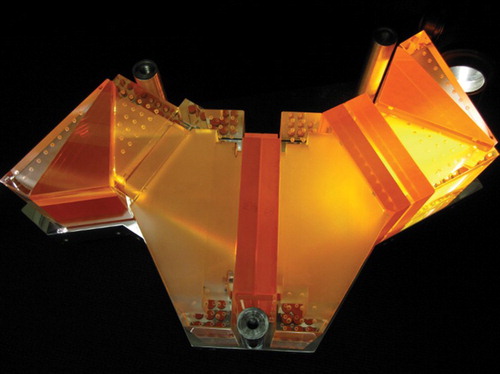
The SWIFT-DASH instrument is based on the original SWIFT instrument combined with a DASH interferometer. In this version, the solid Michelson interferometer is modified by replacing the mirrors with diffraction gratings; the monolithic optics for the developmental instrument are shown in Fig. 3, without the gratings attached. A plate beamsplitter is visible in the middle of the hexagon with the two arms on either side. Zinc selenide (ZnSe) is the infrared transmitting material; it appears reddish in visible light. The ZnSe elements are separated by spacers that are hollowed-out pieces of BSL7 glass, which has almost the same thermal expansion coefficient as ZnSe. In the current design, a 30° plate beamsplitter, field-widening prisms with an apex angle of 26.8°, a 45 mm thick compensating block of ZnSe, custom gratings with 189.474 lines per millimetre and hollow BSL7 spacers comprise the DASH optics.

Fig. 3 SWIFT-DASH monolithic optics assembly. The reddish elements are the ZnSe optical components. The clear BSL7 glass spacers are hollowed out in the optical path. The optics as shown are 540 mm wide, 260 mm deep, and 100 mm high.

To date, an interferometer design has been achieved that meets the requirements for the wind measurements identified in the SWIFT study. The ZnSe and BSL7 blocks composing the SHS/DMI were fabricated by LightMachinery, Ottawa. The current design gives a spectral resolution of 0.23 nm (0.029 cm⁻¹), which means that spectral lines of spacing greater than this can be resolved in the analysis. The theoretical maximum spectral range will be 31 nm (4 cm⁻¹).

The assembled instrument (approximately 540 mm × 260 mm × 100 mm), with gratings attached and in its holder, is shown in Fig. 4. The first fringes obtained from a pseudo-monochromatic spectral source are shown in Fig. 5. A tunable laser source at the required wavelengths was not available, so a pseudo-monochromatic spectral source was created using a narrow etalon (Full Width at Half Maximum (FWHM) 0.2 nm, Free Spectral Range (FSR) 4.8 nm), a medium etalon (FWHM 2.6 nm, FSR 60 nm), and a blocking filter (FWHM 180 nm centred at 8856.5 nm), with the temperature of the etalons tuned to overlap and lie within the spectral range of the SWIFT-DASH instrument. The filter combination results in one of the narrow etalon passbands transmitting radiation with adjacent passbands attenuated by the medium etalon that can be temperature tuned to select the transmitted wavelength. The fringes generated with this source have sufficient contrast to demonstrate that the observed fringes are real and repeatable. It should be noted that the finite width of the etalon passband results in a reduced contrast fringe compared with a monochromatic source such as a laser. The observations were taken with the SWIFT-DASH optics at room temperature and in air, whereas the optics were designed to work at 160 K and in a vacuum. The decrease in fringe contrast from the right-hand side to the left-hand side of Fig. 5 is consistent with operating at room temperature where the interferometer is not field widened. A high-temperature black-body source was used to fully fill the input field of view of the DASH optics. The etalon filter stack was placed in front of a commercial FLIR SC7300 L infrared camera at the exit of the DASH optics. The combination of no field widening at room temperature and the finite width of the etalon filter results in a reduced contrast fringe as observed. The next stage of the development work will be to cool the optics to an operating temperature of 160 K in a vacuum tank.

Fig. 4 SWIFT-DASH monolithic optics assembled in a rigid frame. The gratings are visible in each arm.

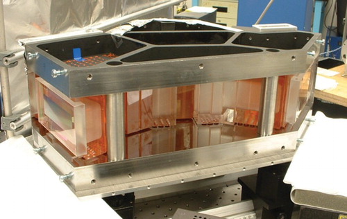
Fig. 5 Raw image of fringes observed following final assembly of the SWIFT-DASH monolithic optics. The observations were made at room temperature and in air with a FLIR SC7300 L IR camera (320 pixels × 256 pixels).

3 Retrieval of wind and ozone concentration

The optical thickness of the stratosphere due to ozone absorption is highly wavelength dependent because of the ro-vibrational nature of the absorption. In order to determine the most suitable line or lines to use for the retrieval of ozone number density, the dependence of the amplitude of the interferogram on tangent height was studied using a radiative transfer simulation (RTS) model (Rahnama et al., 2006) and a model of the DASH instrument developed by the authors. The ozone spectral region selected for the observations is shown in Fig. 6, about 1 cm⁻¹ width is displayed. The strongest eight lines in this spectral range are all due to the ν ₁ fundamental of ¹⁶O₃ (1103.14 cm⁻¹) (Barbe, Secroun, Jouve, Goldman, & Murcray, 1981). This spectral region will be isolated with an interference filter. Only a portion of the full instrument passband is simulated in order to reduce computational time for the simulations.

Fig. 6 Radiance spectra from the atmospheric radiative transfer model (RTS) developed for SWIFT. Spectra are simulated line by line at various tangent altitudes. Two isotopic N₂O lines and one NH₃ line are shown; these provide reference calibration lines.

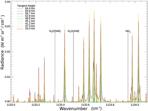
The nature of the problem is made clear with the ozone spectrum shown in Fig. 6. What is shown are calculated atmospheric spectra as observed from low Earth orbit for limb views through the atmosphere for the different tangent heights indicated. Simulations were performed for an infinitesimal field of view at each tangent height. Only one view direction was simulated, whereas the actual instrument will have two orthogonal views that can be combined to provide vector winds similar to the method used on WINDII. It can be seen that the lines broaden significantly at lower altitudes through pressure broadening, and it is this that determines the lowest altitudes at which winds can be measured.

One major advantage of the SHS/DMI approach is that the phase calibration line (providing a zero wind reference) and the atmospheric lines can be measured simultaneously across the entire field of the instrument and in every image because they appear as different Fourier components. This would be implemented by using a gas cell, containing either N₂O or NH₃, covering the entire field of view. The wavenumbers of two candidate calibration N₂O lines and one NH₃ line are shown. There is no need to remove the cell from the field of view so it can be permanently in place.

Although SHS is equivalent to FTS, SWIFT-DASH is not because it does not provide a complete interferogram, only a segment that does not include zero optical path difference. SWIFT-DASH therefore follows WINDII in analyzing the interferogram without converting it to a spectrum. A simulated amplitude spectrum for selected ozone lines is shown in Fig. 7. What is plotted are the amplitudes at the simulated fringe frequencies. The fringe frequency is defined to be, f = 4(σ − σ ₀)tan(θ_L ), where σ is the spectral wavenumber, σ ₀ is the Littrow wavenumber, and θ_L is the Littrow angle (Harlander et al., 1992). Amplitudes at integer fringe frequencies are derived using a harmonic analysis of the observed or simulated spatial interferogram. The actual spectrum of the ozone seen in Fig. 6 is not retrieved. Derived amplitudes are used in the wind and ozone number density retrievals.

Fig. 7 Altitude profiles of simulated amplitudes (given in Analogue to Digital Units (ADU) assuming a 14 bit Analogue to Digital Converter (ADC)) for selected fringe frequencies used in the retrievals.

a Ozone Concentration Retrieval

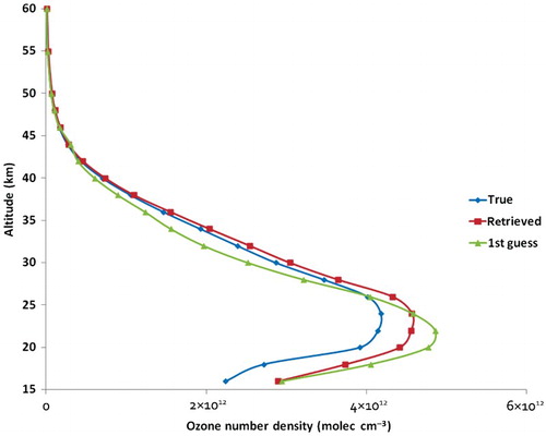
Not all fringe frequencies contain useful information, so one can select those that provide the most. For the ozone retrieval, because of absorption in the limb path, it turned out to be better to include fringe frequencies corresponding to the wings of the lines, that is for wavenumbers off the line centre used to define the fringe frequency. For the retrieval of the vertical distribution of ozone number density, the fringe frequency of choice is one for which the amplitude versus tangent height (hereafter named amplitude profile) appears to be correlated with the column of ozone along the line of sight (LOS). For fringe frequencies corresponding to the strongest ozone lines, the amplitude profile peaks at approximately 34 km for a 1976 US Standard Atmosphere, much higher than the ozone number density peak that, for the same atmosphere, peaks at 24 km. The column density along the LOS will tend to peak below the number density peak because of the cumulative (or integral) nature of the LOS column density. The frequencies chosen were 18, 31, and 32. Fringe frequency 31 is useful because it peaked slightly lower (23.452 versus 23.852 km) than fringe frequency 32 and 10 km lower than fringe frequency 18. The low radiance levels corresponding to these fringe frequencies are not problematic when 40 interferograms are averaged. The exposure time for each image is limited to 0.495 s by well depth and thermal background, so a set of 40 images requires 19.8 s elapsed time, which still provides good spatial coverage for a low Earth orbit limb instrument. Figure 8 shows the simulated “true” (mid-latitude summer) ozone profile, the “first guess profile” (1976 US Standard Atmosphere), and the “retrieved” profile. There is no a priori profile to influence the retrieved profile. The retrieval bias is dominated by a uniform −1 K bias in the temperature profile (forward model input). The retrieved profile agrees closely with the true profile down to 25 km, but there are differences below that. All sources of observational noise are incorporated including a realistic filter function. The Chahine method was used for this retrieval.

Fig. 8 Retrieved ozone (red) profile compared with a simulated mid-latitude summer “true” profile (blue). The first guess profile is shown in green.

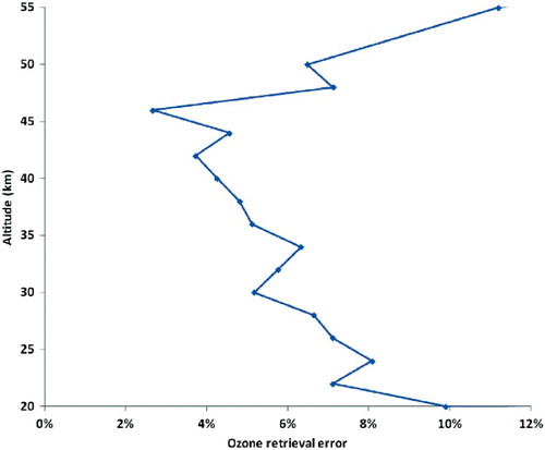
Figure 9 shows the ozone retrieval error as a percentage as a function of altitude. The ozone bias of 3 to 4% over 34 to 60 km is due to a −1 K bias in assumed temperature. The bias grows slightly and monotonically to 7% at 28 km and then increases dramatically below 20 km; thus, the forward model input error (temperature error) dominates the ozone error budget relative to observational noise sources. The temperature sensitivity arises mainly from errors in the Planck function not in the Boltzman distribution of the rotational lines. The positive bias is expected because larger ozone number densities compensate for the lower emitted radiance at an assumed lower temperature in the forward model. The discontinuity in shape is a result of random noise and convergence criteria applied to a single profile retrieval.

Fig. 9 Error in the retrieved ozone profile (percentage relative to “true”).

b Wind Retrieval

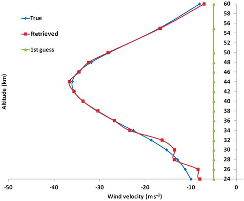
Figure 10 presents the results of the wind retrieval, showing the true profile (synthetic, with no geophysical significance), the first guess (the vertical line), and the retrieved wind. The retrieved wind is essentially indistinguishable from the true value from 60 km down to 34 km, whereas the error is evident but still very acceptable from 34 km down to 24 km. For this retrieval, the fringe frequencies of 10, 16, 19, and 28 were used. These correspond to lines with the following wavenumbers: 1133.43351, 1133.58691, 1133.6712, and 1133.97863 cm⁻¹. For the wind retrieval, the method described by Sioris, Kurosu, Martin, and Chance (2004) was employed.

Fig. 10 Retrieved wind profile (red) compared with simulated “true” (blue) profile. The first guess profile is shown in green.

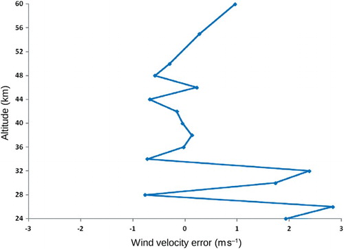
The wind error is shown as a function of altitude in Fig. 11. The wind error is less than 3 m s⁻¹ over the entire range of 24 to 60 km and significantly less above 34 km. The measurement of wind from phase clearly works well with this instrument. As with the ozone retrieval, a single wind profile was retrieved. This can be considered the a posteriori error although no a priori information was used to regularize the retrieval.

Fig. 11 Error in the retrieved wind profile (relative to “true”).

4 Conclusions

The capability of the combined DMI and SHS approach to measuring winds and ozone concentrations in the stratosphere has been demonstrated in two ways. The configuration called SWIFT-DASH has been designed, built, and operated in the laboratory, so far only for a monochromatic source. Simulated retrievals using these instrument characteristics have shown that the instrument can measure, from space, ozone concentrations to an accuracy of 10% over an altitude range of 20 to 55 km and winds to an accuracy of 3 m s⁻¹ from 24 to 60 km. Further tests using a laboratory ozone source are planned, and planning for a mission will follow. A Voigt line shape was used in the simulations and local thermal equilibrium (LTE) was assumed. There may be rotational and vibrational non-LTE effects that need to considered in future work.

Acknowledgements

The authors are grateful for the many individuals who supported the SWIFT, and later, SWIFT-DASH development. The Canadian Space Agency has been the primary supporter, but the Centre for Research in Earth and Space Technology (CRESTech) and the National Sciences and Engineering Research Council (NSERC) helped initiate the project. On the industrial side, we are particularly indebted to LightMachinery who fabricated this unique interferometer and COM DEV who prepared the basic design of the overall space instrument. Others from York University who contributed were Ian McDade, Bill Gault, Reza Mani, Peyman Rahnama, and Young-Min Cho. Special thanks go to Yves Rochon of Environment Canada for his continued expert contributions and advice.

References

- Barbe, A., Secroun, C., Jouve, P., Goldman, A., & Murcray, D. G. (1981). High-resolution infrared atmospheric spectra of ozone in the 10-μm region: Analysis of ν1 and ν3 bands- assignment of the (ν1 + ν2) - ν2 band. Journal of Molecular Spectroscopy, 86, 286–297. doi: 10.1016/0022-2852(81)90281-2
- Connes, P. (1958). Spectromètre interférential à selection par l'amplitude de modulation. Journal de Physique et le Radium, 19, 215–222. doi: 10.1051/jphysrad:01958001903021500
- Englert, C. R., Babcock, D. D., & Harlander, J. M. (2007). Doppler Asymmetric Spatial Heterodyne spectroscopy (DASH): concept and experimental demonstration. Applied Optics, 46, 7297–7307. doi: 10.1364/AO.46.007297
- Harlander, J., Reynolds, R. J., & Roesler, F. L. (1992). Spatial heterodyne spectroscopy for the exploration of diffuse interstellar emission lines at far-ultraviolet wavelengths. The Astrophysical Journal, 396, 730–740. doi: 10.1086/171756
- Hilliard, R. L., & Shepherd, G. G. (1966). Wide-angle Michelson interferometer for measuring Doppler line widths. Journal of the Optical Society of America, 56, 362–369. doi: 10.1364/JOSA.56.000362
- Rahnama, P., Rochon, Y. J., McDade, I. C., Shepherd, G. G., Gault, W. A., & Scott, A. (2006). Satellite measurements of stratospheric winds and ozone using Doppler Michelson interferometry. Part I: Instrument model and measurement simulation. Journal of Atmospheric and Oceanic Technology, 23, 753–769. doi: 10.1175/JTECH1880.1
- Shepherd, G. G. (2002). Spectral imaging of the atmosphere. Amsterdam: Academic Press.
- Shepherd, G. G., Gault, W. A., Miller, D. W., Pasturczyk, Z., Johnston, S. F., Kosteniuk, P. R., … Wimperis, J. R. (1985). WAMDII: Wide Angle Michelson Doppler Imaging Interferometer for Spacelab. Applied Optics, 24, 1571–1584. doi: 10.1364/AO.24.001571
- Shepherd, G. G., McDade, I. C., Gault, W. A., Rochon, Y. J., Scott, A., Rowlands, N., & Buttner, G. (2001). The Stratospheric Wind Interferometer for Transport studies (SWIFT). Advances in Space Research, 27, 1071–1079. doi: 10.1016/S0273-1177(01)00140-5
- Shepherd, G. G., Thuillier, G., Cho, Y.-M., Duboin, M.-L., Evans, W. F. J., Gault, W. A., … Ward, W. E. (2012). The Wind Imaging Interferometer (WINDII) on the Upper Atmosphere Research Satellite: A twenty-year perspective. Reviews of Geophysics, 50, RG2007. doi:10.1029/2012RG000390
- Shepherd, G. G., Thuillier, G., Gault, W. A., Solheim, B. H., Hersom, C., Alunni, J. M., … Wimperis, J. (1993). WINDII, the wind imaging interferometer on the Upper Atmosphere Research Satellite. Journal of Geophysical Research, 98, 10725–10750. doi: 10.1029/93JD00227
- Sioris, C. E., Kurosu, T. P., Martin, R. V., & Chance, K. (2004). Stratospheric and tropospheric NO2 observed by SCIAMACHY: First results. Advances in Space Research, 34, 780–785. doi: 10.1016/j.asr.2003.08.066
- Zhang, S. P., McLandress, C., & Shepherd, G. G. (2007). Satellite observations of mean winds and tides in the lower thermosphere. Part 2: WINDII monthly winds for 1992 and 1993. Journal of Geophysical Research, 112(D21), D21105. doi:10.1029/2007JD008457