Trends and Variability in Total Ozone from a Mid-Latitude Southern Hemisphere Site: The Melbourne Dobson Record 1978–2012

Abstract

The Australian Bureau of Meteorology maintains a number of long-running Dobson measurement programs, among the few in southern hemisphere mid-latitudes. Data from the Melbourne site (the Melbourne/Airport World Ozone and Ultraviolet Radiation Data Centre (WOUDC) station was originally located at Aspendale, then moved to the city centre, and finally to Melbourne Airport) from 1978 to 2012 have recently been reviewed and re-evaluated. These data are analyzed using multi-linear regression and also by application of an 11-year running mean. Satellite data from the Merged Ozone Dataset are also used for comparison with the Dobson results. We show that the Quasi-Biennial Oscillation (QBO) plays a major role in winter and spring once phase is taken into account by month. We also show that the three so-called “classical” proxies (QBO, solar cycle, and Equivalent Effective Stratospheric Chlorine (EESC)) alone are able to give a good fit to ozone for Melbourne and, more generally, the southern mid-latitudes for most months of the year, in contrast with the case in the northern hemisphere where dynamical variation plays a much more important role. Correspondingly, the smoothed Melbourne Dobson time series shows a high correlation to EESC.

Résumé

[Traduit par la rédaction] Le Bureau of Meteorology d'Australie maintient un certain nombre de programmes de mesures Dobson de longue haleine, un des rares programmes pour les latitudes moyennes de l'hémisphère Sud. Les données du site de Melbourne (la station du Melbourne/Airport World Ozone and Ultraviolet Radiation Data Centre (WOUDC) était initialement située à Aspendale, puis a été déménagée au centre de la ville et finalement à l'aéroport de Melbourne) de 1978 à 2012 ont récemment été passées en revue et réévaluées. Nous analysons ces données au moyen de la régression linéaire multiple et aussi par l'application d'une moyenne mobile de 11 ans. Nous utilisons aussi les données satellitaires du Merged Ozone Dataset pour la comparaison avec les résultats Dobson. Nous montrons que l'oscillation quasi-biennale joue un rôle majeur en hiver et au printemps lorsque la phase est prise en considération pour chaque mois. Nous montrons aussi que les trois variables explicatives dites « classiques » (oscillation quasi-biennale, cycle solaire et équivalent chlore stratosphérique efficace) peuvent à elles seules produire une bonne repr/sentation de l'ozone à Melbourne et, plus généralement, aux latitudes moyennes Sud pour la plupart des mois de l'année, contrairement au cas de l'hémisphère Nord où les variations dynamiques jouent un rôle beaucoup plus important. De ce fait, la série chronologique lissée des données Dobson de Melbourne affiche une corrélation élevée avec l’équivalent chlore stratosphérique efficace.

Keywords:

• chemistry
• intraseasonal variability
• mid-latitudes
• stratosphere
• southern hemisphere
• observation
• ozone
• Dobson

1 Introduction

The Australian Bureau of Meteorology currently operates four Dobson spectrophotometer (Dobson, 1931) sites (Table 1), as well as a fifth location, Perth, in conjunction with the United States National Oceanic and Atmospheric Administration (NOAA). Although Dobson measurements at all sites have long and important records, much of the old data are currently in need of review to ensure a traceable history and consistency of processing. Such a review process has recently been undertaken for the Melbourne site for 1978 to 2012. For operational reasons, the actual measurement location has moved slightly over this period resulting in different names and station numbers at the World Meteorological Organization (WMO) World Ozone and Ultraviolet Radiation Data Centre (WOUDC); Melbourne/Airport (STN 253) includes measurements from both the Aspendale (STN 26) and city centre locations. However, we have not been able to detect any evidence of shifts or inhomogeneities in the data as a result of the moves and, therefore, consider the dataset to be a single record.

Table 1. The Dobson spectrophotometer sites in the Australian Bureau of Meteorology network. The WOUDC station number is given in parentheses after the station name.

Name (Station Number)	Latitude	Years of Operation
Darwin (STN 84)	12°S	1966–74, 1992–present
Brisbane (STN 27)	27°S	1957–present
Aspendale (STN 26), Melbourne/Airport (STN 253)	38°S	1957–present
Macquarie Island (STN 29)	55°S	1957–present

The resulting dataset has been analyzed in two ways, using the standard method of multi-linear regression (MLR) against selected proxy time series, and also, following Angell and Free (2009), by applying an 11-year running mean to remove the influence of proxies with near-constant periodicity (the annual cycle, Quasi-Biennial Oscillation (QBO), and 11-year solar cycle). Some comparisons are also made by performing the same analysis using data from the Merged Ozone Dataset (MOD; which uses data from the satellite-based Total Ozone Mapping Spectrometer/Ozone Monitoring Instrument (TOMS/OMI) and the Solar Backscatter Ultraviolet (SBUV) series instruments), concentrating on southern hemisphere (SH) mid-latitudes.

aDescription of Data

All network Dobson instruments used in Melbourne from 1978 to 2012 are traceable to the Regional Standard (Dobson 105) and from there to the World Standard, with documented intercomparisons. The ozone values have been recalculated using a consistent algorithm for all terms. (Bass and Paur cross-sections (Komhyr, Mateer, & Hudson, 1993) have been used following the still current recommendation.) Monthly-mean values of the full record are shown in Fig. 1. These have been calculated using Direct Sun (“DS”) and AD-wavelength pairs only, avoiding the extra uncertainty associated with zenith corrections. The time series has been deseasonalized by subtracting the monthly mean, calculated over the full period, from each value.

Fig. 1 Melbourne Dobson monthly mean total ozone, deseasonalized by subtracting the 1978–2012 monthly mean from each value.

The MOD (Stolarski & Frith, 2006) combines data from the TOMS/OMI and SBUV series of instruments onboard a long sequence of satellite platforms to give a near continuous dataset over the period covered by the reprocessed Dobson data. Here we will make use of both zonally averaged data and also data gridded into 10° × 5° bins (NASA, 2012a). Figure 2 shows a scatterplot of the Dobson monthly means against the values from the MOD grid cell corresponding to the location of Melbourne, centred on 145°E 37.5°S. Over this range of values there is a near-constant offset of about 3 Dobson Units (DU; 1 DU = 0.01 mm at standard temperature and pressure and is equivalent to 2.69 × 10²⁰ molecules per square metre), with the MOD values being higher than the Dobson values.

Fig. 2 Comparison of Melbourne Dobson monthly mean values with MOD values from the corresponding grid cell. The dashed line indicates the linear fit.

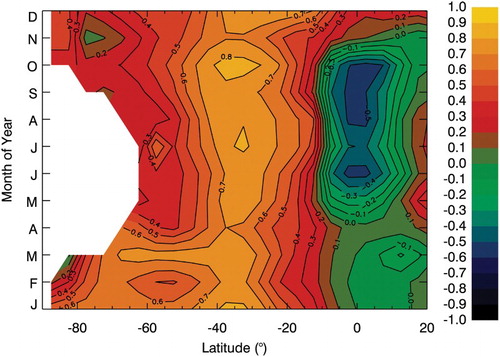
One point of interest is the extent to which a single available measurement site is representative of large-scale patterns. Using MOD data, Fig. 3 shows the correlation of monthly mean ozone in the grid cell corresponding to the location of Melbourne (centred on 145°E 37.5°S), with the zonal mean ozone value by latitude and month. Ozone variation at this location is well correlated with the zonal mean for all months of the year (correlation coefficient R > 0.7) except November, and further, with much of the SH mid-latitudes, particularly in January and February when the entire SH extratropical region is well correlated, as noted by Fioletov and Shepherd (2003, 2005), Tegtmeier and Shepherd (2007), and Tegtmeier, Fioletov, and Shepherd (2008). Also evident is a clear anticorrelation in winter and spring with the tropics north of 12.5°S.

Fig. 3 Correlation between zonal mean ozone values for each month and the grid cell representing the location of the Melbourne Dobson (centred on 145°E 37.5°S), using MOD data.

2 Smoothing

The technique of applying an 11-year running mean to smooth ozone time series was used by Angell and Free (2009) to remove the effects of well-established influences on ozone that have a regular periodicity, namely the annual cycle, the QBO, and the 11-year solar cycle. This very simple procedure overcomes certain potential disadvantages of MLR such as the proxy being used may not fully represent the actual physical process. However, it cannot yield the same level of insight into physical processes. Self-evidently, smoothing will also remove the effect of unbiased scatter but not that of non-periodic terms such as changes in stratospheric aerosol loading or dynamical trends.

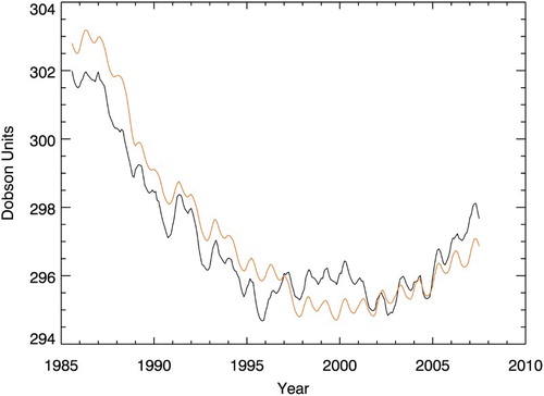
Figure 4 shows the result of applying the 11-year running mean to the Melbourne Dobson spectrophotometer data, with the first five years and last five years omitted. A strong correlation with Equivalent Effective Stratospheric Chlorine (EESC), calculated with an age of air of four years, is evident (correlation coefficient R = 0.97). (The EESC values used here were obtained from the Goddard auto-mailer service (Newman, Daniel, Waugh, & Nash, 2007).) Using this technique gives a fit of smoothed ozone to EESC of 0.0090 ± 0.0001 DU/ppt.

Fig. 4 Melbourne Dobson monthly means smoothed by an 11-year running mean (black diamonds) and corresponding MOD values representing the same location also smoothed by 11 years (blue diamonds), both with a fit to EESC (green curves).

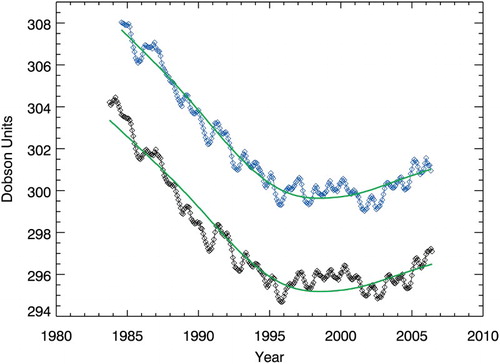
The corresponding MOD data (again using the gridded data for the same location as Melbourne) are also shown. Although the offset of approximately 3 DU seen in Fig. 2 between the satellite- and ground-based time series is very evident, both the high and low frequency variations correspond very well. A similar correlation with EESC is also found (R = 0.98), and the linear fit term is 0.0095 ± 0.0001 DU/ppt.

In fact, throughout the SH mid-latitudes from 30°–60°S, smoothed zonal mean ozone is similarly well correlated with four-year EESC (R > 0.98); however, this is not the case in the northern hemisphere (NH).

3 Multi-linear regression

Numerous recent studies have made use of MLR of ozone time series against a set of fairly standard proxies that have been found to usefully represent physical processes that influence ozone (Bodeker, Garny, Smale, Dameris, & Deckert, 2007; Brunner, Staehelin, Maeder, Wohltmann, & Bodeker, 2006; Dhomse, Weber, Wohltmann, Rex, & Burrows, 2006; Fischer et al., 2008; Fleming, Jackman, Weisenstein, & Ko, 2007; Harris et al., 2008; Jones et al., 2009; Kiesewetter, Sinnhuber, Weber, & Burrows, 2010; Krzys´cin, 2010; Mäder et al., 2007, 2010; Manzini et al., 2010; Randel & Wu, 2007; Reinsel et al., 2005; Steinbrecht, Hassler, Claude, Winkler, & Stolarski, 2003; Steinbrecht et al., 2006, 2011; Wohltmann, Lehmann, Rex, Brunner, & Mäder, 2007; Wohltmann, Rex, Brunner, & Mäder, 2005). An alternative method (Principal Component Analysis) was used to study the SH extratropics in Jiang et al. (2008), while extreme high or low ozone events were studied in addition to means in Frossard et al. (2013) and Rieder et al. (2013).

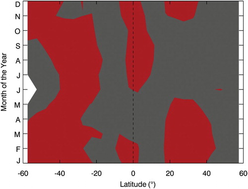
In our MLR analysis of the Dobson time series we restrict ourselves to only the three proxies Brunner et al. (2006) considered the “classical proxies,” EESC, QBO, and the 11-year solar cycle, and do not take into account either variations in stratospheric aerosol or the commonly used dynamic proxies such as the Eliassen-Palm Flux or the Antarctic Oscillation. This approach is motivated by Fig. 5 which shows that the classical proxies alone are able to account for a significant fraction of the variation in ozone in SH mid-latitudes for the entire year, unlike in the NH. (The values of the proxies were obtained from the Goddard auto-mailer as above for EESC, from NOAA (2012) “50 mb zonal wind index” to represent the QBO, and from NASA (2012b) for the solar cycle.)

Fig. 5 Region where the total correlation between the MOD zonal mean ozone values and the three “classical” proxies (with EESC age-of-air set to three years) have correlation coefficients R > 0.8 (red) or R < 0.8 (grey) by month and latitude. The SH mid-latitudes from 30°–60°S are well described apart from winter poleward of about 50°S, in contrast to the NH.

In accounting for this difference between the hemispheres, there are several points of distinction to be considered:

1. The Brewer Dobson circulation is weaker in the SH, and there is less variability because of the dynamics at mid-latitudes (for the corresponding latitude) (Staehelin, Harris, Appenzeller, & Eberhard, 2001).

2. The extent of polar ozone depletion from year to year is much more consistent in the Antarctic than in the Arctic (Brunner et al., 2006).

3. The ozone distribution is more zonally symmetric in the SH, with a regular feature of a pronounced wave-1 pattern developing in spring around 65°S (Gabriel et al., 2011; Hitchman & Rogal, 2010; Ialongo, Sofieva, Kalakoski, Tamminen, & Kyrölä, 2012; Kravchenko et al., 2012; Lozitsky, Grytsai, Klekociuk, & Milinevsky, 2011).

4. The impact of the Mount Pinatubo eruption is harder to find in the SH (Aquila, Oman, Stolarski, Colarco, & Newman, 2012; Aquila, Oman, Stolarski, Douglass, & Newman, 2012; Poberaj, Staehelin, & Brunner, 2011; Telford, Braesicke, Morgenstern, & Pyle, 2009).

a Quasi-Biennial Oscillation

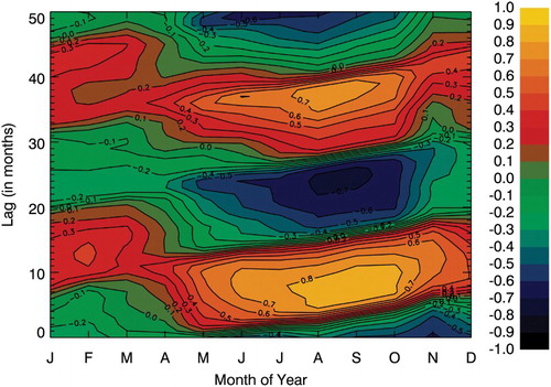
The dominant variability from year to year apparent in the Melbourne Dobson data is the effect of the QBO in winter and spring as shown in Fig. 6. In fact the strong influence of the QBO on Australian data was noted many years ago (Kulkarni, 1980). The phase relationship for maximum correlation is not constant but varies in a continuous but regular manner from month to month. The same correlation pattern also emerges clearly in MOD zonal mean data for the corresponding latitude band (Fig. 7). Although a similar pattern (displaced by six months) can be seen for the corresponding latitude in the NH, in general the phase of maximum correlation is latitude dependent.

Fig. 6 Correlation between Melbourne Dobson mean ozone (detrended) and the QBO at 50 hPa by month and lag.

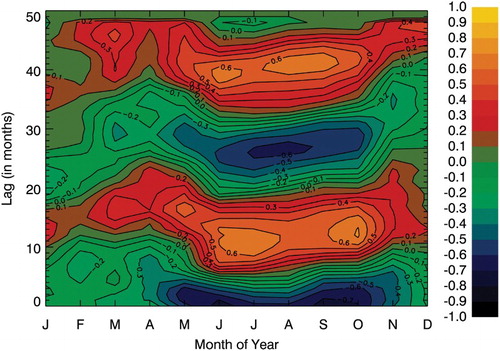
Fig. 7 Correlation between MOD 35°–40°S zonal mean ozone (detrended) and QBO at 50 hPa by month and lag.

Although the existence of an ozone QBO effect extending poleward of the equatorial region has been recognized for many years (Baldwin et al., 2001 and references therein), the magnitude is often underestimated and the phase relationship is only sometimes considered in sufficient detail (Anstey & Shepherd, 2008; Echer, Guarnieri, Rigozo, & Vieira, 2004; Hampson & Haynes, 2006; Punge & Giorgetta, 2008; Randel & Wu, 1996; Schoeberl et al., 2008; Sitnov, 2006; Yang & Tung, 1995). The phase pattern throughout the year was partly identified in Bowman (1989) and is evidently a result of the interaction of the QBO with the annual cycle of the Brewer Dobson circulation (Ziemke & Chandra, 2012). We find the peak-to-peak size of the QBO effect in total ozone in winter in both hemispheres averaged between 15° and 50° is almost 20 DU.

Although the importance of variation in planetary wave driving affecting interannual ozone variability has often been emphasized in the literature (Dhomse et al., 2006; Fusco & Salby, 1999; Gabriel & Schmitz, 2003; Hood & Soukharev, 2005; Huck, McDonald, Bodeker, & Struthers, 2005; Miyazaki, Iwasaki, Shibata, & Deushi, 2005; Monier & Weare, 2011; Nathan, Cordero, Li, & Wuebbles, 2000; Randel, Wu, & Stolarski, 2002; Salby, 2011; Salby & Callaghan, 2002; Salby, Titova, & Deschamps, 2011; Weber et al., 2003, 2011), we find, that for SH mid-latitudes it does not play a very significant role until poleward of at least 50°S.

4 Regression to Melbourne Dobson data

Motivated by Fig. 5 we apply MLR analysis to the Melbourne Dobson record, making use of only the three proxies. It is found that, to obtain the best correlation, an older age of air should be applied for the summer months (six years), decreasing progressively in age until spring (three years). Although not further investigated here, this is consistent with the notion of older air from the polar vortex mixing into the general circulation after the vortex breaks down (Stiller et al., 2012).

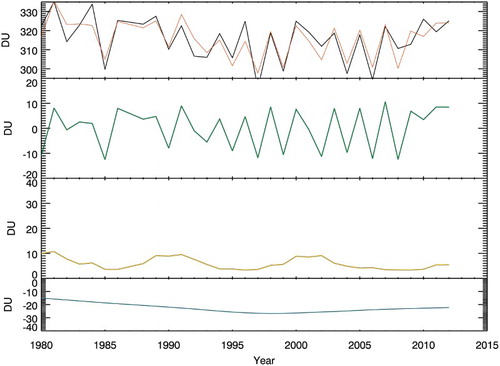
Figures 8 and 9 show the relative contributions made by the three proxies for the three summer months (December, January, and February) and the three winter months (June, July, and August). The QBO dominates in winter while the contributions from EESC and the solar cycle are more consistent over the entire year. The year-to-year variability is captured much better in winter, but the contribution of the solar cycle plus EESC to the underlying trend in summer is clear.

Fig. 8 Melbourne Dobson summer (December, January, and February) mean values (top, black) and MLR fit (orange). The contributions to the fit of, respectively, the QBO, the solar cycle, and EESC are shown in green (second from top), yellow (third from top). and blue (bottom).

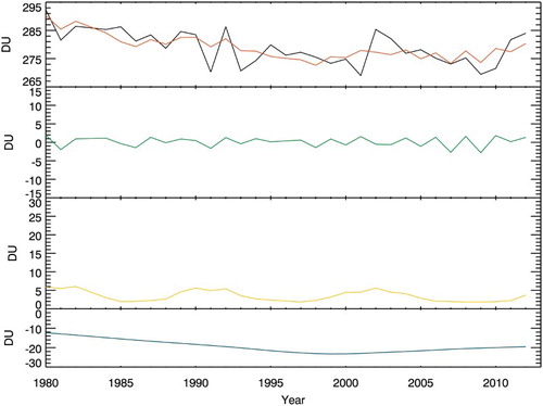
Fig. 9 Melbourne Dobson winter (June, July, and August) mean values (top, black) and MLR fit (orange). The contributions to the fit of, respectively, the QBO, the solar cycle, and EESC are shown in green (second from top), yellow (third from top), and blue (bottom).

Figure 10 shows the total fit against the observed time series. In general, the fit performs very well but does not fully capture a significant number of the yearly maxima and minima. The residuals are shown in Fig. 11. In contrast to Fig. 1 there are now no significant trends and much of the variability has been accounted for, although there still remain particular short episodes of anomalously high or low ozone which would warrant further individual investigation.

Fig. 10 Fitted time series (orange) compared with observational data (black).

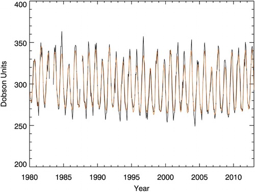
Fig. 11 Residuals obtained by subtracting the fitted time series from the observed data.

Finally, for comparison with Fig. 4, the same smoothing (11 years) is also applied to the MLR fitted time series in Fig. 12. This illustrates the consistency of the two approaches taken. Because two of the three proxies used to obtain the fit are periodic, the fit will therefore tend closer and closer to EESC after smoothing. Similar to Fig. 4, the fit in Fig. 12 is again slightly low (less than 1 DU) in the period between 1998 and 2001. The correlation coefficient between the two smoothed time series is R = 0.97.

Fig. 12 Observed Dobson data smoothed by an 11-year running mean (black), and the fit obtained from MLR also smoothed by the same amount (orange).

5 Conclusions

Using consistently reprocessed ozone data from the long-running Melbourne Dobson site, two different methods of analysis—MLR and simple smoothing—have been used to suggest that ozone in the SH mid-latitudes is following a trend very consistent with that expected from the rise and decline of EESC. It is argued that a very simple set of proxies is more adequately able to account for the variation in the ozone time series in the SH than in the NH, in particular noting the large role of QBO variability in winter and spring. The results from the Dobson record are in good agreement with satellite data from the Merged Ozone Dataset.

Interestingly, Weatherhead et al. (2000), Reinsel et al. (2002) and more recently Vyushin, Fioletov, and Shepherd (2007), Vyushin, Shepherd, and Fioletov (2010) have nominated the SH mid-latitudes as one of the first areas in the world where ozone recovery is predicted to be statistically detectable.

Acknowledgements

Part of this work was performed under Projects 737 and 4012 of the Australian Antarctic Science programme. The authors would like to thank NASA Goddard Space Flight Center for producing and making available the Merged Ozone Dataset as well as all the many observers from both the Bureau of Meteorology and the Commonwealth Scientific and Industrial Research Organization (CSIRO) who made Dobson observations from 1978 to 2012.

References

- Angell, J. K., & Free, M. (2009). Ground-based observations of the slowdown in ozone decline and onset of ozone increase. Journal of Geophysical Research, 114(D7). doi:10.1029/2008JD010860
- Anstey, J. A., & Shepherd, T. G. (2008). Response of the northern stratospheric polar vortex to the seasonal alignment of QBO phase transitions. Geophysical Research Letters, 35(22). doi:10.1029/2008GL035721
- Aquila, V., Oman, L. D., Stolarski, R., Douglass, A. R., & Newman, P. A. (2012). The response of ozone and nitrogen dioxide to the eruption of Mt. Pinatubo at southern and northern midlatitudes. Journal of the Atmospheric Sciences, 70, 894–900. doi:10.1175/JAS-D-12-0143.1
- Aquila, V., Oman, L. D., Stolarski, R. S., Colarco, P. R., & Newman, P. A. (2012). Dispersion of the volcanic sulfate cloud from a Mount Pinatubo–like eruption. Journal of Geophysical Research, 117(D6). doi:10.1029/2011JD016968
- Baldwin, M. P., Gray, L. J., Dunkerton, T. J., Hamilton, K., Haynes, P. H., Randel, W. J., & Takahashi, M. (2001). The quasi-biennial oscillation. Reviews of Geophysics, 39(2), 179. doi:10.1029/1999RG000073
- Bodeker, G. E., Garny, H., Smale, D., Dameris, M., & Deckert, R. (2007). The 1985 southern hemisphere mid-latitude total column ozone anomaly. Atmospheric Chemistry and Physics, 7(21), 5625–5637. doi:10.5194/acp-7-5625-2007
- Bowman, K. P. (1989). Global patterns of the quasi-biennial oscillation in total ozone. Journal of the Atmospheric Sciences, 46(21), 3328–3343. doi:10.1175/1520-0469(1989)046<3328:GPOTQB>2.0.CO;2
- Brunner, D., Staehelin, J., Maeder, J. A., Wohltmann, I., & Bodeker, G. E. (2006). Variability and trends in total and vertically resolved stratospheric ozone based on the CATO ozone data set. Atmospheric Chemistry and Physics, 6(12), 4985–5008. doi:10.5194/acp-6-4985-2006
- Dhomse, S., Weber, M., Wohltmann, I., Rex, M., & Burrows, J. P. (2006). On the possible causes of recent increases in northern hemispheric total ozone from a statistical analysis of satellite data from 1979 to 2003. Atmospheric Chemistry and Physics, 6(5), 1165–1180. doi:10.5194/acp-6-1165-2006
- Dobson, G. M. B. (1931). A photoelectric spectrophotometer for measuring the amount of atmospheric ozone. Proceedings of the Physical Society, 43, 324. doi:10.1088/0959-5309/43/3/308
- Echer, E., Guarnieri, F. L., Rigozo, N. R., & Vieira, L. E. A. (2004). A study of the latitudinal dependence of the quasi-biennial oscillation in Total Ozone Mapping Spectrometer total ozone. Tellus A, 56(5), 527–535. doi:10.1111/j.1600-0870.2004.00080.x
- Fioletov, V. E., & Shepherd, T. G. (2003). Seasonal persistence of midlatitude total ozone anomalies. Geophysical Research Letters, 30(7). doi:10.1029/2002GL016739
- Fioletov, V. E., & Shepherd, T. G. (2005). Summertime total ozone variations over middle and polar latitudes. Geophysical Research Letters, 32(4). doi:10.1029/2004GL022080
- Fischer, A. M., Schraner, M., Rozanov, E., Kenzelmann, P., Schnadt Poberaj, C., Brunner, D., & Brönnimann, S. (2008). Interannual-to-decadal variability of the stratosphere during the 20th century: Ensemble simulations with a chemistry-climate model. Atmospheric Chemistry and Physics, 8(24), 7755–7777. doi:10.5194/acp-8-7755-2008
- Fleming, E. L., Jackman, C. H., Weisenstein, D. K., & Ko, M. K. W. (2007). The impact of interannual variability on multidecadal total ozone simulations. Journal of Geophysical Research, 112(D10). doi:10.1029/2006JD007953
- Frossard, L., Rieder, H. E., Ribatet, M., Staehelin, J., Maeder, J. A., Di Rocco, S., & Peter, T. (2013). On the relationship between total ozone and atmospheric dynamics and chemistry at mid-latitudes – Part 1: Statistical models and spatial fingerprints of atmospheric dynamics and chemistry. Atmospheric Chemistry and Physics, 13(1), 147–164. doi:10.5194/acp-13-147-2013
- Fusco, A. C., & Salby, M. L. (1999). Interannual variations of total ozone and their relationship to variations of planetary wave activity. Journal of Climate, 12(6), 1619–1629. doi:10.1175/1520-0442(1999)012<1619:IVOTOA>2.0.CO;2
- Gabriel, A., Körnich, H., Lossow, S., Peters, D. H. W., Urban, J., & Murtagh, D. (2011). Zonal asymmetries in middle atmospheric ozone and water vapour derived from Odin satellite data 2001–2010. Atmospheric Chemistry and Physics, 11(18), 9865–9885. doi:10.5194/acp-11-9865-2011
- Gabriel, A., & Schmitz, G. (2003). The influence of large-scale eddy flux variability on the zonal mean ozone distribution. Journal of Climate, 16(15), 2615–2627. doi:10.1175/1520-0442(2003)016<2615:TIOLEF>2.0.CO;2
- Hampson, J., & Haynes, P. (2006). Influence of the equatorial QBO on the extratropical stratosphere. Journal of the Atmospheric Sciences, 63(3), 936–951. doi:10.1175/JAS3657.1
- Harris, N. R. P., Kyrö, E., Staehelin, J., Brunner, D., Andersen, S.-B., Godin-Beekmann, S., & Zerefos, C. (2008). Ozone trends at northern mid- and high latitudes – a European perspective. Annales Geophysicae, 26(5), 1207–1220. doi:10.5194/angeo-26-1207-2008
- Hitchman, M. H., & Rogal, M. J. (2010). Influence of tropical convection on the southern hemisphere ozone maximum during the winter to spring transition. Journal of Geophysical Research, 115(D14). doi:10.1029/2009JD012883
- Hood, L. L., & Soukharev, B. E. (2005). Interannual variations of total ozone at northern midlatitudes correlated with stratospheric EP flux and potential vorticity. Journal of the Atmospheric Sciences, 62(10), 3724–3740. doi:10.1175/JAS3559.1
- Huck, P. E., McDonald, A. J., Bodeker, G. E., & Struthers, H. (2005). Interannual variability in Antarctic ozone depletion controlled by planetary waves and polar temperature. Geophysical Research Letters, 32(13). doi:10.1029/2005GL022943
- Ialongo, I., Sofieva, V., Kalakoski, N., Tamminen, J., & Kyrölä, E. (2012). Ozone zonal asymmetry and planetary wave characterization during Antarctic spring. Atmospheric Chemistry and Physics, 12(5), 2603–2614. doi:10.5194/acp-12-2603-2012
- Jiang, X., Pawson, S., Camp, C. D., Nielsen, J. E., Shia, R.-L., Liao, T., & Yung, Y. L. (2008). Interannual variability and trends of extratropical ozone. Part II: Southern hemisphere. Journal of the Atmospheric Sciences, 65(10), 3030–3041. doi:10.1175/2008JAS2793.1
- Jones, A., Urban, J., Murtagh, D. P., Eriksson, P., Brohede, S., Haley, C., & Burrows, J. (2009). Evolution of stratospheric ozone and water vapour time series studied with satellite measurements. Atmospheric Chemistry and Physics, 9(16), 6055–6075. doi:10.5194/acp-9-6055-2009
- Kiesewetter, G., Sinnhuber, B.-M., Weber, M., & Burrows, J. P. (2010). Attribution of stratospheric ozone trends to chemistry and transport: A modelling study. Atmospheric Chemistry and Physics, 10(24), 12073–12089. doi:10.5194/acp-10-12073-2010
- Komhyr, W. D., Mateer, C. L., & Hudson, R. D. (1993). Effective Bass-Paur 1985 ozone absorption coefficients for use with Dobson ozone spectrophotometers. Journal of Geophysical Research, 98(D11), 20451. doi:10.1029/93JD00602
- Kravchenko, V. O., Evtushevsky, O. M., Grytsai, A. V., Klekociuk, A. R., Milinevsky, G. P., & Grytsai, Z. I. (2012). Quasi-stationary planetary waves in late winter Antarctic stratosphere temperature as a possible indicator of spring total ozone. Atmospheric Chemistry and Physics, 12(6), 2865–2879. doi:10.5194/acp-12-2865-2012
- Krzys´cin, J. W. (2010). Onset of the total ozone increase based on statistical analyses of global ground-based data for the period 1964–2008. International Journal of Climatology, 32(2), 240–246. doi:10.1002/joc.2264
- Kulkarni, R. N. (1980). Atmospheric ozone over Australia – A review. Pure and Applied Geophysics, 118(1), 387–400. doi:10.1007/BF01586460
- Lozitsky, V., Grytsai, A., Klekociuk, A., & Milinevsky, G. (2011). Influence of planetary waves on total ozone column distribution in northern and southern high latitudes. International Journal of Remote Sensing, 32(11), 3179–3186. doi:10.1080/01431161.2010.541519
- Mäder, J. A., Staehelin, J., Brunner, D., Stahel, W. A., Wohltmann, I., & Peter, T. (2007). Statistical modeling of total ozone: Selection of appropriate explanatory variables. Journal of Geophysical Research, 112(D11). doi:10.1029/2006JD007694
- Mäder, J. A., Staehelin, J., Peter, T., Brunner, D., Rieder, H. E., & Stahel, W. A. (2010). Evidence for the effectiveness of the Montreal Protocol to protect the ozone layer. Atmospheric Chemistry and Physics, 10(24), 12161–12171. doi:10.5194/acp-10-12161-2010
- Manzini, E., and Matthes, K. (Lead Authors) Blume, C., Bodeker, G., Cagnazzo, C., Calvo, N., … Yoden, S., (2010) Natural variability of stratospheric ozone. In V. Eyring, T. G. Shepherd, & D. W. Waugh (Eds.) Report on the Evaluation of Chemistry-Climate Models (Chapter 8) WCRP-132, WMO/TD-No. 1526. Retrieved from http://www.sparc-climate.org/publications/sparc-reports/sparc-report-no5/
- Miyazaki, K., Iwasaki, T., Shibata, K. & Deushi, M. (2005). Roles of transport in the seasonal variation of the total ozone amount. Journal of Geophysical Research, 110(D18). doi:10.1029/2005JD005900
- Monier, E., & Weare, B. C. (2011). Climatology and trends in the forcing of the stratospheric ozone transport. Atmospheric Chemistry and Physics, 11(13), 6311–6323. doi:10.5194/acp-11-6311-2011
- NASA (National Aeronautics and Space Administration). (2012a). Merged ozone dataset [Data]. Goddard Space Flight Center, Atmospheric Chemistry and Dynamics Laboratory. Retrieved from http://acdb-ext.gsfc.nasa.gov/Data_services/
- NASA (National Aeronautics and Space Administration). (2012b). Observed monthly solar flux [Data]. Goddard Space Flight Center, Solar Data Analysis Centre. Retrieved from http://umbra.nascom.nasa.gov/index.html/
- Nathan, T. R., Cordero, E. C., Li, L., & Wuebbles, D. J. (2000). Effects of planetary wave-breaking on the seasonal variation of total column ozone. Geophysical Research Letters, 27(13), 1907. doi:10.1029/1999GL010891
- Newman, P. A., Daniel, J. S., Waugh, D. W., & Nash, E. R. (2007). A new formulation of equivalent effective stratospheric chlorine (EESC). Atmospheric Chemistry and Physics, 7(17), 4537–4552. doi:10.5194/acp-7-4537-2007
- NOAA (National Oceanic and Atmospheric Administration). (2012). Monthly atmospheric and SST indices [Data]. National Weather Service, Climate Prediction Center. Retrieved from http://www.cpc.noaa.gov/data/indices/
- Poberaj, C. S., Staehelin, J., & Brunner, D. (2011). Missing stratospheric ozone decrease at southern hemisphere middle latitudes after Mt. Pinatubo: A dynamical perspective. Journal of the Atmospheric Sciences, 68(9), 1922–1945. doi:10.1175/JAS-D-10-05004.1
- Punge, H. J., & Giorgetta, M. A. (2008). Net effect of the QBO in a chemistry climate model. Atmospheric Chemistry and Physics, 8(21), 6505–6525. doi:10.5194/acp-8-6505-2008
- Randel, W. J., & Wu, F. (1996). Isolation of the ozone QBO in SAGE II data by singular-value decomposition. Journal of the Atmospheric Sciences, 53(17), 2546–2559. doi:10.1175/1520-0469(1996)053<2546:IOTOQI>2.0.CO;2
- Randel, W. J., & Wu, F. (2007). A stratospheric ozone profile data set for 1979–2005: Variability, trends, and comparisons with column ozone data. Journal of Geophysical Research, 112(D6). doi:10.1029/2006JD007339
- Randel, W. J., Wu, F., & Stolarski, R. (2002). Changes in column ozone correlated with the stratospheric EP flux. Journal of the Meteorological Society of Japan, 80(4B), 849–862. doi:10.2151/jmsj.80.849
- Reinsel, G. C., Miller, A. J., Weatherhead, E. C., Flynn, L. E., Nagatani, R. M., Tiao, G. C., & Wuebbles, D. J. (2005). Trend analysis of total ozone data for turnaround and dynamical contributions. Journal of Geophysical Research, 110(D16). doi:10.1029/2004JD004662
- Reinsel, G. C., Weatherhead, E. C., Tiao, G. C., Miller, A. J., Nagatani, R. M., Wuebbles, D. J., & Flynn, L. E. (2002). On detection of turnaround and recovery in trend for ozone. Journal of Geophysical Research, 107(D10). doi:10.1029/2001JD000500
- Rieder, H. E., Frossard, L., Ribatet, M., Staehelin, J., Maeder, J. A., Di Rocco, S., & Holawe, F. (2013). On the relationship between total ozone and atmospheric dynamics and chemistry at mid-latitudes – Part 2: The effects of the El Niño/Southern Oscillation, volcanic eruptions and contributions of atmospheric dynamics and chemistry to long-term total ozone changes. Atmospheric Chemistry and Physics, 13(1), 165–179. doi:10.5194/acp-13-165-2013
- Salby, M. L. (2011). Interannual changes of stratospheric temperature and ozone: Forcing by anomalous wave driving and the QBO. Journal of the Atmospheric Sciences, 68(7), 1513–1525. doi:10.1175/2011JAS3671.1
- Salby, M. L., & Callaghan, P. F. (2002). Interannual changes of the stratospheric circulation: Relationship to ozone and tropospheric structure. Journal of Climate, 15(24), 3673–3685. doi:10.1175/1520-0442(2003)015<3673:ICOTSC>2.0.CO;2
- Salby, M., Titova, E., & Deschamps, L. (2011). Rebound of Antarctic ozone. Geophysical Research Letters, 38(9). doi:10.1029/2011GL047266
- Schoeberl, M. R., Douglass, A. R., Newman, P. A., Lait, L. R., Lary, D., Waters, J., & Pumphrey, H. C. (2008). QBO and annual cycle variations in tropical lower stratosphere trace gases from HALOE and Aura MLS observations. Journal of Geophysical Research, 113(D5). doi:10.1029/2007JD008678
- Sitnov, S. A. (2006). Effects of the equatorial quasi-biennial oscillation in the total ozone content over Russia. Izvestiya, Atmospheric and Oceanic Physics, 42(6), 722–738. doi:10.1134/S0001433806060077
- Staehelin, J., Harris, N. R. P., Appenzeller, C., & Eberhard, J. (2001). Ozone trends: A review. Reviews of Geophysics, 39(2), 231–290. doi:10.1029/1999RG000059
- Steinbrecht, W., Haßler, B., Brühl, C., Dameris, M., Giorgetta, M. A., Grewe, V., & Winkler, P. (2006). Interannual variation patterns of total ozone and lower stratospheric temperature in observations and model simulations. Atmospheric Chemistry and Physics, 6(2), 349–374. doi:10.5194/acp-6-349-2006
- Steinbrecht, W., Hassler, B., Claude, H., Winkler, P., & Stolarski, R. S. (2003). Global distribution of total ozone and lower stratospheric temperature variations. Atmospheric Chemistry and Physics, 3(5), 1421–1438. doi:10.5194/acp-3-1421-2003
- Steinbrecht, W., Köhler, U., Claude, H., Weber, M., Burrows, J. P., & van der A, R. J. (2011). Very high ozone columns at northern mid-latitudes in 2010. Geophysical Research Letters, 38(6). doi:10.1029/2010GL046634
- Stiller, G. P., von Clarmann, T., Haenel, F., Funke, B., Glatthor, N., Grabowski, U., … López-Puertas, M. (2012). Observed temporal evolution of global mean age of stratospheric air for the 2002 to 2010 period. Atmospheric Chemistry and Physics, 12, 3311–3331. doi:10.5194/acp-12-3311-2012
- Stolarski, R. S., & Frith, S. M. (2006). Search for evidence of trend slow-down in the long-term TOMS/SBUV total ozone data record: The importance of instrument drift uncertainty. Atmospheric Chemistry and Physics, 6(12), 4057–4065. doi:10.5194/acp-6-4057-2006
- Tegtmeier, S., Fioletov, V. E., & Shepherd, T. G. (2008). Seasonal persistence of northern low- and middle-latitude anomalies of ozone and other trace gases in the upper stratosphere. Journal of Geophysical Research, 113(D21). doi:10.1029/2008JD009860
- Tegtmeier, S., & Shepherd, T. G. (2007). Persistence and photochemical decay of springtime total ozone anomalies in the Canadian Middle Atmosphere Model. Atmospheric Chemistry and Physics, 7(2), 485–493. doi:10.5194/acp-7-485-2007
- Telford, P., Braesicke, P., Morgenstern, O., & Pyle, J. (2009). Reassessment of causes of ozone column variability following the eruption of Mount Pinatubo using a nudged CCM. Atmospheric Chemistry and Physics, 9(13), 4251–4260. doi:10.5194/acp-9-4251-2009
- Vyushin, D. I., Fioletov, V. E., & Shepherd, T. G. (2007). Impact of long-range correlations on trend detection in total ozone. Journal of Geophysical Research, 112(D14). doi:10.1029/2006JD008168
- Vyushin, D. I., Shepherd, T. G., & Fioletov, V. E. (2010). On the statistical modeling of persistence in total ozone anomalies. Journal of Geophysical Research, 115(D16). doi:10.1029/2009JD013105
- Weatherhead, E. C., Reinsel, G. C., Tiao, G. C., Jackman, C. H., Bishop, L., Frith, S. M. H., & Frederick, J. E. (2000). Detecting the recovery of total column ozone. Journal of Geophysical Research, 105(D17), 22201. doi:10.1029/2000JD900063
- Weber, M., Dhomse, S., Wittrock, F., Richter, A., Sinnhuber, B.-M., & Burrows, J. P. (2003). Dynamical control of NH and SH winter/spring total ozone from GOME observations in 1995–2002. Geophysical Research Letters, 30(11). doi:10.1029/2002GL016799
- Weber, M., Dikty, S., Burrows, J. P., Garny, H., Dameris, M., Kubin, A., & Langematz, U. (2011). The Brewer-Dobson circulation and total ozone from seasonal to decadal time scales. Atmospheric Chemistry and Physics, 11(21), 11221–11235. doi:10.5194/acp-11-11221-2011
- Wohltmann, I., Lehmann, R., Rex, M., Brunner, D., & Mäder, J. A. (2007). A process-oriented regression model for column ozone. Journal of Geophysical Research, 112(D12). doi:10.1029/2006JD007573
- Wohltmann, I., Rex, M., Brunner, D. & Mäder, J. (2005). Integrated equivalent latitude as a proxy for dynamical changes in ozone column. Geophysical Research Letters, 32(9). doi:10.1029/2005GL022497
- Yang, H., & Tung, K. K. (1995). On the phase propagation of extratropical ozone quasi-biennial oscillation in observational data. Journal of Geophysical Research, 100(D5), 9091. doi:10.1029/95JD00694
- Ziemke, J. R., & Chandra, S. (2012). Development of a climate record of tropospheric and stratospheric column ozone from satellite remote sensing: Evidence of an early recovery of global stratospheric ozone. Atmospheric Chemistry and Physics, 12(13), 5737–5753. doi:10.5194/acp-12-5737-2012