Carbonyl Sulphide (OCS) Variability with Latitude in the Atmosphere

Abstract

Carbonyl sulphide (OCS) is an important precursor of sulphate aerosols and consequently a key species in stratospheric ozone depletion. The SPectromètre InfraRouge d'Absorption à Lasers Embarqués (SPIRALE) and shortwave infrared (SWIR) balloon-borne instruments have flown in the tropics and in the polar Arctic, and ground-based measurements have been performed by the Qualité de l'Air (QualAir) Fourier Transform Spectrometer in Paris. Partial and total columns and vertical profiles have been obtained to study OCS variability with altitude, latitude, and season. The annual total column variation in Paris reveals a seasonal variation with a maximum in April–June and a minimum in November–January. Total column measurements above Paris and from SWIR balloon-borne instrument are compared with several MkIV measurements, several Network for the Detection of Atmospheric Composition Change (NDACC) stations, aircraft, ship, and balloon measurements to highlight the OCS total column decrease from tropical to polar latitudes. OCS high-resolution in situ vertical profiles have been measured for the first time in the altitude range between 14 and 30 km at tropical and polar latitudes. OCS profiles are compared with Atmospheric Chemistry Experiment (ACE) satellite measurements and show good agreement. Using the correlation between OCS and N₂O from SPIRALE, the OCS stratospheric lifetime has been accurately determined. We find a stratospheric lifetime of 68 ± 20 years at polar latitudes and 58 ± 14 years at tropical latitudes leading to a global stratospheric sink of 49 ± 14 Gg S y⁻¹.

Résumé

[Traduction des auteurs] Le sulfure de carbonyle (OCS) est un important précurseur des aérosols sulfatés et par conséquent une espèce-clé dans la destruction d'ozone stratosphérique. Les instruments sous-ballon SPectromètre InfraRouge d'Absorption à Lasers Embarqués (SPIRALE) et Short Wave InfraRed (SWIR) ont volé en région équatoriale et en région polaire arctique, et des mesures au sol ont été effectuées par l'instrument Spectromètre à Transformée de Fourier (STF) pour la Qualité de l'Air (QualAir) à Paris. Des colonnes partielles et totales et des profils verticaux ont été mesurés pour étudier la variabilité d'OCS avec l'altitude, la latitude et la saison. La variation de la colonne totale annuelle à Paris révèle une variation saisonnière avec un maximum en Avril-Juin et un minimum en Novembre-Janvier. Des mesures des colonnes totales au-dessus de Paris et de SWIR sont comparées avec plusieurs mesures de l'instrument sous-ballon MKIV, de stations Network for the Detection of Atmospheric Composition Change (NDACC), d'avions, de navires et de mesures ballon pour mettre en évidence la diminution de la colonne totale d'OCS des latitudes équatoriales aux latitudes polaires. Des profils verticaux à haute résolution in situ d'OCS ont été mesurés pour la première fois dans la gamme d'altitude entre 14 et 30 km aux latitudes équatoriale et polaire. Ces profils d'OCS sont comparés à des mesures du satellite ACE et montrent un bon accord. L'utilisation de la corrélation entre OCS et N2O de SPIRALE a permis de déterminer la durée de vie stratosphérique d'OCS avec précision. Nous trouvons une durée de vie stratosphérique de 68 ± 20 ans aux latitudes polaires, et 58 ± 14 ans aux latitudes équatoriales, conduisant à un puits stratosphérique de 49 ± 14 Gg S an⁻¹.

Keywords:

• stratosphere
• carbonyl sulphide
• aerosol precursor
• balloon-borne
• ground-based
• in situ
• infrared spectrometry
• atmospheric lifetime

1 Introduction

Carbonyl sulphide (OCS) is the most abundant sulphur-containing compound in the atmosphere. OCS is mainly emitted into the troposphere by biogenic processes from oceans, directly and indirectly by oxidation of dimethyl sulphide DMS and CS₂; OCS is also emitted directly by biomass burning (10 to 20% of the overall sources; Notholt et al., 2003) and by soil and wetlands (Kettle, Kuhn, von Hobe, Kesselmeier, & Andreae, 2002a). In addition, OCS can be released by anthropogenic sources, particularly from CS₂ oxidation, which is itself released by industrial sources and the use of natural gas. Uptake by vegetation and soils, as well as reaction with hydroxyl radicals are the main tropospheric sinks in the lower troposphere (Kettle et al., 2002a). Because of its relatively low reactivity in the troposphere, OCS can reach the stratosphere and react with OH or O radicals in the following reactions:(1) (2)

But the main OCS sink in the stratosphere is the photolysis reaction (Chin & Davis, 1995; Sander et al., 2011):(3)

The sulphur compounds produced, S, HS, and SO, are rapidly oxidized by O₂, O, OH, O₃, or HO₂ to form SO₂. Finally, SO₂ is converted to H₂SO₄ by reaction with OH or heterogeneously. The principal gaseous precursor of stratospheric sulphate aerosol is H₂SO₄ (Chin & Davis, 1993, 1995), which catalyzes ozone depletion. However, the OCS mass budget and its contribution to the stratospheric aerosol layer are difficult to estimate (Wilson et al., 2008), mainly because of recurrent moderate volcanic eruptions disrupting the sulphur burden in the stratosphere by direct SO₂ injection into the stratosphere (Vernier et al., 2011). More OCS measurements at different latitudes during non-volcanic periods could reduce the uncertainties in the OCS mass budget.

The international Network for the Detection of Atmospheric Composition Change (NDACC) (http://www.ndsc.ncep.noaa.gov/) is composed of several stations providing OCS measurements, principally at ground level, of total column measurements or surface concentration. Additionally, OCS measurements have been obtained from several aircraft campaigns from the surface to 14 km maximum altitude, principally by whole air sampling (Simpson et al., 2010) during the Arctic Research of the Composition of the Troposphere from Aircraft and Satellites (ARCTAS) mission (Harrigan et al. 2011), the INtercontinental chemical Transport EXperiment (INTEX) (Barletta et al., 2009; Blake et al., 2007), and the TRansport And Chemical Evolution over the Pacific (TRACE-P) mission (Blake et al., 2004). Only stratospheric balloons provide an altitude range from 10 to 40 km altitude. However, only a few balloon campaigns have led to OCS measurements, mainly from remote sensing instruments using solar occultation spectrometry (e.g., MkIV; Toon, 1991) during, for example, the Atmospheric Chemistry Experiment (ACE) validation (Velazco et al., 2011), the Stratospheric TRacers of Atmospheric Transport (STRAT), Photochemistry of Ozone Loss in the Arctic Region In Summer (POLARIS) campaigns, and the Sage III Ozone Loss and Validation Experiment (SOLVE) I and II (Leung, Colussi, Hoffmann, & Toon, 2002 and http://espoarchive.nasa.gov/), or by whole air sampling (Engel & Schmidt, 1994). There are no OCS measurements using an in situ high-resolution technique.

Three large balloon campaigns were conducted recently. One from Teresina (5.1°S, 42.9°W) in northeastern Brazil in June 2008 under the Stratosphere-Climate links with emphasis On the UTLS–O3 (SCOUT-O3) FP7 European Commission integrated project. And two from Esrange (67.9°N, 21.1°E) under the StraPolÉté project (http://strapolete.cnrs-orleans.fr/) during the International Polar Year from 2 August to 7 September 2009, and under the European collaboratioN for Research on stratospherIc CHEmistry and Dynamics (ENRICHED) project (http://www.lpc2e.cnrs-orleans.fr/~enriched/) from 31 March to 23 April 2011. Here we analyze OCS measurements conducted by the SPectromètre InfraRouge d'Absorption à Lasers Embarqués (SPIRALE) (Moreau et al., 2005) and shortwave infrared (SWIR) (Té et al., 2002) balloon instruments participating in these campaigns. In addition, recent OCS total columns from ground-based measurements in Paris by the Qualité de l'Air (QualAir) Fourier Transform Spectrometer (FTS) provide new reference information at mid-latitudes (48.9°N, 2.4°E).

The paper is organized as follows. The QualAir FTS, SPIRALE, and SWIR instruments, the Teresina and Esrange balloons flights, and the ground-based measurements over Paris are described in Section 2. Section 3 presents the observations made during the two balloon campaigns and their comparison with other results. Then, we discuss the role of OCS in the stratospheric sulphur budget.

2 Instrument description

a QualAir Fourier Transform Spectrometer (QualAir FTS)

The FTS on the QualAir platform (QualAir FTS) is a Michelson interferometer, model IFS 125HR, from Bruker Optics (http://www.brukeroptics.com). At full spectral resolution (0.0024 cm⁻¹), the maximum optical path difference is 258 cm. Associated with infrared optical elements (CaF₂ window and beamsplitter, InSb detector), this spectrometer is adapted for ground-based atmospheric measurements (see Té, Jeseck, Payan, Pépin, & Camy-Peyret, (2010) for more details). Connected to a sun-tracker (model A547 from Bruker Optics) on a roof terrace, the QualAir FTS operates in a solar absorption configuration and allows for the detection of a large number of atmospheric pollutants (CO, O₃, OCS, CO₂, N₂O, CH₄, NO₂, HCl, C₂H₆, H₂CO, etc.). When locked on the centre of the solar disk with an accuracy of 4 arcmin using a photodiode system, the sun-tracker collects solar radiation after transmission through the atmosphere and transfers it to the lower-level experimental room before injecting it into the interferometer. Solar spectra recorded in the presence of clouds are excluded. In order to optimize the signal-to-noise ratio and focus on the species of interest, the appropriate optical filters and the detector combinations have to be chosen. In this study, we used an optical filter from 3.8 to 5.1 µm to retrieve OCS in particular.

Spectra analyzed for this study were recorded from March 2011 to March 2012 in order to cover a whole year. We used the PROFFIT algorithm developed by Hase et al. (2004) to retrieve atmospheric species abundance (Té et al., 2012). PROFFIT is a radiative transfer code based on the Beer-Lambert law for the analysis of solar absorption spectra. The inverse code of PROFFIT supports both Optimal Estimation and Twomey-Tikhonov constraints. The atmosphere is modelled with 49 altitude levels where the a priori volume mixing ratio (vmr) profiles are sampled in parts per million by volume (ppmv) (http://waccm.acd.ucar.edu; Whole Atmosphere Community Climate Model). Pressure and temperature vertical profiles are from the National Centers for Environmental Prediction (NCEP; http://www.ncep.noaa.gov) and the H₂O continuum is from Clough et al. (2005). The HIgh Resolution TRANsmission (HITRAN) 2008 database is used for the spectroscopic parameters (position, intensity, pressure line shift, and broadening; Rothman et al., 2009). No change has been noticed for OCS in our micro-windows between the HITRAN 2008 database and HITRAN 2012 (which was released after the submission of the present paper). Four micro-windows (2038.8–2039.1, 2047.8–2048.7, 2051.2–2051.6, and 2052.5–2057.4 cm⁻¹) are selected to retrieve OCS. The interfering species are H₂O, CO₂, O₃, and CO. In this case, solar lines are also taken into account and fitted. The degree of freedom (DOF) is about 1.5 (most of the information is from the troposphere) allowing only retrieval of total column OCS. Retrievals can be affected by two types of errors: random and systematic. Random errors are the uncertainties in temperature profiles, solar zenith angles (SZA), effects of instrument noise, and errors in the calculation of the interfering solar lines absorption. Systematic errors concern the uncertainty in the spectroscopic parameters, the a priori profile, and the errors in the instrument line shape function (ILS). Table 1 shows the retrieval errors for the OCS values. The assumptions used in generating the retrieval errors are explained in more detail in the paper by Té et al. (2012).

Table 1. OCS retrieved total column uncertainties.

Error source	OCS error (%)
Temperature	<0.5
Instrument noise	<0.5
Solar zenith angle	0.9
Interfering solar lines	<0.5
A priori profile	<0.5
Instrument line shape	1
Spectroscopic parameters	4.5 to 9.5
Total error	4.7 to 9.7

In conclusion, we have estimated the total error of the OCS retrieval through the PROFFIT algorithm to be between 4.7 and 9.7%. The error bars in Fig. 1 and the errors in Table 2 represent the standard deviations of all retrieved columns during one month, without taking into account the retrieval errors. This allows a better assessment of the daily fluctuations during one month.

Fig. 1 Average OCS total column and volume mixing ratio (vmr) with error bars (1 standard deviation σ) above Paris measured by FTIR from March 2011 to March 2012. The grey dashed lines represent the annual weighted averages (the weight of each measurement is relative to its standard deviation).

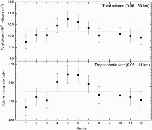
Table 2. Monthly averaged OCS total column and volume mixing ratio, with their errors, above Paris measured by the QualAir FTS (described in Section 2a) from March 2011 to March 2012.

Months	Total column (×10^15 molecules cm^−2)	Error (1σ) on column (×10^15 molecules cm^−2)	Tropospheric vmr (pptv)	Error on tropospheric vmr (pptv)
January	9.74	0.29	500.7	13.0
February	10.05	0.30	517.3	13.4
March	10.03	0.30	511.9	13.3
April	10.46	0.31	541.2	14.0
May	10.75	0.32	553.6	14.3
June	10.62	0.32	552.7	14.3
July	10.36	0.31	538.1	13.9
August	10.02	0.30	520.7	13.5
September	—^a	—	—	—
October	10.08	0.30	519.9	13.5
November	10.00	0.30	517.5	13.4
December	9.93	0.30	512.7	13.3

^aOnly one day of measurements is available for September, which is not representative of monthly averaging.

b Balloon-Borne Instruments

This study use data from balloon-borne measurements from three large balloon campaigns. The first was conducted from Teresina (5.1°S, 42.9°W) in northeastern Brazil in June 2008 with a SPIRALE flight on 9 June 2008. The second campaign was conducted from Esrange (Swedish Space Corporation) close to Kiruna, Sweden (67.9°N, 21.1°E). The SWIR balloon instrument flew on 14 August and the SPIRALE on 24 August 2009. The last campaign was also conducted from Esrange, with a SPIRALE instrument flight on 21 April 2011.

1 swir-balloon instruments

The SWIR balloon instrument is an extended version in the SWIR domain of the balloon-borne Infrared Atmospheric Sounding Interferometer (IASI) balloon instrument (Té et al., 2002). This instrument is an infrared remote sensing instrument based on a Fourier transform interferometer. The interferometer uses two InSb detectors to cover both thermal infrared (3–5 μm) and SWIR (1.8–2.4 µm) domains. In the nadir-looking configuration, the maximum optical path difference (OPD) is fixed at 10 cm. The SWIR balloon instrument observes the upwelling radiation that is composed of several contributions from surface emissions from the Earth, emission and absorption of atmospheric constituents, cloud emissions, and reflected solar radiation. Two reference sources on the optical head are used to perform an absolute calibration (Revercomb et al., 1988; Té, Jeseck, Pépin, & Camy-Peyret, 2009).

The first flight of the SWIR balloon instrument (SWIR01 flight) took place in the polar atmosphere and the instrument was flown above the Esrange–Kiruna region in Sweden (67.9°N, 21.1°E) on 14 August 2009 at 0926 utc and lasted 5 h 58 min. The first position of the gondola at float was 68.1°N, 21.0°E and the last position before balloon cut-off was 68.4°N, 20.6°E. The altitude at float varied around 34 km.

The Laboratoire de Physique Moléculaire pour l'Atmosphère et l'Astrophysique (LPMAA) Atmospheric Retrieval Algorithm (LARA; Té et al., 2002) is a radiative transfer model coupled with an inversion code to retrieve the total columns (from the surface to the gondola height of 34 km) of CO, O₃, OCS, CO₂, N₂O, and H₂O. For the OCS retrieval, the spectral window from 2065 to 2145 cm⁻¹ was selected for SWIR01, using the HITRAN 2012 database (Rothman et al., 2013). In addition to OCS, the contribution of six other atmospheric species, H₂O, CO₂, O₃, N₂O, CO, and CH₄, has been taken into account. The main interfering species in these spectral windows are H₂O, CO₂, O₃, and CO. For the other two constituents, the absorption signals are comparable to the noise level. OCS is retrieved from 0.32 km to 34 km for SWIR01, using the Université Pierre et Marie Curie (UPMC) two-dimensional (2D) model (Bekki & Pyle, 1992; Weisenstein & Bekki, 2006) profiles as vmr profiles. The error bars in Fig. 2 are the standard deviations of all retrieved columns during the flight.

Fig. 2 Pressure-corrected total column of OCS with error bars (standard deviation) versus latitude (°N). The ground-based (NDACC and other) and balloon-borne measurements from the Bruker IFS125HR interferometer, the MkIV instrument (orange, Toon, 1991) and the QualAir FTS instrument (red) are the weighted averages of several years with the minimum and maximum of each range shown by crosses and dashed lines. The other measurements are from Polarstern cruise campaigns measured by a Bruker 120M interferometer (Notholt et al., 2000; Xu, Bingemer, Georgii, Schmidt, & Bartell, 2001) and from the SWIR-balloon instrument from the Esrange balloon campaign (red, Té et al., 2002).

2 spirale instrument

The SPIRALE spectrometer has six tunable laser diodes for in situ measurements of trace gas species from the upper troposphere to the middle stratosphere (approximately 34 km height). A detailed description of the instrument can be found in a previous paper (Moreau et al., 2005). In brief, six mid-infrared region (3–8 μm) laser beams are passed between two mirrors spaced 3.50 m apart in a Herriott configuration multipass cell located at the extremities of a deployable mast below the gondola, leading to an average path length of 430.5 m. Several species, such as O₃, N₂O, CH₄, HCl, NO₂, HNO₃, and CO, were measured with high frequency sampling (approximately 1 Hz), which leads to a vertical resolution of a few metres (3 to 5 m), depending on the vertical velocity of the balloon. The overall uncertainties take into account the random and systematic errors, combined as the square root of their quadratic sum. The two main sources of random errors are the fluctuations of the laser background emission signal and the signal-to-noise ratio. At low altitudes (less than 20 km), the overall uncertainties make the same contribution. Systematic errors essentially originate from the laser line width (an intrinsic characteristic of the laser diode), which contributes more at lower pressures than at higher pressures (lower altitude). For OCS, the overall uncertainty is 3.3 ± 1.0% (1σ confidence level) below 18 km, increasing from 10.7 ± 3.0% at 18 km to 30% at 26 km and greater than 30% above 26 km. Absorption micro-windows for the three flights were 2056.1 to 2056.5 cm⁻¹, unperturbed by ozone or water absorption. The concentration of OCS was retrieved with the new HITRAN 2012 database (Rothman et al., 2013).

The following time sequences characterized the SPIRALE flights. During the night of 9 to 10 June 2008 in Brazil, measurements started at 2330 utc (i.e., 2030 local time) and the maximum altitude of 33.6 km (6.9 hPa) was reached at 0114 utc. The descent phase started at 0152 utc at 33.7 km and the measurements ended at 0535 utc at 16.9 km (95 hPa). For the second flight on the night of 24 to 25 August 2009 in Sweden, measurements started at 2050 utc (i.e., 2350 local time) and the maximum altitude of 34.1 km (6.9 hPa) was reached at 2230 utc. The descent phase started at 2326 utc at 33.7 km and the measurements ended at 0136 utc at 16.7 km (94 hPa). The third flight on 20 April 2011 in Sweden was again characterized by a slow ascent with measurements starting at 2100 utc at 8.6 km to 2330 utc at 33.3 km.

3 Results and discussion

a Column Variability

1 Seasonal variability above Paris

Figure 1 presents the monthly mean OCS total column above Paris and the tropospheric OCS vmr averaged from March 2011 to March 2012 measured by the QualAir FTS. Table 2 presents the values and the errors corresponding to the standard deviation used to produce Fig. 1. Seasonal patterns appear in the OCS data with a maximum in April–June (10.9 × 10¹⁵ molecules cm⁻² and 544 pptv) and a minimum in November–January (9.8 × 10¹⁵ molecules cm⁻² and 507 pptv). The variability of OCS with season is equal to 10% (peak-to-peak variation) in agreement with Griffith et al. (1998). The annual variation and the timing of the observed maximum are consistent with the study of Lejeune et al. (2011) at Jungfraujoch (NDACC station, 46.6°N). However, those authors observed a minimum during October–December with a peak-to-peak variation of 7.9%, whereas we found a minimum shifted to November–January. Similar periods are observed at Izana (28.30°N, NDACC station) as reported by Notholt and Bingemer (2006) with a minimum in October–December and an annual variation of 10%. However, a minimum during the November–January period, as in our work, was observed at Kitt Peak (32°N) (Rinsland et al., 2002). To sum up, a strong seasonal variation exists for many ground-based sites in the northern hemisphere, with a minimum occurring between October and January and a maximum between April and June (Notholt & Bingemer, 2006).

The seasonal variations are directly related to the natural sinks and sources of OCS (Kettle et al., 2002a). The amplitude of the variation depends on surface processes such as the imbalance between vegetation and soil uptakes and oceanic fluxes. The maximum in the total column occurs during the highest production of OCS (direct flux), DMS, and CS₂ (indirect flux) by biogenic processes in the ocean during late spring and the beginning of summer (Kettle et al., 2002a) and just before the maximum OCS uptake by land plants from July to September (Kettle et al., 2002b). The minimum period in October–January occurs during the lowest production by oceans and during less strong but still significant uptake by plants, soils, and by the OH reaction (Kettle et al., 2002a).

2 latitudinal variability

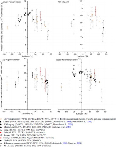
An update of the long-term OCS total column shows an annual increase lower than 0.79% (Montzka & Reimann, 2011). Consequently, for the rest of this study we assume a negligible interannual variation allowing us to compare measurements from different years. OCS total columns are extracted from the measurements from the SWIR balloon instrument at Esrange and from QualAir FTS measurements at the Paris station. These total columns are compared with other weighted average measurements (the weight of each measurement is relative to its standard deviation); OCS total column from NDACC stations (http://www.ndsc.ncep.noaa.gov/); the well-referenced Polarstern cruise campaigns (Notholt et al., 2000; Xu et al., 2001); and from other campaigns using the MkIV instrument at different latitudes.

Most of the measurements used in this study come from FTIR instruments to detect OCS, mostly in the same wavelength domain (2040 cm⁻¹ and 2080 cm⁻¹). A total of 19 measurement stations are used with 11 datasets coming from the MkIV instrument (Toon, 1991). The MkIV instrument uses the bands between 2041 and 2077 cm⁻¹ to detect OCS in the atmosphere. The measurements from the other stations use the same approach to derive OCS. All the datasets from the MkIV instrument use the new HITRAN database, which was updated in 2012 (Rothman et al., 2013). For the other stations that utilize HITRAN spectroscopic parameters before 2008, the columns were multiplied by 0.86, corresponding to the increase in the line strengths of OCS. All comparisons are shown in Fig. 2. The figure is divided into four panels according to the seasonal variation found in Section 3a1: January, February, and March (JFM); April, May, and June (AMJ); July, August, and September (JAS); and October, November, and December (OND). The total OCS columns plotted in Fig. 2 are scaled to sea level by multiplying the total column by the ratio of the standard pressure (1013 hPa) to the surface pressure observed at each station.

A latitudinal trend seems to appear in the OCS total columns whatever the season. The OCS total column decreases from tropical to polar latitudes from (10–11) × 10¹⁵ molecules cm⁻² to (6.5–9) × 10¹⁵ molecules cm⁻². The SWIR measurements from Esrange and the QualAir FTS measurement (red symbols in Fig. 2) are in accordance with the latitudinal trend observed within the uncertainties. Polarstern cruise campaigns highlight a maximum in the values near 20°N in the Atlantic Ocean (17°N, 21°W for JFM and 23°N, 30°W for OND). Bates, Lamb, Guenther, Dignon, and Stoiber (1992) show maximum oceanic sulphur emissions in a latitudinal band between 5°N and 20°N. In addition, over the Atlantic Ocean, the atmosphere is clearly affected by African and South American biomass burning leading to OCS emissions (Junkermann & Stockwell, 1999).

High latitudes seem to be more affected by seasonal variations. A seasonal variation of 14% is observed at Thule (76.53°N); a mean value of 10.5 × 10¹⁵ molecules cm⁻² without any significant variation for the six months of measurements (JFM and OND) is measured at latitudes between 20°S and 20°N. A minimum of 6.61 × 10¹⁵ molecules cm⁻² is observed at Thule during OND compared with the maximum value of 7.58 × 10¹⁵ molecules cm⁻² observed during AMJ. Barkley, Palmer, Boone, Bernath, and Suntharalingam (2008) observed the same phenomenon in the OCS vertical profile from ACE for different seasons at tropical latitudes (20°S–20°N), with OCS values remaining rather constant over the year.

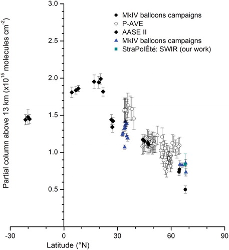
OCS has a long lifetime, resulting in quasi-uniformity of its vmr in the troposphere. Is the tendency in the total column also observed in the partial column above 13 km? Figure 3 shows the OCS partial column in the upper troposphere and lower stratosphere (UTLS) (above 13 km) for the campaigns using the SWIR-balloon instrument at Esrange compared with balloon campaigns using the MkIV instrument (SOLVE I and II, STRAT, and POLARIS; http://espoarchive.nasa.gov/) and several aircraft campaigns in which OCS was measured by FTIR (Polar Aura Validation Experiment (P-AVE) (Coffey & Hannigan, 2010) and the Airborne Arctic Stratospheric Expedition (AASE II; http://espoarchive.nasa.gov/)). All these datasets use either the HITRAN 2008 or 2012 database. The SOLVE I and II, P-AVE, and AASE II campaigns took place in December and JFM and are represented in black in Fig. 3, and the POLARIS, STRAT, and StraPolEte campaigns took place in June and JAS and are represented in blue. As for total column, a trend appears for the OCS column with latitude at altitudes above 13 km, from 0.5 × 10¹⁵ molecules cm⁻² at polar latitudes to 2.0 × 10¹⁵ molecules cm⁻² at tropical latitudes. This trend is also observed in the stratosphere and shows that tropical UTLS is composed of tropospheric young air transported from its local source compared with the polar stratosphere composed of older air coming mainly from the tropical stratosphere. As previously for the total column in the tropics, a maximum is found at 17°N in the Atlantic Ocean (17°N, 66°W, near the Dominican Republic). Again, this is a result of high oceanic emissions found at these latitudes (5°N–20°N) transported by convection as well as to African biomass burning transported over the Atlantic Ocean (Ricaud et al., 2007).

Fig. 3 OCS partial column above 13 km with error bars (representing the 1σ measurement precisions) versus latitude (°N) from several MkIV campaigns (STRAT, POLARIS, SOLVE I and II, and AASE II) (Toon, 1991; Toon, Blavier, Solario, & Szeto, 1993), aircraft P-AVE campaigns measured by the FTIR instrument (Coffey & Hannigan, 2010), and from the StraPolÉté balloon campaign measured by the SWIR instrument (dark cyan; Té et al., 2002). The values in blue (blue and dark cyan) are for campaigns occurring during June, July, and August and in black for campaigns occurring during January, February, and March.

b Vertical In Situ Measurements

1 vertical variability with latitude

Figure 4 shows, for the first time, high-resolution in situ OCS measurements at two different latitudes, tropical (5.1°S) and polar (67.9°N), measured by the SPIRALE instrument. These profiles correspond to the flights on 9 June 2008 at Teresina and 24 August 2009 and 20 April 2011 at Esrange. The thermal tropopause (WMO, 1957) was located at 16.9, 9.5, and 9.3 km on 9 June 2008, 24 August 2009, and 21 April 2011, respectively. Consequently, only the vertical profile at the tropical latitude contains values in the upper troposphere and, in particular, in the tropical tropopause layer (TTL) (Fueglistaler et al., 2009). The altitude of the TTL for the SPIRALE flight, identified by the solid blue line in Fig. 4, is 14.4 km to 18.0 km (Marécal et al., 2011). The transition from the TTL to the stratosphere is clearly seen by a decrease in the OCS vmr from more than 550 pptv to less than 500 pptv. The TTL is characterized by the transition from a pure tropospheric regime to a pure stratospheric regime. The bottom of the TTL is directly affected by the main convective outflow; consequently, the OCS vmr is almost constant with values comparable to those found in the troposphere. The upper TTL is not affected by convection; consequently, OCS sinks (photolysis, OH reaction) are predominant.

Fig. 4 SPIRALE measurements of OCS volume mixing ratios (in ppt) with error bars on 9 June 2008 (filled blue circles) above Teresina, Brazil (5.1°S, 42.9°W) on 24 August 2009 (open red circles) and 20 April 2011 (filled black circles) above Esrange, Sweden (67.9°N, 21.1°E). The thermal tropopause (Tp) and the tropical tropopause layer (TTL) top and bottom are represented by a solid blue line and by blue dashed lines, respectively, for the flight at tropical latitudes on June 2008.

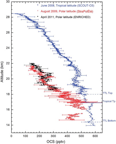
The profiles show the OCS vertical distribution well. The OCS mixing ratios at tropical latitudes are approximately constant between 14 and 17 km altitude with values of 540 to 570 pptv, which then start to decrease above the thermal tropopause (Tp) from 550 pptv at a height of 17 km to 34 pptv at a height of 28.5 km. Indeed, OCS is mainly destroyed in the stratosphere by photolysis (Notholt & Bingemer, 2006) with a maximum absorption at λ < 250 nm (Molina, Lamb, & Molina, 1981). According to DeMore et al. (1997), at λ < 250 nm, the actinic flux is maximum at altitudes higher than 20 km. The OCS mixing ratio behaviour at polar latitudes is similar to that at tropical latitudes. Because of instrumental problems, the polar profile is more scattered than the tropical one. At polar latitudes we observe a decrease in the OCS vmr with altitude, from 420 ± 100 pptv at altitudes lower than 17 km and a decrease from 460 pptv to 150 pptv at 22 km. During the STRAT campaign in July 1996, the MkIV instrument observed a similar behaviour, with OCS vmr values constant at 440 pptv below 14 km (Leung et al., 2002) and a decrease to 120 pptv at 22 km.

The latitudinal variation in OCS in the stratosphere is significant, with a large vmr increase from about 150 pptv to about 300 pptv between the tropopause and 22 km. Barkley et al. (2008) observed a similar difference, of about 250 pptv, in the OCS vmr between tropical and polar latitudes using data from the ACE satellite. This phenomenon is also observed in the OCS partial column explained in Section 3a (latitudinal variability). This is due to global atmospheric transport regulating the amount of OCS in the polar stratosphere. OCS tropospheric air reaches the stratosphere at tropical latitudes. Subsequently, OCS is transported poleward by the Brewer-Dobson circulation while being photodissociated. Tropical and mid-latitude poleward intrusions of tropospheric air into the extratropical stratosphere are also possible stratospheric sources of OCS (Krysztofiak et al., 2012; Roiger et al., 2011). This could explain the various OCS vmr enhancements in the polar profiles.

2 comparisons with ace satellite data

The ACE mission on board the Canadian SCISAT satellite (Bernath et al., 2005) was launched 12 August 2003. Using the solar occultation technique, two instruments measure the vertical profiles of atmospheric constituents from the troposphere to the lower mesosphere. For this study, we use the OCS version 3.0 (v.3.0) of the vmr profiles from the ACE Fourier Transform Spectrometer (ACE-FTS). A total of thirteen micro-windows is used for the OCS ACE-FTS v. 3.0 vmr retrievals, positioned at 1950.10 cm⁻¹ for the first and between 2039.01 cm⁻¹ and 2057.52 cm⁻¹ for the others. In order to compare ACE-FTS and SPIRALE data we must take into account the difference in the vertical resolution of these two instruments. Indeed, ACE-FTS data have a vertical resolution of 2–6 km whereas that of SPIRALE data is on the order of a few metres. For comparison, we use the ACE-FTS retrieved results which are interpolated onto a 1 km grid from 0.5 km to 149.5 km. A weighting triangular function of 3 km at the base is applied to SPIRALE data after interpolation onto a 5 m grid. Consequently, we have truncated the bottom and top of the SPIRALE profile from 1.5 km.

As explained in Section 3a (latitudinal variability), we assume a negligible OCS variation between 2003 (start date of the ACE measurements) and the year of our SPIRALE balloon flights (i.e., 2008 and 2009). Moreover, as seen in Section 3a1, there is a seasonal trend in the OCS vmr. Consequently, for comparisons of ACE-FTS results with SPIRALE results at Teresina in June 2008, we use OCS profiles from April to June and for comparisons at Esrange in August 2009, we use OCS profiles from July to September and only those profiles obtained above land (balloon flights occurred above land). There are few ACE profiles available at tropical latitudes thus, for the comparison at Teresina, we used six profiles (between 2004 and 2007) acquired at 5 ± 6°S and 43(+20, −10)°W. For the comparison at Kiruna, we used 56 profiles (between 2004 and 2011) acquired at 67.9 ± 6°N and 21.1 ± 10°E.

Figure 5 (left panels) shows the comparisons of SPIRALE OCS measurements and the weighted average (weight of each measurement relative to its standard deviation) of the ACE-FTS OCS profiles. Figure 5 (right panels) shows the difference between the SPIRALE and ACE average (SPIRALE-ACE (%)) compared with the mean value with error bars.

Fig. 5 Left panels: SPIRALE measurements of OCS volume mixing ratios (in pptv) with error bars (red triangles) compared with the weighted average (weight of each measurement relative to its 1σ error) of the ACE-FTS OCS profiles with error bars (1σ) (black squares). The grey dashed lines represent the spread (minimum and maximum values found in all ACE profiles). Right panels: Percentage differences between the SPIRALE and ACE-FTS data with error bars. The vertical red line is drawn only to mark a zero difference. Top panels: Comparisons for the SPIRALE flight on 9 June 2008 at Teresina, Brazil. Bottom panels: Comparisons for the SPIRALE flight on 24 August 2009 at Esrange, Sweden.

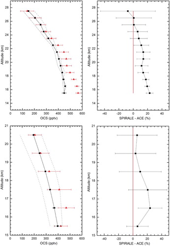
For tropical latitudes, at altitudes lower than 22.5 km, ACE-FTS underestimates OCS values compared with SPIRALE. The differences between the SPIRALE and ACE values indicate a bias between 15 and 20%. For altitudes higher than 22.5 km, at Teresina, the SPIRALE and ACE-FTS values are in very good agreement (within 10%).

At polar latitudes, at Esrange, the SPIRALE and ACE-FTS values are also in very good agreement (within 11%) taking into account the uncertainties in both instruments, except at 16.5 km where the ACE-FTS underestimates the OCS values compared with the SPIRALE values with a bias of 20%.

Velazco et al. (2011, their Fig. 18) show a similar bias of 15% between ACE-FTS and MkIV OCS profiles for altitudes between 12 and 23 km (350–550 K) at 35°N.

3 stratospheric lifetime

Plumb and Ko (1992) highlighted the use of tracer-tracer correlations to determine the atmospheric lifetime of species. Simultaneous N₂O measurements were performed by SPIRALE in the tropical and polar regions. Similar to OCS, N₂O has purely tropospheric sources (Seinfeld & Pandis, 2006) and possesses a long lifetime compared with horizontal and vertical air motions. The lower stratosphere (below 22 km) correlation between OCS and N₂O is linear, and the relationship between their atmospheric lifetimes is represented by the following equation:(4) where τ represents the stratospheric lifetime, vmr the tropospheric volume mixing ratio, and A the slope of the correlation (Plumb & Ko, 1992).

Because of the absence of data below 18 km in the OCS profile at polar latitudes on 21 April 2011, the correlation between OCS and N₂O in the lower stratosphere cannot be plotted and no lifetime has been calculated for this date.

Figure 6a represents the correlation between N₂O and OCS in the lower stratosphere at tropical latitudes in 2008 and Fig. 6b at polar latitudes in 2009 from SPIRALE measurements. Both linear correlations lead to a coefficient of determination, r², greater than 0.75.

Fig. 6 Correlation between N₂O and OCS from SPIRALE volume mixing ratio in situ measurements in the lower stratosphere (below 22 km): (a) 9 June 2008 above Teresina, Brazil (5.1°S, 42.9°W) and (b) 24 August 2009 above Esrange, Sweden (67.9°N, 21.1°E).

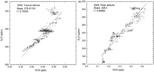
We use an N₂O lifetime of 117 ± 20 years from Montzka and Fraser (2003) and a mean tropospheric mixing ratio of 311 ± 8 ppbv for N₂O and 550 ± 40 pptv for OCS from SPIRALE measurements to calculate the OCS stratospheric lifetime at tropical and polar latitudes. We find a lifetime of 68 ± 20 years at polar latitudes and 58 ± 14 years for tropical latitudes, which leads to a mean global stratospheric lifetime of 63 ± 15 years. Actinic fluxes for λ < 250 nm (OCS photodissociation) and for altitudes higher than 20 km show a difference with latitude (Finlayson-Pitts & Pitts, 2000). Indeed, for the same solar time and months (here June and August), the solar zenith angle is smaller at tropical latitudes than at polar latitudes and for λ < 250 nm the actinic fluxes increase with decreasing solar zenith angles. Consequently, OCS undergoes stronger photolysis at tropical latitudes and has a lower stratospheric lifetime.

Using the correlation with CFCl₃ (lifetime of 55 years), Engel and Schmidt (1994) found an OCS stratospheric lifetime of 69 ± 28 years at latitudes higher than 43°N from measurements taken at Kiruna (68°N) and Aire sur l'Adour (43°N). Using correlations with CF₂Cl₂ and CFCl₃, Barkley et al. (2008) found a global OCS stratospheric lifetime of 64 ± 21 years. These values are consistent with our global value. The value found by Engel and Schmidt (1994) is consistent with our polar value. Unfortunately, Barkley et al. (2008) did not estimate OCS lifetime at latitudes between 20°N and 20°S, so no comparison is possible with our OCS lifetime for tropical latitudes (Teresina).

The correlations between N₂O and OCS from the ACE-FTS data used in Section 3b2 in polar regions and from the MkIV measurements during several campaigns (SOLVE I and II) in the Kiruna region are used to extract the OCS lifetime in the polar region. These results are compared with our lifetime from SPIRALE measurements in the polar region and the other lifetimes found by Engel and Schmidt (1994) and Barkley et al. (2008) at polar latitudes. Table 3 shows these comparisons. All the lifetimes found in the polar region are consistent and allow us to establish an OCS lifetime of 71 ± 10 years by taking into account the overall uncertainties in the polar region.

Table 3. OCS lifetimes (years) in the polar region from SPIRALE measurements, from ACE-FTS measurements (data from Section 3b2) and from MkIV measurements (http://mark4sun.jpl.nasa.gov/m4data.html) compared with the study by Engel and Schmidt (1994) and Barkley et al. (2008).

	Engel and Schmidt (1994)	Barkley et al. (2008)	ACE-FTS	MkIV	SPIRALE
Lifetime (years)	69 ± 28^a	76 ± 32^a	70 ± 16^b	74 ± 24^b	68 ± 20^b

^aCFC-12/OCS correlation.

^bN₂O/OCS correlation.

We can calculate the stratospheric OCS sink by dividing the total OCS mass in the atmosphere, 5.86 × 10¹² g (inferred from the total atmospheric mass of 5.148 × 10²¹ g (Trenberth & Smith, 2005) and our tropospheric OCS vmr) by our global OCS lifetime. We find a global stratospheric sink of 92 ± 26 Gg OCS y⁻¹, corresponding to 49 ± 14 Gg S y⁻¹. Table 4 shows a comparison between our OCS stratospheric sink values and several values from the literature. Our range of values is in general agreement with the average 50 ± 15 (1σ) Gg S y⁻¹ of OCS stratospheric sinks found in previous studies.

Table 4. OCS stratospheric sink (Gg S y⁻¹) comparison with previous studies.

	Crutzen (1976)	Turco, Whitten, Toon, Pollack, and Hamill (1980)	Crutzen and Schmailzl (1983)	Engel and Schmidt (1994)	Chin and Davis (1995)	Weisenstein et al. (1997)	Barkley et al. (2008)	This work
OCS Stratospheric sink (Gg S y^−1)	50	80	43	49 ± 20	30	49	50 ± 16	49 ± 14

4 Conclusions and perspectives

Carbonyl sulphide (OCS) is the most abundant sulphur-containing compound in the atmosphere. Because of its long lifetime, OCS can easily reach the stratosphere and is, with SO₂, the precursor of sulphate aerosols. Consequently, it is a key species for understanding the heterogeneous chemistry of stratospheric ozone depletion.

A seasonal variation is extracted from ground-based FTS measurements from the QualAir platform at Jussieu campus in Paris. A maximum value in the total column and the tropospheric mean vmr are found in April–June and a minimum value in November–January with a peak-to-peak variability of 10%.

Total column measurements from QualAir FTS measurements above Paris and SWIR balloon-borne instruments are compared with several measurements, from the MkIV instrument, NDACC stations measurements, ship measurements, and balloon-borne measurements, to highlight OCS variability with latitude. The OCS total column decreases with increasing latitude. The variability is also found for the partial column above 13 km showing the atmospheric OCS transport from the tropical troposphere into the tropical stratosphere and then into the polar stratosphere. The OCS total columns show a more pronounced seasonal variability at polar latitudes than at tropical latitudes.

The first high-resolution vertical profile of OCS at two different latitudes is presented in this paper. The SPIRALE balloon-borne instrument flew over the tropical region (5.1°S, Teresina, Brazil) on 9 June 2008 and over the polar Arctic region (67.9°N, Esrange, Sweden) on 24 August 2009. The OCS vertical dependence is similar for both latitudes with a significant decrease in OCS vmr above 20 km. The OCS profiles are also compared with non-coincident ACE satellite measurements and are in good agreement at polar latitudes with a bias of 15–20% at tropical latitudes for altitudes lower than 22 km.

Using the correlation between OCS and N₂O from SPIRALE, OCS stratospheric lifetime is determined accurately. We found a lifetime of 68 ± 20 years at polar latitudes and 58 ± 14 years at tropical latitudes which leads to a mean global stratospheric lifetime of 63 ± 15 years. Global lifetimes are used to determine the stratospheric sink of OCS. In the lower stratosphere, the OCS stratospheric degradation produces 49 ± 14 Gg S y⁻¹.

Further investigations should include modelling studies of the contribution of OCS to the stratospheric aerosol burden.

Acknowledgements

The authors would like to thank the Laboratoire de Physique et Chimie de l'Environnement et de l'Espace (LPC2E) technical team (L. Pomathiod, B. Gaubicher, G. Chalumeau, B. Coûté, T. Vincent, F. Savoie. G. Jannet, and S. Chevrier) for the SPIRALE instrument preparation, the LPMAA technical team (I. Pépin, C. Rouillé, and P. Marie-Jeanne), the SWIR-balloon instruments preparation, the CNES balloon launching team, and the Swedish Space Corporation at Esrange for successful field operations. The instrumental funding for the QualAir FTS was supported by the University Paris VI (Université Pierre et Marie Curie). The Ether database (Pôle thématique du CNES-INSU-CNRS) and the CNES sous-direction Ballon are partners of the project. This work was supported by the European integrated project SCOUT-O3 (GOCE-CT-2004-505390), the European Space Agency (ESA) as part of the Envisat validation program, the French national Les Enveloppes Fluides et l'Environnement / Institut National des Sciences de l'Univers (LEFE/INSU) project UTLS Tropicale, by the French national Labex Étude des géofluides et des VOLatils–Terre, Atmosphère et Interfaces - Ressources et Environnement (VOLTAIRE) (ANR-10-LABX-100-01), by the StraPolÉté project funded by the Agence Nationale de la Recherche (ANR-BLAN08-1_31627), the Centre National d’Études Spatiales (CNES), and the Institut polaire français Paul Emile Victor (IPEV), and by the ENRICHED project funded by the CNES, INSU-CNRS, and IPEV. The Atmospheric Chemistry Experiment (ACE), also known as SCISAT, is a Canadian-led mission mainly supported by the Canadian Space Agency. The data used in this publication were obtained as part of the Network for the Detection of Atmospheric Composition Change (NDACC) and are publicly available (http://www.ndacc.org). Part of this work was performed at the Jet Propulsion Laboratory, California Institute of Technology, under contract to NASA. The authors also wish to thank J. Notholt and O. Schrems for their data from the Polarstern campaign. We thank M. Coffey and J. Hannigan for their results from the P-AVE campaign.

References

- Barkley, M. P., Palmer, P. I., Boone, C. D., Bernath, P. F., & Suntharalingam, P. (2008). Global distributions of carbonyl sulfide in the upper troposphere and stratosphere. Geophysical Research Letters, 35, L14810. doi:10.1029/2008GL034270
- Barletta, B., Meinardi, S., Simpson, I. J., Atlas, E. L., Beyersdorf, A. J., Baker, A. K., … Blake, D. R. (2009). Characterization of volatile organic compounds (VOCs) in Asian and north American pollution plumes during INTEX-B: Identification of specific Chinese air mass tracers. Atmospheric Chemistry and Physics, 9, 5371–5388. doi:10.5194/acp-9-5371-2009
- Bates, T. S., Lamb, B. K., Guenther, A., Dignon, J., & Stoiber, R. E. (1992). Sulfur emissions to the atmosphere from natural sources. Journal of Atmospheric Chemistry, 14, 315–337. doi: 10.1007/BF00115242
- Bekki, S., & Pyle, J. A. (1992). 2-D assessment of the impact of aircraft sulphur emissions on the stratospheric sulphate aerosol layer. Journal of Geophysical Research, 97, 15839–15847. doi:10.1029/92JD00770
- Bernath, P., McElroy, C. T., Abrams, M. C., Boone, C. D., Butler, M., Camy-Peyret, C., … Zo, J. (2005). Atmospheric Chemistry Experiment (ACE): Mission overview. Geophysical Research Letters, 32, L15S01. doi:10.1029/2005GL022386
- Blake, N. J., Campbell, J. E., Vay, S. A., Fuelberg, H. E., Huey, L. G., Sachse, G., … Blake, D. R. (2007). Carbonyl sulfide (OCS): Large-scale distributions over North America during INTEX-NA and relationship to CO2. Journal of Geophysical Research, 113, D09S90. doi:10.1029/2007JD009163
- Blake, N. J., Streets, D. G., Woo, J.-H., Simpson, I. J., Green, J., Meinardi, S., … Blake, D. R. (2004). Carbonyl sulfide and carbon disulfide: Large-scale distributions over the western Pacific and emissions from Asia during TRACE-P. Journal of Geophysical Research, 109, D15S05. doi:10.1029/2003JD004259
- Chin, M., & Davis, D. D. (1993). Global sources and sinks of OCS and CS2 and their distributions. Global Biogeochemical Cycles, 7, 321–337. doi: 10.1029/93GB00568
- Chin, M., & Davis, D. D. (1995). A reanalysis of carbonyl sulfide as a source of stratospheric background sulfur aerosol. Journal of Geophysical Research, 100(D5), 8993–9005. doi:10.1029/95JD00275
- Clough, S. A., Shephard, M. W., Mlawer, E. J., Delamere, J. S., Lacono, M. J., Cady-Pereira, K., … Brown, P. D. (2005). Atmospheric radiation transfer modelling: A summary of the AER codes, short communication. Journal of Quantitative Spectroscopy & Radiative Transfer, 91, 233–244. doi: 10.1016/j.jqsrt.2004.05.058
- Coffey, M. T., & Hannigan, J. W. (2010). The temporal trend of stratospheric carbonyl sulphide. Journal of Atmospheric Chemistry, 67, 61–70. doi:10.1007/s10874-011-9203-4
- Crutzen, P. J. (1976). The possible importance of CSO for the sulfate layer of the stratosphere. Geophysical Research Letters, 3, 73–76. doi: 10.1029/GL003i002p00073
- Crutzen, P. J., & Schmailzl, U. (1983). Chemical budget of the atmosphere. Planetary and Space Science, 31, 1009–1032. doi: 10.1016/0032-0633(83)90092-2
- DeMore, W. B., Sander, S. P., Golden, D. M., Hampson, R. F., Kurylo, M. J., Howard, C. J., … & Molina, M. J. (1997). Chemical kinetics and photochemical data for use in stratospheric modelling (JPL Publication 97-4). Pasadena, CA: Jet Propulsion Laboratory.
- Deutscher, N. M., Jones, N. B., Griffith, D. W. T., Wood, S. W., & Murcray, F. J. (2006). Atmospheric carbonyl sulfide (OCS) variation from 1992–2004 by ground-based solar FTIR spectrometry. Atmospheric Chemistry and Physics Discussions, 6, 1619–1636. doi:10.5194/acpd-6-1619-2006
- Engel, A., & Schmidt, U. (1994). Vertical profile measurements of carbonyl sulfide in the stratosphere. Geophysical Research Letters, 21, 2219–2222. doi: 10.1029/94GL01461
- Finlayson-Pitts, B. J., & Pitts, J. N. (2000). Chemistry of the upper and lower atmosphere – theory, experiments and applications, chapter 3, p. 68. San Diego: Academic Press.
- Fueglistaler, S., Dessler, A. E., Dunkerton, T. J., Folkins, I., Fu, Q., & Mote, P. W. (2009). Tropical tropopause layer. Reviews of Geophysics, 47, RG1004. doi:10.1029/2008RG000267
- Griffith, D. W. T., Jones, N. B., & Matthews, W. A. (1998). Interhemispheric ratio and annual cycle of carbonyl sulfide (OCS) total column from ground-based solar FTIR spectra. Journal of Geophysical Research, 103(D7), 8447–8454. doi:10.1029/97JD03462
- Harrigan, D. L., Fuelberg, H. E., Simpson, I. J., Blake, D. R., Carmichael, G. R., & Diskin, G. S. (2011). Anthropogenic emissions during Arctas-A: Mean transport characteristics and regional case studies. Atmospheric Chemistry and Physics, 11, 8677–8701. doi:10.5194/acp-11-8677-2011
- Hase, F., Hannigan, J. W., Coffey, M. T., Goldman, A., Höpfner, M., Jones, N. B., … & Wood, S. W. (2004). Intercomparison of retrieval codes used for the analysis of high-resolution, ground-based FTIR measurements. Journal of Quantitative Spectroscopy & Radiative Transfer, 87, 25–52. doi: 10.1016/j.jqsrt.2003.12.008
- Junkermann, W., & Stockwell, W. R. (1999). On the budget of photooxidants in the marine boundary layer of the tropical South Atlantic. Journal of Geophysical Research, 104(D7), 8039–8046. doi:10.1029/1998JD100060
- Kettle, A. J., Kuhn, U., von Hobe, M., Kesselmeier, J., & Andreae, M. O. (2002a). Global budget of atmospheric carbonyl sulfide: Temporal and spatial variations of the dominant sources and sinks. Journal of Geophysical Research, 107, 4658. doi:10.1029/2002JD002187
- Kettle, A. J., Kuhn, U., von Hobe, M., Kesselmeier, J., Liss, P. S., & Andreae, M. O. (2002b). Comparing forward and inverse models to estimate the seasonal variation of hemisphere-integrated fluxes of carbonyl sulphide. Atmospheric Chemistry and Physics, 2, 343–361. doi:10.5194/acp-2-343-2002
- Krysztofiak, G., Thiéblemont, R., Huret, N., Catoire, V., Té, Y., Jégou, F., … Camy-Peyret, C. (2012). Detection in the summer polar stratosphere of air plume pollution from East Asia and North America by balloon-borne in situ CO measurements. Atmospheric Chemistry and Physics, 12, 11889–11906. doi:10.5194/acp-12-11889-2012
- Lejeune, B., Mahieu, E., Suntharalingam, P., Duchatelet, P., Servais, C., & Demoulin, P. (2011). Trend evolution and seasonal variation of tropospheric and stratospheric carbonyl sulfide (OCS) above Jungfraujoch. EGU General Assembly 2011, Vol. 13, EGU2011-3536.
- Leung, F. T., Colussi, A. J., Hoffmann, M. R., & Toon, G. C. (2002). Isotopic fractionation of carbonyl sulfide in the atmosphere: Implications for the source of background stratospheric sulfate aerosol. Geophysical Research Letters, 29(10). doi:10.1029/2001GL013955
- Marécal, V., Krysztofiak, G., Mébarki, Y., Catoire, V., Lott, F., Attié, J.-L., … Robert, C. (2011). Impact of deep convection on the tropical tropopause layer composition in equatorial Brazil. Atmospheric Chemistry and Physics Discussions, 11, 16147–16183. doi:10.5194/acpd-11-16147-2011
- Molina, L. T., Lamb, J. J., & Molina, M. J. (1981). Temperature dependent UV absorption cross sections for carbonyl sulfide. Geophysical Research Letters, 8(9), 1008–1011. doi:10.1029/GL008i009p01008
- Montzka, S. A., & Fraser, P. J. (2003). Controlled substances and other source gases. In Scientific Assessment of Ozone Depletion: 2002 (Chapter 1, Report No. 47). Geneva: Global Ozone Research and Monitoring Project, World Meteorological Organization.
- Montzka, S. A., & Reimann, S. (2011). Ozone-Depleting Substances (ODSs) and related chemicals. In Scientific Assessment of Ozone Depletion: 2010 (Chapter 1, Report No. 52). Geneva: Global Ozone Research and Monitoring Project, World Meteorological Organization.
- Moreau, G., Robert, C., Catoire, V., Chartier, M., Camy-Peyret, C., Huret, N., … Chalumeau, G. (2005). A multispecies in situ balloon-borne experiment with six tunable diode laser spectrometers. Applied Optics, 44(28), 5972–5989. doi: 10.1364/AO.44.005972
- Notholt, J., & Bingemer, H. (2006). Precursor gas measurements. SPARC (Report No. 4, Chapter 2, pp. 29–76). Toronto: World Climate Research programme - 124, WMO/TD No.1295, SPARC IPO.
- Notholt, J., Kuang, Z., Rinsland, C. P., Toon, G. C., Rex, M., Jones, N., … Schrems, O. (2003). Enhanced upper tropical tropospheric COS: Impact on the stratospheric aerosol layer. Science, 300, 307–310. doi:10.1126/science.1080320
- Notholt, J., Toon, G. C., Rinsland, C. P., Pougatchev, N. S., Jones, N. B., Connor, B. J., … Schrems, O. (2000). Latitudinal variations of trace gas concentrations in the free troposphere measured by solar absorption spectroscopy during a ship cruise. Journal of Geophysical Research, 105(D1), 1337–1349. doi:10.1029/1999JD900940
- Plumb, R. A., & Ko, M. K. W. (1992). Interrelationships between mixing ratios of long-lived stratospheric constituents. Journal of Geophysical Research, 97, 10145–10156. doi: 10.1029/92JD00450
- Revercomb, H. E., Buijs, H., Howell, H. B., LaPorte, D. D., Smith, W. L., & Sromovsky, L. A. (1988). Radiometric calibration of IR Fourier transform spectrometers: Solution to a problem with the High-Resolution Interferometer Sounder. Applied Optics, 27, 3210–3218. doi: 10.1364/AO.27.003210
- Ricaud, P., Barret, B., Attié, J.-L., Motte, E., Le Flochmoën, E., Teyssèdre, H., … Pommereau, J.-P. (2007). Impact of land convection on troposphere-stratosphere exchange in the tropics. Atmospheric Chemistry and Physics, 7, 5639–5657. doi:10.5194/acp-7-5639-2007
- Rinsland, C. P., Goldman, A., Mahieu, E., Zander, R., Notholt, J., Jones, N. B., … Chiou, L. S. (2002). Ground-based infrared spectroscopic measurements of carbonyl sulfide: Free tropospheric trends from a 24-year time series of solar absorption measurements. Journal of Geophysical Research, 107(D22), 4657. doi:10.1029/2002JD002522
- Roiger, A., Schlager, H., Schäfler, A., Huntrieser, H., Scheibe, M., Aufmhoff, H., … Arnold, F. (2011). In-situ observation of Asian pollution transported into the Arctic lowermost stratosphere. Atmospheric Chemistry and Physics, 11, 10975–10994. doi: 10.5194/acp-11-10975-2011
- Rothman, L. S., Gordon, I. E., Babikov, Y., Barbe, A., Benner, D. C., Bernath, P. F., … Wagner, G. (2013). The HITRAN 2012 molecular spectroscopic database. Journal of Quantitative Spectroscopy & Radiative Transfer, 130, 4–50. doi: 10.1016/j.jqsrt.2013.07.002
- Rothman, L. S., Gordon, I. E., Barbe, A., Benner, D. C., Bernath, P. F., Birk, M., … Vander Auwera, J. (2009). The HITRAN 2008 molecular spectroscopic database. Journal of Quantitative Spectroscopy & Radiative Transfer, 110, 533–572. doi: 10.1016/j.jqsrt.2009.02.013
- Sander, S. P., Friedl, R. P., Abbatt, J. P. D., Barker, J. R., Burkholder, J. B., Golden, D. M, … Orkin, V. L. (2011). Chemical kinetics and photochemical data for use in atmospheric studies evaluation number 17, JPL Publication 10-6. Pasadena, CA: National Aeronautics and Space Administration, Jet Propulsion Laboratory, California Institute of Technology.
- Seinfeld, J. H., & Pandis, S. N. (2006). Atmospheric chemistry and physics: From air pollution to climate change, chapter 7, p. 35. Second edition. New York: John Wiley & Sons Ed, Inc.
- Simpson, I. J., Blake, N. J., Barletta, B., Diskin, G. S., Fuelberg, H. E., Gorham, K., … Blake, D. R. (2010). Characterization of trace gases measured over Alberta oil sands mining operations: 76 speciated C2-C10 volatile organic compounds (VOCs), CO2, CH4, CO, NO, NO2, NOy, O3 and SO2. Atmospheric Chemistry and Physics, 10, 11931–11954. doi:10.5194/acp-10-11931-2010
- Té, Y., Jeseck, P., Camy-Peyret, C., Payan, S., Perron, G., & Aubertin, G. (2002). Balloonborne calibrated spectroradiometer for atmospheric nadir sounding. Applied Optics, 41, 6431–6441. doi: 10.1364/AO.41.006431
- Té, Y., Jeseck, P., Dieudonné, E., Hase, F., Hadji-Lazaro, J., Clerbaux, C., … Camy-Peyret, C. (2012). Carbon monoxide urban emission monitoring: A ground-based FTIR case study. Journal of Atmospheric and Oceanic Technology, 29(7). doi:10.1175/JTECH-D-11-00040.1
- Té, Y., Jeseck, P., Payan, S., Pépin, I., & Camy-Peyret, C. (2010). The Fourier transform spectrometer of the Université Pierre and Marie Curie University QualAir platform. Review of Scientific Instruments, 81, 103102. doi:10.1063/1.3488357
- Té, Y., Jeseck, P., Pépin, I., & Camy-Peyret, C. (2009). A method to retrieve blackbody temperature errors in the two points radiometric calibration. Infrared Physics & Technology, 52, 187–192. doi:10.1016/j.infrared.2009.07.003
- Toon, G. C. (1991). The JPL MkIV Interferometer. Optics & Photonics News, 2, 19–21. doi: 10.1364/OPN.2.10.000019
- Toon, G. C., Blavier, J.-F., Solario, J. N., & Szeto, J. T. (1993). Airborne observation of the composition of the 1992 tropical stratosphere by FTIR solar absorption spectrometry. Geophysical Research Letters, 20, 2503–2506. doi: 10.1029/93GL01962
- Trenberth, K. E., & Smith, L. (2005). The mass of the atmosphere: A constraint on global analyses. Journal of Climate, 18, 864–875. doi: 10.1175/JCLI-3299.1
- Turco, R. P., Whitten, R. C., Toon, O. B., Pollack, J. B., & Hamill, P. (1980). OCS, stratospheric aerosols and climate. Nature, 283, 283–286. doi: 10.1038/283283a0
- Velazco, V. A., Toon, G. C., Blavier, J.-F. L., Kleinböhl, A., Manney, G. L., Daffer, W. H., … Boone, C. (2011). Validation of the Atmospheric Chemistry Experiment by noncoincident MkIV balloon profiles. Journal of Geophysical Research, 116, D06306. doi:10.1029/2010JD014928
- Vernier, J.-P., Thomason, L. W., Pommereau, J.-P., Bourassa, A., Pelon, J., Garnier, A., … Vargas, F. (2011). Major influence of tropical volcanic eruptions on the stratospheric aerosol layer during the last decade. Geophysical Research Letters, 38, L12807. doi:10.1029/2011GL047563
- Weisenstein, D., & Bekki, S. (2006). Modeling of stratospheric aerosols. SPARC (Report No. 4, Chapter 6, pp. 219–319). Toronto: World Climate Research programme - 124, WMO/TD No.1295, SPARC IPO.
- Weisenstein, D. K., Yue, G. K., Ko, M. K. W., Sze, N. D., Rodriguez, J. M., & Scott, C. J. (1997). A two-dimensional model of sulfur species and aerosol. Journal of Geophysical Research, 102, 13019–13035. doi: 10.1029/97JD00901
- Wilson, J. C., Lee, S.-H., Reeves, J. M., Brock, C. A., Jonsson, H. H., Lafleur, B. G., … Moore, F. (2008). Steady-state aerosol distributions in the extra- tropical, lower stratosphere and the processes that maintain them. Atmospheric Chemistry and Physics, 8, 6617–6626. doi:10.5194/acp-8-6617-2008
- WMO (World Meteorological Organization). (1957). Meteorology: A three-dimensional science, 4, pp. 134–138. Geneva, Switzerland: WMO Bull.
- Xu, X., Bingemer, H. G., Georgii, H.-W., Schmidt, U., & Bartell, U. (2001). Measurements of carbonyl sulfide (COS) in surface seawater and marine air, and estimates of the air-sea flux from observations during two Atlantic cruises. Journal of Geophysical Research, 106, 3491–3502. doi:10.1029/2000JD900571