Sea-Ice Freeze-up Forecasts with an Operational Ocean Observatory

ABSTRACT

The evaluation of a new method for forecasting freeze-up at the eastern end of the Northwest Passage, a principal gateway into the Canadian High Arctic, is presented. The technique uses real-time data from a novel ocean observatory that combines acoustic, cable, and satellite communications technology to provide year-round bihourly data. The basis for the predictive capability comes from a previous analysis of a decade-long time series of instrumented mooring data collected in the area, which demonstrated a strong link between late summer upper ocean salinity and the timing of freeze-up there. Using real-time data from the observatory and this previously established relationship, accurate predictions of the timing of freeze-up in 2012 and 2013 with lead times of four weeks and two weeks, respectively, are presented. This unique forecasting capability points to the enhanced value of real-time data systems when these systems are located where previously collected long time series monitoring has revealed key relationships in the marine environment.

RÉSUMÉ

[Traduit par la rédaction] Nous présentons l’évaluation d'une nouvelle méthode de prévision de prise des glaces à l'extrémité est du passage du Nord-Ouest, l'un des principaux points d'accès à l'Arctique canadien septentrional. La méthode se fonde sur les données en temps réel d'un nouvel observatoire océanique qui combine des techniques de communication acoustiques, par câble et satellitaires pour fournir des données bihoraires tout au long de l'année. La capacité prévisionnelle s'appuie sur l'analyse précédente d'un ensemble chronologique de données provenant d'instruments ancrés dans la région depuis une décennie et qui a mis en lumière une relation étroite entre la salinité de la surface océanique à la fin de été et le moment de la prise des glaces à cet endroit. En utilisant les données en temps réel de l'observatoire et cette relation précédemment établie, nous présentons des prévisions du moment de la prise des glaces en 2012 et 2013, pour des termes de quatre semaines et deux semaines, respectivement. Cette capacité prévisionnelle particulière fait entrevoir une valeur ajoutée aux systèmes de données en temps réel quand ceux-ci sont situés là où de longues séries chronologiques recueillies précédemment révèlent des relations clés dans l'environnement marin.

KEYWORDS:

• sea ice
• ocean observatory
• forecasting
• freeze-up
• interannual variability

1 Introduction

As the observed trend of declining Arctic sea ice continues, the prospect of increased ship traffic and marine industrial activity in Arctic waters grows. Within the Canadian Arctic Archipelago (CAA), summer sea-ice cover has declined by about 3% per decade over the last half century (Tivy et al., 2011), and melt season length has been increasing significantly by seven days per decade (Howell, Duguay, & Markus, 2009), but the timing of break-up and freeze-up remains highly variable. For example, in Barrow Strait at the eastern end of the Northwest Passage, a decade of observations shows that the timing of break-up and freeze-up vary by up to three months and two months, respectively (Hamilton & Wu, 2013). Even though the Arctic region is becoming accessible for a longer period, large variability in the timing of the summer season continues to present challenges to operational planning. The ability to predict key events, such as freeze-up and break-up, and to access real-time information on sea ice and oceanographic conditions in a rapidly changing and variable environment are needed for improved efficiency and safety in the planning and conducting of Arctic maritime operations.

Statistical models that use observed relationships between sea ice, atmospheric or oceanic conditions, and ice conditions in ensuing months or seasons can be effective ice-forecasting tools. For example, Lindsay, Zhang, Schweiger, and Steele (2008) used a linear empirical model to forecast late summer pan-Arctic sea-ice extent. They found that for one- to two-month lead times, preceding ice concentration was the best predictor, whereas for longer lead times ocean temperature was the most important variable in predicting sea-ice extent. Most of the demonstrated forecast skill in their model was in capturing the downward trend in late summer sea-ice extent, but the skill in modelling interannual variability was lower. Drobot and Maslanik (2002) used empirical data to develop a forecast model for end-of-summer ice severity in the Beaufort Sea. Their linear regression model used four variables (two sea-ice variables and two atmospheric indices) to predict late summer sea-ice conditions with a two-month lead time. Using four categories to define sea-ice severity, their predictions matched observations 77% of the time. On a smaller geographic scale, Tivy, Alt, Howell, Wilson, and Yackel (2007) also used a multiple linear regression model to improve the skill of seasonal forecasts for the break-up and clearing of the shipping route through Hudson Bay. The most important predictors in their model were winter low-frequency North Atlantic sea surface temperature and 500 mb geopotential height. Petrich et al. (2012) were able to predict break-up to within a few days in the Chukchi Sea two weeks in advance when the break-up mechanism was thermal break-up caused by ice disintegration under melt ponds. Their prediction was based on an observed correlation between break-up and downwelling solar radiation.

Although such empirical models have proven to be effective ice-forecasting tools, there is concern that given the rapidly changing conditions in the Arctic, the statistical relationships upon which these models are based may not remain valid (Holland & Stroeve, 2011; Lindsay et al., 2008; Sigmond, Fyfe, Flato, Kharin, & Merryfield, 2013). Dynamic models that mimic the climate system and the coupling between its components can account for time-dependent changes in the state of the system. Such models are being used to reasonably replicate the seasonal cycle and observed downward trend in Arctic sea-ice extent although challenges remain in using these models to reliably project when there will be a seasonally ice-free Arctic Ocean (Stroeve et al., 2012). Higher resolution models are being used to provide insight into how ice conditions may change on more local scales. For example, Hu and Myers (2014) looked at how ice conditions at specific locations within the CAA might be expected to change over the coming decades under a specific climate scenario. Although they predicted an overall shrinking of 65% and a thinning of 75% in summer ice over the next 40 years within the CAA, their results also suggested a potentially important local anomaly to this general trend of diminishing ice, which is an increase in summer ice in Barrow Strait (the central part of the Northwest Passage) over the next two decades. They linked this to a decrease in early summer ice export from Barrow Strait due to a reduced cross-strait sea surface slope. Nonetheless, as seasonal forecasting tools, the ability of dynamic models to provide reliable seasonal ice forecasts remains unclear (Sigmond et al., 2013). Therefore, there continues to be a need for statistical models in seasonal ice forecasting, and when the empirical relationships upon which the models are based reflect understood physical processes, higher confidence can be placed in their reliability (Tivy et al., 2007).

Hamilton, Collins, and Prinsenberg (2013) demonstrated that in Barrow Strait and Lancaster Sound, seasonal features of the ocean, ice, and biological environment are tightly connected. For example the timing of freeze-up, which they determined using the ice detection capability of the moored upward-looking acoustic Doppler current profilers (ADCPs), is closely linked to water salinity. Using a decade-long instrumented mooring time series, they found a very strong negative relationship (r² = 0.91) between freeze-up date and late summer salinity at 40 m depth, which in turn was related to mean currents (and current shear) in the upper water column. They hypothesized that late summer salinity at the 40 m level was an indicator of the depth of the mixed layer. Higher than average late summer 40 m salinity indicated a shallow mixed layer, and, therefore, i) a fresher surface and ii) a smaller water volume to cool to the freezing temperature, resulting in an earlier date for freeze-up. In years when late summer salinity at 40 m was lower than average, the inference was that the mixed layer was deeper. The influence of fresher, warmer water produced by melting and heating at the surface was observed at the 40 m level because of enhanced mixing. This deeper mixing resulted in i) higher salinity at the surface and ii) a larger water mass to be cooled to freezing temperature by the atmosphere, resulting in a later date for freeze-up. Because the date of freeze-up occurred after the end of the late summer averaging period in every year for which they had data, the result suggested that the availability of real-time salinity data offers the potential for predicting freeze-up in this area.

An ocean observatory in eastern Barrow Strait provided real-time data that, when used with this previously established connection, has allowed us to test this ice forecast capability. Presented here are predictions of the timing of freeze-up in 2012 and 2013 that are compared with the observed timing of freeze-up based on Canadian Ice Service (CIS) ice charts, to demonstrate the skill of this new ice-forecasting method.

2 Observatory description

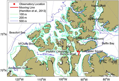
A real-time ocean observatory was installed and has been operational since August 2011 off Gascoyne Inlet on the south coast of Devon Island in the eastern Northwest Passage (Fig. 1). It is just 30 km west of the location where the decade-long time series of instrumented mooring observations were made. The observatory cable was extended in the summer of 2012 to a depth of 165 m, 2.25 km south of the open coast. The project was initiated to provide real-time ice and ocean data for use by mariners and for input to sea-ice forecasting and climate models. The ice–ocean connections identified from the long time series mooring data now present the opportunity to use the real-time data as an ice-forecasting tool.

Fig. 1 Location of the Barrow Strait Ocean Observatory at the eastern end of the Northwest Passage, the principal transportation corridor through the Canadian High Arctic. Analyses of data from a long-term monitoring array just to the east (also shown), identified a link between water salinity and the timing of freeze-up (Hamilton et al. (2013)) that allows the real-time observatory data to be used to forecast freeze-up.

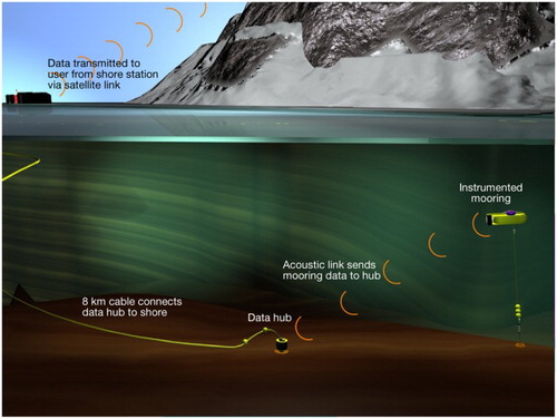
The observatory (Fig. 2) consists of three components: an acoustic telemetry link that passes data from instruments on a sub-surface mooring (the node) to an underwater hub, an 8 km long sub-sea cable that carries data from the hub to a shore station located in the inner reaches of Gascoyne Inlet, and a two-way satellite link that transmits the data from the shore station to the user. Because it is vulnerable to ice damage, the cable passes through a buried pipe at the beach to protect it.

Fig. 2 An illustration of the observatory in eastern Barrow Strait. Data are transmitted acoustically from an instrumented mooring to a data hub at the end of an 8 km long sub-sea cable, then through the cable to a shore station for transmission via a two-way Iridium satellite link.

Instrumentation on the node mooring consists of a Sea-Bird SBE37 to provide the required salinity and temperature information and an RDI 307 kHz ADCP with companion pole compass (Hamilton, 2001) to measure currents, as well as the presence and velocity of sea ice. The ADCP also records acoustic backscatter, which can be interpreted to obtain a zooplankton biomass index (Hamilton et al., 2013). These instruments are configured for bihourly sampling (that is, once every two hours), and their data streams are output to a dual port Teledyne Benthos acoustic modem. The acoustic modem logs all incoming data internally until it is interrogated for data offload by a second acoustic modem mounted in the hub mooring, which is controlled by a custom hub controller and electronics package. At the end of a sampling period, the hub controller interrogates the node acoustic modem to retrieve the latest dataset and store it locally. The hub controller then signals the shore station via the sub-sea cable that new data are available, which prompts the autonomous shore station controller to “talk” with the hub controller to get system status, modify any settings, and offload the data files. Low power cable modems make data transmission over the 8 km cable possible. In order to conserve battery power, when the shore station completes interrogation of the hub it instructs the hub controller to return to a very low power sleep mode until the next sample time. The shore station then samples an onboard barometer and an onboard GPS which it uses to get an accurate time and correct for any clock drift in the system.

The shore station controller establishes an Iridium Router-Based Unrestricted Digital Internetworking Connectivity Solutions (RUDICS) connection to a server based at the Bedford Institute of Oceanography. This server runs custom software that automatically handles incoming data transmissions and data archiving, providing the user with an interface for control and reconfiguration of the remote system. After the connection has been established, the remote server interrogates the Arctic-based shore station, downloading the data, executing any commands requested by the user, and instructing the shore station to return to its low power sleep mode. The entire Iridium session usually takes about two minutes.

3 Freeze-up forecasts for 2012 and 2013

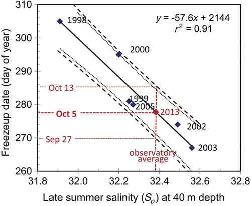
Continuous bihourly observatory salinity measurements from 40 m depth have provided the data required to make freeze-up predictions for each of the last two years using the relationship between freeze-up date and late summer (5 August–21 September) salinity identified by Hamilton et al. (2013) and shown in Fig. 3. The superimposed observatory-based average late summer salinity for the 40 m level in 2013 provides a freeze-up prediction of 5 October with 80% confidence limits of ±7.9 days. Here, following Draper and Smith (1966), the confidence bounds are the ones within which 80% of future individual observations are expected to lie. (The bounds shown in Hamilton et al. (2013) are for the true mean value of freeze-up date for a given salinity value.)

Fig. 3 The observed relationship between freeze-up date and late summer 40 m salinity in northern Barrow Strait, with an observatory-based prediction for the 2013 freeze-up shown in red. The late summer (5 August–21 September) salinity average for 2013 was computed from observatory measurements and provides a predicted freeze-up date centred on 5 October (day 278), with 80% confidence of occurrence (the dashed lines) between 27 September and 13 October. The lighter dotted lines show the 80% confidence limits when the 2013 data point is included in the regression.

The accuracy of the 2013 forecast is shown in Fig. 4. Here the observed freeze-up is based on CIS daily ice charts (http://www.ec.gc.ca/glaces-ice/), with freeze-up being defined as the first date when ice cover at the mooring site is 9/10 or more (the combined fractional surface area of all types of ice is greater than 90%, with less than 10% being open water or open leads) for two days in a row. Hamilton et al. (2013) defined freeze-up as the first time in autumn that the ADCP they used as an ice-cover indicator returned 10 consecutive bihourly ice velocity measurements. ADCP data were not available in 2012 and 2013 because of a technical issue that caused the instrument battery to deplete within a week. But freeze-up date determined from the ice charts can be compared with the date determined from the ADCP ice-tracking feature over the seven years (1999–2005) for which we have data from both sources at this location. Rejecting the datum from one year when there was a 13-day difference for an unknown reason, the freeze-up date determined from the CIS ice charts occurred two days earlier, on average, than that provided by the ADCPs, with the standard deviation of the difference between the two methods being ±1.9 days.

Fig. 4 Freeze-up forecast accuracy in eastern Barrow Strait for 2013. The prediction is shown as the red bar centred on 5 October, bracketed by the period during which there is 80% confidence that freeze-up will occur. The histogram shows daily best estimates of ice concentration from CIS ice charts that are based on data from a variety of sources (satellite imagery and ship and aircraft-based visual observations).

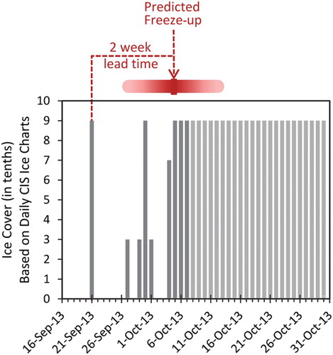
The forecast timing of freeze-up agrees well with observations. The ice charts demonstrate that freeze-up was twice preceded by the formation and disappearance of new ice, with near-full (9+/10) ice cover forming on 5 October and persisting thereafter. The lightened grey bars in Fig. 4 after 7 October indicate a presumption of complete or near-complete ice cover because no CIS analysis was available for the specific observatory area after that date because by then the ice edge had progressed well to the east with 9/10 and 9+/10 coverage indicated for all but the easternmost part of Lancaster Sound.

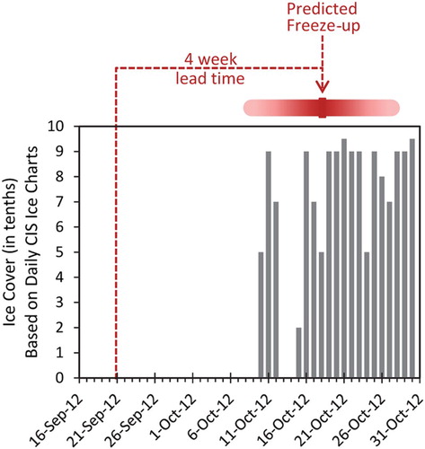
A similar freeze-up forecast was made for 2012 (Fig. 5). Here a shortened late summer averaging period was used (4 to 21 September rather than 5 August to 21 September) to derive a modified freeze-up versus late summer salinity regression (not shown). This was required because the extension of the observatory cable (mentioned previously) was not completed until 4 September. Observatory data prior to that were considered to be too close to the coast to be representative of the broader northern Barrow Strait area. With the shorter averaging period, the regression has a lower coefficient of determination (r² = 0.85) and wider confidence limits but is still useful for providing a freeze-up forecast. The resulting forecast for freeze-up was 18 October with 80% confidence of occurrence between 8 and 28 October. Actual freeze-up, based on daily CIS ice charts, occurred on 19 October, which is two weeks later than in 2013. The forecast once again closely matched the timing of the observed freeze-up and provided four weeks’ advance notice for 2012.

Fig. 5 Freeze-up forecast accuracy in eastern Barrow Strait for 2012. The prediction, made four weeks in advance of observed freeze-up, is shown as the red bar centred on 18 October, bracketed by the period during which there is 80% confidence freeze-up will occur. The histogram shows daily best estimates of ice concentration from CIS ice charts.

4 Discussion

The results demonstrate a new capability for accurate prediction of freeze-up in northern Barrow Strait. Because the forecast is based on a late summer salinity average that requires observatory measurements up to 21 September, and observed freeze-up there ranges from late September to early November, the forecast lead time is from 4 days to 6 weeks. To increase the forecast lead time, our analysis indicates that a reliable prediction is possible if the end of the late summer averaging period is shortened by one week. However, shortening the averaging period further results in a rapid deterioration in the strength of the regression. This appears to be a result of excluding data during a rapid decrease in salinity in the first half of September that is seen in many years.

The potential for a general indicator of the timing of freeze-up months in advance of its occurrence is suggested by a moderately strong relationship between freeze-up and early summer (21 June to 5 August) temperature averaged over the water column (Hamilton et al., 2013). The observatory presently only provides real-time temperature data from 40 m depth, so using this relationship as an early predictor of freeze-up is not currently feasible. Further expansion of the observatory to include real-time temperature measurements from 80 and 150 m will make that possible. Until then, internally recorded conductivity-temperature-depth (CTD) measurements at those levels are being collected, which will allow us to add data points to that regression, thereby improving confidence in this freeze-up versus early summer water column temperature relationship.

The impact of adding data to the regressions used for forecasting is illustrated by including the 2013 data point in the statistical calculations describing the least squares fit to the data in Fig. 3. Although the slope and coefficient of determination do not change, the 80% confidence limits are reduced by 15% (the dotted lines in Fig. 3), from ±7.9 days to ±6.7 days, at our 2013 salinity observatory value. Additional data have the potential to further reduce the confidence limits in Fig. 3, but because approximately 9% of the variability in the timing of freeze-up is unrelated to salinity (r² = 0.91), other factors (such as weather) play some role. Given that the date of freeze-up varies by about 40 days in this area, the unaccounted for variability sets a lower limit, of about ±2 days, on how tightly the freeze-up prediction can be constrained.

Practical forecasting of break-up at this location may also be possible with real-time measurements. Hamilton et al. (2013) show that break-up is very strongly negatively correlated to mid-spring water temperature at 40 m, that is, break-up is earlier in years when the water is warmer in mid-spring. They defined break-up as the first time in the year when ice-tracking ADCPs do not return an ice velocity measurement for 10 consecutive samples (a 20-hour period). In two of the years for which they had data, this definition identified break-up anomalously early. But in those years the cover remained broken for just a few days. The ADCPs indicated that there was a return to 100% coverage thereafter, which remained for several more weeks. This behaviour points to the issue of the definition of terms. Definitions, and which observations are relevant, may vary depending on the user (Eicken, 2013). For maritime operations, an anomalous, short-duration, local occurrence of broken ice is not important. The time when the passage becomes navigable for the summer season is more relevant. Future work will compare ADCP-based break-up timing with archived ice charts to establish an objective and relevant definition for break-up so that the break-up forecasting capability of the observatory can be tested.

Other future work includes adding ice draft data to the observatory data stream. Real-time ice draft information is of direct use to mariners and as input to ice-forecasting models. It may also provide improved capability for forecasting ice break-up because early break-up is linked to warmer spring water temperature, presumably because the additional heat erodes the ice from below.

The close relationship between late summer 40 m salinity and the timing of freeze-up observed on the north side of eastern Barrow Strait allows for local freeze-up forecasts. We cannot assume the same relationship holds in other locations, although in areas where physical processes are similar (e.g., mean flows are low and upper ocean salinity reflects mixed-layer depth), it may be the case. Regardless, the results presented here demonstrate the value of data from long time series in providing a means of exploring relationships between key physical variables on interannual time scales, thereby shedding light on local physical processes and potentially providing predictive capability when coupled with real-time measurements.

Without historical data, real-time ice and ocean information are still valuable, particularly when provided from strategic locations where they can be used by marine operators and planners to improve the safety and efficiency of marine operations. These real-time data are also valuable for validating and improving ice forecast models, and with time they also provide long time series that may offer future predictive capability. The prototype observatory described here is a replicable new technology that provides a means of acquiring real-time ice and ocean data at strategic locations. Although the instrument interface and communications control electronics and software are custom designed, the oceanographic instrumentation and acoustic, cable, and satellite modem technology used are commercially available. Potential sites require some natural protection from onshore rafting of ice where the cable comes ashore and reasonable accessibility by ship for servicing. The biggest logistical challenge is the installation of a protective pipe through the beach that serves to protect the cable at this vulnerable location. Further offshore, damage of the sub-sea cable by iceberg scour is the biggest risk to the deployed system, but this risk may be at least partially mitigated by site and/or cable route selection. Servicing of the observatory is required annually and consists of replacement of the node moorings and the cable hub, as well as recharging of shore station batteries.

5 Conclusions

Interest in real-time ocean observatories is growing as these installations become more technically and economically feasible. Real-time data can provide a valuable description of local conditions for use by marine operators and valuable input to forecast models for both seeding and validation of these models. But the combination of real-time data and prior knowledge derived from long-term monitoring can also provide a useful forecasting tool. This has been demonstrated here by using real-time salinity measurements and a previously established salinity–freeze-up relationship to accurately forecast local freeze-up timing with a lead time of two to four weeks. As future observatory sites are chosen and systems are developed, it is useful to consider appropriate monitoring by traditional means to start building time series that have the potential to greatly enhance the value of the observatory once in place.

Acknowledgements

We thank Defense Research and Development Canada (DRDC-Atlantic) who contributed to the development of this observatory by sharing facilities and providing logistical support at their Northern Watch site on Devon Island. Thanks also go to the Canadian Coast Guard for their valuable ship and logistical support. We also thank the anonymous reviewers for their useful comments and suggestions, as well as our internal reviewers, Dave Hebert and Simon Prinsenberg. Funding for the development of the observatory was provided by the Canadian Department of Fisheries and Oceans (Maritime Region, the National Centre for Arctic Aquatic Research Excellence (NCAARE), the Aquatic Climate Change Adaptation Services Program (ACCASP), the Program of Energy Research and Development (PERD, Natural Resources Canada), and the Canadian Operational Network of Coupled Environmental Prediction Systems (CONCEPTS).

References

- Draper, N. R., & Smith, H. (1966). Applied regression analysis. New York, NY: John Wiley & Sons.
- Drobot, S. D., & Maslanik, J. A. (2002). A practical method for long-range forecasting of ice severity in the Beaufort Sea. Geophysical Research Letters, 29(8), 1213. doi:10.1029/2001GL014173
- Eicken, H. (2013). Arctic sea ice needs better forecasts. Nature, 497, 431–433. doi: 10.1038/497431a
- Hamilton, J. M. (2001). Accurate ocean current direction measurements near the magnetic poles. In Proceedings of the 11th International Offshore and Polar Engineering Conference ISOPE (Vol. 1, pp. 656–660). Stavanger, Norway.
- Hamilton, J. M., Collins, K., & Prinsenberg, S. J. (2013). Links between ocean properties, ice cover, and plankton dynamics on interannual time scales in the Canadian Arctic Archipelago. Journal of Geophysical Research: Oceans, 118, 5625–5639. doi:10.1002/jgrc.20382
- Hamilton, J. M., & Wu, Y. (2013). Synopsis and trends in the physical environment of Baffin Bay and Davis Strait (Can. Tech. Rep. Hydrogr. Ocean Sci. Report No. 282).
- Holland, M. M., & Stroeve, J. (2011). Changing seasonal sea ice predictor relationships in a changing Arctic climate. Geophysical Research Letters, 38(18), 1–6. doi:10.1029/2011GL049303
- Howell, S. E. L., Duguay, C. R., & Markus, T. (2009). Sea ice conditions and melt season duration variability within the Canadian Arctic Archipelago: 1979–2008. Geophysical Research Letters, 36, L10502. doi:10.1029/2009GL037681
- Hu, X., & Myers, P. G. (2014). Changes to the Canadian Arctic Archipelago sea ice and freshwater fluxes in the twenty-first century under the Intergovernmental Panel on Climate Change A1B Climate Scenario. Atmosphere-Ocean, 52(4), 331–350. doi:10.1080/07055900.2014.942592
- Lindsay, R. W., Zhang, J., Schweiger, A. J., & Steele, M. A. (2008). Seasonal predictions of ice extent in the Arctic Ocean. Journal of Geophysical Research: Oceans, 113(C2), 1–11. doi:10.1029/2007JC004259
- Petrich, C., Eicken, H., Zhang, J., Kreiger, J., Fukamachi, Y., & Ohshima, K. I. (2012). Coastal landfast sea ice decay and breakup in northern Alaska: Key processes and seasonal prediction. Journal of Geophysical Research: Oceans, 117, C02003. doi:10.1029/2011JC007339
- Sigmond, M., Fyfe, J. C., Flato, G. M., Kharin, V. V., & Merryfield, W. J. (2013). Seasonal forecast skill of Arctic sea ice area in a dynamical forecast system. Geophysical Research Letters, 40, 529–534. doi:10.1002/grl.50129
- Stroeve, J. C., Kattsov, V., Barrett, A., Serreze, M., Pavlova, T., Holland, M., & Meier, W. N. (2012). Trends in Arctic sea ice extent from CMIP5, CMIP3 and observations. Geophysical Research Letters, 39, L16502. doi:10.1029/2012GL052676
- Tivy, A., Alt, B., Howell, S., Wilson, K., & Yackel, J. (2007). Long-range prediction of the shipping season in Hudson Bay: A statistical approach. Weather and Forecasting, 22(5), 1063–1075. doi: 10.1175/WAF1038.1
- Tivy, A., Howell, S. E. L., Alt, B., McCourt, S., Chagnon, R., Crocker, G., … Yackel, J. J. (2011). Trends and variability in summer sea ice cover in the Canadian Arctic based on the Canadian Ice Service digital archive, 1960–2008 and 1968–2008. Journal of Geophysical Research: Oceans, 116, C03007. doi:10.1029/2009JC005855