Identifying the Origin of Anomalous High Tropospheric Ozone in the Ozonesonde Data at Uccle by Comparison with Nearby De Bilt

Abstract

The ozonesonde stations at Uccle (Belgium) and De Bilt (Netherlands), separated by only 175 km, offer a unique opportunity to test the influence of different ozonesonde types and different correction strategies, as well as to detect the presence of inhomogeneities in the ozonesonde time series resulting from changes in sounding equipment (solution, radiosonde, ozonesonde, interface, sounding software, etc.). In particular, we highlight a 2.5 year period (beginning of 2007 to mid-2009) of anomalous high tropospheric ozone values measured by ozonesondes at Uccle and compare these with the observations from De Bilt. Because the ozone deviations are only observed in the free troposphere where ozone concentrations are relatively low, and not in the boundary layer or the stratosphere, this issue is directly related to the sensitivity of ozonesondes. Therefore, the effect of every instrumental change, even though small, during this 2.5 year anomalous period is analyzed considering a change in the radiosounding equipment, different ozonesonde batches, operational differences at the stations, differences on ascent and descent during the anomalous period; an environmental cause is also examined. Unfortunately, one single, specific cause for the observed high tropospheric ozone values at Uccle could not be identified. There are two explanations consistent with the observations and not ruled out by the analysis here: 1) the majority of the ozonesondes used at Uccle between March 2007 and August 2009 needed longer conditioning of their sensors and, therefore, behaved more accurately at low ozone concentrations during their descent or when used a second time, and 2) an environmental origin arising from a local difference in the air mass between Uccle and De Bilt and between the ascent and descent.

Résumé

[Traduit par la rédaction] Les stations de sondage d'ozone d'Uccle (en Belgique) et de De Bilt (aux Pays-Bas), séparées de seulement 175 km, fournissent une occasion unique de vérifier l'influence de différents types de sondes d'ozone et de différentes stratégies de correction ainsi que de détecter la présence d’éléments non homogènes dans les séries chronologiques des sondes d'ozones découlant de changements dans l’équipement de sondage (solution, radiosonde, sonde d'ozone, interface, logiciel de sondage, etc.). En particulier, nous distinguons une période de 2,5 ans (du début de 2007 au milieu de 2009) de valeurs anormales d'ozone dans la haute troposphère mesurées par des sondes d'ozone à Uccle et nous comparons ces valeurs aux observations de De Bilt. Étant donné que les écarts d'ozone ne sont observés que dans la troposphère libre où les concentrations d'ozone sont minimales, et non pas dans la couche limite ou dans la stratosphère, cette question est directement liée à la sensibilité des sondes d'ozone. Par conséquent, l'effet de chaque changement instrumental, même petit, durant cette période anormale de 2,5 ans est analysé en fonction d'un changement dans l’équipement de radiosondage, de différents lots de sondes d'ozone, de différences opérationnelles aux stations ou de différences lors de la montée et de la descente durant la période anormale; nous examinons aussi la possibilité d'une origine environnementale. Malheureusement, nous n'avons pas pu identifier une cause unique pour les valeurs d'ozone observées dans la haute troposphère à Uccle. Il y a deux explications en accord avec les observations que l'analyse n'a pas pu rejeter : 1) la majorité des sondes d'ozone utilisées à Uccle entre mars 2007 et août 2009 avaient besoin d'une plus longue période d'acclimatation pour leurs capteurs et donc fonctionnaient mieux par faibles concentrations d'ozone durant leur descente ou lorsque utilisées une deuxième fois et 2) une origine environnementale découlant d'une différence locale dans la masse d'air entre Uccle et De Bilt et entre la montée et la descente.

Keywords:

• ozone
• troposphere
• ozonesonde
• instrument comparison
• data quality assessment

1 Introduction

Although only a minor constituent in the Earth's atmosphere, ozone plays an important role in the physics and photochemistry of the atmosphere. Ozone absorbs both infrared and ultraviolet radiation and, therefore, acts as both a greenhouse gas and an ultraviolet (UV) filter for the Earth's biota. Ozone is a strong greenhouse gas, particularly in the region of the tropopause whereas ozone molecules residing in the stratospheric ozone layer, between 20 and 25 km, protect us from harmful solar UV radiation. In the past, the focus has been on the stratospheric ozone layer, because its density decreased substantially as a result of anthropogenic emissions of ozone-depleting substances (ODSs) (with chlorofluorocarbons being the typical example). Thanks to regulation of these ODSs by the 1987 Montreal Protocol, stratospheric ozone concentrations will recover over the next decades (Newman et al., 2009; WMO, 2011). However, tropospheric ozone (including boundary layer ozone) has deleterious effects on human health and vegetation (Logan et al., 2012). Regional air quality has degraded in urban areas during the last few decades by, for example, increasing concentrations of tropospheric ozone as a result of increasing emissions of nitrogen oxides (NO_x), methane, carbon monoxide, and hydrocarbons.

Because ozone photochemistry and, therefore, the effects of ozone on human health depends strongly on atmospheric conditions and, hence, on the location of the ozone molecules in the atmosphere, knowledge of the vertical distribution of ozone is of crucial importance. For more than half a century, ozonesondes attached to weather balloons have provided these data at very high vertical resolution (typically a few 100 m), up to altitudes in the range of 30 to 35 km. Ozonesondes constitute the most important data source for deriving long-term ozone trends with sufficient vertical resolution up to about 20 km but have also been widely used to study photochemical and dynamical processes in the atmosphere and to validate and evaluate satellite observations and their long-term stability (Smit et al., 2011). A major concern for any research using ozonesonde measurements is the homogeneity and consistency of the data because every ozonesonde is a unique instrument and different types of ozonesondes exist. Consequently, every ozonesonde needs to be calibrated thoroughly prior to launch. To have consistency between different ozonesonde stations, it is essential to have agreement on the preparation procedures as well as agreement on the procedures for data processing and analysis (Smit et al., 2011).

The ozonesondes studied in this paper are Electrochemical Concentration Cell (ECC) ozonesondes, which were developed by W. Komhyr (Komhyr, 1969; Komhyr & Harris, 1971). The ECC ozone sensor consists of two half cells, made of Teflon, linked together by an ion bridge and containing different concentrations of a potassium iodide (KI) solution, thereby serving as cathode and anode chambers. A miniature piston pump in the same chemically inert material (Teflon) takes air into the cathode chamber at a constant rate. During operation, the ozonesonde is put in a styrofoam isolating box, and the pump ingests the ambient air outside the box into the cathode. The ozone molecules present in the ambient air will then interact with the KI solution in the cathode chamber, leading to a net release of two electrons per ozone molecule. Hence, the electric current generated can be related directly to the uptake rate of ozone in the cathode chamber and then to the amount of ozone molecules in the atmosphere (ozone partial pressure (mPa)), if additionally the pump flow rate Φ_p (cm³ s⁻¹) and the pump temperature T_p (K) are known (Smit et al., 2011):(1)

The electric cell current I_M (µA) and the pump temperature are measured during the flight and are transferred via an electronic interface from the ozonesonde to a meteorological radiosonde on the same balloon. The radiosonde transmits those measurements, together with the temperature, pressure, humidity, and wind direction and speed, to the ground receiving station. The pump flow rate Φ_p is measured in the laboratory before launch by recording the time needed to pump 100 cm³ of ambient air through the solution. Also, the background current I_B (μA) is measured prior to launch and represents the current generated by the ozone sensor when sampling ozone-free purified air. Finally, the conversion efficiency η_c is determined by the absorption efficiency of O₃ into the sensing solution and the stoichiometry of the O₃ conversion. During normal operation the conversion efficiency is about one at neutral pH and usually a buffer is added to the cathode KI solution to keep it neutral and another is added to stabilize the O₃ conversion (Smit et al., 2011). Post-flight data processing is needed to account for the decrease in the pump flow efficiency at low pressures compared with the pump performance under laboratory conditions. Different correction tables exist, and all are based on empirical averages obtained from pump flow efficiency measurements made at different air pressures in a vacuum chamber. Provided that the measured ozonesonde profiles were normalized to ground-based total ozone column measurements at the launch site, the precision of various ozonesonde types in the stratosphere up to about 28 km is within ±3%, while any systematic biases compared with other ozone-sensing techniques are smaller than ±5%. In the troposphere, where ozone concentrations are lower than in the stratosphere, the impact of instrumental errors and variability is larger (Smit et al., 2011). The same World Meteorological Organization/Global Atmospheric Watch (WMO/GAW) report concludes that ECC ozonesondes have a precision of 3 to 5% and an absolute accuracy of about 10% in the troposphere, because different sonde manufacturers and preparation techniques introduce tropospheric biases of ±5%.

In this paper, we report on the detection of anomalous high tropospheric ozone concentrations in the Uccle ozonesonde time series between the beginning of 2007 and mid-2009. To attribute probable causes for this anomalous tropospheric ozone behaviour, we compare the data from Uccle with the ozonesonde data from the nearby station at De Bilt, in the Netherlands. However, it should be noted that these stations use different ozonesonde types, different operating procedures, and different correction algorithms are applied to the raw data. Therefore, in the first section, we will describe the characteristics of the ozonesonde datasets acquired at both stations. In Section 3, the ozone anomaly event in the Uccle data is presented, followed by the investigation of the causes in Sections 4 and 5. Finally, in Section 6, we present the conclusions.

2 Data

The Uccle ozonesonde station (50°48′ N, 4°21′ E, 100 m above sea level (asl)) is located in the southern residential area of Brussels (approximately 1 million inhabitants), the capital of Belgium. It is classified as a suburban station, according to European standards (European Union, 2008). Since January 1969, ozonesonde launches have been carried out three times weekly (Monday, Wednesday, and Friday), with only some minor interruptions. In April 1997, the switch from the Brewer-Mast to the Model-Z Enviromental Science Corporation (ENSCI) ECC ozonesonde was made (De Backer, De Muer, & De Sadelaer, 1998) and the same model type (although produced by another company since 2010) is still in use. In this paper, we will focus on the ECC ozonesonde measurements in Uccle in particular, which, apart from ozonesonde batch differences, form a homogeneous dataset, because the manufacturer's recommended cathode sensing solution strength (SST) of 0.5% KI has been used consistently. An overview of the ozonesonde properties is also given in Table 1.

Table 1. Overview of the properties of the ozonesonde measurements at Uccle and De Bilt.

	Uccle	De Bilt
Coordinates	50°48′ N, 4°21′ E, 100 m asl	52°10′ N, 5°18′ E, 4 m asl
First launch	January 1969	November 1992
Average frequency	3/week	1/week
Sonde types	Brewer-Mast	Science Pump ECC 5A
(switch date)	ENSCI ECC 6Z	Science Pump ECC 6A
	(1 April 1997)	(24 July 1997)
RS types for ECC	RS80	RS80
(switch date)	RS92	RS92
	(September 2007)	(November 2005)
ECC SST	0.5	1.0
Solution amount	3.0 cc	2.5 cc
		3.0 cc (from 23 November 1994)
Location of Tp sensor	In the pump	In the box
		In the pump (from 5 November 1998)
IB measurement	In laboratory before exposure to O3	At launch site after exposure to O3
IB subtraction	Constant	Constant
Total O3 normalization	Yes, pressure-dependent	No
Φp efficiency correction	In-house (see text)	Manufacturer's correction table

The ozonesonde station at De Bilt (52°10′ N, 5°18′ E, 4 m asl) lies to the east of Utrecht (about 300,000 inhabitants), and about 50 km to the south of Amsterdam, the capital of the Netherlands. The ozonesonde program started at the end of November 1992 and a total of more than 1000 launches has been carried out; so, on average, there is one launch every week. The ECC ozonesonde used is manufactured by Science Pump, but two different types were used during the period of record: the Science Pump 5A and 6A (since 24 July 1997). The cathode cells have always been filled with the recommended solution strength of 1% KI, but the amount changed from 2.5 to 3.0 cc on 23 November 1994. There are other differences in the operating procedures at the Uccle and De Bilt stations (see Table 1): a different measurement of the background current (measured before exposure to ozone at Uccle and after exposure to ozone at De Bilt), and the fact that the temperature measurement through an orifice in the pump only started in De Bilt on 5 November 1998 (before this date, the temperature sensor was located “somewhere” in the styrofoam box).

Both stations also apply different correction algorithms to the retrieved vertical ozone profile data. At De Bilt, the standard correction algorithms are applied (i.e., the pump flow correction table provided by the manufacturer, no normalization to the total ozone column, and a constant background current subtraction (certainly after 5 November 1998)). At Uccle, an alternative method for correcting the ozone profiles for decreasing pump efficiency with altitude was developed (De Backer et al., 1998; De Backer, 1999). First, the change in the pump efficiency with decreasing temperature is additionally corrected for. Second, the correction for the decrease in pump efficiency with decreasing pressure is applied simultaneously with the normalization to the total ozone column, using a pressure-dependent correction factor parameterized to match (i) the single point calibration of the ozone sensor at the laboratory (the so-called “calibration factor” obtained by applying ozone-containing air, at about 320 µg m⁻³, from a calibrated ozone source to the operating sensor for 10 minutes), and (ii) the total ozone measured with a spectrophotometer at the same site. The same method is applied to both the Brewer-Mast and ECC ozonesondes, constructing a homogeneous data series with ozone differences within 2% over almost the entire altitude range (De Backer et al., 1998; Lemoine & De Backer, 2001).

3 Anomalous high tropospheric ozone at Uccle

Logan et al. (2012), in a paper describing tropospheric ozone changes over Europe based on an analysis of ozone measurements from sondes, regular aircraft (Measurement of Ozone and Water Vapor aboard Airbus In-service Aircraft (MOZAIC)), and alpine surface sites, pointed to anomalous behaviour in the Uccle ozonesonde data record during the 2007–09 period. In the paper, the time series of the profile datasets of different European stations are compared for the average of two levels in the lower troposphere (681 and 584 hPa or 2.6 to 5 km) and the middle troposphere (500 and 430 hPa or 5 to 7.2 km). For those layers, the authors found that “the mean bias between Uccle and the other two long-term stations (Payerne and Hohenpeißenberg) is small between 1993 and 2006, less than 3.5 ppb, with σ ≈ 4.0 ppb. Ozone is higher at Uccle from 2007 to 2009 than at the other two stations by about 5 to 20 ppb, with mean biases of 7 to 10 ppb (see Logan et al., 2012, their Table 2), and it is also higher than measured at De Bilt which is only 155 km away, suggesting a problem with the data from this altitude range during those years.” Furthermore, the authors describe the monthly MOZAIC time series as coherent because of the similarity of the time evolution at the various locations and the small mean biases between locations and, therefore, compared the same layers of ozonesonde data with a combined Frankfurt/Munich time series. From the same Table 2, it can be seen that the mean biases and standard deviations between the Uccle ozonesonde set and this combined MOZAIC data are in the same range from 2007 to 2008 for those specific layers. These values are significantly higher than for the comparison of the earlier Uccle ECC ozonesonde data record (1997–2006) and are also higher than the values found for the MOZAIC–ozonesonde comparisons for the other two stations. Moreover, a direct comparison of the MOZAIC mid-tropospheric and Upper Troposphere, Lower Stratosphere (UTLS) ozone measurements above Brussels with the Uccle sonde data, based on back trajectories, confirmed these discrepancies during the same period (Staufer et al., 2013).

Table 2. Statistical properties (mean, standard deviation, and number) of the deviations in integrated ozone amounts in the 3–8 km layer for quasi-simultaneous observations at Uccle and De Bilt (see also Fig. 1d), calculated for different batches of ENSCI model Z ECC ozonesondes and different periods. The “bad period” is defined to be from 1 March 2007 (start of use of Z10… ozonesondes) to 1 August 2009 (start of use of Z13… or Z14… ozonesondes); the good period is then outside this period.

(a)	Mean	SD	n
Overall	0.33	12.10	1424
Good period	−0.02	9.55	1196
Bad period	2.16	21.55	228
Z < 10 …	−0.04	9.34	941
Z = 10 …	2.44	24.38	99
Z = 11 …	1.33	15.31	107
Z = 12 …	2.11	15.76	82
Z = 13 …	−0.27	7.01	51
10 … ≤ Z ≤ 12 …	1.93	18.66	288
Z > 13	−0.23	11.09	195
	Good Period			Bad Period
(b)	Mean	SD	n	Mean	SD	n
Z < 10 …	−0.04	9.35	933	−0.58	7.89	8
Z = 10 …	0.94	3.85	8	2.57	26.04	91
Z = 11 …	1.04	9.50	23	1.40	17.01	84
Z = 12 …	0.72	6.71	37	3.24	20.60	45
10 … ≤ Z ≤ 12 …	0.86	7.15	68	2.26	21.80	220

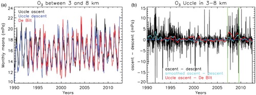
In this paper, to identify and characterize the anomalous ozone behaviour in the Uccle ozonesonde record in more detail, we compare the Uccle data directly with the nearby De Bilt ozonesonde data for different atmospheric layers. In Figs. 1a, 1b, and 1c, respectively, the monthly time series for the two stations are shown for the integrated total ozone in (i) the boundary layer (h < 3 km), (ii) the free tropospheric layers between 3 and 8 km, and (iii) the stratosphere (h larger than the tropopause height, which is on average around 11 km at Uccle and De Bilt). It should be noted that, although different ozonesonde types are used, and different correction strategies are applied, the Uccle and De Bilt ozonesonde time series are very similar. The larger variability in the De Bilt monthly mean time series can be ascribed to the lower frequency of ozonesonde launches. However, from Fig. 1b, it should also be obvious that, during a 2.5-year period (from the beginning of 2007 to mid-2009), the Uccle station consistently measures higher free tropospheric ozone values than at the nearby De Bilt station, but not in the boundary layer (Fig. 1a) or in the stratosphere (Fig. 1c). Moreover, comparison of the ozonesonde data with the output of a chemical transport model (Chemistry transport model maintained by the Laboratory of Dynamic Meteorology at the École Polytechnique, France (CHIMERE)) showed good agreement at the boundary layer for the 1990–2010 time period (Decloo, Van Malderen, & De Backer, personal communication, 2011). At a polluted site such as Uccle, boundary layer ozone concentrations are usually higher than the free tropospheric ozone amounts. Hence, the anomalous behaviour seen in the Uccle ozonesonde data arises only at levels where ozone concentration is low.

Fig. 1 Monthly mean comparison plots between integrated ozone amounts for the Uccle (black) and De Bilt (red) ozonesonde stations for different parts of the atmosphere: (a) boundary layer (0–3 km), (b) free troposphere (3–8 km), and (c) stratosphere (h > tropopause height). In (d), the deviations in integrated ozone amounts in the 3–8 km layer are shown, in black, for quasi-simultaneous (dt < 1.5 day) observations at Uccle and De Bilt. The red curve represents a boxcar average of these deviations with width equal to 50 days; the green vertical lines denote the breakpoints in the mean of the time series found by a statistical test.

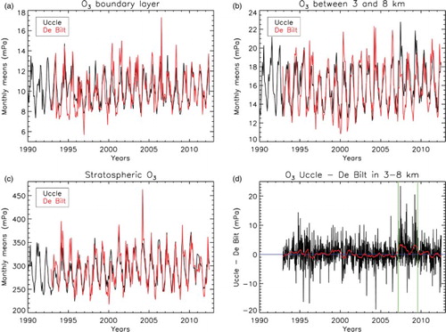
A more detailed look at the differences in tropospheric ozone measured at Uccle and De Bilt is provided in Fig. 1d. Here, we calculated the differences in the amounts of integrated total ozone in the layers between 3 and 8 km for quasi-simultaneous (i.e., a launch time difference of at most 1.5 days) ozone soundings at Uccle and De Bilt. By not comparing monthly data, but rather comparing quasi-simultaneous data, we can directly link the differences to individual Uccle ozonesondes and their properties. Because the stations are located close to one another, both stations have agreed to launch preferentially on different days, so that only a small number of simultaneous ozone soundings exist, and we must restrict ourselves to quasi-simultaneous launches for this detailed analysis. Nevertheless, the differences in tropospheric ozone between both stations are quite constant in time, but the anomalous high ozone values at Uccle in the 2007–09 period stand out. Statistical tests used to identify a stepwise shift in the mean of the time series (e.g., see Van Malderen & De Backer, 2010 and references therein) detected the beginning and end of the anomalous period as statistically significant change points and identified these dates as mid-February 2007 and the beginning of August 2009, respectively. These dates are denoted by vertical green lines in the figure.

4 Instrumental causes

Clearly, there is an issue in the Uccle ozonesonde data in February/March 2007 to August 2009. However, during this period, the ozonesonde operators maintained the same procedures for pre-flight preparation and calibration of the ozonesondes and also used the same correction algorithms for post-processing of the data. There were only three instrumental changes during this period:

• The Vaisala radiosounding equipment was changed in the summer of 2007, when we replaced the LOng RAnge Navigation (LORAN-C) system with a Global Positioning System to be able to track the RS92 radiosondes instead of the older RS80 type. With this new system, the data transmission is digital, and a new interface is required to connect the ozonesonde to the RS92 radiosonde. Vaisala also provides software for the data processing, incorporating the standard correction algorithms. The first flight with the new system occurred on 23 May 2007; during the following three months, we alternated between the two systems and some double radiosonde launches were carried out. From September 2007 onwards, only the new system and equipment were used.

• There was an update of the sounding software in November 2009 that should have affected only the temperature measurements. The next software update, affecting the temperature and humidity measurements, was installed in June 2011.

• There was an annual change in the batches of ECC ozonesondes.

In this section, we will now investigate whether or not these instrumental changes might explain the high tropospheric ozone values measured at Uccle during the 2007–09 period.

a Radiosounding Equipment Change

At Uccle, the ozone profile data are calculated from the raw data (electric currents) instead of using the sounding software. This is necessary, because in some versions of the sounding software, errors in the background current subtraction are present (a pressure-dependent background current subtraction was used for the ENSCI ECC ozonesondes in the Vaisala MW31 software, versions 3.52 to 3.62, Vaisala personal communication, 2011). For the meteorological variables, we used the state-of-the-art software provided by Vaisala, but we re-simulated all historical RS92 launches, so that these variables would be reprocessed by the same algorithms and scripts. So, the software update that took place in November 2009 cannot be responsible for marking the end of the period of anomalous behaviour. Because the reprocessing of the ozone data from the raw data uses the same algorithms before and after the radiosounding equipment change in mid-2007, the operational software has no direct effect on the retrieved ozone values.

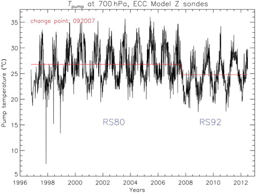
As can be seen in Fig. 2, the radiosounding equipment change in mid-2007 corresponds to differences recorded in the pump temperatures. This jump in the mean pump temperature is present at all pressure levels, and the mean pump temperature measured with the new interface temperature sensors at 700 hPa (using RS92 radiosondes) is about 2°C lower than the mean pump temperature measured with the old interfaces (using RS80 radiosondes). The same effect has been noticed at the ozonesonde station at Nairobi (Stübi, 2012) when changing from RS80 to RS92 radiosondes, where a possible explanation is the change of the interface card (Stübi, private communication, 2013). For unknown reasons, the jump in the mean pump temperature did not, however, occur when replacing RS80 with RS92 radiosondes at De Bilt. A test carried out at Vaisala resulted in a pump temperature difference measurement of almost 5°C for a double ozone sounding consisting of two independent and separate sounding systems (Vaisala, personal communication, 2011). Nevertheless, looking at Eq. (1) and taking into account that the pump temperature T_p is expressed in Kelvin, it follows that a temperature difference of about 5°C affects the measurement result (ozone in mPa) by only 1.5 to 2% of the calculated value throughout the profile. Moreover, the decrease in mean pump temperature after mid-2007 leads to a decrease in the ozone values (see again Eq. (1)), the opposite of what is observed.

Fig. 2 Time series of pump temperatures at 700 hPa for the ECC model Z sondes at Uccle. A statistically significant change point in the mean (e.g., see Van Malderen & De Backer, 2010 and references therein) is found around September 2007, when the final changeover from RS80 to RS92 radiosondes took place.

In Steinbrecht et al. (2008), based on twin RS80–RS92 flights, it was mentioned that near 700 hPa pressures measured by the RS80 sondes are, on average, 1.25 hPa higher than measured by the RS92 sondes, mainly because of the better RS92 pressure sensor. This pressure difference decreases at higher pressure levels and even becomes negative, −0.5 hPa, for most of the stratosphere. So, the observed pressure differences between the RS80 and RS92 radiosondes can lead to a small shift (downward for the RS80 to RS92 transition) in the vertical ozone profile, but certainly cannot lead to the higher tropospheric ozone values at Uccle from February 2007 onwards.

b Ozonesonde Pre-Flight Measurements

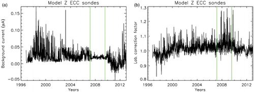
Next, we analyzed the time series of the ozonesonde pre-flight laboratory measurements appearing in Eq. (1) or in the Uccle correction algorithms. The deviations only occur in the free troposphere where ozone concentrations are lowest, so we first consider the background current measurements because the impact of these measurements on the final ozone amounts will be largest in this region. Figure 3a presents the background current time series, and it can be seen that this background current is very constant and low (±0.02 µA) during the anomalous 2007–09 period. Another interesting feature is that during the last years of our time series, we frequently measure a negative background current, which is then added to (instead of subtracted from) the measured current to obtain the ozone partial pressure (see Eq. (1)). This negative background current has also been measured in vacuum chamber experiments with ozonesondes and is believed to be a true physical property of the ozonesonde (Smit, personal communication, 2012). Even with this negative background current measured in the period after 2009, the final tropospheric ozone partial pressures are still lower than during the anomalous 2007–09 period. Moreover, the extreme low variability in the background current measurements in this anomalous period, compared with the periods before and after, points to the use of a very homogeneous and consistent series of ozonesondes with regard to the background current in those years.

Fig. 3 Time series of (a) the measured background currents and (b) ground calibration factors for the ECC model Z sondes at Uccle. The green vertical lines denote the beginning and end of the period of anomalous high tropospheric ozone values in the Uccle soundings; see Fig. 1d.

Another property of an ozonesonde measured in the laboratory before launch and used in Eq. (1) is the pump flow rate; lower pump flow rates give higher tropospheric ozone values because the decreasing efficiency of the pump with lower pressures (or temperatures) is negligible in the troposphere. However, during the 2007–09 period, the recorded times needed to pump 100 m³ of air fit perfectly in the overall time behaviour of this pump property (not shown here).

We now look at the time series of the ground calibration factors that are measured before launch (see Fig. 3b). As already explained in Section 2, at Uccle in the laboratory we compared the ozone sensor output with an imposed ozone amount of about 320 µg m⁻³ from a calibrated ozone source after a fixed time interval of 10 minutes. The calibration factor is then defined as the ratio of the ozone imposed by the calibrated ozone source to the ozone sensor output (in the same units), and an ozone sensor is accepted when this calibration factor lies in the range of 0.97 to 1.3. Contrary to the background current time behaviour during the anomalous period in Fig. 3a, the ground calibration factors in Fig. 3b are characterized by large variability and values at the high end of the range in the 2007–09 period. This means that, at the time of the pre-flight measurements, the amount of ozone measured by the ozonesonde sensor is too small with respect to the calibrated ozone source. This is rather puzzling because it contradicts the behaviour of the free tropospheric ozone during this period when the ozonesondes measure higher ozone concentrations than at nearby De Bilt and other European ozonesonde stations. This ground calibration factor appears in the pressure-dependent pump efficiency correction algorithm applied at Uccle, in which it serves as a scaling factor together with another scaling factor determined so as to match the on-site total ozone column measurement. We carried out a small experiment on the impact of this ground calibration factor via the correction algorithm on the final free tropospheric ozone column in the anomalous period by imposing a value of 1 (i.e., perfect agreement with the ozone calibration source) during this period. When these “adjusted” integrated ozone values between 3 and 8 km are then compared with their counterparts at De Bilt for quasi-simultaneous ozonesonde soundings (see Fig. 4), a small improvement is obtained (about 10% for the mean in the March 2007 to July 2009 time interval). This improvement is logical, because the raw (tropospheric) ozone values are now multiplied by scaling factors around 1 in the correction scheme instead of by factors larger than 1, and the corrected (tropospheric) ozone values are, therefore, smaller. Indeed, the scaling factor for the tropospheric ozone corrections in the pressure-dependent pump efficiency correction algorithm is primarily determined by the ground calibration factor and not by the total ozone column measurement; the opposite is true for stratospheric ozone values. Although at the high end of the range in March 2007 to July 2009, the ground calibration factors contribute only partially to the high tropospheric ozone values observed during this period.

Fig. 4 Differences in integrated ozone amounts in the 3–8 km layer between quasi-simultaneous ozone soundings at Uccle and De Bilt (see Fig. 1d) using different correction methodologies applied to the Uccle data. The red curve is the 50-day boxcar mean of these differences (in black), obtained by applying the correction algorithms developed at Uccle. Imposing a ground calibration factor equal to 1 during the anomalous period (marked by the green vertical lines), and applying the Uccle correction method to the Uccle data leads to the magenta boxcar mean of the differences (these latter are not shown here). The cyan curve represents the running mean of the differences with De Bilt after correcting the Uccle data with the standard algorithms.

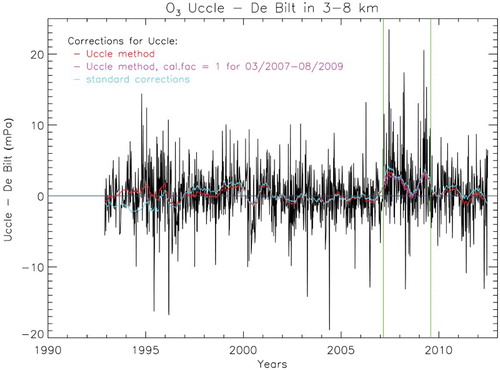
We subsequently investigated the sensitivity of the anomalous tropospheric ozone behaviour to the correction method applied at Uccle. Therefore, in Fig. 4, we also included the tropospheric ozone differences between the Uccle and De Bilt quasi-simultaneous ozone soundings, but with the Uccle ozone profiles corrected with the standard algorithms. From the figure, we can make two important statements. First, the anomalous tropospheric behaviour observed in the 2007–09 period in Uccle is independent of the data correction algorithms applied, or, to phrase it differently, the tropospheric deviations are larger than the impact of the corrections on the tropospheric ozone profile. Second, the correction algorithms developed at Uccle improve the agreement between the Uccle and De Bilt tropospheric ozone, not only in the time period of the anomalous Uccle behaviour (about 20% for the mean in the March 2007 to July 2009 time interval), but also over the entire time series, especially in the years before 1997, when the Brewer-Mast ozonesondes were used at Uccle. The comparison and impact of the different correction algorithms applied to the Uccle and De Bilt ozone profiles is the subject of a forthcoming paper; so, we will not go into further details on this matter at this point.

c Ozonesonde Batch Properties

The statistically detected change points in the Uccle and De Bilt tropospheric ozone differences accompany the first use of a new batch of ozonesondes. These are the ozonesondes with Z serial numbers starting with 10 (5 March 2007) and with Z serial numbers starting with 13 or 14 (7 August 2009). In Uccle, we normally order about half the ozonesondes needed for that year (150 soundings at a frequency of three times a week); the other half of the ozonesondes to be launched are recovered (i.e., re-tested and re-calibrated) ozonesondes. This practice results in a mixture of new and refurbished ozonesondes and in a mixture of ozonesonde batches used during a given period but with one batch dominant.

The analysis of the relation between the ozonesonde batches and the anomalous behaviour in Uccle is based on Table 2, which is a quantification of Fig. 1d, and lists the mean and standard deviations of the differences in integrated ozone in the 3–8 km layer for quasi-simultaneous soundings at Uccle and De Bilt for different combinations of batches and time periods. From Table 2a, we can link the high mean difference in the “bad period” (i.e., the period of anomalous behaviour defined here as occurring between 1 March 2007 and 1 August 2009) to the high mean differences of the ozonesonde batches (Z10…, Z11…, and Z12…) that were used mainly during this period. Indeed, those mean differences are all very high compared with the overall mean difference, and the mean difference for the bad period and the sum of the Z10… to Z12… batches is moreover significantly different from the overall mean difference according to a Student's t-test with the calculated t-value defined in Brandt (1970). For earlier and later batches, the mean differences between the Uccle and De Bilt data are closer to zero. Therefore, based on the discussion on Table 2a, we are tempted to conclude that three different “bad quality” batches of ECC ENSCI ozonesondes (with serial numbers Z10…, Z12…, and Z13…) are responsible for the anomalous behaviour detected during the 2007–09 period.

However, because of the practice of re-using ozonesondes, ozonesondes from a given batch have been used in both the “bad” and the “good” periods (i.e., outside the bad period). For instance, sondes with serial numbers Z10…, Z11…, and Z12… all had their first use during the bad period but were re-launched as recovered ozonesondes during the same period and also afterwards (during the good period). Consequently, we can split the mean differences of those batches into a mean difference for the bad period and a mean difference for the good period. The resulting mean differences (and their standard deviations) for this alternative sorting are summarized in Table 2b. This table shows that the “affected” batches seem to behave differently during the bad period than during the good period because both their mean differences and standard deviations are higher in the bad period, although the differences between these two periods are not statistically significant for the different batches shown in the table. Therefore, we could conclude that the high tropospheric O₃ values are not related to the ozonesonde batch, but we have more reasons to believe that the quality of the ozonesondes with serial numbers Z10… to Z12… was not inferior to earlier or later batches. First, three of the Z12… sondes were used in the most recent Juelich Ozone Sonde Intercomparison Experiment (JOSIE), and they did not give any observed discrepancies of the same magnitude in the vacuum chamber tests, although it should be mentioned that five of the eight experiments using those sondes were done when they were being re-used (Smit, personal communication, 2011). Second, let us for a moment assume that the reported high tropospheric values may have stemmed from some contamination of the ECC sensors during their manufacture. The argument could then be made that, although manufacturing specifications are very rigid, and tests are performed on batch sample sensors before they are released for sale, a number of different technicians are involved in the manufacturing process so if some problem occurred it may not have been documented (Komhyr, personal communication, 2011). The argument against this assumption is that ENSCI always manufactures ECC sensors in batches of 500 and ozonesondes from the same “suspect” batches^† were used in Payerne in the 2007–08 period without showing aberrant behaviour either in pre-flight measurements (Stübi, personal communication, 2013) or when compared with tropospheric ozone measurements taken at other European stations (Logan et al., 2012). Furthermore, about 60 ozonesondes from the same batch (Z10…) were launched from the high-latitude station at Scoresbysund, Greenland, between July 2006 and April 2007 which, once again, did not lead to aberrant tropospheric ozone measurements.

d Ozonesonde Descent Data

At Uccle, not only are the ascent data of an ozone sounding archived but the descent data, reprocessed and corrected with the same algorithms as the ascent data, are also archived. Until now, in this paper, only the ascent ozonesonde data have been used. These ascent data have a better vertical resolution than the descent data because the weather balloon rises more slowly than it descends. Additionally, data transmittance is more problematic at larger distances from the ground receiving station. As a consequence, the sonde descent profiles often lack data in the lowest atmospheric layers. Nevertheless, we will compare the lower quality Uccle descent data with the De Bilt ascent data in the free troposphere to gain additional information about the origin of the anomalous behaviour in the Uccle ozonesonde data between February/March 2007 and August 2009.

In Fig. 5a, the time series of monthly means of integrated ozone in the 3–8 km layer at De Bilt can be compared with the corresponding values for both the ascent and descent data at Uccle. When comparing the Uccle ascent and descent monthly mean data, it should be noted that the monthly means of the descent data have a larger variability than the ascent data because (i) the number of available descent soundings for this tropospheric layer is smaller than for the ascent soundings, since we demand that the descent profile reaches an altitude lower than 3 km, and (ii) the descent profile data have a lower vertical resolution than the ascent profile data. However, throughout the 2007–09 period, the Uccle sounding's descent data is in better agreement with the De Bilt values than its ascent data. This is not only true at the monthly mean level, but also for the quasi-simultaneous soundings at Uccle and De Bilt; during the March 2007 to July 2009 period, the mean difference with De Bilt is almost 30% lower for the Uccle descent data than for the ascent data.

Fig. 5 (a) Monthly mean time series of free tropospheric ozone at Uccle and De Bilt, as in Fig. 1b, along with Uccle ozonesonde descent data. (b) Time series of the differences of the same free tropospheric ozone values between an Uccle sounding's ascent and descent data, if the data transmittance during the descent was guaranteed below 3 km. The cyan curves shows the boxcar average (width = 50 days) of these differences; the red curve is the same as the red curve in Figs 1b and 4.

Subsequently, we calculated the differences in free tropospheric ozone between the ascent and descent parts of the Uccle ozone soundings, which are plotted in Fig. 5b. Globally, we can distinguish two periods during which there is a larger variability in the differences between the ascent and descent data with a tendency for higher values during the ascent than during the descent (the latter is demonstrated by the smoothed curve): first, the Brewer-Mast period before April 1997 and second the March 2007 to July 2009 period of anomalous tropospheric ozone behaviour. For comparison, the time-averaged differences between the Uccle ascent and De Bilt tropospheric ozone data is overplotted. The similarity between both curves, even in the details, is striking. It is apparent that the periods with large discrepancies between the Uccle and De Bilt data also have large discrepancies between the Uccle ascent and descent data. So it seems that the cause of the anomalous tropospheric ozone behaviour must be looked for in the ascent data primarily, or in conditions affecting ozonesonde measurements during the ascent.

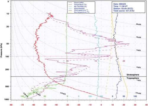
Figure 6 illustrates the differences between profiles gathered during the ascent and descent of the balloon launched on 25 March 2009. This is a sounding taken during the period of anomalous high tropospheric ozone values and is a typical example of a sounding during this period. When comparing the ascent (solid lines) and descent (dashed lines) profiles of this sounding, very good agreement can be detected between both profiles for all atmospheric variables except tropospheric ozone. Indeed, both stratospheric ozone profiles are reasonably consistent, even taking into account that the descent is much faster than the ascent, and because of the time lag of the ozonesonde sensor, there is a shift between both profiles. Also, the ozonesonde sensor does not have time to capture the fine structure of the ozone descent profile, including the magnitudes of local ozone maxima and minima. Hence, the ozonesonde sensor behaves similarly during the ascent and descent through the stratosphere. In the free troposphere, the ascent profile shows much higher ozone amounts than does the descent data, yet these latter might even be an overestimation because of the time lag effect. The specific reason for this discrepancy between the tropospheric ascent and descent data is still unclear, but two main causes can be considered—either an instrumental or a natural origin. One possible instrumental origin for the discrepancy is that the ozonesonde sensors used from 2007 to 2009 needed a longer conditioning time than the sensors from other batches. It could be expected that, after passing through the (ozone-rich) stratosphere, the ozonesonde sensors are conditioned properly and captured the lower ozone concentrations in the troposphere well. Conditioning of the ozonesonde sensors is extremely important for good functioning of the sensors and is, therefore, included in the standard operating procedures. First, four to five days before the day of the flight, the ECC sensor's Teflon pump and tubing should be conditioned with high ozone concentrations, at which time the ECC sensor should be filled with sensing solution. The instrument should then be set aside until the day of the flight. On the morning of the flight, the instrument should be prepared for flight by replacing the sensor cathode and anode electrolytes, followed by another ECC sensor conditioning with 5 µA ozone equivalent. However, we did not change the preparation procedures of the ozonesondes nor did the staff responsible for it during this period. An alternative explanation, of natural origin, is that the descent data (gathered at locations which are 50 to 100 km mean distance from Uccle, mostly to the northeast) trace other free tropospheric layers, more similar to those measured by the De Bilt ozonesondes, than in the immediate, urban area of Uccle. When looking at the wind speeds and directions in Fig. 6, we notice that wind speeds were high for this particular sounding, causing the ozonesonde to drift far from Uccle to the northeast, which, according to this alternative explanation, might then explain the high discrepancy between the ascent and descent tropospheric ozone values. However, we should mention that we did not find any correlation between the differences in the ascent and descent integrated ozone in the 3–8 km layer and the mean wind directions and mean wind speeds during the soundings.

Fig. 6 Vertical profiles of all measured atmospheric variables for the sounding launch on 25 March 2009. Solid lines denote the ascent profiles, and dashed lines show the descent.

e New Versus Recovered Ozonesonde Data

The hypothesis that the Uccle descent measurements show lower tropospheric values in the 2007–09 period because of the prolonged conditioning of the sensors can be tested by investigating the differences between the new and recovered Uccle ozonesonde (ascent and descent) measurements. The sensors of recovered ozonesondes are subjected to a longer, even in-flight, conditioning than new ozonesonde sensors. Table 3, similar to Table 2, but displaying the differences between Uccle and De Bilt for new and recovered ozonesondes separately, shows that for the ozonesonde series considered, smaller differences are obtained for the recovered ozonesonde sensors (group (a) in Table 3). However, these smaller differences with De Bilt for the recovered ozonesondes are mostly due to the ozonesondes with serial numbers Z10…, Z11…, and Z12…, launched during the 2007–09 period (compare group (b) with group (c) in Table 3). It is striking that for these serial numbers, the variability around the mean differences (standard deviation), is also reduced for the recovered versus the new ozonesondes. These two features point to a better and more consistent performance of the recovered ozonesondes for these batches for both the ascent and descent measurements. For the other ozonesonde batches considered (Z09…, Z13…, Z14…, and Z16…), the differences between the new and recovered ozonesondes are not at all significant, and no better agreement with the De Bilt values for the descent measurements is obvious.

Table 3. Statistical properties of the deviations in integrated ozone amounts in the 3–8 km layer for quasi-simultaneous observations at Uccle and De Bilt (as in Table 2), now calculated by discriminating between new and recovered ozonesondes, Uccle ascent and descent profile measurements, and for different combinations of the serial numbers Z09…, Z10…, Z11…, Z12…, Z13…, Z14…, and Z16 … . The “good” and “bad” periods are defined as before.

Group	Serial numbers		Ascent			Descent
			Mean	SD	n	Mean	SD	n
(a)	09 … ≤ Z < 17 …	New	1.55	19.96	122	1.33	17.61	82
	09 … ≤ Z < 17 …	Rec.	0.37	12.61	199	0.34	13.09	147
(b)	Z < 10 … or Z > 12 …	New	−0.42	6.10	55	−0.37	10.33	29
	Z < 10 … or Z > 12 …	Rec.	−0.17	10.39	87	0.19	8.67	57
(c)	10 … ≤ Z ≤ 12 …	New	3.18	25.67	67	2.26	19.36	53
	10 … ≤ Z ≤ 12 …	Rec.	0.79	14.03	112	0.44	16.00	90
(d)	10 … ≤ Z ≤ 12 …	New bad	3.21	26.01	66	2.31	19.61	52
	10 … ≤ Z ≤ 12 …	Rec. bad	0.53	19.97	60	0.73	18.74	45
	10 … ≤ Z ≤ 12 …	Rec. good	1.10	7.26	52	0.15	13.46	45

We also made a distinction between using new and recovered ozonesondes during the so-called good or bad periods (group (d) in Table 3). It appears that during the March 2007 to July 2009 period, the recovered ozonesondes from the Z10…, Z11…, and Z12… batches performed quite well in comparison with the De Bilt ozonesondes (small mean tropospheric ozone differences but at the cost of large standard deviations), in contrast to the new ozonesondes from the same batches. Recovered ozonesondes from the batches that were launched after July 2009 give rise to comparable mean differences with De Bilt (higher for the ascents, lower for the descents) and lower standard deviations. Hence, the table illustrates that the recovered ozonesondes of the “problematic” batches perform well in comparison with the De Bilt measurements. On the other hand, we were not able to test the performance of the new ozonesondes from these batches outside the bad period because only one ozonesonde fulfils these criteria. One last remark concerns the samples used in Table 3. We used all available quasi-simultaneous Uccle–De Bilt pairs and subsequently allocated the Uccle ozonesondes by batch number and first, second, or subsequent use. This means that a given ozonesonde might appear only once in the entire sample (e.g., new or recovered), or even more than once in the same sample (when re-used more than once). However, when restricting to ozonesondes that appear in both the new and recovered samples (thereby reducing the number of Uccle–De Bilt pairs considerably), identical conclusions are reached.

5 Natural ozone variability

A number of possible instrumental and operational factors that might cause the anomalies have been considered, but none were found that could provide a definitive explanation. Here, we will test the hypothesis of a real gradient in tropospheric ozone in the immediate vicinity of Uccle. As demonstrated by the analysis of the descent data, the term “immediate vicinity” should be taken literally, because the descent profiles reveal significantly lower tropospheric ozone amounts. The balloon flight paths from the launch at Uccle up to 5 km altitude reveal that (i) the vast majority of the balloons are within 15 km, to the (north)east, at that altitude, and (ii) the geographical distribution of these trajectories did not alter significantly from 2007 to 2009, compared with both earlier and later years. Therefore, one reasonable explanation is that ozone concentrations in the 3–8 km region of the atmosphere around Uccle increased in mid-2007 due to some local, new tropospheric O₃ pollution source such as, a new regional power plant or factory emitting NO_x, methane, CO, Volatile Organic Compounds (VOCs), etc. This disturbance in the concentration of ozone precursors might explain why the free tropospheric ozone increased drastically in the vicinity of Uccle but not in the tropospheric layers traced by the descending ozone sensors. Of course, for this assumption, another distortion in ozone precursor emissions should then also have occurred during 2009. We would then expect that changes in the emissions of ozone precursors would be reflected in boundary layer ozone amounts, but these agree very well with the De Bilt amounts. Therefore, we carefully analyzed surface observations of NO₂, CO, and VOCs at Uccle and three other stations in the Brussels metropolitan area (Elsene, Sint-Lambrechts-Woluwe, Sint-Stevens-Woluwe at 4, 9, and 11 km from Uccle, respectively) above which ozonesondes frequently cross the free troposphere. However, we could not find any correlation between the ozone precursor data for these stations and the anomalous high tropospheric ozone at Uccle in the 2007–09 period. Additionally, we compared the NO₂ tropospheric column overpass data at Uccle and De Bilt from the Ozone Monitoring Instrument (OMI; with a pixel size of 13 × 24 km at nadir) on the National Aeronautics and Space Administration's Aura satellite (Boersma et al., 2007). The 2004–13 time series for both stations are very similar and do not differ significantly from each other during the 2007 to 2009 period.

In addition, we would expect similar temporal behaviour of tropospheric ozone for stations located close to one another, like Uccle and De Bilt. Logan et al. (2012) argue in their paper that “the air masses above the sonde stations, airports, and alpine surface stations are not necessarily identical in their ozone content, and mountain sites are sometimes affected by boundary layer air and by local wind systems, but the data in Zbinden et al. (2006) and Gilge et al. (2010) suggest some degree of uniformity in ozone over central Europe on time scales of about a month” (see Logan et al., 2012, and references therein). However, to ascertain the origin of the anomalous high tropospheric ozone at Uccle, an analysis based on (the clustering of) back trajectories of the air parcels arriving at Uccle was undertaken. Such an analysis has been done for the boundary layer and the lower free troposphere at Uccle by Delcloo and De Backer (2008) for the 1969–2001 period (more details on the method can be found in their paper), and has now been extended up to 2010 and also for the years 2005 to 2010 for De Bilt. First, for every day of the year we calculated (at 12:00 utc) the five-day three-dimensional back trajectories starting at 500 hPa.

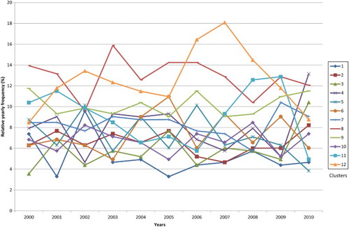
To reduce the number of air mass origins, we clustered the back trajectories according to the smallest normalized Euclidean distance criterion. The appropriate number of clusters is found by plotting the percentage difference between the sum of the root mean square deviations of each individual trajectory and its cluster mean. For instance, for the 2000–10 period at Uccle, 12 different clusters were retained by this method. The annual relative distribution of the different members over those 12 clusters is shown in Fig. 7. The maximum frequency of occurrence of cluster 12 (slow moving air masses from the southwest) in 2007 is remarkable because Delcloo and De Backer (2008) already mentioned that the highest ozone concentrations at 650 hPa in summer and spring are related to slow moving air masses over Europe. In 2008 and 2009, cluster 11 (fast longitudinal air masses coming from the United States) has the highest frequency of occurrence of all the years. However, keeping in mind that anomalous high tropospheric ozone values occur during all seasons for the February/March 2007 to August 2009 period, it should be noted from this figure that in the 2007–09 period, the distribution among the different clusters was not significantly different from the years before and after. Therefore, the back trajectory analysis could not confirm decisively that the air parcels arriving at Uccle originate from distinctly different regions during the 2007–09 period than in the time period before or after.

Fig. 7 Relative annual frequency of occurrence of trajectories in the different retained clusters for Uccle for 2000–10.

Next, we analyzed the clustering of the back trajectories and the distribution of the different members over the clusters for 2005 to 2010 for both Uccle and De Bilt. We chose this time period, because we can group it into three years showing the anomalous behaviour in tropospheric ozone at Uccle (2007–09) and three years with similar tropospheric ozone concentrations at both stations (2005–06, 2010). For both stations, 12 clusters were retained, of which 10 clusters are (nearly) identical. Uccle has one additional cluster with ascending air (coming from the southwest) and a cluster with fast moving air masses from the southwest, while De Bilt has an additional cluster with fast moving air masses from the west, and one with very slow moving local air masses. Also, the time variability of the frequency of occurrence of the cluster members is very similar for both stations. In particular, the above-mentioned maxima in the frequency of clusters occurred in the same years at De Bilt and Uccle for the same clusters. Hence, the cluster analysis reveals that the free tropospheric air arriving at both stations originates from quite similar geographical regions, and more so in the 2007–09 period. In this context, we want to make a final remark. A cluster analysis of back trajectories only gives a global image of the origin of the tropospheric air parcels. Looking at individual cases, high tropospheric ozone concentrations over Uccle compared with De Bilt might be explained by the back trajectories for Uccle crossing polluted areas such as London, the French port of Dunkirk, or the German industrial Ruhr area, while those for De Bilt cross north of London, above the English Channel, and less populated areas in the Netherlands before arriving at De Bilt.

6 Conclusions

In this paper, we confirmed the presence of a period, between approximately February/March 2007 and August 2009, during which anomalous high free tropospheric ozone concentrations were measured with the ozonesondes launched at Uccle. This finding has already been reported by Logan et al. (2012) and is investigated in more detail here, in particular by comparing the data with the nearby De Bilt ozonesonde station. It should also be emphasized that during the 2007–09 period, the pre-flight handling procedures for ozonesondes and the responsible operators, did not change. We could not identify one specific cause for these anomalies at Uccle but investigated several instrumental and environmental hypotheses.

Analyzing the pre-flight laboratory tests, we found that the measured background currents are very consistent and on the low side from March 2007 to August 2009, and the ozone amounts measured by the sensors were too small with respect to a calibrated ozone source. This might be interpreted as an indication of aberrant behaviour of the ozonesondes used during this period. Moreover, the beginning and end of the anomalous period actually coincides with the first use of new batches of ozonesondes. Indeed, the largest discrepancies between Uccle and De Bilt occurred during Uccle ascent ozone profiles and when using ozonesondes for the first time from three distinct batches (Z10…, Z11…, and Z12…). The discrepancies are smaller for the Uccle descent ozone profiles and when the ozonesondes from these batches were re-used. These two elements might point to the fact that the ozonesonde sensors from these specific batches needed a longer conditioning time in order to measure low ozone concentrations accurately in the free troposphere. Unfortunately, for the batches concerned, we could not completely decouple the effects of the ascent versus descent measurements and the use of new versus recovered ozonesondes from the anomalous period because other than during the March 2007 to August 2009 period, ozonesondes from these batches were not launched for the first time. Another argument against a possible conditioning issue during the first use of those specific batches is that ozonesondes from exactly the same batch have been used at Payerne and Scoresbysund without showing any anomalous behaviour in the free troposphere in their time series.

We also investigated the possibility of an environmental origin for the anomalous high tropospheric ozone values measured near of Uccle. Because the weather balloons carrying the Uccle ozonesondes were driven by the winds to similar free tropospheric regions in the 2007–09 period compared with the years before and after that period, we analyzed the concentrations of tropospheric ozone precursors at three surface stations in Brussels frequently crossed by ozonesondes during their ascent in the free troposphere. However, we could not detect any distinctive behaviour of those trace gases over any of those stations from 2007 to 2009. Additionally, column densities of tropospheric NO₂ measured by the OMI at Uccle and De Bilt are very similar, especially during the 2007–09 period. Finally, we also traced the origin of the tropospheric air at Uccle by calculating the back trajectories and subsequently clustering these. From this analysis, we found that (i) the origins of tropospheric air parcels at Uccle and De Bilt are not systematically different, and (ii) the air entering the free troposphere in Uccle during the 2007–09 period originates from similar geographical locations as in the years before and after.

A study to more thoroughly compare all the ozone profiles in the databases available for Uccle and De Bilt is being created. In that study, we will focus on the effect of each step in the different correction algorithms on the intermediate and final O₃ profiles at both sites and on the resulting trends calculated from the profiles at both stations. Because we are continually trying to improve our correction algorithms developed in-house, we will also investigate whether or not it is possible to use the tropospheric descent profile to develop a supplementary correction for the affected tropospheric ascent ozone profiles. For the time being, because the anomalous period is now past, this period will not affect a trend analysis based on the Uccle ozone sounding data if the most recent data are included and if a sufficiently long time series is used. It is also clear that the anomalous high ozone values at Uccle only arise in the free troposphere and not in the stratosphere or the boundary layer, which is in very good agreement with the De Bilt data.

Acknowledgements

Both R. Van Malderen and the ozone sounding program at Uccle are funded by the Solar-Terrestrial Centre of Excellence (STCE), a research collaboration established by the Belgian Federal Government through the action plan for reinforcement of the federal scientific institutes. We acknowledge the operators responsible for the ozone soundings at Uccle and De Bilt for their dedication throughout the years. We also want to thank Herman Smit for the very interesting discussions we had on this research and for his lead in the Ozonesonde Data Quality Assessment Program that gave us the occasion to attend workshops that were very instructive. We are grateful to Daan Hubert of the Belgian Institute for Space Aeronomy (BISA) for calculating the flight paths of the balloons launched at Uccle. We are indebted to the Belgian Interregional Environment Agency (IRCEL-CELINE) for kindly providing us with the ozone and ozone precursor data measured at different locations in Brussels. We acknowledge the free use of tropospheric NO₂ column data from the OMI sensor from www.temis.nl. Finally, we would like to thank the two anonymous reviewers for their very constructive feedback and suggestions.

Notes

^†Because ENSCI manufactured ECC sensors in batches of 500, not all ozonesondes with serial numbers starting with Z10… belong to the same production batch as our Z10… ozonesondes. Walter Komhyr, former CEO of ENSCI, kindly provided us with the names of the companies that received ozonesondes from the same batches.

References

- Boersma, K. F., Eskes, H. F., Veefkind, J. P., Brinksma, E. J., van der A, R. J., Sneep, M., … Bucsela, E. J. (2007). Near-real time retrieval of tropospheric NO2 from OMI. Atmospheric Chemistry and Physics, 7, 2103–2118. doi:10.5194/acp-7-2103-2007
- Brandt, S. (1970). Statistical and computational methods in data analysis (pp. 125–130). Amsterdam: North-Holland Publishing Company.
- De Backer, H. (1999). Homogenisation of ozone vertical profile measurements at Uccle. Royal Meteorological Institute of Belgium, Scientific and Technical Publication no. 7, ISSN D1999/0224/007. Retrieved from ftp://ftp.kmi.be/dist/meteo/hugo/publ/1999/o3prof.pdf
- De Backer, H., De Muer, D., & De Sadelaer, G. (1998). Comparison of ozone profiles obtained with Brewer-Mast and Z-ECC sensors during simultaneous ascents. Journal of Geophysical Research, 103(D16), 19641. doi:10.1029/98JD01711
- Delcloo, A. W., & De Backer, H. (2008). Five day 3D back trajectory clusters and trends analysis of the Uccle ozone sounding time series in the lower troposphere (1969–2001). Atmospheric Environment, 42(19), 4419–4432. doi:10.1016/j.atmosenv.2008.01.072
- European Union. (2008). Directive 2008/50/EC of the European Parliament and of the Council of 21 May 2008 on ambient air quality and cleaner air for Europe. Official Journal of the European Union.
- Gilge, S., Plass-Duelmer, C., Fricke, W., Karser, A., Ries, L., Buchmann, B., & Steinbacher, M. (2010). Ozone, carbon monoxide and nitrogen oxides time series at four alpine GAW mountain stations in central Europe. Atmos. Chem. Phys., 10, 12295–12316. doi:10.5194/acp-10-12295-2010
- Komhyr, W. D. (1969). Electrochemical concentration cells for gas analysis. Annales de Geophysique, 25, 203–210.
- Komhyr, W. D., & Harris, T. B. (1971). Development of an ECC ozonesonde (NOAA Technical Report ERL 200-APCL 18). Boulder, CO. U.S. Dept. of Commerce, National Oceanic and Atomospheric Administration, Environmental Research Laboratories.
- Lemoine, R., & De Backer, H. (2001). Assessment of the Uccle ozone sounding time series quality using SAGEII data. Journal of Geophysical Research, 106(D13), 14515. doi:10.1029/2001JD900122
- Logan, J. A., Staehelin, J., Megretskaia, I. A., Cammas, J.-P., Thouret, V., Claude, H., … Derwent, R. (2012). Changes in ozone over Europe: Analysis of ozone measurements from sondes, regular aircraft (MOZAIC) and alpine surface sites. Journal of Geophysical Research, 117(D9). doi:10.1029/2011JD016952
- Newman, P. A., Oman, L. D., Douglass, A. R., Fleming, E. L., Frith, S. M., Hurwitz, M. M., & Velders, G. J. M. (2009). What would have happened to the ozone layer if chlorofluorocarbons (CFCs) had not been regulated? Atmospheric Chemistry and Physics, 9(6), 2113–2128. doi:10.5194/acp-9-2113-2009
- Smit, H. G. J., & the Panel for the Assessment of Standard Operation Procedures for Ozonesondes (ASOPOS). (2011). Quality assurance and quality control for ozonesonde measurements in GAW (WMO/GAW Report No. 201). Geneva. World Meteorological Organization.
- Staufer, J., Staehelin, J., Stübi, R., Peter, T., Tummon, F., & Thouret, V. (2013). Trajectory matching of ozonesondes and MOZAIC measurements in the UTLS – Part 1: method description and application at Payerne, Switzerland. Atmospheric Measurement Techniques Discussions, 6, 3393–3406. doi:10.5194/amtd-6-3393-2013 doi: 10.5194/amt-6-3393-2013
- Steinbrecht, W., Claude, H., Schönenborn, F., Leiterer, U., Dier, H., & Lanzinger, E. (2008). Pressure and temperature differences between Vaisala RS80 and RS92 radiosonde systems. Journal of Atmospheric and Oceanic Technology, 25(6), 909–927. doi:10.1175/2007JTECHA999.1
- Stübi, R. (2012). Nairobi Data Analysis. 3rd Ozonesonde Data Quality Assessment Workshop, August 24–25, 2012, Toronto, Canada.
- Van Malderen, R., & De Backer, H. (2010). A drop in upper tropospheric humidity in autumn 2001, as derived from radiosonde measurements at Uccle, Belgium. Journal of Geophysical Research, 115(D20). doi:10.1029/2009JD013587
- WMO (World Meteorological Organization). (2011). Scientific assessment of ozone depletion: 2010 (Global Ozone Research and Monitoring Project – Report No. 52). Geneva, Switzerland. World Meteorological Organization.
- Zbinden, R. M., Cammas, J.-P., Thouret, V., Nedelec, P., Karcher, F., & Simon, P. (2006). Mid-latitude tropospheric ozone columns from the MOZAIC program: Climatology and interannual variability. Atmos. Chem. Phys., 6, 1053–1073. doi:10.5194/acp-6-1053-2006