Reducing Drift and Bias of a Global Ocean Model by Frequency-Dependent Nudging

Abstract

Frequency-dependent nudging is applied to a coarse resolution (nominal 1°) global ocean model to suppress its drift and bias, and the impact of the nudging on the skill of the model is assessed. The nudging is applied to temperature and salinity in frequency bands centred on 0 and 1 cycles per year. As expected, the nudging significantly reduces the biases in the long-term mean and annual cycle of temperature, salinity, and sea level. By comparing the simulated (i) sea surface temperature with operational analyses based on observations, (ii) vertical profiles of temperature and salinity with observations made by Argo floats, and (iii) sea level with altimeter observations, it is shown that the skill of the model in simulating variability about the annual cycle is also improved. The potential benefit of applying frequency-dependent nudging to the ocean component of a coupled atmosphere–ocean model is discussed.

Résumé

[Traduit par la rédaction] Nous appliquons un poussage dépendant de la fréquence à un modèle océanique planétaire de résolution grossière (nominale 1°) pour supprimer sa dérive et son biais et nous évaluons l'effet du poussage sur l'habileté du modèle. Nous appliquons le poussage à la température et à la salinité dans des bandes de fréquences centrées sur 0 et 1 cycle par année. Comme attendu, le poussage diminue considérablement les biais dans la moyenne à long terme et le cycle annuel de la température, de la salinité et du niveau de la mer. En comparant les valeurs simulées (i) de la température de la surface de la mer aux analyses opérationnelles basées sur des observations, (ii) des profils verticaux de température et de salinité aux observations faites par des flotteurs Argo et (iii) du niveau de la mer aux observations altimétriques, il apparaît que l'habileté du modèle à simuler la variabilité en ce qui a trait au cycle annuel est aussi améliorée. Nous discutons des avantages possibles de l'application d'un poussage dépendant de la fréquence à la composante océanique d'une modèle couplé atmosphère–océan.

KEYWORDS:

• global ocean model
• drift
• bias correction
• nudging
• skill assessment

1 Introduction

The present study is part of a larger, ongoing effort to build an operational coupled atmosphere–ocean forecast system for Canada as part of a multi-departmental initiative involving Environment Canada, Fisheries and Oceans Canada, and the Department of National Defence. The forecast system is based on the Environment Canada Global Environmental Multi-Scale (GEM) atmospheric model and the Mercator-Océan Nucleus for European Modelling of the Ocean (NEMO) data assimilation and forecast systems from France. The GEM atmospheric model (Côté et al., 1998) is presently being used for operational weather forecasting at the Canadian Meteorological Centre (CMC). The coupling of the GEM atmospheric model and the NEMO ocean model is supported by the Canadian Operational Network of Coupled Environmental PredicTion Systems (CONCEPTS) which is a new inter-departmental initiative to improve the forecast skill of coupled systems in the short-, medium- and long-range time scales (with corresponding lead times of hours to a season).

One of the problems that arose with the initial runs of the ocean component of the coupled system (spun up over a decade) is that they exhibited significant drift and bias errors. These are common problems with many atmospheric and ocean models (e.g., Bleck, 2002; Dee, 2005; Halliwell, 2004; Huddleston, Bell, Martin, & Nichols, 2004), and they have the potential to seriously degrade the quality of the forecasts made by a coupled system. Many factors can contribute to drift and bias (e.g., poor parameterization of subgrid-scale processes and inaccurate surface boundary conditions), and even the most comprehensive general circulation models are not immune to such problems, let alone global models with relatively coarse horizontal resolution. Biases can result in inaccurate large-scale circulation features and associated instabilities, which can degrade the accuracy of short-term forecasts. A related problem is that without an effective method for suppressing drift and bias, the assimilation of observations may result in initialization shock which can prevent a forecast system from achieving its optimal forecast skill (Balmaseda, 2004; Segschneider, Balmaseda, & Anderson, 2000; Vidard, Anderson, & Balmaseda, 2007).

The problem of model bias has been widely recognized in recent years, and several approaches have been developed to suppress it (e.g., Balmaseda, Dee, Vidard, & Anderson, 2007; Chepurin, Carton, & Dee, 2005; D'Andrea & Vautard, 2000; Dee & da Silva, 1998; Griffith & Nichols, 1996, 2000; Kamen & Su, 1999; Thiebaux & Morone, 1990). Thompson, Wright, Lu, and Demirov (2006) developed a simple scheme for suppressing model bias that involves in-line nudging of the model's state towards observed seasonal climatologies of temperature and salinity in specific frequency bands; outside these bands the model evolves freely. By choosing the central frequencies of the nudged bands to coincide with the dominant frequencies of the observed climatology (e.g., 0 and 1 cycles per year) it is possible to reduce seasonal biases while allowing the non-seasonal variability to evolve more freely than conventional nudging would allow. The scheme has subsequently been applied with some success to regional, eddy-permitting ocean models (e.g., Lu, Wright, & Yashayaev, 2007; Stacey, Shore, Wright, & Thompson, 2006; Wright, Thompson, & Lu, 2006; Zhu, Demirov, Dupont, & Wright, 2010).

In this study we explore the effect of frequency-dependent nudging on the ocean component of the new Canadian global coupled forecast system. We focus on a relatively coarse version of the global ocean model (grid spacing of approximately 1°) which, as mentioned above, is known to develop significant temperature and salinity biases when integrated for a decade or longer without data assimilation. The approach used in the present study is to run the ocean model with and without the frequency-dependent nudging, examine the change in the seasonal biases, and also assess the realism of variability about the annual cycle through comparison with independent ocean observations (e.g., altimetric observations of sea level). To our knowledge this is the first time frequency-dependent nudging has been applied to a global ocean model and we see it as an initial step in the implementation of frequency-dependent nudging of the ocean component of the global coupled system.

The paper is organized as follows. The global ocean model and frequency-dependent nudging are described in Section 2. The observed seasonal climatology and additional observations for model validation are described in Section 3. The impact of the frequency-dependent nudging on the model-simulated seasonal climatology is quantified in Section 4, and its impact on variability about the annual cycle is quantified in Section 5. A summary and suggestions for future work are provided in Section 6.

2 The ocean model and bias correction methodology

The ocean model is based on version 2.3 of NEMO (http://www.nemo-ocean.eu/). It includes version 9 of the finite difference, hydrostatic, primitive equation ocean model (Ocean PArallelise (OPA); Madec, Delecluse, Imbard, & Levy, 1998), and version 2 of the sea ice model (Louvain-la-Neuve Sea Ice Model (LIM); Fichefet & Morales Maqueda, 1997). The model grid follows the global tripolar ORCA configurations that are widely used by NEMO investigators of one-degree global ocean modelling (e.g., Barnier et al., 2006). Here the coarse-resolution grid ORCA1 has a nominal resolution of about 1° extending from 78°S to 90°N, with a reduced latitudinal grid spacing of about 1/3° near the equator. The vertical dimension is discretized using 50 geopotential levels, with thickness increasing from 1 m at the surface to 450 m near the bottom.

The model is initialized using the January climatology of temperature and salinity of Levitus (1998) and is driven by two sets of atmospheric forcing. From 1992 to 2001, the model is driven by version 2 of the forcing data compiled for the Coordinated Ocean-ice References Experiments (CORE; Large & Yeager, 2004, 2009). From 2002 to 2007, the model is driven by a dataset based on CMC's operational Global Deterministic Prediction System, rerun daily with a horizontal resolution of 33 km (Smith et al., 2013). Surface momentum, heat, and freshwater fluxes are calculated using the CORE bulk formulae (Large & Yeager, 2004).

To explain the approach used to suppress the drift and bias of the model letdenote the one step ahead forecast of the analyzed model state x_t at time t. The vector valued, non-linear function ϕ_t depends on the dynamics of the model. Nudging toward an observed seasonal climatology (c_t ) is implemented by adding a restoring term to the above update equation as follows:where γ is a nudging coefficient, and ⟨ ⟩ denotes a quantity that has been bandpass-filtered to (i) pass almost unchanged variations with frequencies in the vicinity of 0 and 1 cycles per year, and (ii) almost completely suppress variations outside these frequency bands. (Note that, for simplicity, we have assumed the seasonal climatology is available for every element of the state vector. This is not required in practice. In the present study we will nudge only temperature and salinity.)

Because this method allows the model's seasonal climatology to be nudged toward an observed seasonal climatology while leaving the short-term variability to evolve freely according to the model's dynamics and external forcing, we will refer to the nudging scheme described above as frequency-dependent nudging. The implementation of frequency-dependent nudging requires a computationally efficient and effective filter with zero-phase lag at climatological frequencies. In this study, we use the filter proposed by Thompson et al. (2006). It is shown that the phase of the filter is zero and the amplitude is one at the climatological frequencies. A plot of the amplitude and phase of the filter is given in Figure 11 of Thompson et al. (2006). Practical details on the technique, including the transfer function of the filter, are given in Thompson et al. (2006) and Wright et al. (2006).

The implementation of frequency-dependent nudging involves the specification of two parameters (Thompson et al., 2006). One parameter κ is the width of the frequency bands over which the model is to be nudged. The reciprocal of κ controls the spin-up time of the in-line filter. We set this parameter to three years. The same parameter also controls the extent to which the model's mean and annual cycle for a given year can vary about the observed seasonal climatology. The other parameter is γ; it controls the strength of the nudging. The reciprocal of γ is the relaxation time scale and we set it to correspond to one month. A number of sensitivity studies with different parameter values were performed to assess the impact of these parameters on the model, and the results were not strongly dependent on the exact parameter choices.

To assess the impact of frequency-dependent nudging, two runs of the model are performed. The only difference between the runs is the use of frequency-dependent nudging. The control (CTL) run does not include any nudging. It should be noted that (i) ocean-only models usually include a restoring (nudging) term for sea surface salinity if there is no explicit correction for surface freshwater fluxes, and (ii) the use of bulk formulae for the air-sea fluxes implies an implicit control of sea surface temperature through the dependence of the fluxes on surface air temperature. The frequency-dependent nudged (FDN) run is nudged to an observed climatology (defined below). The model output was stored in the form of 10-day averages every 10 days. The comparison of the control and nudged runs, and their comparison with independent observations, is based on data for the period 2002 to 2007.

3 The observed seasonal climatology and observations for validation

The Commonwealth Scientific and Industrial Research Organization (CSIRO) produce the observed seasonal climatology of temperature and salinity, the CSIRO Atlas of Regional Seas (CARS2009) towards which the model is nudged. This climatology is derived from a quality-controlled archive of all available historical subsurface ocean property measurement profiles (e.g., World Ocean Database 2005, surface-pressure-corrected Argo global archives, and World Ocean Circulation Experiment (WOCE) Global Hydrographic Program v3.0). Because data availability has increased significantly in recent years, the CARS climatology is biased towards the more recent ocean state. Note the climatology is based on observations from the model simulation period. This means that the simulations are not true forecasts because future information is used. However, the only information used by the frequency-dependent nudging is the long-term seasonal cycle and, by definition, this changes slowly with time.

Gridded global fields of sea surface temperature, sea level, and vertical profiles of temperature and salinity, are used to assess the accuracy of the model runs. The observations used in this study cover the period 2002 to 2007. The datasets are described below.

The sea surface temperature fields were generated by CMC using the methodology of Brasnett (2008). The fields are available daily with global coverage and a grid spacing of 0.2°. They have been averaged to ORCA1 grids for comparison with the model. The fields are based on a near real-time analysis of in situ observations and retrievals from one microwave (Advanced Microwave Scanning Radiometer-Earth observing system (AMSR-E)) and three infrared (Along Track Scanning Radiometer (ATSR), Advanced Along Track Scanning Radiometer (AATSR), and Advanced Very High Resolution Radiometer (AVHRR)) satellite-borne sensors. The analysis uses statistical interpolation to update the fields daily, with the analysis from the previous day used as the background. The global average root mean square error is less than 0.4°C.

The sea surface height anomaly fields were generated by Ssalto/Duacs and distributed by Aviso, with support from Centre National d’Études Spatiales (CNES; http://www.aviso.oceanobs.com/duacs/). These products were based on altimeter data from the TOPEX/Poseidon, Jason-1, European Remote Sensing 1/2 (ERS1/2), and ENVISAT satellite missions and computed with respect to a seven-year mean (Ducet, Le Traon, & Reverdin, 2000). The fields are provided weekly with a global coverage and a grid spacing of 1/3° and are averaged to the ORCA1 grid for comparison with the model. To include the long-term mean, and to calculate surface geostrophic currents, the mean dynamic topography product MDT_CNES-CLS09 was added to the gridded sea level fields. This mean dynamic topography was produced by Collecte Localisation Satellites (CLS) Space Oceanography Division and distributed by Aviso, with support from CNES (http://www.aviso.oceanobs.com/).

The observed vertical profiles of temperature and salinity used in this study were made by conductivity-temperature-depth recorders, bathythermographs, and autonomous profilers launched and maintained by the Argo program. The profiles were downloaded from the National Oceanographic Data Center website (http://data.nodc.noaa.gov/gtspp/, hereinafter referred to as Argo profiles).

The ocean model was nudged to the CARS seasonal climatology and the model simulations compared with the global fields of observed sea surface temperature and sea level, as well as vertical profiles of temperature and salinity. Note that the observed sea level fields were not assimilated by the model so they provide a completely independent set of observations for model validation. The situation is less clear for the gridded fields of surface temperature because the observations on which they are based were used to calculate the model's surface fluxes and the seasonal climatology. Similarly the vertical profiles of observed temperature and salinity cannot be considered to be a completely independent dataset because, as discussed above, they too were used to define the seasonal climatology to which the model is nudged. We discuss these limitations later in the paper.

4 Impact of frequency-dependent nudging on the mean and annual cycle

Frequency-dependent nudging was designed to nudge a model toward an observed seasonal climatology in the vicinity of specific central frequencies. In this section we check how effectively we have nudged the long-term mean and annual cycle of our 1° global ocean model towards the CARS seasonal climatology.

a Surface Temperature and Salinity

We first compare the long-term means of sea surface temperature and salinity from the control run with the corresponding long-term means of the observed climatology. The surface temperature from the control run (Fig. 1a) is too warm in most regions (e.g., the bias exceeds 1°C over much of the eastern Pacific and Atlantic oceans). There are large biases in the vicinity of strong ocean currents (e.g., more than 3°C in the Gulf Stream, Antarctic Circumpolar Current, and Kuroshio Extension and −3°C in the vicinity of the Labrador Current). The surface salinity of the control run (Fig. 1b) also has significant biases of almost 1 over large parts of the global ocean.

Fig. 1 The long-term bias of sea surface temperature and salinity relative to the CARS climatology. (a) and (b) Control run and (c) and (d) nudged run. Positive values indicate that the simulated temperature or salinity is too high relative to the mean of the observed climatology. Temperatures are in degrees Celsius.

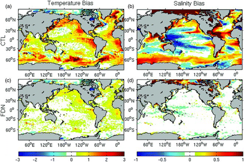
As expected, frequency-dependent nudging reduces the long-term bias of surface temperature and salinity (Figs 1c and 1d, respectively). After nudging, there are only a few areas where the bias of sea surface temperature exceeds 1°C. The bias of sea surface salinity has also been reduced significantly and is less than 0.1 in most regions. We note that, for temperature, there are large biases in Hudson Bay while the bias in the Arctic area for salinity is large for both simulations. The reason for these large biases is that the model does not perform well in ice-covered areas. Although the biases were significantly reduced in the nudged run, they are still relatively large in these areas.

We note that instead of frequency-dependent nudging, a conventional restoring of sea surface salinity would also reduce the time-mean bias. However, this method has the known deficiency of suppressing model-simulated variability and introducing phase errors for the seasonal cycle (Pierce, 1996). We further note that for the control run, the use of bulk formulae in calculating surface heat fluxes did not eliminate the bias in sea surface temperature.

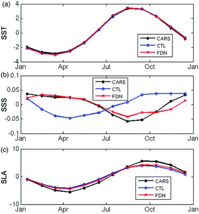
To illustrate the performance of frequency-dependent nudging at a period of one year, seasonal cycles of surface temperature and salinity were spatially averaged over the North Atlantic (10°W to 70°W, 15°N to 45°N). Both runs accurately reproduce the observed seasonal variation of surface temperature for this area (Fig. 2a). Large seasonal biases of surface salinity are evident in the control run; the phase of the simulated annual cycle of surface salinity differs from the observed cycle by about 180° (Fig. 2b). By way of contrast, the seasonal variation of surface salinity of the nudged run is much closer to observations, apart from a small bias in autumn and winter. Figure 2c for sea level is discussed later.

Fig. 2 Seasonal variation in (a) sea surface temperature, (b) sea surface salinity, and (c) sea level anomaly for the North Atlantic, averaged over the region 10°W to 70°W, 15°N to 45°N. The black curve corresponds to the observed climate; the blue curve corresponds to the control run; and the red curve is for the nudged run. The dots correspond to monthly means. The long-term mean value has been removed from each time series.

b Sea Level and Surface Geostrophic Circulation

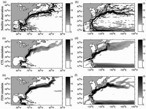
A problem with many low-resolution models of the North Atlantic (e.g., Maltrud & McClean, 2005) is unrealistic separation of the Gulf Stream at Cape Hatteras. Figure 3 shows the speed of the mean surface geostrophic velocity calculated from spatial gradients of the observed mean dynamic topography (described in Section 3) and mean sea level from the control and nudged runs. It is clear that the Gulf Stream in the control run separates too far north and is too wide between 48°W and 30°W (compare Figs 3a and 3c). The nudged run is a significant improvement (Fig. 3e). Similar conclusions hold for the Kuroshio Extension region (compare Figs 3b, 3d and 3f). More specifically, the control run fails to reproduce the observed separation point and the path of the eastward flowing Kuroshio Extension jet. The nudged run is in much closer agreement with observations (compare Figs 3b and 3f). There is, however, still evidence of overshoot close to the separation point, and the Kuroshio Extension jet is too broad and weak. Given the low resolution of the model, it is not surprising that both simulations fail to accurately represent these western boundary currents.

Fig. 3 Speed of the mean surface geostrophic flow calculated from spatial gradients of mean sea surface height. (a) and (b) Satellite observations, (c) and (d) control run and (e) and (f) nudged run. The left panels are for the Gulf Stream region and the right panels are for the Kuroshio Extension region. Speeds are in cm s⁻¹.

The seasonal variation of sea level averaged over the North Atlantic is shown in Fig. 2c for the two model runs and the observations. Both runs underpredict the amplitude of the observed seasonal cycle by about 1 cm. The difference between the control and nudged runs is small.

c Subsurface Temperature and Salinity

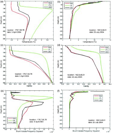
To verify the performance of the two simulations at the subsurface level, we compared the simulated temperature and salinity with the Argo profiles. To make sure the model and Argo profiles are comparable, the Argo observations were first averaged over the model grid cells in every 10-day window, and the averaged observation was only used if the number of profiles in the grid cell exceeded five. In this way, the observations and model results have the same spatial and time resolutions. We selected two individual cases to compare the simulated temperature and salinity profiles with the corresponding Argo profiles, one of which was taken from the subpolar area where the model performs relatively poorly; the other was selected from the region where the model performs well. It is clearly shown in Fig. 4 that the nudged run is much closer to the observations than the control run in both of the cases. We then calculated the standard deviation of the differences between the observed and simulated profiles at specific depths, as well as their correlations. Note that both of these statistics are influenced by errors in the annual cycle and also variations about the annual cycle.

Fig. 4 Comparison of observed and simulated vertical profiles of temperature and salinity. (a) Temperature profile (176°W, 55.8°N) on 5 April 2004; (b) temperature profile (163°W, 48°N) on 25 July 2004; (c) salinity profile (176°W, 55.8°N) on 5 April 2004; (d) salinity profile (163°W, 48°N) on 25 July 2004; (e) squared Brunt-Vaisala frequency profile (176°W, 55.8°N) on 5 April 2004; and (f) squared Brunt-Vaisala frequency profile (163°W, 48°N) on 25 July 2004.

The standard deviation of the difference between the observed and simulated profiles is shown in the top panels of Fig. 5 as a function of depth. To put these results into perspective, we also calculated standard deviations of the difference between the observed profiles and the seasonal climatology to which the nudged run was nudged (i.e., the CARS climatology). The standard deviations of the nudged temperature errors are smaller than climatology over the top 500 m (red line, top left panel). Overall, the standard deviations of the control temperature errors are slightly lower than climatology but higher than the nudged run. The result for salinity (top right panel) shows that the nudged run outperforms the control run, and the climatology as a predictor, at all depths. We note that the control simulation is worse than the observed seasonal climatology above 100 m.

Fig. 5 Comparison of observed and simulated vertical profiles of temperature and salinity as a function of depth. (a) and (b) Standard deviation of the differences between the observations and simulations, based on all available Argo profiles from the global ocean for the period 2002 to 2007. Observations from all seasons were used. The standard deviation of the difference between the observed profiles and the observed seasonal climatology is also shown for reference. (c) and (d) Correlation between the observations and simulations from the control and nudged runs.

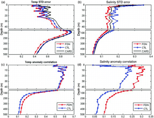
The correlation between observed and simulated temperature is highest for the nudged run at all depths (red line, bottom left panel, Fig. 5). The correlation between the observed and simulated salinity is also highest for frequency-dependent nudging (red line, bottom right panel) although we note that the correlations are quite low (less than about 0.3 at all depths).

The standard deviations and correlations presented in Fig. 5 are based on all available data for the global ocean. We now focus on the tropical Pacific Ocean. We chose this region mainly because it plays an important role in ocean–atmosphere interactions (Rasmusson & Carpenter, 1982) and the transport of heat (e.g., Bonjean, 2001; Picaut, Ioualalen, Menkes, Delcroix, & McPhaden, 1996) and salt (e.g., Delcroix & Picaut, 1998). We also chose this region because simulating its climate and variability has proven a challenge for global climate models (e.g., Guilyardi et al., 2004; Latif et al., 1994; Lin, 2007; van Oldenborgh, Philip, & Collins, 2005). We focus below on an east–west section along the equatorial Pacific Ocean, averaging profiles between 10°S and 10°N.

The long-term temperature bias of the control run exceeds 1.5°C between 50 and 150 m in the eastern tropical Pacific (Fig. 6a). In the western basin, and depths between 100 and 500 m, there is a strong negative bias that reaches −1.5°C at 150 m. The long-term salinity bias (Fig. 6b) indicates that the control simulation is too fresh over the top 50 m and too salty between 50 and 150 m. Between about 200 and 400 m the control salinity is about 0.2 lower than the observed long-term mean in the western part of the tropical Pacific.

Fig. 6 Long-term bias of the two simulations along the equatorial Pacific. Results are based on differences between observed and simulated profiles of temperature and salinity made within 10 degrees of the equator. (a) and (b) Control run and (c) and (d) nudged run. The temperature bias (a) and (c) is in degrees Celsius.

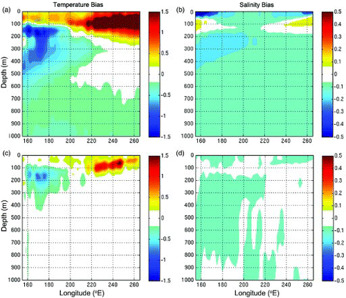
The long-term temperature and salinity biases of the nudged run are significantly lower than the biases of the control run, as expected. The temperature bias (Fig. 6c) is below 0.2°C everywhere except at depths between 50 and 200 m, where both runs perform relatively poorly. We note, however, that the bias near the thermocline is significantly reduced in the nudged run. The long-term salinity biases greater than 0.1 are almost completely eliminated (Fig. 6d) by the frequency-dependent nudging.

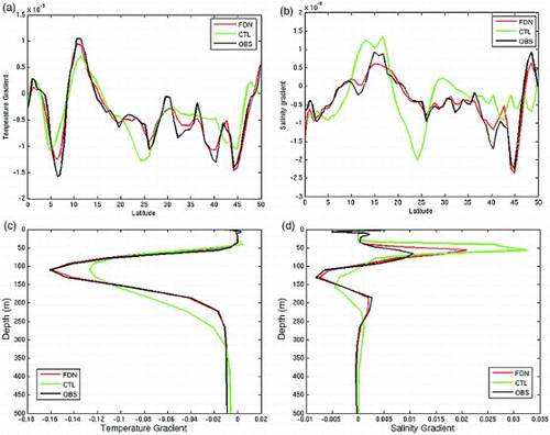
Temperature and salinity gradients play an important role in driving the dynamics and thermodynamics of the ocean so we also verify the model's performance by examining the temperature and salinity gradients. Figure 7 shows the meridional gradients of the long-term mean temperature and salinity at 110 m depth along 180°E. The horizontal gradient is defined as the change in temperature or salinity over the distance between two adjoining grid cells along the meridian. It is shown that the horizontal gradients calculated from both simulations are similar to the climate observations, but the nudged run captures more of the details of the gradient curves. The vertical gradients are shown in Figs 7c and 7d. They lead to a similar conclusion: the nudged run outperforms the control run at almost all depths, indicating that the nudged run improves the representation of vertical stratification.

Fig. 7 Effect of frequency-dependent nudging on long-term mean horizontal and vertical gradients. (a) Horizontal temperature gradient along 180°E at 110 m depth (°C m⁻¹); (b) horizontal salinity gradient along 180°E at 110 m depth (m⁻¹); (c) vertical temperature gradient at (180°E, 10°N) (°C m⁻¹); and (d) vertical salinity gradient at 180°E, 10°N (m⁻¹).

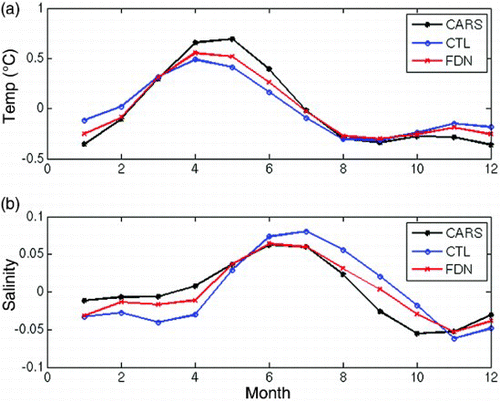
The seasonal variation in temperature and salinity, averaged between 10°S and 10°N and depths between 200 and 400 m, for the equatorial Pacific region is shown in Fig. 8. Overall, the seasonal variations in temperature and salinity from the nudged run are closer to observations than the control run, as expected. (The seasonal variation in temperature from the control run is smaller than observed, and the seasonal variation in salinity is too large.)

Fig. 8 Monthly means of subsurface temperature (a) and salinity (b) averaged between 10°S and 10°N in the equatorial Pacific and between depths of 200 and 400 m. The long-term mean has been removed. The observed climatology (black line) is based on the CARS climatology. The control and nudged runs are shown by the blue and red lines, respectively. Temperatures are in degrees Celsius.

In summary, the results presented in this section confirm that frequency-dependent nudging of the global model performs as expected. It reduces the long-term mean and seasonal biases in the nudged variables (temperature and salinity) and also brings sea level and mean surface geostrophic flow into closer agreement with observations. These results are consistent with other regional applications of frequency-dependent nudging (e.g., Wright et al., 2006).

5 Impact of nudging on variations about the annual cycle

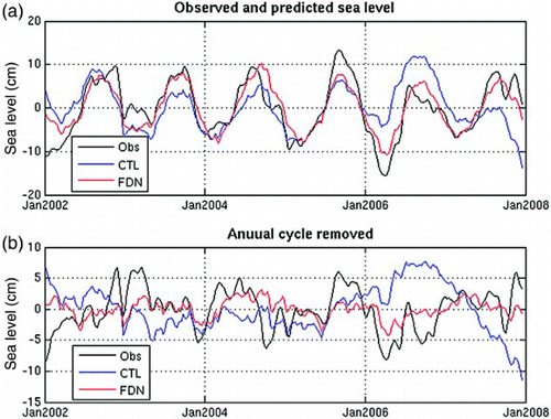
To motivate the following discussion on variability about the annual cycle we present, in Fig. 9a, the time variation of observed sea level and simulations from the control and nudged runs for a representative location in the eastern North Pacific (128.3°W, 41.5°N). (The location is off the coast of California.) Given that the eddy kinetic energy is relatively low in this region, it is more likely that the low-resolution model will be able to represent the variation in sea level at the selected location. In Fig. 9 the nudged run (red line) agrees most closely with observations (black line) than with the control run (blue line). This is not surprising because the model has been nudged to the observed mean and annual cycle of temperature and salinity and thus the observed density field and steric height. The variations in sea level (Fig. 9b), after removal of the long-term mean and annual cycle by least squares regression, show that the nudged run outperforms the control run on time scales exceeding one year. In particular, the control run generates large sea level changes of the order of 10 cm in 2006 and 2008 that are approximately out of phase with the observed changes. The performance of the control and nudged runs at higher frequencies is harder to assess by visual examination of Fig. 9b. We return to this point later.

Fig. 9 A representative time series of observed and simulated sea level from 128.3°W, 41.5°N in the eastern North Pacific. (a) Observed sea level (black line), simulations from the control run (blue line), and nudged run (red line). The long-term mean has been removed. (b) Same as (a) but after removal of the annual cycle by least squares regression. The sea levels are in centimetres.

The rest of this section extends the discussion on variability about the annual cycle to cover the entire model domain. We also assess the performance of the two runs at both low frequency (periods longer than one year) and high frequency (periods shorter than one year). We focus primarily on sea level because it is a variable of high practical and scientific relevance, and sea level observations were not used, implicitly or explicitly, in generating the two model runs. Observed sea level also has almost global coverage, and the availability of gridded fields greatly simplifies the quantitative evaluation of the two runs. We also briefly discuss sea surface temperature but note that this is not a truly independent variable because it is used to specify the surface forcing.

The standard deviations of low frequency variations of observed sea level (top left panel, Fig. 10) reach 5 cm in regions with strong currents (e.g., Gulf Stream, Kuroshio Extension jet, Aghulas Retroflection, and Antarctic Circumpolar Current) and regions known to have strong interannual variability (e.g., the tropical Pacific and Indian oceans). Away from these regions the standard deviation is typically less than about 1 cm. The corresponding map for the control run (middle left panel) shows that the entire domain is filled with low frequency variations with standard deviations exceeding about 2 cm; these variations are caused primarily by the drift of the model (see Fig. 9b). The standard deviation of the low frequency variations of the nudged run are in closer agreement with observations (compare top and bottom left panels, Fig. 10). Away from strong currents, the low frequency standard deviation of the nudged run is less than about 1 cm, reflecting the suppression of the drift of sea level that inflated the low frequency standard deviation of the control run. The nudged run also reproduces the elevated standard deviations of low frequency variability that are observed in the tropical Pacific and Indian oceans. In regions with strong currents the nudged run underestimates the low frequency variability. Such variability in observations is likely caused by long life-cycle eddies, eddy-mean flow interaction, or meandering of narrow currents. The present model's resolution of 1° is too coarse to simulate these processes.

Fig. 10 Standard deviation of low and high frequency variations of sea level after removal of the annual cycle. (a), (c), and (e) Low frequency standard deviations. (b), (d), and (f) High frequency standard deviations. (a) and (b) are for observations; (c) and (d) and (e) and (f) are for the control run and nudged run, respectively. Standard deviations are in centimetres.

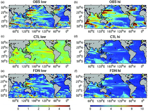
The standard deviations of the high frequency variations of observed sea level (top right panel, Fig. 10) exceed 20 cm in regions with strong, unstable currents (e.g., Gulf Stream, Kuroshio Extension jet, Aghulas Retroflection, and Antarctic Circumpolar Current). Both runs fail to reproduce these elevated standard deviations (middle and bottom panels) although there is some similarity in the spatial patterns. We again attribute this discrepancy to the low resolution of the ocean model that results in its failure to simulate meandering of mid-ocean jets and the generation and movement of ocean eddies. The high frequency standard deviation of the control and nudged runs (compare middle and bottom right panels) are quite similar, confirming that frequency-dependent nudging has a small impact on sea level variance at periods less than one year.

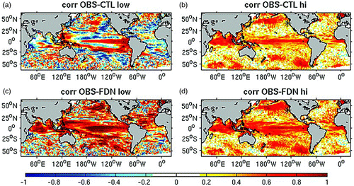
The performance of the two runs has also been assessed using the correlation between observed and simulated sea levels. The correlations were calculated separately for the low and high frequency components. We were encouraged to find that the correlations for the nudged run are generally higher than for the control run at both low and high frequencies (Fig. 11). The difference is most pronounced for the low frequency variations (left panels) because frequency-dependent nudging suppresses the unrealistic low frequency variations in the control run that reduce its correlations with the observations. We note that the improvement is particularly significant in the interior ocean where non-linear effects are expected to be weak; hence, the low frequency variability is primarily driven by air–sea interaction.

Fig. 11 Correlation of observed and simulated sea level after removal of the annual cycle. (a) and (c) Correlation of the low frequency components. (b) and (d) Correlations of the high frequency components. (a), (b) and (c), (d) are for the control and nudged runs, respectively.

Our final way of assessing the performance of the two runs is by means of a Taylor diagram (Taylor, 2001). This diagram simultaneously displays the correlation of observed and simulated variables (angle measured clockwise with respect to the y-axis), the standard deviation of the simulations (radial distance from the origin), and the standard deviation of the difference between observations and simulations (radial distance from a reference point on the x-axis). For a given run and frequency band we have a large number of simulated sea level time series to compare with observations (one pair for each of the model's horizontal grid points). To reduce this number we standardized each grid point series by removing its mean and dividing by its standard deviation then combined all the standardized series into a long, extended time series. (As a result, each extended series has a mean and standard deviation of zero and one, respectively.) We then constructed a Taylor diagram using the smaller number of extended time series. In this way, we can focus on variability about the long-term mean and annual cycle thereby removing the contribution of the biases. Note that by standardizing in this way, each grid point time series will contribute equally to the overall assessment of model performance, regardless of its variance. In this analysis, only ocean grids between 60°S and 60°N are involved to avoid the effect of sea ice.

The Taylor diagram for high and low frequency variations of sea level is shown in Fig. 12a. It is clear that the performance of the two runs is quite similar at high frequency (points B and C): the standard deviation of the standardized simulations is 0.6; the correlation with observations is 0.4; and the standard deviation of the errors is 0.95. At low frequency (points D and E) the nudged run outperforms the control run in terms of the standard deviation of the simulations (1.2 versus 2.4), correlation with the observations (0.4 versus 0.1), and standard deviation of the errors (1.2 versus 2.5). Overall these results are consistent with our earlier interpretation that frequency-dependent nudging suppresses the low frequency drift of sea level in the control runs that inflates its variance and reduces correlation with the observations.

Fig. 12 Taylor-diagrams for (a) sea level, and (b) sea surface temperature. All of the gridpoint time series for a given variable and frequency were standardized and combined into a single extended time series. As a result, each extended time series has a mean and standard deviation of 0 and 1, respectively. Point A corresponds to the observations and is located at (1,0). Points B and C correspond to high frequency components for the nudged and control runs, respectively. Points D and E correspond to low frequency components for the nudged and control runs, respectively.

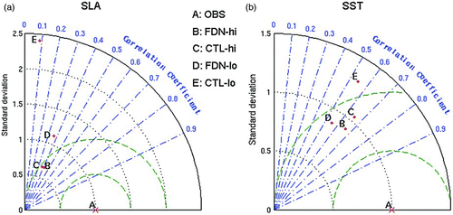
A Taylor diagram for sea surface temperature (Fig. 12b, note change in scale) has also been constructed using the gridded CMC sea surface temperature fields as observations (see Section 3 for a description of this dataset). The results for the high frequency variations of the control and nudged runs are similar (points B and C): the standard deviations of the simulations are close to 1; the correlation with observations is about 0.65; and the standard deviation of the errors is about 0.8. At low frequency the nudged run (point D) outperforms the control run (point E) in terms of standard deviation of the simulations (0.8 versus 1.3) and standard deviation of the errors (0.9 versus 1.2); the correlation with the observations is quite similar for both runs (0.55). Overall the results for surface temperature are qualitatively similar to those for sea level although the better performance of the nudged run is not as pronounced. We note that the CMC sea surface temperature observations were used in the generation of the GEM atmospheric fields (Smith et al., 2013) used to force both models. This may explain why the standard deviations of the simulations are closer to observations. The correlations for sea surface temperature are higher and simulation errors lower than for sea level.

6 Summary and discussion

Frequency-dependent nudging has been used to suppress the drift and bias of a coarse resolution (1°) global ocean model. The idea is to nudge the model toward an observed seasonal climatology in frequency bands that are centred on frequencies resolved by the climatology. In the present study we nudged temperature and salinity to the central frequencies of 0 and 1 cycles per year. The width of the frequency bands over which nudging occurred was 1/3 cycle per year; outside these bands the model was not nudged.

It was first shown that the version of the global ocean model that was not nudged exhibited significant drift and bias. The long-term mean temperature was shown to be too warm over much of the global ocean, and the long-term mean salinity also showed large-scale biases of almost 1 over much of the global ocean. The long-term surface circulation of the model that was not nudged was also shown to be unrealistic in the Gulf Stream and the Kuroshio Extension. Bias errors were also found for the annual cycle; in particular the simulated surface salinity averaged over the North Atlantic was out of phase with the observed annual cycle.

Frequency-dependent nudging was shown to significantly reduce most of the biases in temperature, salinity, sea level, and surface flow described in the preceding paragraph. This is consistent with the performance of frequency-dependent nudging found in earlier regional studies using higher resolution, eddy-permitting models (e.g., Wright et al. (2006) for the North Atlantic and Stacey et al. (2006) for the North Pacific).

We next examined the variability about the annual cycle. Visual examination of observed and predicted time series and their cross spectral analysis (not shown) led us to consider the variability in two frequency bands: low frequency (periods longer than 1 year) and high frequency (periods shorter than 1 year). We focused primarily on sea level, mainly because of its practical and scientific relevance but also because it is a completely independent dataset in terms of model validation.

Frequency-dependent nudging had a relatively small impact on the standard deviation of the high frequency sea level simulations; the standard deviations of the control and nudged runs were quite similar. Both runs failed to reproduce high standard deviations in regions of strong, unstable currents (e.g., Gulf Stream and Kuroshio Extension). This is not surprising given the coarse resolution of the ocean model. We were encouraged to find, however, that nudging did increase the correlation between the observed and simulated sea level in the equatorial Pacific and Atlantic oceans. We attribute this to the model's more realistic background state that was maintained by the frequency-dependent nudging. Frequency-dependent nudging had a much more significant impact on the simulations of sea level at low frequency. The nudging effectively eliminated model drift leading to more realistic maps of the standard deviation of low frequency sea level and higher correlations between low frequency changes of observed and simulated sea level.

Frequency-dependent nudging requires a realistic seasonal climatology toward which the model is to be nudged. This means that frequency-dependent nudging is not suitable for use in climate studies where the future seasonal climate is to be determined. Although frequency-dependent nudging can allow the annual cycle to vary from year to year, it will generally suppress variability at low frequency and at frequencies close to one cycle per year (e.g., variability associated with the Pacific Decadal Oscillation and El Niño). The amount of suppression can be reduced by decreasing the κ parameter in the frequency-dependent filter (Thompson et al., 2006), but this will increase the spin-up time of the model, which is proportional to κ⁻¹. In terms of short-term ocean or coupled atmosphere–ocean forecasting, an accurate up-to-date seasonal climatology is essential.

With regard to future work, we plan to apply frequency-dependent nudging to a higher resolution ocean model coupled to an atmospheric forecast model as part of the ongoing effort to build an operational coupled forecast system for Canada. It is expected that the nudging will significantly improve the system's performance by suppressing ocean model drift and bias, hence, improving the air–sea fluxes. We expect it will also improve short-term forecasts by minimizing initialization shocks caused by the assimilation of observations into a biased model. Frequency-dependent nudging and data assimilation will act in two different ways to restore the model to the observations. Frequency-dependent nudging will reduce model biases, and data assimilation will refine the initial state for the forecast. It will be essential that the observed climatology to which the model is nudged be consistent with the observations although, as noted earlier, the frequency-dependent filter can allow for some interannual variability in both the mean and annual cycles. We will be particularly interested in quantifying the impact of frequency-dependent nudging on the forecast skill at medium to long ranges. It is possible that the benefits of frequency-dependent nudging will be more evident in a higher resolution ocean model than the one considered here because it will lead to a more realistic representation of processes such as baroclinic instability that draw their energy from the background state.

Acknowledgements

We first thank our friend and colleague Dr. Daniel G. Wright for writing the frequency-dependent nudging code used in this study. Without his contributions and encouragement this study would not have been completed. We are grateful to the Canadian Foundation for Climate and Atmospheric Sciences and the Marine Environmental Observation and Response Network (MEOPAR) of Centres of Excellence for support. We also thank François Roy and Eric Oliver for programming support, Gregory Smith for providing free access to his meteorological dataset (Smith et al., 2013), and Fred Woslyng for assistance preparing the figures.

References

- Balmaseda, M. A. (2004). Ocean data assimilation for seasonal forecasts. In ECMWF Seminar Proceedings. Seminar on recent developments in data assimilation for atmosphere and ocean (pp. 301–326). Reading, UK, 8–12 September 2003.
- Balmaseda, M. A., Dee, D., Vidard, A., & Anderson, D. L. T. (2007). A multivariate treatment of bias for sequential data assimilation: Application to the tropical oceans. Quarterly Journal of the Royal Meteorological Society, 133(622), 167–179. doi: 10.1002/qj.12
- Barnier, B., Madec, G., Penduff, T., Molines, J.-M., Treguier, A.-M., Le Sommer, J., … De Cuevas, B. (2006). Impact of partial steps and momentum advection schemes in a global ocean circulation model at eddy permitting resolution. Ocean Dynamics, 56, 543–567. doi:10.1007/s10236-006-0082-1
- Bleck, R. (2002). An oceanic general circulation model framed in hybrid isopycnic-Cartesian coordinates. Ocean Modelling, 4(1), 55–88. doi: 10.1016/S1463-5003(01)00012-9
- Bonjean, F. (2001). Influence of surface currents on the sea surface temperature in the tropical Pacific. Journal of Physical Oceanography, 31(4), 943–961. doi: 10.1175/1520-0485(2001)031<0943:IOSCOT>2.0.CO;2
- Brasnett, B. (2008). The impact of satellite retrievals in a global sea-surface-temperature analysis. Quarterly Journal of the Royal Meteorological Society, 134(636), 1745–1760. doi: 10.1002/qj.319
- Chepurin, G. A., Carton, J. A., & Dee, D. (2005). Forecast model bias correction in ocean data assimilation. Monthly Weather Review, 133(5), 1328–1342. doi: 10.1175/MWR2920.1
- Côté, J., Gravel, S., Méthot, A., Patoine, A., Roch, M., & Staniforth, A. (1998). The operational CMC-MRB Global Environmental Mulitscale (GEM) model. Part I: Design considerations and formulation. Monthly Weather Review, 126(6), 1373–1395. doi: 10.1175/1520-0493(1998)126<1373:TOCMGE>2.0.CO;2
- D'Andrea, F., & Vautard, R. (2000). Reducing systematic errors by empirically correcting model errors. Tellus A, 52(1), 21–41. doi: 10.1034/j.1600-0870.2000.520103.x
- Dee, D. P. (2005). Bias and data assimilation. Quarterly Journal of the Royal Meteorological Society, 131(613), 3323–3343. doi: 10.1256/qj.05.137
- Dee, D. P., & da Silva, A. M. (1998). Data assimilation in the presence of forecast bias. Quarterly Journal of the Royal Meteorological Society, 124(545), 269–295. doi: 10.1002/qj.49712454512
- Delcroix, T., & Picaut, J. (1998). Zonal displacement of the western equatorial Pacific fresh pool. Journal of Geophysical Research, 103(C1), 1087–1098. doi: 10.1029/97JC01912
- Ducet, N., Le Traon, P. Y., & Reverdin, G. (2000). Global high-resolution mapping of ocean circulation from the combination of T/P and ERS-1/2. Journal of Geophysical Research, 105(C8), 19477–19498. doi: 10.1029/2000JC900063
- Fichefet, T., & Morales Maqueda, M. A. (1997). Sensitivity of a global sea ice model to the treatment of ice thermodynamics and dynamics. Journal of Geophysical Research, 102(C6), 12609–12646. doi: 10.1029/97JC00480
- Griffith, A. K., & Nichols, N. K. (1996). Accounting for model error in data assimilation using adjoint methods. In M. Berz, C. Bischof, G. Corliss, & A. Griewank (Eds.), Computational differentiation: Techniques, applications, and tools (pp. 195–204). Santa Fe, New Mexico: SIAM, Society for Industrial and Applied Mathematics.
- Griffith, A. K., & Nichols, N. K. (2000). Adjoint methods in data assimilation for estimating model error. Flow Turbulence and Combustion, 65, 469–488. doi: 10.1023/A:1011454109203
- Guilyardi, E., Gualdi, S., Slingo, J., Navarra, A., Delecluse, P., Cole, J., … Terray, L. (2004). Representing El Niño in coupled ocean–atmosphere GCMs: The dominant role of the atmospheric component. Journal of Climate, 17(24), 4623–4629. doi: 10.1175/JCLI-3260.1
- Halliwell, G. R. (2004). Evaluation of vertical coordinate and vertical mixing algorithms in the HYbrid-Coordinate Ocean Model HYCOM. Ocean Modelling, 7(3), 285–322. doi: 10.1016/j.ocemod.2003.10.002
- Huddleston, M. R., Bell, M. J., Martin, M. J., & Nichols, N. K. (2004). Assessment of wind-stress errors using bias corrected ocean data assimilation. Quarterly Journal of the Royal Meteorological Society, 130(598), 853–871. doi: 10.1256/qj.02.213
- Kamen, E. W., & Su, J. K. (1999). Introduction to optimal estimation. London, UK: Springer.
- Large, W., & Yeager, S. (2004). Diurnal to decadal global forcing for ocean and sea-ice models: The data sets and flux climatologies. NCAR Technical Note: NCAR/TN-460+STR. Boulder, CO: CGD Division of the National Center for Atmospheric Research.
- Large, W. G., & Yeager, S. G. (2009). The global climatology of an interannually varying air–sea flux data set. Climate Dynamics, 33(2-3), 341–364. doi: 10.1007/s00382-008-0441-3
- Latif, M., Barnett, T. P., Cane, M. A., Flugel, M., Graham, N. E., Von Storch, H., … Zebiak, S. E. (1994). A review of ENSO prediction studies. Climate Dynamics, 9(4-5), 167–179. doi: 10.1007/BF00208250
- Levitus, S. (1998). Climatological atlas of the world ocean. NOAA Prof. Paper 13.
- Lin, J.-L. (2007). Interdecadal variability of ENSO in 21 IPCC AR4 coupled GCMs. Geophysical Research Letters, 34(12), L12702. doi:10.1029/2006GL028937
- Lu, Y., Wright, D. G., & Yashayaev, I. (2007). Modelling hydrographic changes in the Labrador sea over the past five decades. Progress in Oceanography, 73(3), 406–426. doi: 10.1016/j.pocean.2007.02.007
- Madec, G., Delecluse, P., Imbard, M., & Levy, C. (1998). OPA8.1 Ocean general Circulation Model reference manual. Notes du Pôle de Modélisation, Institut Pierre Simon Laplace (IPSL), France, no. 11.
- Maltrud, M. E., & McClean, J. L. (2005). An eddy resolving global 1/10 ocean simulation. Ocean Modelling, 8(1-2), 31–54. doi: 10.1016/j.ocemod.2003.12.001
- van Oldenborgh, G. J., Philip, S. Y., & Collins, M. (2005). El Niño in a changing climate: A multi-model study. Ocean Science, 1, 81–95. doi: 10.5194/os-1-81-2005
- Picaut, J., Ioualalen, M., Menkes, C., Delcroix, T., & McPhaden, M. J. (1996). Mechanism of the zonal displacements of the Pacific warm pool: Implications for ENSO. Science, 274, 1486–1489. doi: 10.1126/science.274.5292.1486
- Pierce, D. W. (1996). Reducing phase and amplitude errors in restoring boundary conditions. Journal of Physical Oceanography, 26(8), 1552–1560. doi: 10.1175/1520-0485(1996)026<1552:RPAAEI>2.0.CO;2
- Rasmusson, E. M., & Carpenter, T. H. (1982). Variations in tropical sea surface temperature and surface wind fields associated with the southern oscillation/El Niño. Monthly Weather Review, 110(5), 354–384. doi: 10.1175/1520-0493(1982)110<0354:VITSST>2.0.CO;2
- Segschneider, J., Balmaseda, M. A., & Anderson, D. L. T. (2000). Anomalous temperature and salinity variations in the tropical Atlantic: Possible causes and implications for the use of altimeter data. Geophysical Research Letters, 17(15), 2281–2284. doi: 10.1029/1999GL011310
- Smith, G., Roy, F., Mann, P., Dupont, F., Brasnett, B., Lemieux, J-F., … Blair, S. (2013). A new atmospheric data set for forcing ice-ocean models: Evaluation of CMC GDPS reforecasts. Quarterly Journal of the Royal Meteorological Society, 140(680), 881–894. doi: 10.1002/qj.2194
- Stacey, M. W., Shore, J., Wright, D. G., & Thompson, K. R. (2006). Modeling events of sea-surface variability using spectral nudging in an eddy permitting model of the northeast Pacific Ocean. Journal of Geophysical Research, 111(C6), C06037. doi:10.1029/2005JC003278
- Taylor, K. E. (2001). Summarizing multiple aspects of model performance in a single diagram. Journal of Geophysical Research, 106(D7), 7183–7192. doi: 10.1029/2000JD900719
- Thiebaux, H. J., & Morone, L. L. (1990). Short-term systematic errors in global forecasts: Their estimation and removal. Tellus A, 42(2), 209–229. doi: 10.1034/j.1600-0870.1990.00001.x
- Thompson, K. R., Wright, D. G., Lu, Y., & Demirov, E. (2006). A simple method for reducing seasonal bias and drift in eddy resolving ocean models. Ocean Modelling, 13(2), 109–125. doi: 10.1016/j.ocemod.2005.11.003
- Vidard, A., Anderson, D. L. T., & Balmaseda, M. A. (2007). Impact of ocean observation systems on ocean analysis and seasonal forecasts. Monthly Weather Review, 135(2), 409–429. doi: 10.1175/MWR3310.1
- Wright, D. G., Thompson, K. R., & Lu, Y. (2006). Assimilating long-term hydrographic information into an eddy-permitting model of the North Atlantic. Journal of Geophysical Research, 111(C9), C09022. doi:10.1029/2005JC003200
- Zhu, J., Demirov, E., Dupont, F., & Wright, D. (2010). Eddy-permitting simulations of the sub-polar North Atlantic: Impact of the model bias on water mass properties and circulation. Ocean Dynamics, 60(C9), 1177–1192. doi: 10.1007/s10236-010-0320-4