Simulations of Boreal Summer Intraseasonal Oscillations with the Climate Forecast System, version 2, over India and the Western Pacific: Role of Air–Sea Coupling

Abstract

In this study, we examine the characteristics of the boreal summer monsoon intraseasonal oscillation (BSISO) using the second version of the Climate Forecast System (CFSv2) and revisit the role of air–sea coupling in BSISO simulations. In particular, simulations of the BSISO in two carefully designed model experiments are compared: a fully coupled run and an uncoupled atmospheric general circulation model (AGCM) run with prescribed sea surface temperatures (SSTs). In these experiments an identical AGCM is used, and the daily mean SSTs from the coupled run are prescribed as a boundary condition in the AGCM run. Comparisons indicate that air–sea coupling plays an important role in realistically simulating the BSISO in CFSv2. Compared with the AGCM run, the coupled run not only simulates the spatial distributions of intraseasonal rainfall variations better but also shows more realistic spectral peaks and northward and eastward propagation features of the BSISO over India and the western Pacific. This study indicates that including an air–sea feedback mechanism may have the potential to improve the realism of the mean flow and intraseasonal variability in the Indian and western Pacific monsoon region.

Résumé

[Traduit par la rédaction] Dans cette étude, nous examinons les caractéristiques de l'oscillation intrasaisonnière de la mousson d’été boréal (BSISO) à l'aide de la seconde version du CFDv2 (Climate Forecast System) et nous revisitons le rôle du couplage air-mer dans les simulations BSISO. En particulier, nous comparons les simulations du BSISO dans deux expériences par modèle soigneusement élaborées : une passe couplée complète et une passe du modèle de circulation générale atmosphérique (AGCM) non couplée avec des températures de surface de la mer prescrites. Dans ces expériences, nous utilisons un AGCM identique et les températures moyennes journalières de la surface de la mer utilisées dans la passe couplée sont prescrites comme une condition aux limites dans la passe de l'AGCM. Les comparaisons indiquent que le couplage air–mer joue un rôle important en simulant de façon réaliste la BSISO dans le CFSv2. Comparativement à la passe AGCM, la passe couplée non seulement simule mieux les distributions spatiales des variations des chutes de pluie intrasaisonnières mais aussi montre des pics spectraux et des caractéristiques de propagation vers le nord et vers l'est plus réalistes de la BSISO en Inde et dans l'ouest du Pacifique. Cette étude indique que l'inclusion d'un mécanisme de rétroaction air–mer peut permettre d'accroître le réalisme de l’écoulement moyen et de la variabilité intrasaisonnière dans la région de la mousson en Inde et dans l'ouest du Pacifique.

Keywords:

• intraseasonal oscillation
• summer monsoon
• air–sea coupling
• Climate Forecast System version 2

1 Introduction

The boreal summer intraseasonal oscillation (BSISO) has a more complex spatial structure and propagation than the winter Madden–Julian Oscillation (MJO), and its eastward propagation is often accompanied by northward propagation over the Indian Ocean and western Pacific region (Shukla, 2014). On an intraseasonal scale, it is characterized by active and break phases of the Asian summer monsoon system, and its northward propagation plays a vital role in the onset, withdrawal, and intraseasonal variability of the Indian summer monsoon, and the mei-yu regime over south China (Annamalai & Slingo, 2001; Goswami, 2005 among others; Krishnamurti & Subrahmanyam, 1982; Yasunari, 1979), which affects more than 60% of the world's population. Thus, accurate simulations and predictions of the BSISO are highly desirable.

Nowadays, simulating the space–time characteristics of the BSISO still remains a big challenge for state-of-the-art climate models. By analyzing model output from the Coupled Model Intercomparison Project, phase 3 (CMIP3), Sperber and Annamalai (2008) demonstrated that only a few models produce the tilted structure of convection variability that extends from India to the Maritime Continent. Lin et al. (2008) also found that most CMIP3 models display too red a spectrum in precipitation in the 12–24 day frequency bands. Although some CMIP3 models exhibited northward propagation of the intraseasonal convective anomalies (Lin et al., 2008), only a few simulated the northward propagation that occurs in conjunction with the eastward propagation of near-equatorial convection (Sperber & Annamalai, 2008). Most of the latest CMIP5 models also failed to simulate realistic equatorial eastward propagation beyond the Maritime Continent and also underestimated the BSISO variance, even though more of the models in CMIP5 simulated the northward propagation of BSISO than in CMIP3 (Sabeerali et al., 2013).

On the other hand, the improved simulation of the BSISO by coupled models over stand-alone atmospheric general circulation models (AGCMs) suggests that air–sea coupling has an effect on BSISO (Achuthavarier & Krishnamurthy, 2011; Fu, Wang, Li, & McCreary, 2003; Fu, Wang, Waliser, & Tao, 2007; Kemball-Cook, Wang, & Fu, 2002; Rajendran, Kitoh, & Arakawa, 2004; Sharmila et al., 2013; Wang, Chen, & Kumar, 2009) in addition to atmospheric dynamics (Wang, 2005). As shown by observations (Vecchi & Harrison, 2002), systematic changes in sea surface temperature (SST) over the Bay of Bengal occur in conjunction with the northward propagation of intraseasonal convection, which suggests that air–sea interaction might be an important feature in the propagation of the BSISO (note that observational studies cannot eliminate the possibility that intraseasonal SST variability is following atmospheric forcing). Using a hybrid atmosphere–ocean coupled model, Fu et al. (2003) suggested that air–sea coupling is the most important process associated with the eastward and northward propagation of the BSISO for promoting the proper propagation feature, and their later study (Fu et al., 2007) further investigated the effect of coupling on the predictability of the BSISO. The impact of air–sea coupling over the Indian Ocean on the BSISO was also emphasized by Rajendran et al. (2004) using the CGCM from the Meteorological Research Institute (MRI) of the Japan Meteorological Agency (JMA). DeMott, Stan, Randall, Kinter, and Khairoutdinov (2011) and Meehl et al. (2012) compared two fully coupled AOGCM simulations with corresponding simulations from the Atmospheric Model Intercomparison Project (AMIP) forced by observed SSTs in the Asian–Australian monsoon region. They also found that coupled experiments improved some aspects of monsoon simulations, even though the coupling factor cannot be isolated from the influence of different SSTs.

However, not all coupled systems capture the effect of air–sea coupling in simulating the BSISO, especially fully coupled AOGCMs. Seo, Schemm, Wang, and Kumar (2007), using version 1 of the Climate Forecast System (CFSv1), found that coupling showed only limited improvements in simulations of the BSISO, unless the cold bias in the Indian Ocean was corrected with a flux adjustment to the ocean surface flux components. Also, with a hybrid atmosphere–ocean coupled model, Kemball-Cook et al. (2002) found that the coupled run simulated the intraseasonal oscillation in winter and May–June better than the uncoupled run, but its performance degraded in August–October, which they attributed to the absence of an easterly vertical shear in the mean zonal wind in the basic state of the coupled model. Also, Kim and Kang (2008), using the coupled general circulation model from Soeul National University, found similar results from the CGCM and AGCM runs in terms of both the BSISO simulation characteristics and its predictability. In Meehl et al. (2012), it was found that the intraseasonal variability in the Community Climate System Model, version 4 (CCSM4), is similar to that in its atmospheric component, the Community Atmosphere Model, version 4 (CAM4), in spite of the different mean states and ocean coupling in CCSM4 that do not significantly affect the simulation of this variability in either the Indian or western Pacific regions.

In this study, we examine BSISO characteristics in the second version of the Climate Forecast System (CFSv2) and re-visit the effect of air–sea coupling in the simulations of the BSISO. The work is a continuation of Zhu and Shukla (2013) in which the role of air–sea coupling in the seasonal prediction of Asia–Pacific summer monsoon rainfall was quantified using CFSv2, but in this study the intraseasonal variability over the same region is the focus. Our study of the BSISO covers the entire Indian and western Pacific region, and its propagation in both the zonal and meridional directions will be examined. To isolate the role of air–sea coupling from other factors, in our experiments the identical AGCM (Global Forecast System (GFS)) is used in both the CGCM and AGCM runs, and daily mean SSTs from the CGCM run are used as boundary conditions in the AGCM run. It will be shown that in CFSv2 the air–sea feedback significantly improves simulation of the BSISO, including its propagation features over India and the western Pacific region and its spectral peaks. The next section describes the model, the experimental design, the verification dataset, and the analysis method. The results are presented in Section 3. Concluding remarks are made in Section 4.

2 Model descriptions, experimental design, and datasets

The coupled model used in this study is the CFSv2 (Saha et al., 2014) from the National Centers for Environmental Prediction (NCEP), which consists of the NCEP GFS at T126 horizontal resolution (105 km grid spacing) with 64 vertical levels in a hybrid sigma-pressure coordinate. The ocean model is the Geophysical Fluid Dynamics Laboratory (GFDL) Modular Ocean Model (MOM), version 4.0, which is configured for the global ocean with a horizontal grid of 0.5° × 0.5° poleward of 30°S and 30°N and a meridional resolution that gradually increases to 0.25° between 10°S and 10°N. The vertical coordinate is geopotential (z-) with 40 levels (27 of them in the upper 400 m). The maximum depth is approximately 4.5 km. The oceanic and atmospheric components exchange surface momentum, heat, and freshwater fluxes every 30 minutes. More information on CFSv2 can be found in Saha et al. (2014). A recent analysis of simulations of the BSISO indicates that CFSv2 is among the best at simulating the BSISO when compared with state-of-the-art CMIP5 models (Sabeerali et al., 2013).

In this study, two groups of experiments are analyzed: a CGCM run and an AGCM run in which an identical AGCM (GFS) is used. In the CGCM run, the ocean initial conditions (OICs) are from the European Centre for Medium range Weather Forecasts (ECMWF) Ocean Reanalysis System 4 (ORAS4; Balmaseda, Mogensen, & Weaver, 2013), which takes into account the substantial difference among different ocean analyses (Zhu, Huang, & Balmaseda, 2012a), and CFSv2 produces better predictions of SSTs especially in the eastern Pacific when using ORAS4 OICs (Zhu et al., 2012b). For each OIC, runs with four members are conducted for each year from 1982 to 2009 differing in their atmospheric and land initial conditions, which are the instantaneous fields from 00:00 utc of the first four days of April each year in the NCEP Climate Forecast System Reanalysis (CFSR; Saha et al., 2010). In the AGCM run, the daily mean SSTs from the CGCM run (CFSv2) are prescribed as boundary conditions, and the atmospheric and land initial conditions are the same as in the CGCM run, which means that the only difference between the two runs is the coupling in the CGCM run.

In this study, the outputs from the CGCM and AGCM from 1 June to 30 September (122 days) each year are used to examine the simulations of the BSISO. Discarding the first two months of each simulation ensures that there is little effect on the intraseasonal signals from the initial conditions so the difference between the CGCM and AGCM runs mainly comes from the coupling in the CGCM run. During the analysis process, the CGCM and AGCM outputs are first bi-linearly interpolated onto a 1° × 1° grid from the observational verification precipitation data, the Global Precipitation Climatology Project (GPCP) daily gridded precipitation (Huffman et al., 2001). The GPCP precipitation data from 1997 to 2009 are used in the study. For both observations and model simulations, daily anomalies are obtained by subtracting their respective seasonally varying climatological means, and the internannual variations are removed by further subtracting the mean for each year. An empirical orthogonal function (EOF) analysis is applied over the Indian and western Pacific (IWP) domain (57.5°E–180°E, 22.5°S–40°N) as in Shukla (2014), based on the daily fields from 1997 to 2009 (13 years), the common period between the GPCP daily data and model simulations. For model simulations, four individual members of each year are combined; for the 13 years analyzed this gives 52 members of the June, July, August, and September (JJAS) simulation. The following discussion is based on the analysis of the 52 members, unless indicated otherwise. However, an analysis using one member of each year yields similar results. In addition, similar analyses were also conducted based on all the years (1982–2009) for the CGCM and AGCM runs, and results similar to those for the 13 years were obtained (results not shown).

The observation-based monthly SST analysis from the optimum interpolation analysis, version 2 (OIv2) SST dataset (Reynolds, Rayner, Smith, Stokes, & Wang, 2002) is also used to examine the SST biases in CFSv2.

3 Results

As identified in Zhu and Shukla (2013), both the CGCM and AGCM runs generally capture the observed rainfall distributions, but the AGCM produces higher rainfall biases (see also Figs 1a, 1b, and 1c) and unrealistically high interannual variations in rainfall in the tropical western North Pacific (TWNP; 110°E–165°E, 5°N–20°N) region and west of the Philippines compared with the CGCM run. Similar to the interannual variability, the intraseasonal rainfall variations from AGCM (Fig. 1f) are also clearly larger than those from CGCM (Fig. 1e) over similar regions, with the latter closer to those in the GPCP rainfall (Fig. 1d). Figure 2 depicts the coefficients of variation (CV) in rainfall for both observations and model simulations; CV is defined as the ratio of the daily standard deviation to the mean. It is observed that the CV distributions for the CGCM (Fig. 2b) and AGCM (Fig. 2c) runs are similar and only slightly different from the GPCP observations (Fig. 2a). This suggests that the difference in intraseasonal rainfall variations between the AGCM and CGCM runs is possibly due to the difference in their rainfall climatology. It is likely that by modifying the rainfall climatological distribution the coupling acts as an important “damping” force on an intraseasonal time scale in regions like the TWNP and west of the Phillippines.

Fig. 1 The climatology of JJAS rainfall is shown in (a) GPCP observations, (b) CGCM, and (c) AGCM. Standard deviation of JJAS daily rainfall anomalies are shown in (d) GPCP observations, (e) CGCM, and (f) AGCM.

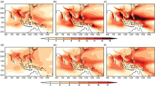
Fig. 2 The coefficients of variation in rainfall defined as the ratio of the daily standard deviation (Figs 1d–1f) to the mean (Figs 1a–1c) in (a) GPCP observations, (b) CGCM, and (c) AGCM.

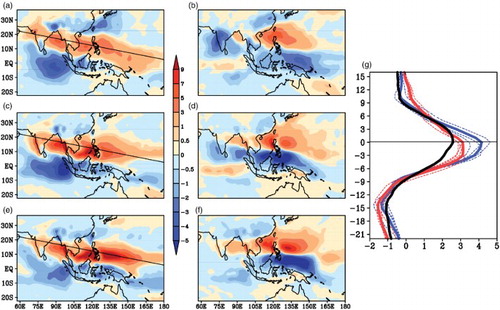
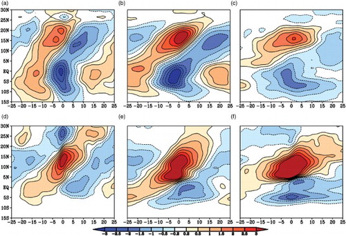
The EOF analysis of daily rainfall anomalies was carried out for the summer monsoon season, with the two leading modes, EOF1 and EOF2, of the GPCP observations, CGCM, and AGCM shown in Figs 3a to 3f. The two modes together explain 6.22, 6.41, and 7.38% of the variance in GPCP, CGCM, and AGCM, respectively. The two leading patterns of the GPCP observations (Figs 3a and 3b) exhibit banded structures with a west-northwest to east-southeast orientation extending from the Arabian Sea eastward to the seas north of New Guinea. The amplitudes of the rainfall perturbations at the major centres of action of EOF1 and EOF2 range up to 5 mm d⁻¹ per standard deviation of the respective (standardized) principal components (PC1 and PC2). In general, in terms of both amplitude and spatial distribution, the CGCM captures the two leading modes relatively well (Figs 3c and 3d versus Figs 3a and 3b). On close inspection, it can be seen that the amplitude of the CGCM EOF1 (Fig. 3c) is slightly higher over the Bay of Bengal and the South China Sea, and the EOF2 pattern (Fig. 3d) has the opposite sign over some parts of central India. The biases in the AGCM are clearly more severe than those in the CGCM. In particular, the amplitude of the rainfall variations in EOF1 (Fig. 3e) over the TWNP region is unrealistically higher than that of GPCP and CGCM, which is consistent with Fig. 1f, and the magnitude is also clearly lower over the central Indian Ocean. The difference in both regions is again possibly related to the rainfall mean difference between AGCM and CGCM. Furthermore, larger biases are present in EOF2 of the AGCM run (Fig. 3f), which presents an unrealistic north–south contrast and is unable to capture many important features in the GPCP observations (Fig. 3b). For example, anomalies of a wrong sign are present over the Bay of Bengal, India, and over some parts of the Arabian Sea. The AGCM is also not able to reproduce the major centre of action over the central Indian Ocean and, as like EOF1, the EOF2 amplitude is unrealistically higher than the GPCP observations and CGCM over the TWNP region. Figure 3g shows the meridional profiles of rainfall in the EOF1 for the GPCP observations, CGCM, and AGCM, which are averaged over the entire width of our domain (57.5°E–180°E) along a set of tilted axes parallel to the reference line as shown in Figs 3a, 3c, and 3e. Similar meridional profiles for the observations are also discussed for various variables in Shukla (2014). It is clearly seen that over the most active region, the CGCM meridional profile is closer to the GPCP counterpart than the AGCM.

Fig. 3 (a), (c), and (e) EOF1 and (b), (d), and (f) EOF2 for rainfall anomalies (mm d⁻¹) based on daily data for June–September in (a), (b) GPCP observations, (c), (d) CGCM, and (e), (f) AGCM. The black lines in (a), (c), and (e) denote the location of action centre associated with the maximum rainfall and is the reference line for (g). (g) Meridional profiles of rainfall in the EOF1 mode of GPCP, CGCM, and AGCM averaged along a set of tilted axes parallel to the reference line in (a), (c), and (e); the black, red, and blue curves indicate the GPCP observations, CGCM, and AGCM, respectively. For the CGCM and AGCM curves, the solid (dotted) lines are based on the entire 52-member JJAS data (four members each with 13-year JJAS data). The y-axis in (g) denotes the latitude relative to the reference line.

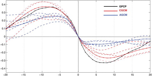
Meanwhile, in both the GPCP observations and CGCM there seems to be a connection between EOF1 and EOF2, with EOF2 being displaced northward relative to EOF1, which, however, is not clear in the AGCM. There is actually a tendency for EOF1 to evolve into EOF2 over the course of approximately one week, which is evidenced by a maximum correlation of 0.35 (0.36) when PC1 leads PC2 by approximately seven days (approximately nine days) in the GPCP observations (CGCM) (see Fig. 3). Also from Fig. 4, it is clearly shown that the lack of coupling systematically degrades the relationship when PC1 lags PC2. In particular, AGCM reproduces a significantly weaker relationship when an EOF2 leads a negative EOF1, which achieves a maximum correlation of approximately 0.1 at approximately two days, in contrast to 0.32 at approximately eight days in the GPCP. On the other hand, CGCM captures the lagged relationship remarkably well, which has a maximum correlation of 0.28 at a similar time delay.

Fig. 4 Lead-lag correlation between PC1 and PC2. A lag of −1 indicates that PC1 leads PC2 by 1 day. The black, red, and blue lines indicate the GPCP observations, CGCM, and AGCM runs, respectively. For the CGCM and AGCM curves, the solid lines are based on the entire 52-member JJAS data; the dashed lines represent the four members, each with 13-year JJAS data.

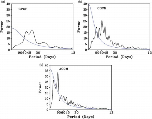
In addition to the degraded performance in simulating rainfall distributions, AGCM also degrades the simulated intraseasonal frequencies. Figure 5 shows the power spectra of PC1s for the GPCP observations, CGCM, and AGCM. In the CGCM run (Fig. 5b), the spectrum is characterized by major peaks between 30 and 60 days, which is consistent with the spectrum of PC1 in the GPCP (Fig. 5a). The bulk power of PC1 in the GPCP observations and CGCM is concentrated at intraseasonal periods (i.e., 30–60 days) typically associated with the BSISO. However, the PC1 for AGCM (Fig. 5c) shows a power spectrum peak at a time period longer than 90 days. Similar degraded simulations by AGCM are also shown in the spectral analysis of PC2 (not shown here).

Fig. 5 Power spectra of the rainfall PC1 in (a) GPCP observations, (b) CGCM, and (c) AGCM. The dashed blue curve is the 95% confidence level of a red noise test.

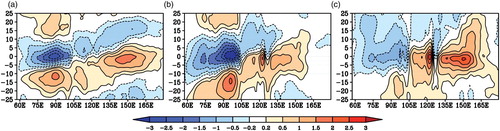
Figures 6a, 6b, and 6c are the Hovmöller diagrams of rainfall anomalies averaged over 70°E–90°E (the Indian subcontinent) regressed onto the normalized PC1 in the GPCP, CGCM, and AGCM, respectively. In GPCP (Fig. 6a), a well-defined northward-propagating rainfall band from 5°S (the Indian Ocean) to 25°N (continental India) is clearly observed. This feature is captured well by the CGCM (Fig. 6b), even though the speed of the northward propagating band in CGCM is slightly slower than in the GPCP observations. On the other hand, rainfall in the AGCM is mostly stationary with weak propagating signals, which reflects the role of atmospheric dynamics in the BSISO (Wang, 2005). The improvement in northward propagation over this region with coupling is also discussed by Sharmila et al. (2013). Further, the same difference is also exhibited for the BSISO in the western Pacific region (Figs 6d, 6e, and 6f). As shown in Fig. 6d, there are well-defined northward propagating rainfall bands from 5°S to 30°N in the GPCP observations, which are also captured remarkably well by the CGCM (Fig. 6e). Still, AGCM (Fig. 6f) produces a mostly stationary mode with somewhat less clear and much slower northward propagation. While studies have argued that air–sea interaction is not important for northward propagation over the western Pacific region (Hsu & Weng, 2001), our studies clearly suggest that the presence of air–sea coupling can improve the representation of the northward propagation feature over the region, which might suggest that coupling plays an important role over this region as well.

Fig. 6 Hovmöller plots of rainfall anomalies (mm d⁻¹) averaged over 70°E–90°E (Indian subcontinent) (a), (b), and (c) and 122.5°E–132.5°E (the western Pacific region) (d), (e), and (f) regressed onto the normalized PC1 in (a) and (d) GPCP, (b) and (e) CGCM, and (c) and (f) AGCM.

Further, while most CMIP5 models failed to simulate realistic equatorial eastward propagation beyond the Maritime Continent (Sabeerali et al., 2013), it is encouraging to observe that CFSv2 captures the zonal propagation relatively well. Figures 7a, 7b, and 7c are the Hovmöller diagrams of rainfall anomalies averaged over 10°S–10°N regressed onto the normalized PC1 in GPCP, CGCM, and AGCM. Comparing Fig. 7b with Fig. 7a, it can be seen that the eastward propagation in the CGCM simulation is relatively realistic; it extends from 60°E to 165°E, well beyond the Maritime Continent. In AGCM, the inconsistency with observations is even greater than in the meridional propagations (Fig. 6), which shows almost no propagation.

Fig. 7 Hovmöller plots of rainfall anomalies (mm d⁻¹) averaged over 10°S–10°N regressed onto the normalized PC1 in (a) GPCP observations, (b) CGCM, and (c) AGCM.

4 Conclusions and discussion

The South Asian monsoon exhibits a broad range of variability, and the BSISO is one of the major systems affecting the summer monsoon system in the IWP region. Monsoon prediction by dynamical models is strongly dependent on the ability to simulate the BSISO. In this study, we examined the influence of air–sea coupled processes on the rainfall related to the BSISO over the IWP region. To achieve this, two sets of carefully designed experiments were conducted based on the CFSv2 state-of-the-art coupled system. In these experiments, the same AGCM (i.e., GFS) is used in the coupled and uncoupled runs, and the daily mean SSTs from the coupled run are prescribed as a boundary condition in the uncoupled predictions. Also, the same atmospheric initial conditions are used for both runs. By doing so, the effect of coupling can be identified. The two sets of runs start in April and end in September each year from 1982 to 2009, with four ensemble members each year.

The simulations for the above two sets of runs are compared with the GPCP rainfall observations. It is found that, in the absence of air–sea coupling, AGCM produces more unrealistic features and biases than CGCM. In particular, higher rainfall biases and higher intraseasonal variations in rainfall are shown over the TWNP region. The dominant BSISO rainfall modes in the AGCM simulation are more different than the CGCM simulation compared with the GPCP observations. For example, the AGCM produces stronger rainfall variability in both leading EOFs over the western Pacific region, and its EOF2 has rainfall variations with opposite signs over regions like the Bay of Bengal, the Indian Ocean, and India. Meanwhile, the connection between two modes is also unrealistically low in the AGCM compared with GPCP observations and the CGCM. An EOF2 evolves to a negative EOF1 with a 2-day lag in AGCM with a maximum correlation of approximately 0.1, while the lag is approximately 8 days with a correlation of 0.32 in the GPCP observations. The AGCM also produces an unrealistic spectral power distribution, with a spectrum peak corresponding to oscillations longer than 90 days compared with the 30–60 day period in the observations and in the CGCM. The northeastward propagation features are also simulated less realistically by the AGCM over India and the western Pacific. On the contrary, the above features are captured significantly more realistically by the CGCM.

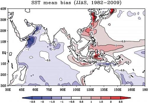
These comparisons indicate that coupling may be an important factor for simulating intraseasonal rainfall variability in the Indian and western Pacific monsoon region, thus coupled atmosphere–ocean models are more promising tools for predicting climate over the region at intraseasonal to seasonal time scales. However, it should be noted that our findings might be model dependent. In fact, it is possible that the SST errors could distort the role of air–sea interactions at sub-seasonal temporal scales. For example, Klingaman and Woolnough (2014) recently demonstrated that mean-state errors could lead to a false impression of the role of coupling; in that study, the mean-state SST biases in the Hadley Centre coupled model damped the MJO. As in some studies (DeMott et al., 2011; Meehl et al., 2012), it is hard to isolate the effect of air–sea interactions from those due to different SSTs from a comparison between coupled simulations and AMIP-type simulations forced by observed SSTs. In our experiments, we tried to isolate the coupling factor by using the same SSTs. On the other hand, as shown in Fig. 8, there are clear biases in CFSv2 during the summer monsoon season, including a 0.5°–1°C cold bias in the Arabian Sea and Indian Ocean and a 0.5°–1°C warm bias in the western Pacific sector. It is not easy to explore how SST biases affect our findings of the role of coupling on BSISOs because it is a challenge to eliminate such SST biases in a coupled system. However, we urge that more studies be conducted with similar comparisons based on different state-of-the-art systems to confirm our findings.

Fig. 8 SST mean bias (°C) in CFSv2 relative to OIv2 observations during the summer monsoon season (JJAS) of 1982–2009.

Acknowledgements

Funding for this study was provided by grants from the NSF (ATM-0830068 and 0947837), NOAA (NA09OAR4310058), and NASA (NNX09AN50G and NNX09AI84G). The authors thank Drs J. Shukla, J. Kinter, B. Huang, and H. M. Kim for their helpful comments. We also thank Dr. M. A. Balmaseda from ECMWF for providing the ocean initial conditions and L. Marx's help with setting up the experiment. Computing resources provided by the NASA Advanced Supercomputing (NAS) division are also gratefully acknowledged. The authors are grateful to two anonymous reviewers for their constructive comments and suggestions. We acknowledge the excellent editorial effort of Sheila Bourque whose work improved the readability of this paper.

References

- Achuthavarier, D., & Krishnamurthy, V. (2011). Daily modes of South Asian summer monsoon variability in the NCEP Climate Forecast System. Climate Dynamics, 36, 1941–1958.
- Annamalai, H., & Slingo, J. M. (2001). Active/break cycles: Diagnosis of the intraseasonal variability of the Asian Summer Monsoon. Climate Dynamics, 18, 85–102.
- Balmaseda, M. A., Mogensen, K., & Weaver, A. T. (2013). Evaluation of the ECMWF ocean reanalysis system ORAS4. Quarterly Journal of the Royal Meteorological Society, 139, 1132–1161.
- DeMott, C. A., Stan, C., Randall, D. A., Kinter, J. L., & Khairoutdinov, M. (2011). The Asian monsoon in the superparameterized CCSM and its relationship to tropical wave activity. Journal of Climate, 24, 5134–5156.
- Fu, X., Wang, B., Li, T., & McCreary, J. (2003). Coupling between northward-propagating, intraseasonal oscillations and sea surface temperature in the Indian Ocean. Journal of the Atmospheric Sciences, 60, 1733–1753.
- Fu, X., Wang, B., Waliser, D. E., & Tao, L. (2007). Impact of atmosphere-ocean coupling on the predictability of monsoon intraseasonal oscillations. Journal of the Atmospheric Sciences, 64, 157–174.
- Goswami, B. N. (2005). South Asian monsoon. In W. K. M. Lau & D. E. Waliser (Eds.), Intraseasonal variability in the atmosphere-ocean climate system (pp. 19–62). Heidelberg, Germany: Springer.
- Hsu, H.-H., & Weng, C.-H. (2001). Northwestward propagation of the intraseasonal oscillation in the western North Pacific during the boreal summer: Structure and mechanism. Journal of Climate, 14, 3834–3850.
- Huffman, G. J., Adler, R. F., Morrissey, M. M., Bolvin, D. T., Curtis, S., Joyce, R., … Susskind, J. (2001). Global precipitation at one-degree daily resolution from multi-satellite observations. Journal of Hydrometeorology, 2, 36–50.
- Kemball-Cook, S., Wang, B., & Fu, X. (2002). Simulation of the intraseasonal oscillation in the ECHAM-4 model: The impact of coupling with an ocean model. Journal of the Atmospheric Sciences, 59, 1433–1453.
- Kim, H. M., & Kang, I. S. (2008). The impact of ocean-atmosphere coupling on the predictability of boreal summer intraseasonal oscillation. Climate Dynamics, 31, 859–870.
- Klingaman, N. P., & Woolnough, S. J. (2014). The role of air-sea coupling in the simulation of the Madden-Julian oscillation in the Hadley Centre model. Quarterly Journal of the Royal Meteorological Society. doi:10.1002/qj.2295
- Krishnamurti, T. N., & Subrahmanyam, D. (1982). The 30–50 day mode at 850 mb during MONEX. Journal of the Atmospheric Sciences, 39, 2088–2095.
- Lin, J.-L., Weickman, K. M., Kiladis, G. N., Mapes, B. E., Schubert, S. D., Suarez, M. J., … Lee, M.-I. (2008). Subseasonal variability associated with Asian summer monsoon simulated by 14 IPCC AR4 coupled GCMs. Journal of Climate, 21, 4541–4567.
- Meehl, G. A., Arblaster, J. M., Caron, J. M., Annamalai, H., Jochum, M., Chakraborty, A., & Murtugudde, R. (2012). Monsoon regimes and processes in CCSM4. Part I: The Asian–Australian monsoon. Journal of Climate, 25, 2583–2608.
- Rajendran, K., Kitoh, A., & Arakawa, O. (2004). Monsoon low-frequency intraseasonal oscillation and ocean-atmosphere coupling over the Indian Ocean. Geophysical Research Letters, 31, L02210. doi:10.1029/2003GL019031
- Reynolds, R. W., Rayner, N. A., Smith, T. M., Stokes, D. C., & Wang, W. Q. (2002). An improved in situ and satellite SST analysis for climate. Journal of Climate, 15, 1609–1625.
- Sabeerali, C. T., Ramu Dandi, A., Dhakate, A., Salunke, K., Mahapatra, S., & Rao, S. A. (2013). Simulation of boreal summer intraseasonal oscillations in the latest CMIP5 coupled GCMs. Journal of Geophysical Research: Atmospheres, 118, 4401–4420. doi:10.1002/jgrd.50403
- Saha, S., Moorthi, S., Pan, H.-L., Wu, X., Wang, J., Nadiga, S., … Goldberg, M. (2010). The NCEP climate forecast system reanalysis. Bulletin of the American Meteorological Society, 91, 1015–1057.
- Saha, S., Moorthi, S., Wu, X., Wang, J., Nadiga, S., Tripp, P., … Becker, E. (2014). The NCEP Climate Forecast System version 2. Journal of Climate, 27, 2185–2208. doi:10.1175/JCLI-D-12-00823.1
- Seo, K. H., Schemm, J. K. E., Wang, W., & Kumar, A. (2007). The boreal summer intraseasonal oscillation simulated in the NCEP Climate Forecast System: The effect of sea surface temperature. Monthly Weather Review, 135, 1807–1827.
- Sharmila, S., Pillai, P. A., Joseph, S., Roxy, M., Krishna, R. P. M., Chattopadhyay, R., … Goswami, B. N. (2013). Role of ocean-atmosphere interaction on northward propagation of Indian summer Monsoon Intra-Seasonal Oscillations (MISO). Climate Dynamics, 41, 1651–1669. doi:10.1007/s00382-013-1854-1
- Shukla, R. P. (2014). The dominant intraseasonal mode of intraseasonal South Asian summer monsoon. Journal of Geophysical Research: Atmospheres, 119, 635–651. doi:10.1002/2013JD020335
- Sperber, K. R., & Annamalai, H. (2008). Coupled model simulations of boreal summer intraseasonal (30–50 day) variability, Part 1: Systematic errors and caution on use of metrics. Climate Dynamics, 31, 345–372. doi:10.1007/s00382-008-0367-9
- Vecchi, G. A., & Harrison, D. E. (2002). Monsoon breaks and subseasonal sea surface temperature variability in the Bay of Bengal. Journal of Climate, 15, 1485–1493.
- Wang, B. (2005). Theory. In W. K. M. Lau & D. E. Waliser (Eds.), Intraseasonal variability in the atmosphere-ocean climate system (pp. 307–360). Heidelberg, Germany: Springer.
- Wang, W., Chen, M., & Kumar, A. (2009). Impacts of ocean surface on the northward propagation of the boreal summer intraseasonal oscillation in the NCEP climate forecast system. Journal of Climate, 22, 6561–6576.
- Yasunari, T. (1979). Cloudiness fluctuations associated with the northern hemisphere summer monsoon. Journal of the Meteorological Society of Japan, 57, 227–242.
- Zhu, J., Huang, B., & Balmaseda, M. A. (2012a). An ensemble estimation of the variability of upper-ocean heat content over the tropical Atlantic Ocean with multi-ocean reanalysis products. Climate Dynamics, 39, 1001–1020. doi:10.1007/s00382-011-1189-8
- Zhu, J., Huang, B., Marx, L., Kinter, J. L.III, Balmaseda, M. A., Zhang, R.-H., & Hu, Z.-Z. (2012b). Ensemble ENSO hindcasts initialized from multiple ocean analyses. Geophysical Research Letters, 39, L09602. doi:10.1029/2012GL051503
- Zhu, J., & Shukla, J. (2013). The role of air-sea coupling in seasonal prediction of Asia-Pacific summer monsoon rainfall. Journal of Climate, 26, 5689–5697. doi:10.1175/JCLI-D-13-00190.1