Changes to the Canadian Arctic Archipelago Sea Ice and Freshwater Fluxes in the Twenty-First Century under the Intergovernmental Panel on Climate Change A1B Climate Scenario

Abstract

A coupled ocean and sea-ice pan-Arctic model forced by the Intergovernmental Panel on Climate Change A1B climate scenario is used to study the evolution of ice and ocean surface conditions within the Canadian Arctic Archipelago (CAA) during the twenty-first century. A summer ice-free CAA is likely by the end of our simulation. Sea ice undergoes significant changes from the mid-2020s to the mid-2060s in both concentration and thickness. The simulation shows a shrinking of 65% and a thinning of 75% in summer over the 40 years, resulting in a partially open Northwest Passage by the 2050s. However, ice in central Parry Channel might increase due to a decrease in export from April to June, linked to a reduced cross-channel sea surface height (SSH) gradient, before melting thermodynamically. On a larger scale, the central CAA throughflow will experience a significant decrease in both volume and freshwater transport after 2020, which is related to the change in the SSH difference between the two ends of Parry Channel, particularly the lifting of SSH in Baffin Bay. With a lower albedo, a warmer ocean is simulated, particularly in summer. The sea surface salinity within the CAA demonstrates a strong decadal oscillation without a clear trend over the entire simulation. A north–south pattern, separated by Parry Channel, is also found in the changes of ocean temperature and salinity fields due to different ice conditions.

Résumé

[Traduit par la rédaction] Nous utilisons un modèle couplé océan et glace de mer pour l'Arctique forcé par le scénario climatique A1B du Groupe d'experts intergouvernemental sur l’évolution du climat pour étudier l’évolution de la glace et des conditions de surface de l'océan dans l'archipel Arctique canadien (AAC) durant le XXI^e siècle. Un été libre de glace dans l'AAC est probable vers la fin de notre simulation. La glace de mer subit des changements importants du milieu des années 2020 jusqu'au milieu des années 2060, tant en concentration qu'en épaisseur. La simulation montre une diminution d’étendue de 65% et un amincissement de 75% en été au cours des 40 années, de sorte que le passage du Nord-Ouest serait partiellement ouvert dans les années 2050. Cependant, la glace dans le centre du détroit de Parry pourrait augmenter à cause d'un déplacement moindre de la glace d'avril à juin résultant d'un plus faible gradient de hauteur de la surface de la mer (HSM) d'un bout à l'autre du détroit, avant de fondre de façon thermodynamique. À une plus grande échelle, le débit dans le centre de l'AAC subira une diminution importante tant en volume qu'en transport d'eau douce après 2020, diminution liée au changement dans la différence de HSM entre les deux extrémités du détroit de Parry et plus particulièrement au soulèvement de la HSM dans la baie de Baffin. Avec un plus faible albédo, un océan plus chaud est simulé, surtout en été. La salinité de la surface de la mer dans l'AAC affiche une forte oscillation décennale sans tendance claire sur l'ensemble de la simulation. Nous trouvons aussi une configuration nord–sud, séparée par le détroit de Parry, dans les changements dans les champs de température et de salinité en raison de conditions de glace différentes.

Keywords:

• sea ice
• modelling
• Arctic
• climate change
• freshwater fluxes

1 Introduction

Sea ice is an important factor in the high latitude climate system, affecting the exchanges of momentum, heat, and freshwater (mass) fluxes between the atmosphere and ocean. Besides local processes, via meridional transport, it also has a key role in global climate change. Since satellite observations became available in the late 1970s, numerous studies have shown a significant decrease in ice area in the Arctic Ocean, particularly in recent years (e.g., Comiso, Parkinson, Gersten, & Stock, 2008; Parkinson & Cavalieri, 2008; Parkinson, Cavalieri, Gloersen, Zwally, & Comiso, 1999; Parkinson & Comiso, 2013; Serreze, Holland, & Stroeve, 2007; Stroeve et al., 2008). The thinning of ice thickness has also been revealed by submarine data and recent remote sensing data (e.g., Haas et al., 2008; Kwok et al., 2009; Kwok & Rothrock, 2009; Rothrock, Percival, & Wensnahan, 2008; Rothrock, Yu, & Maykut, 1999). A series of record low Arctic sea ice extents (e.g., Comiso et al., 2008; Kauker et al., 2009; Parkinson & Comiso, 2013; Serreze et al., 2003; Stroeve et al., 2008) have raised more concerns about the causes of these changes and the fate of Arctic sea ice. To explain the decline in Arctic sea ice various factors, such as increased air temperature (e.g., Ogi & Wallace, 2007), increased cloud cover (e.g., Ikeda, Wang, & Makshtas, 2003), and ice-albedo feedback (e.g., Wang, Ikeda, Zhang, & Gerdes, 2005; Zhang, Lindsay, Steele, & Schweiger, 2008), have been studied. Linked to Arctic and sub-Arctic atmospheric circulation, the Arctic Oscillation (AO; Thompson & Wallace, 2000) is commonly used to represent the combined effects of these changes (Wang et al., 2009). However, the AO index does not always correlate well with the record minima (Maslanik, Drobot, Fowler, Emery, & Barry, 2007). Wang et al. (2009) suggest that the Dipole Anomaly (DA; Wu, Wang, & Walsh, 2006) would be a major driver of these record sea-ice minima in extent. Numerical simulations suggest that a seasonal ice-free Arctic Ocean is very likely to happen in the near future (e.g., Boé, Hall, & Qu, 2009; Wang & Overland, 2009, 2012).

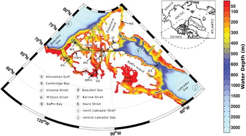
The Canadian Arctic Archipelago (CAA) is a large and complex Arctic Ocean shelf in the north of Canada (Fig. 1). It is an important connection between the Arctic and Atlantic oceans. On one hand, the CAA throughflow is a significant contributor to the net Arctic Ocean freshwater outflow (e.g., Aksenov, Bacon, Coward, & Holliday, 2010; Jahn et al., 2012; McGeehan & Maslowski, 2012; Melling et al., 2008; Prinsenberg & Hamilton, 2005), delivering cold fresh polar water (liquid freshwater) and a small amount of sea ice (solid freshwater) to the downstream Labrador Sea (Peterson, Hamilton, Prinsenberg, & Pettipas, 2012), which is an important site for open ocean deep convection (e.g., Marshall & Schott, 1999). Numerical experiments have shown that such an outflow of freshwater could significantly affect the formation of dense water and the overturning circulation (e.g., Goosse, Fichefet, & Campin, 1997; Komuro & Hasumi, 2005). On the other hand, with so many narrow straits, it also works as a buffer zone for sea ice, preventing faster outflow of multi-year sea ice from the Arctic Ocean to Baffin Bay (Sou & Flato, 2009). About 10% of the total northern hemisphere sea ice is stored within the CAA (Lietaer, Fichefet, & Legat, 2008). Because of the harsh climate and complicated network of narrow channels, the in situ or remotely sensed data available for this region has many limitations. Still, ice retreat has already been noticed in the CAA region in recent years (Howell, Duguay, & Markus, 2009).

Fig. 1 Map of the Canadian Arctic Archipelago (CAA) region. The dashed line in the inset box shows the location of the CAA (solid black curve: Northwest Passage; AG: Amundsen Gulf; QMG: Queen Maud Gulf; VS: Victoria Strait; MS: M'Clure Strait; PWS: Prince of Wales Strait; VMS: Viscount Melville Sound; MC: M'Clintock Channel; PS: Peel Sound; BS: Barrow Strait; LS: Lancaster Sound; DS: Davis Strait; QEI: Queen Elizabeth Islands; JS: Jones Sound; NS: Nares Strait). Parry Channel is the waterway running through the central CAA (MS, VMS, BS, and LS). Grey polygon represents central Parry Channel.

Besides the local oceanic and long-term climate impacts, the decline of sea ice within the CAA is also meaningful for local ecosystems. A thinner ice cover in this region possibly extends the habitat of some large marine mammals (Moore & Huntington, 2008; Wang, Myers, Hu, & Bush, 2012). Also as a consequence of ice melt, the physical properties of the ocean (e.g., sea surface temperature (SST) and sea surface salinity (SSS)) could change significantly. Although marine species do have certain abilities to adapt to a changing environment, whether they can cope with such a fast pace of climate change in the future is still in question.

In addition, the disappearance of sea ice is of importance to commercial shipping. Starting with Lancaster Sound in the east, the Northwest Passage (NWP) has three possible paths in the west (M'Clure Strait, Prince of Wales Strait, or Peel Sound, Fig. 1). The NWP provides a route between Europe and Asia that is shorter by 9000 km than the current route through the Panama Canal (e.g., Howell, Tivy, Yackel, & McCourt, 2008). Based on historical observations, Howell et al. (2008) found that a considerable amount of multi-year ice still forms in western Parry Channel and M'Clintock Channel which means that the entire NWP will still not be fully accessible in the near future, even for the least difficult route (through Peel Sound). But the sea-ice extent minima in recent years (Stroeve et al., 2008) have led to expectations that the NWP will soon become a viable shipping route.

Currently, to study ice conditions within the CAA, particularly future climate scenarios, numerical model simulations are still a necessary and effective approach. Because of the complex topography, high resolution models are needed. However, the CAA was not well resolved by most climate models in the Fourth Assessment Report by the Intergovernmental Panel on Climate Change (IPCC; Solomon et al., 2007). Thus Sou and Flato (2009) utilized a regional ice–ocean model with a resolution of 22 km to simulate sea ice within the CAA from 2041 to 2060 and found that summer concentration and thickness decreased by 45% and 36%, respectively, compared with their hindcasting run from 1950 to 2004. But there is still a lack of knowledge about the evolution of sea ice in different time periods during the twenty-first century.

The aim of this study is to simulate the possible variability of sea ice and ocean surface fields in the CAA in the context of a warmer climate with a relatively high resolution ocean–sea-ice model. First we begin with a simple description of the numerical model and data used in this study. Then the model configuration, validation, and ice conditions (concentration and thickness) for different time periods (1986–2005, 2006–2025, 2026–2045, 2046–2065, and 2066–2085) will be presented. After that, the changes in surface ocean fields (SST and SSS) will also be examined for a better perspective on the changes in sea ice. Ten sites are also selected for study of the trends in sea ice and ocean surface fields. We also examine the evolution of sea surface height (SSH) fields and their impact on fluxes through the central archipelago. A summary and discussion is provided at the end.

2 Method and data

A pan-Arctic configuration numerical model based on the Nucleus for European Modelling of the Ocean (NEMO) numerical framework version 3.1 (Madec & the NEMO team, 2008) is used in this study. This coupled ocean and sea-ice model includes a three-dimensional, free surface, hydrostatic, primitive-equation ocean component and a dynamic–thermodynamic sea-ice component. The sea-ice module is from the Louvain-la-Neuve sea-ice model (LIM2) (Fichefet & Maqueda, 1997) with a modified elastic-viscous-plastic (EVP) ice rheology (Hunke & Dukowicz, 1997). No-slip and free-slip boundary conditions are applied for sea ice and the ocean, respectively. Our model does not include a representation of fast ice, which may negatively affect our results in coastal regions.

Our model domain covers the northern Bering Sea, the Arctic seas, and part of the North Atlantic Ocean (to 45°N, see the inset in Fig. 1) with a variable horizontal resolution, from approximately 11 km within the central CAA region to approximately 15 km in the Arctic Ocean. When generating the horizontal mesh grids, an orthogonal transformation method (Murray, 1996) is used to overcome the coordinate singularity at the North Pole in standard spherical grids and provide a sufficiently high resolution in the CAA region with limited grid points. In the vertical, 46 z-levels are used with layer thickness smoothly varying from approximately 6 m at the surface to approximately 240 m at the bottom. The bathymetry data are derived from the 1 arc-minute global relief model (ETOPO1; Amante & Eakins, 2009) provided by the US National Geophysical Data Center (NGDC).

We first spin up the model for 18 years with initial ocean temperature and salinity from Polar Science Center Hydrographic Climatology (PHC 3.0; Steele, Morley, & Ermold, 2001), normal year atmospheric forcing (10 m surface wind, 10 m air temperature and specific humidity, downward longwave and shortwave radiation, total precipitation and snowfall) from the Coordinated Ocean-ice Reference Experiments-phase II (CORE-II) (Large & Yeager, 2009), monthly runoff data from a global model (ORCA05 MGP), and eastern and western open boundary data (normal and meridional velocity, temperature, and salinity) from a global simulation (ORCA025-KAB001) (Barnier et al., 2006). No temperature or salinity restoring is active except for the buffer zones close to the open boundaries and in Foxe Basin. More details can be found in Hu and Myers (2013). Starting from the spin-up state, we performed two subsequent simulations: (a) an interannual (1970–1999) simulation forced by the monthly atmospheric output (including runoff) from the twentieth century climate experiment (20C3M) of the UK Met Office Hadley Centre Coupled Model, Version 3 (HadCM3) (Gordon et al., 2000) with a horizontal resolution of 3.75° × 2.5° and (b) a “future scenario” (2000–2100) simulation forced by the monthly atmospheric output (including runoff) from HadCM3 run under the Special Report on Emissions Scenarios (SRES) A1B scenario (IPCC, 2000). Monthly ocean open boundary conditions were taken from corresponding runs of the Canadian Centre for Climate Modelling and Analysis (CCCma) Third Generation Coupled Global Climate Model CGCM3.1 (approximately 1.4° × 0.94°) (Flato & Boer, 2001). Synoptic-scale weather variability may also affect sea-ice conditions within the CAA, For example, ice deformation could be much higher with more variable wind forcing, which is underestimated in the monthly mean wind data (particularly the magnitude near the coastlines); however, inclusion of these considerations is beyond the scope of this study.

Because of the low resolution of atmospheric model fields, we were concerned that local biases could affect the high resolution ocean simulations. Applying the changes in original fields onto relatively higher resolution climatological fields might help avoid part of the bias. Here, we employ a similar approach to Dumas, Flato, and Brown (2006), adding the difference between the monthly output from HadCM3 and the average over 1970–1999 to the climatology (CORE-II normal year data). For “large” value variables (surface air temperature and downward radiation), we added the mathematical difference from the mean to climatology

where X _new is the new value; X _ori is the output from HadCM3; is the CORE-II normal year value; is the average of the output from HadCM3 for 1970 to 1999, and t is time. For “small” value variables (precipitation, snowfall, and specific humidity), we multiplied the climatology by a ratio (to avoid negative values) between the original output and the mean

We applied the runoff and vector fields (u- and v-wind) without any modification. With this pre-processing, on one hand the re-created forcing includes variations in the corresponding HadCM3 field, which allows us to study the responses of the sea ice and ocean to the changes in the HadCM3 forcing. On the other hand, it guarantees a reasonable seasonal cycle by taking advantage of the CORE climatology data as the base.

Another parallel interannual simulation using CORE-II interannual reanalysis forcing data was conducted to validate the model configuration by comparing the output with the observations. Observed ice concentration from the Canadian Ice Service Digital Archive (CISDA) is used to evaluate the simulated seasonal and interannual variabilities. Simulated sea ice in the CAA from two Coupled Model Intercomparison Project, Phase 5 (CMIP5) experiments, the Geophysical Fluid Dynamics Laboratory–Earth System Models GFDL-ESM2M and GFDL-ESM2G (Dunne et al., 2012), run under the Representative Concentration Pathways 6.0 (RCP6.0) scenario, is also used to examine trends in the twenty-first century. The equivalent CO₂ concentration in scenario RCP6.0 reaches a level close to that in scenario A1B by the end of the twenty-first century. Of the two CMIP5 models, GFDL-ESM2G has a better horizontal resolution in the CAA region.

3 Results

In this section, we first demonstrate how well the model can reproduce the response of the ice fields to the atmospheric forcing. The differences in ice concentration and thickness between the simulations using CORE-II and HadCM3 forcing are also presented. Second, we will focus on the sea-ice condition variations in future time slices (2006–2025, 2026–2045, 2046–2065, and 2066–2085) over Canadian Arctic waters and at select sites. Third, we will present the changes in ice and ocean fluxes through the central CAA. The changes in ocean surface properties (temperature and salinity) will also be presented at the end.

a Model Configuration Validation

Due to the biases in forcing data, it is not proper to validate the model configuration by directly comparing the observations and model output using HadCM3 forcing even with the “patch” mentioned in Section 2. It is also known that there are issues in producing observation-like ice fields (concentration, thickness, and circulation) in global climate models (Kwok, 2011). Thus, the outputs from a parallel interannual simulation using CORE-II forcing are used first in this section.

Generally, reasonable ice fields are simulated by the model in the CAA region. The simulated seasonal cycle (averaged for 1986 to 1999) of ice concentration agrees with CISDA data, with an ice concentration close to 1 during the cold season (December, January–April) and a minimum ice concentration of approximately 0.4 ± 0.07 in September (Fig. 2a), although the model concentrations are lower in the warm season (July–October) by approximately 0.16, on average. The largest differences occur in July (0.24) and October (0.17), indicating fast melting and slow freeze-up, respectively, These values are outside the lower bound of the observation standard deviations (STDs) (0.05 and 0.10, respectively). Ice thickness responds to atmospheric forcing with a time lag of one to two months, resulting in a seasonal cycle with a maximum of approximately 2.28 ± 0.23 m in May and a minimum of approximately 1.27 ± 0.31 m in and October (Fig. 2b). The STDs are relatively large in the warm season (July: 0.28, August: 0.35, September: 0.39, and October: 0.31), suggesting higher interannual variabilities during those months.

Fig. 2 (a) Seasonal cycle of ice concentration and (b) thickness within the CAA (Nares Strait, Baffin Bay, and Foxe Basin excluded) averaged over 1986–1999 (grey solid line: Canadian Ice Service Digital Archive data; black solid line: model simulation using CORE-II forcing; black dashed line: model simulation using HadCM3 forcing; bars: standard deviation).

During the cold season, ice covers all of the northern CAA, the CAA channels (including Nares Strait), and Baffin Bay almost completely southward to Davis Strait except near the west coast of Greenland (Fig. 3a). The spatial pattern is in agreement with observations (CIS, 2002), although the land-fast ice (e.g., along northeastern Baffin Bay) is not captured. Thicker sea ice of 3–4 m is located along the northern coast of the CAA and Greenland, which is consistent with previous studies (e.g., Bourke & Garrett, 1987), although thinner. Within the Queen Elizabeth Islands (QEI), simulated ice thickness is close to the late winter average value, 3.4 m, estimated by Melling (2002) in the 1970s using drill hole measurements. The decline in ice thickness from the northwestern to southeastern Sverdrup Basin (QEI, west of 100°W) noticed by Melling (2002) is also reproduced by the model, indicating a reasonable transition of sea ice from the Arctic coast to the central CAA. Within Parry Channel, a positive eastward gradient is found in ice thickness, with thicker ice on the Arctic Ocean side and thinner ice on the Baffin Bay side with some thick ice adjacent to M'Clintock Channel (Fig. 3e). Within Baffin Bay, ice is generally thicker on the west side.

Fig. 3 Simulated 1986–1999 cold season (December, January–April) and warm season (July–October) (a–d) ice concentration and (e–h) thickness using CORE-II forcing (a, c, e, and g) and HadCM3 forcing (b, d, f, and h).

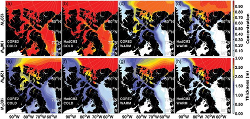
During the warm season, a north–south pattern separated by Parry Channel is clearly shown both in concentration and thickness, with high concentration and thick sea ice in the north (including the QEI) and low concentration and thin sea ice in the south (Figs 3c and 3g), with M'Clintock Channel being an exception. Ice thickness within the QEI becomes thicker along the path towards the central CAA, which is a result of the influx of multi-year sea ice from the north. In the central CAA, sea ice with a high concentration is found in the western half of Parry Channel, especially to the south, and M'Clintock Channel (Fig. 3c), which is in agreement with observations (CIS, 2002). Such an along-channel spatial pattern is not obvious in the thickness field (Fig. 3g). Sea ice in Jones Sound does not melt as much as observed (CIS, 2002). The eastern half of Baffin Bay is nearly ice free while some ice with a concentration <0.5 and thickness <1 m is confined to the west coast (Figs 3c and 3g).

Because the CAA is covered by sea ice during most of each year, the interannual variation in the ice fields during the warm season is most interesting. With CORE-II forcing, the interannual variation in the warm season ice concentration within the CAA is also reasonably reproduced compared with CISDA data (Fig. 4). Again, simulated concentrations are generally lower, which is caused by faster melting in the model from May to July (Fig. 2a), which was also noticed by Sou and Flato (2009). Overall, the model successfully captures the high (e.g., in 1986 and 2004) and low (e.g., in 1998 and 2007) ice events in the past (Fig. 4) with a correlation coefficient of 0.68.

Fig. 4 Interannual variability of the CAA (as in Fig. 2) warm season ice concentration over 1980–2007 (grey solid line: CISDA data; black solid line: model simulation using CORE-II forcing; black dashed line: model simulation using HadCM3 forcing).

Compared with the simulation using CORE-II forcing, the simulation with HadCM3 forcing produces a similar seasonal cycle of ice concentration (Fig. 2a) and thickness (Fig. 2b) but with much lower ice concentration in summer and approximately 0.2 m thinner, on average, throughout the year. Generally, the simulated concentration and thickness fall into the range of interannual variations of that using CORE-II forcing (except for the concentration in November). However, the STDs for thickness are much smaller compared to those for CORE-II forcing. It indicates weaker interannual variabilities in the HadCM3 forcing from 1986 to 1999. With HadCM3 forcing, both concentration and thickness reach the minimum at almost the same time, August to September, without the time lag noticed with CORE-II forcing.

The large-scale spatial pattern of the sea-ice fields in this simulation are similar to those using CORE-II forcing (Fig. 3). But the thick ice in HadCM3 covers a much larger area to the north of the CAA, extending into the central Arctic Ocean, all year round (Figs 3f and 3 h). The ice is much thinner in the southern parts, with an almost ice-free Baffin Bay in the warm season (Figs 3d and 3 h). There is no regional thick or high concentration sea ice found in M'Clintock Channel (Figs 3d and 3f). Therefore, the results in the following sections need to be considered with caution because an earlier ice-free CAA could be simulated when using HadCM3 forcing fields.

b Sea Ice Conditions in Future Periods

1 Trends for sea ice in the Canadian Arctic Archipelago

As expected, in the context of a warmer climate, ice in the CAA declines in all seasons (winter: January–March; spring: April–June; summer: July–September; and autumn: October–December) both in concentration (Fig. 5a) and thickness (Fig. 5b). Ice concentration decreases least in winter, with only negligible reductions close to the end of our simulation. In summer and autumn, a rapid decrease is found from the beginning of the 2030s to the end of the 2040s. From 2026 to 2065, ice concentration decreases by approximately 0.29 in summer (65%) and autumn (38%). With this simulation, it shows that even in summer, the CAA could be completely ice free only by the end of the twenty-first century. In the CMIP5 models, ice concentration is relatively stable until the beginning of the 2040s (Figs 5c and 5e). From the 2040s, a similar decrease in summer concentration is shown in GFDL-ESM2G but without significant change in autumn. After a sharp increase at the end of 2040s, the GFDL-ESM2M also produces an accelerated decrease in summer and autumn concentrations.

Fig. 5 Simulated interannual variation of the averaged seasonal ice concentration (a, c, and e) and thickness (b, d, and f) within the CAA (as in Fig. 2) over the 1980–2099 period in our simulation with HadCM3 forcing (top row), GFDL-ESM2G (RCP6.0, centre row), and GFDL-ESM2M (RCP6.0, bottom row) (solid black line: January–March; grey solid line: April–June; black line with plus sign: July–September; grey line with plus sign: October–December; dotted lines in (a): data from the CISDA).

Compared with ice concentration, thinning of ice is notable during all four seasons in our entire simulation (Fig. 5b). The decreases are limited before 2006 but accelerate after that. From 2026 to 2065, on average, there is a reduction of approximately 0.22 m per decade in the annual mean from 1.68 m. The net reductions are similar in all four seasons but the proportional reductions differ based on the initial values (e.g., in summer, 0.25 m per decade from 1.33 m leads to a thinning of approximately 75% but only 49% in spring from 2.05 m. By the end of this simulation, the seasonal sea ice still reaches a thickness of approximately 1 m in winter and spring. Regardless of the initial values and the time shift, GFDL-ESM2G produces a similar trend in the CAA ice thickness: a faster decrease following a slow decrease period. The shift happens around 2050. In GFDL-ESM2M, the trend in thickness is similar to that in concentration, showing a decreasing trend after a recovery at the end of the 2040s.

Compared with our simulation, both of the CMIP5 models show larger fluctuations in time as well as seasonal cycle (particularly in thickness before the CAA reaches an ice free summer); this may be because they are coupled models that have better two-way feedbacks between the atmosphere and ocean (e.g., Dorn et al., 2007; Döscher et al., 2002). This is also shown in the following ice thickness field. Compared with GFDL-ESM2G, GFDL-ESM2M produces much thinner and lower sea-ice concentration in the CAA, which leads to almost zero summer thickness even in the 2020s. Apart from the differences in model settings, the model horizontal resolution in the CAA must also play a role. In GFDL-ESM2M, only the major passages exist, which are poorly resolved and artificially widened; this might make the ice more dynamic without ice blocking narrow passages, thus producing thinner sea ice in the CAA. However, free-ice drift is not the case all the time in the CAA with ice observed to block narrow channels (Agnew, Lambe, & Long, 2008).

2 Changes in sea ice spatial pattern

In winter, changes in visible ice concentration are only found in Amundsen Gulf and Baffin Bay (Figs 6a to 6d). Ice thickness decreases more significantly in the Arctic Ocean where multi-year ice is located, especially during 2046–2065 and 2066–2085 (Figs 6i to 6l). Reduction in ice thickness in the central CAA and Baffin Baffin is very small during 2006–2025 and 2026–2045. At the same time ice thickness increased by approximately 0.5 m regionally within the QEI (Figs 6i and 6j), which may be caused by the motion of multi-year sea ice inflowing from the north. This gain is lost later during 2046–2065 (Fig. 6k). Most ice within Parry Channel and M'Clintock Channel starts thinning in the 2046–2066 period.

Fig. 6 (a) to (d) and (i) to (l) Winter (January–March) and (e) to (h) and (m) to (p) summer (July–September) (a) to (b) ice concentration and (i) to (p) thickness in four time periods (1st column: 2006–2025; 2nd column: 2026–2045; 3rd column: 2046–2065; 4th column: 2066–2085).

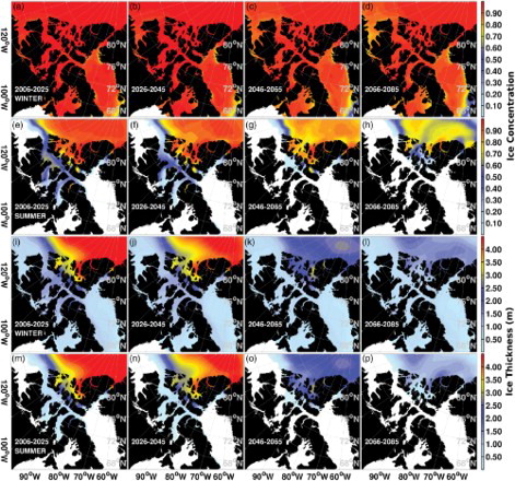
In summer, the changes are more dramatic compared with winter (Figs 6e to 6h and 6m to 6p). The west part of the NWP, from Amundsen Gulf to Queen Maud Gulf, is open during all four time periods. That the route through Peel Sound will be the earliest accessible route, as Howell et al. (2008) mentioned, is also supported by our simulation. The east part of the NWP, from Victoria Strait to Peel Sound and Lancaster Sound, is partly open (but not for the entire summer) during 2046–2065 and 2066–2085. In the 2006–2025 and 2026–2045 periods, Parry Channel is still covered by sea ice with a concentration of approximately 0.5, especially in the Viscount Melville Sound region prior to 2026. Compared with the sea ice in 1986–2005, ice in the central region, close to Barrow Strait, actually increases in thickness by approximately 1.0 m (see Section 3b3 for details), which delays the opening of all of Parry Channel in 2046–2066 (Fig. 6f and 6n). Pronounced retreat and thinning of sea ice is found in the northern part of the CAA (QEI and northern coast) and interior of the Arctic Ocean in 2046–2065 and 2066–2085. The thick multi-year ice pack, located to the north of the CAA, has a thickness of approximately 2 m and a concentration of approximately 0.8 m in 2046–2065, and approximately 1.5 m and approximately 0.7, respectively, in 2066–2085. Because Baffin Bay is ice free during summer, no change is observed in those figures.

3 Changes in sea ice at select sites

In this section, ten sites (see Fig. 1) are selected to represent the NWP (Amundsen Gulf, Cambridge Bay, Victoria Strait, M'Clure Strait, Barrow Strait) and its upstream (Beaufort Sea) and downstream ends (Baffin Bay, Davis Strait, northern Labrador Shelf, and central Labrador Sea). The location of each site is given in Table 1. The annual mean ice concentration and thickness with STDs for each period at each site are summarized in Tables 2 and 3, and their interannual variations in different seasons are presented in Figs 7 and 8.

Fig. 7 Simulated interannual variation of the averaged seasonal ice concentration at the selected sites (locations are given in Fig. 1 and Table 1) for the 1980–2099 period (solid black line: January–March; grey solid line: April–June; black line with plus sign: July–September; grey line with plus sign: October–December).

Fig. 8 As in Fig. 7 but for ice thickness.

Table 1. Locations of select sites (average taken over a neighbouring region of 5 × 5 model grid cells).

Site	Longitude	Latitude
Amundsen Gulf	122.30°W	70.40°N
Cambridge Bay	106°W	69°N
Victoria Strait	99°W	70.5°N
Beaufort Sea	136°W	78°N
M'Clure Strait	123°W	75.2°N
Barrow Strait	95°W	74.35°N
Baffin Bay	65°W	72°N
Davis Strait	58°W	67°N
North Labrador Shelf	62°W	59°N
Central Labrador Sea	51°W	57°N

Table 2. Annual mean ice concentration with standard deviation at the select sites (see Fig. 1 and Table 1 for the locations) during different time periods.

Site	1986–2005	2006–2025	2026–2045	2046–2065	2066–2085
Amundsen Gulf	0.63 ± 0.08	0.54 ± 0.04	0.48 ± 0.04	0.44 ± 0.04	0.38 ± 0.03
Cambridge Bay	0.55 ± 0.03	0.52 ± 0.02	0.50 ± 0.03	0.45 ± 0.03	0.44 ± 0.02
Victoria Strait	0.76 ± 0.05	0.74 ± 0.04	0.67 ± 0.04	0.53 ± 0.04	0.52 ± 0.02
Beaufort Sea	0.97 ± 0.01	0.96 ± 0.01	0.95 ± 0.01	0.92 ± 0.01	0.86 ± 0.10
M'Clure Strait	0.86 ± 0.06	0.76 ± 0.07	0.63 ± 0.08	0.50 ± 0.05	0.49 ± 0.06
Barrow Strait	0.55 ± 0.04	0.75 ± 0.10	0.78 ± 0.05	0.61 ± 0.06	0.56 ± 0.02
Baffin Bay	0.56 ± 0.04	0.56 ± 0.03	0.53 ± 0.04	0.48 ± 0.02	0.48 ± 0.02
Davis Strait	0.38 ± 0.09	0.41 ± 0.04	0.37 ± 0.06	0.32 ± 0.04	0.29 ± 0.05
North Labrador Shelf	0.36 ± 0.05	0.35 ± 0.04	0.31 ± 0.05	0.23 ± 0.04	0.19 ± 0.06
Central Labrador Sea	0.00 ± 0.00	0.00 ± 0.00	0.00 ± 0.00	0.00 ± 0.00	0.00 ± 0.00

Table 3. As in Table 2 but for ice thickness (unit: m).

Site	1986–2005	2006–2025	2026–2045	2046–2065	2066–2085
Amundsen Gulf	0.73 ± 0.17	0.54 ± 0.06	0.44 ± 0.04	0.39 ± 0.03	0.33 ± 0.03
Cambridge Bay	0.59 ± 0.06	0.55 ± 0.05	0.52 ± 0.05	0.43 ± 0.06	0.43 ± 0.03
Victoria Strait	1.03 ± 0.10	0.99 ± 0.10	0.82 ± 0.09	0.52 ± 0.07	0.51 ± 0.03
Beaufort Sea	4.09 ± 0.18	3.84 ± 0.23	3.28 ± 0.65	2.11 ± 0.22	1.79 ± 0.48
M'Clure Strait	1.49 ± 0.18	1.22 ± 0.20	0.92 ± 0.13	0.56 ± 0.10	0.63 ± 0.13
Barrow Strait	0.91 ± 0.11	1.20 ± 0.18	1.16 ± 0.17	0.69 ± 0.15	0.57 ± 0.03
Baffin Bay	0.52 ± 0.11	0.52 ± 0.06	0.50 ± 0.08	0.38 ± 0.04	0.40 ± 0.03
Davis Strait	0.41 ± 0.17	0.40 ± 0.07	0.35 ± 0.10	0.25 ± 0.04	0.23 ± 0.07
North Labrador Shelf	0.38 ± 0.06	0.35 ± 0.05	0.30 ± 0.06	0.19 ± 0.04	0.17 ± 0.05
Central Labrador Sea	0.00 ± 0.00	0.00 ± 0.00	0.00 ± 0.00	0.00 ± 0.00	0.00 ± 0.00

The Beaufort Sea is the region where the Arctic Ocean experiences great changes in sea ice. While the annual mean ice concentration is relatively stable, with a value >0.95 (Table 2), ice thickness shows a decreasing trend (Table 3) with large interannual variations before the 2030s. Ice concentration in summer and autumn drops abruptly at the end of 2070s (Fig. 7d) (e.g., in summer, from >0.8 to approximately 0.2 within 10 years). Ice thickness evolves similarly in all four seasons (Fig. 8d), and significant thinning is found after the 2030s, which is much earlier than the reduction in concentration. By the 2050s, a thickness of approximately 2 m, which is only half the value at the beginning of the twenty-first century, is simulated.

In Amundsen Gulf and Cambridge Bay, there is only seasonal ice during the model integration (Fig. 7a), with an annual mean concentration of approximately 0.5 and thickness of approximately 0.5 m since the beginning of this century (Tables 2 and 3). The NWP though Peel Sound is blocked by relatively thicker sea ice in Victoria Strait, with a mean concentration >0.5 and thickness >0.8 m before 2050 (Tables 2 and 3). In summer, the NWP may be ice free from 2050 but this is not likely to happen in other seasons (Fig. 7).

M'Clure Strait, the gate of another NWP route, is covered by sea ice with an even higher concentration (>0.06) and thickness (>0.9 m) compared with the sea ice in Victoria Strait before 2050. With a value >0.8 in all four seasons at the beginning of the integration, the ice concentration decreases much faster in summer, reaching as low as 0.1 around 2020 while there are decreases of only 25% and 50% in spring and fall, respectively, by 2050. However, summer ice concentration rebounds (although it is still <0.5) with large interannual variability over the next 20 years, and then is almost icefree for the remainder of the model integration. Summer and autumn ice thickness decrease by approximately 50% by the beginning of the 2020s. It then takes about another 30 years for the winter and spring ice to decay.

In Barrow Strait, the change in sea ice is quite different (Figs 7f and 8f). Instead of a decreasing trend, there is an abrupt increase in both ice concentration and thickness from 2008 to 2046. However, there is no cooling signal in the atmospheric forcing, which indicates that these changes are caused by accumulation resulting from ice advection (see details in Section 3c1).

Downstream of the CAA, seasonal ice forms in Baffin Bay, Davis Strait, and on the Labrador Shelf (Figs 7g to 7i and 8g to 8i). There is no ice in the central Labrador Sea all year (Figs 7j and 8j). In central Baffin Bay, both the concentration and thickness show little variation in their annual means. A decrease of approximately 0.1 in spring and autumn concentration and 0.2–0.3 m in autumn, winter, and spring thickness occur around the end of the 2040s. In Davis Strait, even in the autumn, the concentration (<0.2) of thin (<0.2 m) ice is very low before 2046. The northern Labrador Shelf is similar, being almost ice free both in the autumn and summer, particularly after the 2040s. A reduction of approximately 50% in winter and spring concentration and thickness occurs in the 2040s. Large interannual variations are found in winter and spring sea ice in Davis Strait and on the northern Labrador Shelf.

c Changes in Ice and Ocean Fluxes Through the Central Canadian Arctic Archipelago

1 Impact of sea surface height on the central Parry Channel ice flux

Central Parry Channel (grey polygon in Fig. 1) is one of the regions with multi-year ice (both locally formed as well as advected from the QEI and western Parry Channel) in the CAA (e.g., Howell et al., 2008). Thus, it plays an important role in the opening of the NWP, particularly the routes through M'Clure Strait or Prince of Wales Strait.

In our simulation (using HadCM3 forcing), more sea ice is simulated in central Parry Channel (Figs 9a and 9b) during the 2006–2045 period, particularly in summer (with a concentration of approximately 0.5 and thickness of approximately 1 m). We analyzed the atmospheric fields (surface air temperature and net downward shortwave and longwave radiation) and found that the increase in sea ice is not likely caused by heat fluxes from the atmosphere into the ocean (not shown here). This is also supported by the ice production (positive values mean an increase in ice) in this region (Fig. 9c). Ice growth actually decreases slightly in fall and winter, while significant melt in July to September occurs in the model. Thus, the extra ice is related to a reduction in ice melt and export during the April–June period. So how is this related to the ice dynamics during this time period?

Fig. 9 Simulated interannual variation of the averaged seasonal (a) ice concentration, (b) thickness, and (c) ice production within central Parry Channel (grey polygon in Fig. 1). Solid black line: January–March; solid grey line: April–June; black line with plus sign: July–September; grey line with plus sign: October–December.

The ice fluxes (April–June) from the four sides of Parry Channel are presented in Fig. 10a. A positive value means an accumulation in this region. It shows that the net ice flux is dominated by the eastward export through Barrow Strait, which reduces significantly to almost zero before the time period of interest. Therefore, the reduction in ice export through Barrow Strait results in an accumulation of ice in the April–June period, and later thicker ice with a higher concentration in the July–September period. Because there is insufficient heat available from the atmosphere (as well as the underlying ocean) to melt this additional ice, the accumulated ice remains in central Parry Channel year round.

Fig. 10 (a) Ice fluxes from four directions (north, west, south, and east) into and out of central Parry Channel (grey polygon in Fig. 1, positive: into the region) and (b) major cross-channel component momentum terms (thick solid black line: Coriolis term; dotted black line: sea surface height gradient term; thin solid grey line: wind stress term; dashed black line: initial sea surface height gradient term in 1980 plus the salinity-induced changes in this term) at Barrow Strait averaged for April–June.

To determine the dynamic factor(s) affecting ice flux through Barrow Strait, the ice momentum balance is provided here. For the cross-channel component, the momentum equation is given by:

where x and y represent the along- and cross-channel directions, respectively; u is along-channel ice velocity; v is cross-channel ice velocity; f is the Coriolis parameter; g is the acceleration due to gravity; η is the sea surface height; τ_a is the wind stress; τ_w is the ocean stress; ρ_i is the density of ice; H is ice thickness; and σ_y is the y-component of internal ice stress.

Figure 10b shows the three major terms, the Coriolis term (fu), the SSH gradient term , and the wind stress term . The residuals are balanced by the remainder of the terms. This shows that the ice motion is mainly geostrophic, with the SSH gradient term balancing the Coriolis term. The decrease in the cross-channel SSH gradient leads to a slowdown in the along-channel ice velocity and thus the ice flux. The local wind stress actually contributes very little to the cross-channel ice momentum balance, at least prior to the late 2030s. The role of local wind stress becomes more important as the ice concentration and thickness decrease.

Based on the analysis of salinity- and temperature-induced SSH gradient terms, we found that the changes in the cross-channel SSH gradient above to be dominated by the cross-channel salinity change (Fig. 10a). The detailed calculation of salinity- and temperature-induced SSH is presented in Hu and Myers (2013). Salinity and temperature changes in the top 250 m of the water column are considered in our calculation with reference fields from April to June 1980.

2 Impact of sea surface height on the central Canadian Arctic Archipelago volume and freshwater fluxes

Within a wide enough channel, the cross-channel SSH gradient is initially set by the geostrophic adjustment of the channel throughflow. Thus, as the cross-channel SSH gradient changes, we expect such changes to be linked with the evolution of the large-scale SSH differences both upstream and downstream of Parry Channel, which impacts the throughflow. We find that the large differences are associated with the uplift of SSH in Baffin Bay.

Figure 11a shows the monthly simulated volume transport through western Lancaster Sound against the 1999–2010 mooring data (Peterson et al., 2012). A zoom of the overlapping time period is shown in Fig. 11b. The model estimates the volume transport to be 0.66 Sv (1 Sv = 10⁶ m³ s⁻¹) for 1999–2000, which is slightly higher than observed (0.49 Sv). The model captures the general features of the seasonal cycle, with a maximum in the summer months (July–September) and lows in the winter months, although the seasonal amplitude range is smaller than observed. In terms of interannual variations, the enhanced flow during the 2000–2001 period is partly reproduced; however, the transport reduction observed during the 2007–2008 period is not found in the simulation. The overall correlation coefficient between the monthly time series is 0.41 (significant at the 95% level).

Fig. 11 (a) to (d) Simulated (blue solid line) versus observed (red solid line) Lancaster Sound (a) and (b) volume flux and (c) and (d) freshwater flux over (a) and (c) the model simulation and (b) and (d) zoomed into 1999–2010. (e) Annual mean SSH along the track (Fig. 11g) over the model simulation; (f) shows the SSH difference (black line, – , right-axis, unit: m) versus Lancaster Sound volume transport (blue line, left-axis, unit: Sv). (g) Map of the central CAA (grey shading indicates water depth; the solid line indicates the track for SSH calculation). The zero lines in (a) to (d) are shown as dashed horizontal lines.

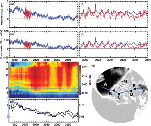
In our simulation, the freshwater flux through Lancaster Sound (Fig. 11c) is dominated by volume transport (correlation coefficient >0.95). The average freshwater flux over the 1999–2000 period is 53 mSv (1 mSv = 10³ m³ s⁻¹), which is higher than observed (34 mSv). This is mainly a result of the higher volume flux in the model. The correlation coefficient between the monthly simulated and observed freshwater fluxes over the 1999–2010 period is 0.48 (significant at the 95% level, Fig. 11d).

Over the simulation, the central CAA throughflow is strong in the 1980s and early 1990s and generally decreases during the twenty-first century with IPCC A1B climate scenario forcing (Fig. 11a). It decreases more significantly after 2020, even with westward flow toward the Arctic Ocean in some years after 2040.

To explain these changes, SSHs are extracted along a track (Fig. 11g) from the interior of the Canadian Basin, along the centre line of Parry Channel, to the interior of Baffin Bay and shown as a Hovmöller diagram in Fig. 11e. An SSH gradient exists along the track, with generally higher SSHs on the west side (Arctic Ocean) and lower SSHs on the east side (Baffin Bay). The annual SSH differences (black solid line in Fig. 11f) between the west (averaged between points B and C in Fig. 11g) and the east ends (averaged between points D and E in Fig. 11g) are found to be highly correlated to the central CAA throughflow volume transport (blue solid line in Fig. 11f), with a correlation coefficient of 0.86 (significant at the 95% level). Most of the variance is caused by changes in SSH close to the mouth of Lancaster Sound in Baffin Bay. This is consistent with McGeehan and Maslowski (2012), who found a similar correlation coefficient between the SSH difference and the central CAA volume transport. But McGeehan and Maslowski (2012) used a different location (point M in Fig. 11g) to represent the Arctic Ocean SSH. Why do we get the same results with a different upstream point? We think there are two possible reasons. One is that the variations are mainly determined by changes in downstream SSHs. The other is that waters passing through M'Clure Strait and point M (Fig. 11g) have similar sources of variability (e.g., Houssais & Herbaut, 2011).

d Ocean Surface Conditions in Future Periods

1 Trends in Sea Surface Temperature and Sea Surface Salinity within the Canadian Arctic Archipelago

Within the CAA, SST shows a pronounced increase in summer and autumn in the 2040s and onward (Fig. 12a). During the 2040s, the surface ocean warms from approximately 0° to approximately 2°C, which corresponds to both an increase in surface air temperature and a decrease in ice cover at the same time. At the same time, although not as noticeable, SST increases by 0.6°C in autumn. As most areas of the CAA are covered by sea ice in winter and spring, there is only a slight increase (less than 0.4°C in total) in SST, which is otherwise close to the freezing point of sea water, in the latter half of the integration.

Fig. 12 (a) Simulated interannual variation of the averaged seasonal sea surface temperature, (b) salinity and ocean surface freshwater flux within the CAA (as in Fig. 2) for the 1980–2099 period (solid black line: January–March; solid grey line: April–June; black line with plus sign: July–September; grey line with plus sign: October–December).

However, no trend in the simulated SSS is indicated over the entire integration in all seasons within the CAA (Fig. 12b). The SSS field demonstrates a strong seasonal cycle with a range of 1, with the lowest salinity occurring in summer due to ice melt and the highest salinity occurring in winter and spring caused by ice formation (Fig. 12c). Note that Fig. 12c shows the total surface freshwater flux into the ocean (including precipitation, runoff, and ice–water conversion, referenced to a salinity of 34.7 in the model). A positive value means dilution of the ocean surface while a negative value means concentration. Figure 12c shows more freshwater loss in autumn than winter, which is consistent with the ice formation in Figs 5a and 5b. Also the contribution of freshwater input in spring and summer switches after approximately 2040, indicating an earlier melt season. The decrease in freshwater input in summer by the end of the twenty-first century is also due to less sea ice remaining after the enhanced spring melt. On average, there is no clear trend in the net ocean surface freshwater input during the April–September period. It is the decrease in fall and winter ice formation, especially fall, that results in a slightly weaker seasonal cycle of SSS over approximately the last 15 years. A decadal oscillation with a period of approximately 40 years exists in the SSS field, with high SSS at the beginning of the 2000s, 2050s, and 2090s. In addition to the surface processes represented by the ocean surface freshwater fluxes, changes in the lateral inputs (i.e., upstream inflow of fresher polar water and downstream intrusion of saltier water from Baffin Bay), which are related to large-scale atmospheric and oceanic circulation changes, also play a role in the SSS fluctuations.

2 Changes in Sea Surface Temperature and Sea Surface Salinity spatial patterns

In winter, local melt of sea ice (Figs 6a to 6d) leads to lower SSTs along the west Greenland coast up to the southern end of Nares Strait, especially in the region close to the eastern part of Davis Strait (Figs 13a to 13d). The central Arctic Ocean and most of the CAA waters are still close to the freezing point of seawater because of the existence of ice cover in 2005–2025 and 2026–2045. In winter, the Beaufort Sea and Amundsen Gulf experience the most significant warming in our simulation, locally as high as approximately 0.1°C in 2046–2065 and approximately 0.2°C in 2066–2068, compared with 1986–2005. At the same time, surface freshening >0.75 is first seen in Baffin Bay coastal and adjacent regions (west Greenland coast, Nares Strait, Jones Sound, and the eastern part of the QEI) in 2006–2025 (Fig. 13i). This freshening extends to the northern coast of the CAA in 2026–2045 (Fig. 13j). Later, freshening is also found in the central Arctic Ocean, particularly the Beaufort Gyre in 2066–2085 (Fig. 13l). The freshening demonstrates a north–south spatial pattern. In Baffin Bay, there is no freshening signal along the eastern coast of Baffin Island where the southward flow carries a mix of cold fresh water southward. Within the CAA, freshening occurs mainly in the waters north to Parry Channel.

Fig. 13 (a) to (d) and (i) to (l) Winter (January–March) and (e) to (h) and (m) to (p) summer (July–September) (a) to (h) sea surface temperature (SST) and (i) to (p) sea surface salinity (SSS) anomalies in four time periods (1st column: 2006–2025; 2nd column: 2026–2045; 3rd column: 2046–2065; 4th column: 2066–2085) compared with these fields for the 1986–2005 seasons. Note that the colours for SSS are used in reverse order from the SST plots.

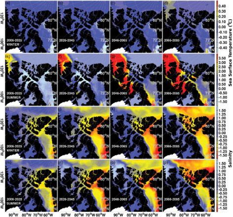
In summer, without the heat loss due to ice melt, the warming of the sea surface is much more significant (Figs 13e to 13h). The warming is first seen in the southern Beaufort Sea and Amundsen Gulf in 2006–2025, which then extends to the central Beaufort Sea reaching the mouth of M'Clure Strait in 2026–2045. The amplitude increases at the same time. Later the western parts of Parry Channel, M'Clintock Channel, and Baffin inlets (Prince Regent Inlet and Gulf of Boothia), as well as the eastern coast of Baffin Island, warm in 2045–2065 and 2066–2085. The freshening in summer has a similar north–south pattern to that in winter but is slightly larger in amplitude, particularly in the the central Arctic Ocean (Fig. 13m to 13p). Another difference is that in ice-free regions (e.g., southern Beaufort Sea, Amundsen Gulf and M'Clintock Channel) SSS increases because of relatively less ice melt in the future. This spatial variation in the trend for SSS also explains why there is no monotonic decrease in SSS over the entire CAA region. In addition, cooling in central and eastern Parry Channel in 2006–2025 and 2026–2045, corresponds to more ice melt occurring there (Section 3c1).

3 Changes in Sea Surface Temperature and Sea Surface Salinity at select sites

As mentioned in the previous section, the trends in ocean surface variables, especially SSS, vary in space. In terms of the annual mean, the ocean surface warms at all ten selected sites by 2066–2085 (Table 4), increasing by as much as 2.38°C in the central Labrador Sea and as little as 0.15°C in the Beaufort Sea. The trends for SSS at the ten sites are varied (Table 5). Without considering ocean circulation, the changes in ocean surface freshwater flux can explain the evolution of SSS at most sites. For the seasonal cycle of SSS at locations covered or seasonally covered by sea ice, the ocean surface freshwater flux is dominated by ice formation and melt processes (an annual mean precipitation of 10⁻⁵kg m⁻² s⁻¹ is equivalent to an annual melt of approximately 0.38 m with a salinity of 6 and a reference salinity of 34.7). In winter, less ice forms locally, indicating less brine ejected into the ocean and lower SSS. In summer, more ice melts locally, signalling more freshwater flux into the ocean and again lower SSS. Tables 4 and 5 present the annual mean SST and SSS at each site, and Figs 14 and 15 show their interannual variations during the different seasons.

Fig. 14 Simulated interannual variation of the averaged seasonal sea surface temperature at the select sites over the time period 1980–2099 (solid black line: January–March; solid grey line: April–June; black line with plus sign: July–September; grey line with plus signs: October–December).

Fig. 15 As in Fig. 14 but for sea surface salinity.

Table 4. As in Table 2 but for sea surface temperature (unit: °C).

Site	1986–2005	2006–2025	2026–2045	2046–2065	2066–2085
Amundsen Gulf	−0.59 ± 0.61	0.10 ± 0.41	0.68 ± 0.44	1.06 ± 0.45	1.64 ± 0.48
Cambridge Bay	0.21 ± 0.27	0.46 ± 0.36	0.53 ± 0.32	1.16 ± 0.39	1.34 ± 0.35
Victoria Strait	−1.48 ± 0.17	−1.44 ± 0.15	−1.10 ± 0.29	−0.09 ± 0.32	0.00 ± 0.25
Beaufort Sea	−1.73 ± 0.02	−1.71 ± 0.01	−1.67 ± 0.01	−1.66 ± 0.01	−1.57 ± 0.19
M'Clure Strait	−1.64 ± 0.04	−1.53 ± 0.14	−1.22 ± 0.28	−0.41 ± 0.33	−0.52 ± 0.41
Barrow Strait	−1.02 ± 0.18	−1.58 ± 0.14	−1.59 ± 0.11	−0.90 ± 0.30	−0.62 ± 0.19
Baffin Bay	−0.31 ± 0.38	−0.41 ± 0.25	−0.13 ± 0.37	0.37 ± 0.22	0.27 ± 0.16
Davis Strait	0.86 ± 0.91	1.23 ± 0.41	1.62 ± 0.64	2.18 ± 0.30	2.41 ± 0.44
North Labrador Shelf	1.14 ± 0.41	1.29 ± 0.45	1.70 ± 0.59	2.65 ± 0.47	2.81 ± 0.57
Central Labrador Sea	5.25 ± 0.58	6.13 ± 0.69	6.42 ± 0.96	7.50 ± 0.33	7.63 ± 0.42

Table 5. As in Table 2 but for sea surface salinity.

Site	1986–2005	2006–2025	2026–2045	2046–2065	2066–2085
Amundsen Gulf	30.45 ± 0.24	30.46 ± 0.13	30.68 ± 0.14	30.84 ± 0.25	30.74 ± 0.21
Cambridge Bay	30.23 ± 0.08	30.22 ± 0.12	29.94 ± 0.22	29.93 ± 0.05	29.85 ± 0.08
Victoria Strait	30.37 ± 0.12	30.13 ± 0.21	30.03 ± 0.16	30.48 ± 0.14	30.36 ± 0.10
Beaufort Sea	31.63 ± 0.31	31.39 ± 0.26	30.55 ± 0.17	30.46 ± 0.10	29.90 ± 0.22
M'Clure Strait	30.76 ± 0.13	30.51 ± 0.16	30.61 ± 0.05	30.89 ± 0.30	30.14 ± 0.33
Barrow Strait	31.02 ± 0.12	30.63 ± 0.18	30.66 ± 0.09	30.92 ± 0.14	30.70 ± 0.17
Baffin Bay	33.05 ± 0.12	32.63 ± 0.21	32.24 ± 0.09	32.18 ± 0.06	32.31 ± 0.07
Davis Strait	32.82 ± 0.22	32.19 ± 0.32	31.77 ± 0.18	31.77 ± 0.14	32.07 ± 0.23
North Labrador Shelf	31.91 ± 0.24	31.77 ± 0.24	31.71 ± 0.14	31.75 ± 0.17	31.90 ± 0.12
Central Labrador Sea	33.30 ± 0.41	33.89 ± 0.25	33.75 ± 0.30	33.83 ± 0.19	33.83 ± 0.28

In the Beaufort Sea, because the ocean is covered by sea ice most of the year, heat absorbed by the ocean is used to melt the ice on top. Thus, SST does not change much in any season until the sea ice disappears in summer and autumn around 2080 (Fig. 14d). For the annual mean, there is an increase of 0.15°C by 2066–2085 (Table 4). Over the integration, there is a decrease in SSS in all four seasons, with a strong approximately 30-year freshening of about 1 (comparable to the range of its seasonal cycle) from the beginning of the 2010s and a weaker drop of approximately 0.5 at the end of the 2060s (Fig. 15d). There is a slow increase in ocean surface freshwater flux (not shown) in spring and summer, which partly explains the freshening. At the same time, ocean circulation and changes in vertical stratification (enhancing surface freshening) also possibly play a role in these freshening events.

Because of an earlier melt of seasonal ice cover in spring, summer SST increases significantly in Amundsen Gulf (Fig. 14a), reaching a value as high as approximately 6°C at the end of the 2040s from approximately 3°C at the beginning of the 2000s. The SST also increases in spring and autumn but at a much slower rate. Similarly, in Cambridge Bay, there is also an increase in SST (approximately 2°C) in summer caused by earlier melt. This occurs over a much shorter time period, from the middle of the 2030s to the end of the 2050s (Fig. 14b). In Victoria Strait, the increased summer SST is explained by the disappearance of summer ice cover in the 2040s. Less ice formation and melt in the local areas can explain the smaller range of the SSS seasonal cycle and the large-scale freshening events (e.g., Fig. 15a).

Evolution of SST and SSS in M'Clure Strait are similar to that in Victoria Strait (Figs 14e and 15e). The shift of multi-year ice to seasonal ice leads to a jump in SST of more than 2°C in the 2040s. A temperature drop around the 2080s corresponds to a sudden increase in sea ice in spring at that time. The ocean freshens by approximately 0.5 from the beginning of the 2000s to the end of the 2010s in all four seasons because of the enhanced spring and summer surface freshwater flux, then is relatively stable until the middle of the 2040s, except for an increase in summer resulting from less surface freshwater input. After 2050, SSS experiences a strong decadal oscillation from approximately 29 to 31.5, with a low around 2080 and highs around 2050 and the middle of the 2090s. The high around 2050 (low around 2080) is associated with the decreased (increased) surface freshwater input.

In Barrow Strait, because of the existence of sea ice year round from the end of the 2010s to the middle of the 2040s, SST is close to the freezing point during all seasons (Fig. 14f). After that SST increases quickly in the 2050s, reaching approximately 2°C in summer. Another warming trend is seen at the end of the model integration. A rapid freshening at the end of the 2010s, especially in winter and summer, supports the explanation that the increased sea ice is not locally formed (Fig. 15f). More ice available for melt in summer significantly increases the freshwater input the ocean surface (not shown), and lowers SSS. The SSS reaches high values again in the 2050s, 2070s, and 2090s, resulting in no significant long-term freshening.

Downstream of the CAA, there is a clear warming signal in central Baffin Bay, Davis Strait, and the northern Labrador Shelf (Figs 14g to 14i). This increased SST is mainly limited to warming from the middle of the 2020s to the middle of the 2040s in summer. In Davis Strait and on the Labrador Shelf, there is also warming in autumn and spring at the same time. In central Baffin Bay, the ocean surface freshens by approximately 0.8 after the 1990s through to the 2040s (Fig. 15g) caused by a positive ocean surface freshwater input. In Davis Strait, the range of the SSS seasonal cycle is much smaller after 2000, suggesting very little local ice formation or melt occurring there although seasonal ice does exist (Fig. 15h). As spring ice thickness decreases quickly at the beginning of the 1990s, the surface freshwater input also significantly increases at the same time, resulting in less ice available for melt in summer and increasing SSS. However, positive surface freshwater input cannot explain the increase in annual SSS until 2000. The freshening after the 2000s might be associated with the persistent positive net surface freshwater input. On the northern Labrador Shelf, the range of the SSS seasonal cycle is slightly smaller (Fig. 15i). Over the whole integration, there is no noticeable long-term trend in SSS, in any season. Considering the circulation through Davis Strait and on the northern Labrador shelf, changes in the large-scale throughflow might be the main factor determining interannual SSS variations.

In the central Labrador Sea, since there is no ice even today, the ocean surface experiences a similar evolution in SST in all seasons with a small range in the SSS seasonal cycle (Fig. 14). The ocean warms slowly but nearly steadily over the model integration period, with an average increase >2°C by 2100. The SSS reaches its highest values around the middle of the 2010s, and then shows large interannual variations around 33.8 through to the end of the simulation. Small positive ocean surface freshwater input (not shown) does not cause any long-term freshening, thus the ocean dynamics might drive these variations.

4 Summary and discussion

In this paper, the ice and sea surface conditions in the CAA and adjacent waters are simulated using the IPCC A1B scenario simulation. Under a warmer climate, decreases in both ice concentration and thickness occur as expected. The rates vary in different time periods and with different geographic locations. Although a summer ice-free CAA is not likely to happen until the end of the twenty-first century, our simulation indicates that the CAA region will experience fundamental changes in its sea-ice regime in 2026–2065, with the concentration shrinking by approximately 0.29 and the ice thinning by approximately 0.25 m per decade in summer. Compared with the result of Sou and Flato (2009), our simulation shows a faster decline in both concentration (65% versus 46%) and thickness (75% versus 36%).

In addition, our simulation produces much less ice in the Beaufort Sea and western Parry Channel compared with the results of Sou and Flato (2009) after 2040 in summer, which suggests an earlier opening of the NWP through M'Clure Strait. Because of the ice occupying the waters between Viscount Melville Sound and Barrow Strait, also shown in the results of Sou and Flato (2009), the earliest accessible NWP route (particularly in September) will be the eastern one, through Peel Sound, Victoria Strait, and Amundsen Gulf.

Lower albedo, resulting from the lower concentration and thinner sea ice, leads to more heat absorption, and thus warms the ocean, especially in summer. Changes in SSS are complex. Within the CAA, we see an oscillation with a period of approximately 40 years, with high SSS at the beginning of the 2000s, 2050s, and 2090s. Although we can link some of the SSS changes to sea-ice processes (formation and melt), other processes, such as direct warming due to increased surface air temperature and freshening caused by more precipitation and runoff, are also important. In fact, these processes may be the main drivers at some locations with little or no sea-ice cover.

Using recent satellite data for ice motion and concentration, Kwok (2006) found a small net outflow of sea ice from the CAA to the Canada Basin through the western and northern gates (Amundsen Gulf, M'Clure Strait, and the QEI). This finding is dependent on ice conditions at those gates. In the present day, the QEI is covered by fast ice most of the year and M'Clure Strait is covered by thick first-year ice mixed with multi-year ice, which hinders the exchanges of sea ice between the CAA and the Arctic Ocean. However, in the future, once the ice becomes more mobile (i.e., in the QEI as well as Parry Channel), will the sign of the ice exchange change meaning there will be an inflow of ice flux into the CAA? How long will it stay within the CAA and what potential impacts are there on the opening of NWP? These are interesting questions for future analysis.

The relation between ice in the CAA and large-scale atmospheric and oceanic processes needs further study. Agnew et al. (2008) found that ice fluxes through Amundsen Gulf and M'Clure Strait are positively related to the AO index while ice flux through Lancaster Sound is positively related to the North Atlantic Oscillation (NAO; Barnston & Livezey, 1987) index. In this paper, the dynamics of sea ice within central Parry Channel is controlled by the cross-channel SSH gradient. As found in previous studies (e.g., Gimbert, Jourdain, Marsan, Weiss, & Barnier, 2012; Houssais & Herbaut, 2011; Kliem & Greenberg, 2003), we found that the central CAA throughflow is controlled by the SSH difference between the Arctic Ocean and Baffin Bay, particularly the downstream side. So how can we link these oceanic and ice processes to variability in the atmosphere, such as the AO or DA? Would SSH be the key? Meanwhile, the uneven spatial distribution of the freshening to both sides of Parry Channel contributes to the decrease in cross-channel SSH gradient, but the exact details of this change need further examination.

In the end, climate models still require more work. Although our simulation does show a reasonable mean state of ice and surface ocean conditions under a warmer climate, the results are sensitive to the forcing fields. The two CMIP5 models show that the model settings also impact the simulation. Thus, to reach a better understanding of the ice changes in the CAA, more simulations, with forcing data from multiple climate models, are required to better estimate the range of variation and reach robust conclusions.

Acknowledgements

This work was supported by a Natural Sciences and Engineering Research Council (NSERC) grant (227438-09) and a Government of Canada International Polar Year award to Paul G. Myers (350776-07). We are grateful to Westgrid and Compute Canada for computational resources. We thank C. Boening and A. Biastoch for providing model output that was used for model spin-up open boundary forcing. We thank the Canadian Centre for Climate Modelling and Analysis (CCCma) for the interannual open boundary forcing in our simulation. We also thank the Met Office Hadley Centre for making the HadCM3 output available. We also thank two anonymous reviewers for their useful comments and suggestions.

References

- Agnew, T., Lambe, A., & Long, D. (2008). Estimating sea ice area flux across the Canadian Arctic Archipelago using enhanced AMSR-E. Journal of Geophysical Research, 113(C10). doi:10.1029/2007JC004582
- Aksenov, Y., Bacon, S., Coward, A. C., & Holliday, N. P. (2010). Polar outflow from the Arctic Ocean: A high resolution model study. Journal of Marine Systems, 83, 14–37.
- Amante, C., & Eakins, B. W. (2009). ETOPO1 1 arc-minute global relief model: Procedures, data sources and analysis. US Department of Commerce, National Oceanic and Atmospheric Administration, National Environmental Satellite, Data, and Information Service, National Geophysical Data Center, Marine Geology and Geophysics Division.
- Barnier, B., Madec, G., Penduff, T., Molines, J., Treguier, A., Le Sommer, J., … De Cuevas, B. (2006). Impact of partial steps and momentum advection schemes in a global ocean circulation model at eddy-permitting resolution. Ocean Dynamics, 56(5), 543–567. doi:10.1007/s10236
- Barnston, A. G., & Livezey, R. E. (1987). Classification, seasonality and persistence of low-frequency atmospheric circulation patterns. Monthly Weather Review, 115(6), 1083–1126. doi:10.1175/1520
- Boé, J., Hall, A., & Qu, X. (2009). September sea-ice cover in the Arctic Ocean projected to vanish by 2100. Nature Geoscience, 2(5), 341–343.
- Bourke, R. H., & Garrett, R. P. (1987). Sea ice thickness distribution in the Arctic Ocean. Cold Regions Science and Technology, 13(3), 259–280.
- CIS (Canadian Ice Service). (2002). Sea ice climate atlas: Northern Canadian waters, 1971–2000.
- Comiso, J. C., Parkinson, C. L., Gersten, R., & Stock, L. (2008). Accelerated decline in the Arctic sea ice cover. Geophysical Research Letters, 35(1), L01703.
- Dorn, W., Dethloff, K., Rinke, A., Frickenhaus, S., Gerdes, R., Karcher, M., & Kauker, F. (2007). Sensitivities and uncertainties in a coupled regional atmosphere-ocean-ice model with respect to the simulation of Arctic sea ice. Journal of Geophysical Research, 112(D10), D10118. doi:10.1029/2006JD007814
- Döscher, R., Willén, U., Jones, C., Rutgersson, A., Meier, H. M., Hansson, U., & Graham, L. P. (2002). The development of the regional coupled ocean- atmosphere model RCAO. Boreal Environment Research, 7(3), 183–192.
- Dumas, J. A., Flato, G. M., & Brown, R. D. (2006). Future projections of landfast ice thickness and duration in the Canadian Arctic. Journal of Climate, 19(20), 5175–5189.
- Dunne, J. P., John, J. G., Adcroft, A. J., Griffies, S. M., Hallberg, R. W., Shevliakova, E., … Zadeh, N. (2012). GFDL's ESM2 global coupled climate-carbon Earth System Models. Part I: Physical formulation and baseline simulation characteristics. Journal of Climate, 25(19), 6646–6665. doi:10.1175/JCLI
- Fichefet, T., & Maqueda, M. A. M. (1997). Sensitivity of a global sea ice model to the treatment of ice thermodynamics and dynamics. Journal of Geophysical Research, 102(C6), 12609–12646.doi:10.1029/97JC00480
- Flato, G. M., & Boer, G. J. (2001). Warming asymmetry in climate change simulations. Geophysical Research Letters, 28(1), 195–198. doi:10.1029/2000GL012121
- Gimbert, F., Jourdain, N. C., Marsan, D., Weiss, J., & Barnier, B. (2012). Recent mechanical weakening of the Arctic sea ice cover as revealed from larger inertial oscillations. Journal of Geophysical Research, 117(C11), C00J12. doi:10.1029/2011JC007633
- Goosse, H., Fichefet, T., & Campin, J.-M. (1997). The effects of the water flow through the Canadian Archipelago in a global ice-ocean model. Geophysical Research Letters, 24(12), 1507–1510. doi:10.1029/97GL01352
- Gordon, C., Cooper, C., Senior, C. A., Banks, H., Gregory, J. M., Johns, T. C., … Wood, R. A. (2000). The simulation of SST, sea ice extents and ocean heat transports in a version of the Hadley Centre coupled model without flux adjustments. Climate Dynamics, 16(2-3), 147–168.
- Haas, C., Pfaffling, A., Hendricks, S., Rabenstein, L., Etienne, J.-L., & Rigor, I. (2008). Reduced ice thickness in Arctic Transpolar Drift favors rapid ice retreat. Geophysical Research Letters, 35(17), L17501. doi:10.1029/2008GL034457
- Houssais, M.-N., & Herbaut, C. (2011). Atmospheric forcing on the Canadian Arctic Archipelago freshwater outflow and implications for the Labrador Sea variability. Journal of Geophysical Research, 116(C8), C00D02. doi:10.1029/2010JC006323
- Howell, S. E. L., Duguay, C. R., & Markus, T. (2009). Sea ice conditions and melt season duration variability within the Canadian Arctic Archipelago: 1979–2008. Geophysical Research Letters, 36(10), L10502.
- Howell, S. E. L., Tivy, A., Yackel, J. J., & McCourt, S. (2008). Multi-year sea-ice conditions in the western Canadian Arctic Archipelago region of the Northwest Passage: 1968–2006. Atmosphere-Ocean, 46(2), 229–242.
- Hu, X., & Myers, P. G. (2013). A Lagrangian view of Pacific water inflow pathways in the Arctic Ocean during model spin-up. Ocean Modelling, 71, 66–80. doi:10.1016/j.ocemod.2013.06.007
- Hunke, E. C., & Dukowicz, J. K. (1997). An elastic–viscous–plastic model for sea ice dynamics. Journal of Physical Oceanography, 27(9), 1849–1867.
- Ikeda, M., Wang, J., & Makshtas, A. (2003). Importance of clouds to the decaying trend and decadal variability in the Arctic ice cover. Journal of the Meteorological Society of Japan, 81(1), 179–189.
- IPCC (Intergovrnmental Panel on Climate Change). (2000). Special report on emissions scenarios. Intergovernmental Panel on Climate Change.
- Jahn, A., Aksenov, Y., de Cuevas, B. A., de Steur, L., Hakkinen, S., Hansen, E., … Zhang, J. (2012). Arctic Ocean freshwater: How robust are model simulations? Journal of Geophysical Research, 117(C8), C00D16. doi:10.1029/2012JC007907
- Kauker, F., Kaminski, T., Karcher, M., Giering, R., Gerdes, R., & Voßbeck, M. (2009). Adjoint analysis of the 2007 all time Arctic sea-ice minimum. Geophysical Research Letters, 36(3), L03707.
- Kliem, N., & Greenberg, D. A. (2003). Diagnostic simulations of the summer circulation in the Canadian Arctic Archipelago. Atmosphere-Ocean, 41(4), 273–289.
- Komuro, Y., & Hasumi, H. (2005). Intensification of the Atlantic deep circulation by the Canadian Archipelago throughflow. Journal of Physical Oceanography, 35(5), 775–789.
- Kwok, R. (2006). Exchange of sea ice between the Arctic Ocean and the Canadian Arctic Archipelago. Geophysical Research Letters, 33(16), L16501.
- Kwok, R. (2011). Observational assessment of Arctic Ocean sea ice motion, export, and thickness in CMIP3 climate simulations. Journal of Geophysical Research, 116(C9).
- Kwok, R., Cunningham, G. F., Wensnahan, M., Rigor, I., Zwally, H. J., & Yi, D. (2009). Thinning and volume loss of the Arctic Ocean sea ice cover: 2003–2008. Journal of Geophysical Research, 114(C7), C07005.
- Kwok, R., & Rothrock, D. A. (2009). Decline in Arctic sea ice thickness from submarine and ICESat records: 1958–2008. Geophysical Research Letters, 36(15), L15501.
- Large, W. G., & Yeager, S. G. (2009). The global climatology of an interannually varying air-sea flux data set. Climate Dynamics, 33(2-3), 341–364.
- Lietaer, O., Fichefet, T., & Legat, V. (2008). The effects of resolving the Canadian Arctic Archipelago in a finite element sea ice model. Ocean Modelling, 24(3-4), 140–152.
- Madec, G., & the NEMO team. (2008). NEMO ocean engine. Institut Pierre-Simon Laplace (IPSL), France, No 27, ISSN No 1288–1619: Note du Pôle de modélisation.
- Marshall, J., & Schott, F. (1999). Open-ocean convection: Observations, theory, and models. Reviews of Geophysics, 37(1), 1–64.
- Maslanik, J., Drobot, S., Fowler, C., Emery, W., & Barry, R. (2007). On the Arctic climate paradox and the continuing role of atmospheric circulation in affecting sea ice conditions. Geophysical Research Letters, 34(3), L03711.
- McGeehan, T., & Maslowski, W. (2012). Evaluation and control mechanisms of volume and freshwater export through the Canadian Arctic Archipelago in a high-resolution pan-Arctic ice-ocean model. Journal of Geophysical Research, 117(C8), C00D14. doi:10.1029/2011JC007261
- Melling, H. (2002). Sea ice of the northern Canadian Arctic Archipelago. Journal of Geophysical Research, 107(C11), 3181.
- Melling, H., Agnew, T., Falkner, K. K., Greenberg, D. A., Lee, C. M., Munchow, A., … Woodgate, R. A. (2008). Fresh-water fluxes via Pacific and Arctic outflows across the Canadian polar shelf. In R. Dickson, J. Meinke, and P. Rhines (Eds.), Arctic-Subarctic Ocean Fluxes: Defining the Role of the Northern Seas in Climate, pp. 193–247. Springer, Netherlands.
- Moore, S. E., & Huntington, H. P. (2008). Arctic marine mammals and climate change: impacts and resilience. Ecological Applications, 18(sp2), S157–S165.
- Murray, R. J. (1996). Explicit generation of orthogonal grids for ocean models. Journal of Computational Physics, 126(2), 251–273.
- Ogi, M., & Wallace, J. M. (2007). Summer minimum Arctic sea ice extent and the associated summer atmospheric circulation. Geophysical Research Letters, 34(12), L12705.
- Parkinson, C. L., & Cavalieri, D. J. (2008). Arctic sea ice variability and trends, 1979–2006. Journal of Geophysical Research, 113(C7), C07003.
- Parkinson, C. L., Cavalieri, D. J., Gloersen, P., Zwally, H. J., & Comiso, J. C. (1999). Arctic sea ice extents, areas, and trends, 1978–1996. Journal of Geophysical Research, 104(C9), 20837–20856.
- Parkinson, C. L., & Comiso, J. C. (2013). On the 2012 record low Arctic sea ice cover: Combined impact of preconditioning and an August storm. Geophysical Research Letters, 40(7), 1356–1361. doi:10.1002/grl.50349
- Peterson, I., Hamilton, J., Prinsenberg, S., & Pettipas, R. (2012). Wind-forcing of volume transport through Lancaster Sound. Journal of Geophysical Research, 117(C11), C11018. doi:10.1029/2012JC008140
- Prinsenberg, S. J., & Hamilton, J. (2005). Monitoring the volume, freshwater and heat fluxes passing through Lancaster Sound in the Canadian Arctic Archipelago. Atmosphere-Ocean, 43(1), 1–22.
- Rothrock, D. A., Percival, D. B., & Wensnahan, M. (2008). The decline in Arctic sea-ice thickness: Separating the spatial, annual, and interannual variability in a quarter century of submarine data. Journal of Geophysical Research, 113, C05003.
- Rothrock, D. A., Yu, Y., & Maykut, G. A. (1999). Thinning of the Arctic sea-ice cover. Geophysical Research Letters, 26(23), 3469–3472.
- Serreze, M. C., Holland, M. M., & Stroeve, J. (2007). Perspectives on the Arctic's shrinking sea-ice cover. Science, 315(5818), 1533–1536.
- Serreze, M. C., Maslanik, J. A., Scambos, T. A., Fetterer, F., Stroeve, J., Knowles, K., … Haran, T. M. (2003). A record minimum Arctic sea ice extent and area in 2002. Geophysical Research Letters, 30(3), 1110.
- Solomon, S., Qin, D., Manning, M., Chen, Z., Marquis, M., Averyt, K. B., … others. (2007). The physical science basis. Contribution of Working Group I to the Fourth Assessment Report of the Intergovernmental Panel on Climate Change. 4.
- Sou, T., & Flato, G. (2009). Sea ice in the Canadian Arctic Archipelago: Modeling the past (1950–2004) and the future (2041–60). Journal of Climate, 22(8), 2181–2198.
- Steele, M., Morley, R., & Ermold, W. (2001). PHC: A global ocean hydrography with a high-quality Arctic Ocean. Journal of Climate, 14(9), 2079–2087.
- Stroeve, J., Serreze, M., Drobot, S., Gearheard, S., Holland, M., Maslanik, J., … Scambos, T. (2008). Arctic sea ice extent plummets in 2007. Eos, Transactions American Geophysical Union, 89(2), 13–14.
- Thompson, D. W. J., & Wallace, J. M. (2000). Annular modes in the extratropical circulation. Part I: Month-to-month variability. Journal of Climate, 13(5), 1000–1016.
- Wang, J., Ikeda, M., Zhang, S., & Gerdes, R. (2005). Linking the northern hemisphere sea-ice reduction trend and the quasi-decadal Arctic sea-ice oscillation. Climate Dynamics, 24(2-3), 115–130.
- Wang, J., Zhang, J., Watanabe, E., Ikeda, M., Mizobata, K., Walsh, J. E., … Wu, B. (2009). Is the Dipole Anomaly a major driver to record lows in Arctic summer sea ice extent? Geophysical Research Letters, 36, L05706.
- Wang, M., & Overland, J. E. (2009). A sea ice free summer Arctic within 30 years. Geophysical Research Letters, 36(7), L07502.
- Wang, M., & Overland, J. E. (2012). A sea ice free summer Arctic within 30 years: An update from CMIP5 models. Geophysical Research Letters, 39(18).
- Wang, Q., Myers, P. G., Hu, X., & Bush, A. B. (2012). Flow constraints on pathways through the Canadian Arctic Archipelago. Atmosphere-Ocean, 50(3), 373–385.
- Wu, B., Wang, J., & Walsh, J. E. (2006). Dipole anomaly in the winter Arctic atmosphere and its association with sea ice motion. Journal of Climate, 19(2), 210–225.
- Zhang, J., Lindsay, R., Steele, M., & Schweiger, A. (2008). What drove the dramatic retreat of Arctic sea ice during summer 2007? Geophysical Research Letters, 35, L11505.