The Influence of Selected Meteorological Parameters on the Concentration of Surface Ozone in the Central Region of Poland

Abstract

Abstract This paper presents the results of measurements of the concentration of surface ozone and concurrent standard meteorological parameters: total solar radiation, temperature, relative humidity, pressure, wind speed, and vertical and horizontal components of the wind. The data were collected from 2005 to 2010 at stations located in central Poland (Mazowieckie voivodeship): Warszawa (urban), Legionowo (suburban), Granica and Belsk (rural). Furthermore, Granica is situated in the forested area of Kampinoski National Park. Continuously measured surface ozone concentrations demonstrated the well-known diurnal cycle of surface ozone concentration with a maximum in the afternoon and a minimum in the early morning hours. The averaged diurnal variations over six years reveal that the highest concentrations appear at rural stations (Belsk: 55 µg m⁻³ and Granica: 50 µg m⁻³) and the lowest at the urban station (Warszawa: 41 µg m⁻³). The threshold for high levels of surface ozone (120 µg m⁻³ per 8 h) was exceeded most often at Granica and Belsk. The occurrence of the ozone “weekend effect,” especially at urban stations, has been identified. The difference between weekend and weekday surface ozone concentrations at urban and rural stations was as high as 6.5 µg m⁻³ and approximately 2 µg m⁻³, respectively. Using appropriate statistical tools, it has been shown that meteorological conditions have a significant influence on ozone concentration. High correlation coefficients were found between ozone concentration and solar radiation, temperature, relative humidity, and wind speed. The forward stepwise regression model explains up to 75% of the variations in daily surface ozone concentration in terms of meteorological variability in summer and up to 70% in winter. At the same time, a multilayer perceptron neural network model was used to reconstruct the concentration of surface ozone. High correlation coefficients (up to 0.89) indicate that, on the basis of standard meteorological parameters and NO₂ concentration, we can determine ozone concentration with high accuracy.

Résumé [Traduit par la rédaction] Cet article présente les résultats des mesures de concentration de l'ozone en surface et des paramètres météorologiques concurrents courants : le rayonnement solaire total, la température, l'humidité relative, la pression, la vitesse du vent et les composantes verticale et horizontale du vent. Les données ont été recueillies entre 2005 et 2010 à des stations situées dans le centre de la Pologne (Mazowieckie voivodeship): Warszawa (urbaine), Legionowo (suburbaine), Granica et Belsk (rurale). De plus, Granica est située dans la région forestière du parc national Kampinoski. Les concentrations continuellement mesurées de l'ozone en surface ont confirmé le cycle diurne bien connu de la concentration de l'ozone en surface avec un maximum en après-midi et un minimum tôt le matin. Les variations diurnes moyennées sur six ans révèlent que les plus fortes concentrations apparaissent aux stations rurales (Belsk: 55 µg m⁻³ et Granica: 50 µg m⁻³) et les plus faibles à la station urbaine (Warszawa: 41 µg m⁻³). Le seuil pour les hauts niveaux d'ozone en surface (120 µg m⁻³ pendant 8 h) a été le plus souvent dépassé à Granica et à Belsk. L’ « effet weekend » de l'ozone, surtout aux stations urbaines, a été observé. La différence entre les concentrations d'ozone durant la semaine et durant le weekend aux stations urbaines et rurale a atteint 6,5 µg m⁻³ et approximativement 2 µg m⁻³, respectivement. À l'aide des outils statistiques appropriés, nous avons montré que les conditions météorologiques ont une influence importante sur la concentration de l'ozone. Nous avons trouvé des coefficients de corrélation élevés entre la concentration de l'ozone et le rayonnement solaire, la température, l'humidité relative et la vitesse du vent. Le modèle de régression multiple ascendante explique jusqu’à 75% des variations de concentration d'ozone en surface en fonction de la variabilité météorologique en été et jusqu’à 70% en hiver. En même temps, nous avons utilisé un modèle de réseau neuronal multicouche de type perceptron pour reconstruire la concentration de l'ozone en surface. Les coefficients de corrélation élevés (jusqu’à 0,89) indiquent qu'il est possible de déterminer la concentration d'ozone avec une bonne précision en se basant sur les paramètres météorologiques courants et la concentration de NO₂.

keywords:

• surface ozone
• meteorological parameters
• seasonal variability
• weekend effect

1 Introduction

Tropospheric ozone is one of the main greenhouse gases (IPCC, 2001). It influences climate change through direct and indirect radiative forcing (Kulkari et al., 2011). Surface ozone is one of the most important air pollutants, and it is also a basic component of photochemical smog (An, Co, & Kim Oanh, 2008). Favourable meteorological conditions (low wind speed, high solar radiation, high temperature, and low relative humidity), as well as the presence of ozone precursors (NO_x, volatile organic compounds (VOCs), CO, and CH₄) in the ambient air, have a crucial role in surface ozone formation. Most of the ozone is formed in photochemical reactions (Crutzen, Lawrence, & Pöschl, 1999). The processes for ozone formation are complicated and, in some cases, non-linear. For example, a decrease in the concentration of NO_x can promote ozone production in VOC-limited conditions or reduction in NO_x-limited conditions (Heuss, Kahlbaum, & Wolff, 2013). Some surface ozone is transported downward from the stratosphere by the stratosphere–troposhere exchange (Logan, 1985). The lifetime of ozone molecules in the troposphere depends on many factors (e.g., season of the year and altitude) and varies between a few days (5–8 days) at ground level and a few weeks (3–15 weeks) in the free troposphere (Debaje & Kakade, 2009). There are two main removal processes for surface ozone. One is photolysis of ozone by shortwave ultraviolet radiation. A newly formed oxygen atom (atom in excited state) may lose energy by colliding with other oxygen or nitrogen molecules then react with the oxygen molecule to rebuild the ozone molecule. Alternatively the oxygen atom can react (atom in basic state) with water vapour to create an OH radical (Logan, 1985); this removes ozone at the Earth's surface by a process called “dry deposition” (Cape, 2008). In recent years, surface ozone has become a serious problem for many developing countries (Elampari & Chithambarathanu, 2011). An elevated concentration of tropospheric ozone has a harmful influence on human health, life, vegetation, and the yield of many plants (Blum & Didyk, 2007). On the other hand, chemical reactions which involve ozone and water vapour lead to the formation of OH, which removes many gaseous pollutants (CO, CH₄, NO₂, and halocarbons) from the atmosphere, thereby contributing to the improvement of air quality (Logan, 1985). The spatial variability of tropospheric ozone concentration reveals significant variations in the distribution of ozone precursors (Isaksen, 2003). Therefore, in recent years, greater attention has been paid to establishing the relationship between surface ozone, gaseous air pollutants, and primary meteorological parameters.

Recently, regulation of surface ozone in the atmosphere has become an important air quality control issue because of the rapid industrial and economic development associated with increased emission of air pollutants. Decreasing surface ozone concentration, as a secondary pollutant, is possible only through skilful reduction of the emission of ozone precursors. Variations in ozone concentration are influenced by many factors (e.g., meteorology and pollutant emissions); thus, the amount of ozone at various places around the globe differs significantly. Surface ozone levels in polar regions vary widely with location and altitude. Mean ozone concentration at coastal Arctic stations ranged between 58 µg m⁻³ (Barrow, Alaska) and 68 µg m⁻³ (Zeppelinfjellet, Norway). At coastal Antarctic stations, mean ozone concentration was approximately 10 µg m⁻³ lower and ranged from 44 µg m⁻³ (Halley) to 54 µg m⁻³ (Sanae). Higher ozone concentrations were found at higher altitude inland stations both in the northern and southern hemispheres; concentrations were 92 µg m⁻³ at Summit, Greenland, and 58 µg m⁻³ at the South Pole. Seasonal ozone maxima were observed during winter, and ozone minima were observed in spring and summer. This was due to the influence of ozone depletion events wherein springtime ozone depletion is more pronounced in Arctic regions (Helmig et al., 2007). Mediterranean regions are characterized by high concentrations of surface ozone mainly due to favourable meteorological conditions (high temperature, intense solar radiation, and low winds) which, in combination with local emission of ozone precursors, promotes ozone formation (Prioas, Larissi, Moustris, Nastos, & Paliatsos, 2013). Seasonal variations in surface ozone are characterized by maximum concentrations during warm periods of the year (April–September) and minimum concentrations during cold periods (October–March; Prioas et al., 2013). Measurements in Mediterranean countries (e.g., Italy, Spain, and Greece) show that the critical threshold for surface ozone concentration (120 µg m⁻³) is often exceeded. The mean monthly ozone mixing ratio for warm months usually varies from 60 µg m⁻³ to 100 µg m⁻³ (Di Carlo et al., 2007; Kalabokas & Repapis, 2004; Prioas et al., 2013; Ribas & Peñuelas, 2004). The climate of the equatorial zone provides good conditions for surface ozone formation. There are two seasons of the year: dry (April–September), with intense solar radiation and cloudless skies, and wet (October–March), characterized by high rainfall and high temperatures. Although rainfall occurs roughly half of the days in the middle of the wet season, the average insolation is comparable to the dry season (Lazutin et al., 1996). This creates favourable conditions for photochemical processes throughout the year. In Campinas, Sao Paulo state, Brazil, the average daily ozone concentration during the dry season ranged from 20 to 30 µg m⁻³ (cloudy days) to 80 to 120 µg m⁻³ (cloudless days). Extremely high amounts, between 220 µg m⁻³ and 280 µg m⁻³, can be reached in the dry season (Lazutin et al., 1996).

Concentration of surface ozone in Germany (North Rhine–Westphalia) for 1981 to 2007 was discussed by Melkonyan and Kuttler (2012). Mean annual values for rural areas ranged from 31 to 63 µg m⁻³ with the average for the entire measurement period being 54 µg m⁻³. Values for the urban area were significantly lower and were within the range of 15 to 38 µg m⁻³ with the average for the entire measurement period being 27 µg m⁻³. Over the last several decades ozone increased by 25% at background stations. Romania is characterized by a well-known pattern of ozone concentration with a maximum during spring or early summer and a minimum during winter. The highest values are noticed in rural areas (70–80 µg m⁻³ in March and April) and the lowest at traffic stations (2–6 µg m⁻³ in December; Stefan S., Zagar L., Necula C., Barladeanu R., Rusu-Zagar G., personal communication, 2011). The seasonal variability at urban areas in Russia (Moscow) and Ukraine (Kiev) exhibit two maxima in spring and summer. In Kiev those values are higher and reach about 88 µg m⁻³ whereas in Moscow they are about 80 µg m⁻³. The lowest values are noticed during autumn and winter reaching values of 4 to 8 µg m⁻³ in Moscow and 16 to 24 µg m⁻³ in Kiev (Tarasova O. A., Kuznetsova I. N., Lezina E. A., Romaniuk Ya. O., Sosonkin M. G., personal communication, 2009). Concentrations of ozone at rural stations in Ireland present a large temporal variation depending on the site's altitude and location. In places where air is well mixed and planetary boundary layer diurnal variations of ozone are minimal, diurnal amplitudes reach values of several micrograms per cubic metre. Average ozone concentration is about 60–80 µg m⁻³. Remote rural areas are characterized by large diurnal variations. The highest ozone concentrations are above 70 µg m⁻³ and the lowest about 32 µg m⁻³ (Tripathi et al., 2012).

Although there are a large number of studies on ozone in temperate climate zones, this study is one of the first to present the subject of surface ozone, in such a broad context, in Poland.

The main purpose of this paper is to analyze the concentration of ground level ozone in relation to variations in meteorological parameters (total solar radiation, temperature, relative humidity, pressure, wind speed and its components in an easterly direction (U) and northerly direction (V). It is vital to consider and analyze, using common statistical tools, the extent to which meteorological conditions could explain the variability in surface ozone, taking into account the season of the year and the location of the station. We focus on a number of exceedances of the ozone threshold from 2005 to 2010 for all stations considered; using additional data (NO₂), we examine the existence of the ozone “weekend effect” in urban and rural areas.

2 Location of measuring stations

Four different types of stations were selected for analysis of the relationship between surface ozone and the selected meteorological conditions (Table 1). They are all located in an area of approximately 300 km² in the central part of Poland (Mazovieckie voivodeship).

Table 1. Description of stations included in the analysis.

Name of the station	Altitude (m a.s.l.)	Geographical coordinates	Type of station
Warszawa – Krucza	112	21°01′E, 52°13′N	Urban
Legionowo – Zegrzyn´ska	91	20°57′E, 52°24′N	Suburban
Granica	72	20°27′E, 52°17′N	Rural
Belsk	176	20°47′E, 51°50′N	Rural

The measuring stations used in this study were classified as located in urban, suburban, or rural areas. The urban station is Warszawa; the suburban station is situated in Legionowo about 25 km north of Warszawa. The first rural station in Granica is about 22 km of southwest of Warszawa in Kampinoski National Park. The second rural station is situated in Belsk about 50 km south of Warszawa.

3 Measurements

Surface ozone and meteorological data for the Warszawa, Legionowo, and Granica stations were obtained from the Regional Inspectorate of Environmental Protection in Warsaw, Monitoring System of Air Quality in Mazowieckie Region; for the Belsk station the data were obtained from the Central Geophysical Observatory, Polish Academy of Sciences in Belsk. Hourly and daily data for O₃, NO₂, and the meteorological parameters from December 2004 to December 2010 were used in the study. All results are presented in local time (utc + 1 hour during winter, utc + 2 hours during summer).

Measurements of surface ozone were carried out using the following instruments: Monitor Europe model ML9810 (Belsk) and API Model 400A (Granica, Legionowo, and Warszawa); these instruments use ultraviolet (UV) photometry. Ozone molecules absorb UV radiation at a wavelength of 253.7 nm and the concentration of ozone in the air is determined by the amount of UV light absorbed by the sample. The measurement consists of two parts: (1) measurement of UV light passing through a sample without ozone and (2) measurement of UV light passing through the sample with ozone. Next, using these measured values, the concentration of ozone is calculated using the Beer-Lambert absorption equation. Measurements of NO_x were taken using the following instruments: API Model 200AU (Belsk) and API Model 200A (Granica, Legionowo, and Warszawa); these instruments use the chemiluminescence method. As a result of reactions between NO and O₃, NO₂ is formed which is unstable. In returning to its ground state, NO₂ emits a photon. The intensity of light is proportional to the concentration of NO. Then all NO_x molecules are converted to NO and recalculated. The concentration of NO₂ is determined based on the difference between the amount of light emitted for a sample which passed through the converter and the amount of light emitted for a sample that was not converted. The most important specifications of the analyzers used are provided in Table 2.

Table 2. Specifications of measuring instruments. The rise/fall time indicates the time needed to measure 95% of the desired ozone concentration value.

Component	Instrument	Method	Measurement Range	Lowest Detectable Limit	Rise/Fall Time
O3	Monitor Europe model ML9810	Ultraviolet photometry	0–40,000 µg m^−3	1 µg m^−3	<60 s
O3	API Model 400A	Ultraviolet photometry	200–20,000 µg m^−3	1.2 µg m^−3	<20 s
NOx	API Model 200AU	Chemiluminescence	10–4000 µg m^−3	0.1 µg m^−3	<50 s
NOx	API Model 200A	Chemiluminescence	100–40,000 µg m^−3	0.8 µg m^−3	<60 s

4 Results

a Monthly Variation in Surface Ozone

Figure 1 presents the mean monthly values (from daily values) of surface ozone concentration recorded from 2005 to 2010.

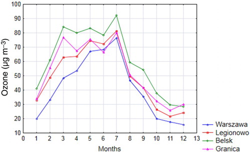
Fig. 1 Time series of average monthly surface ozone concentration for 2005–2010.

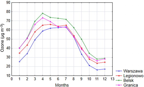
The monthly means of ground level ozone ranged from 16.4 µg m⁻³ to 78.2 µg m⁻³. A seasonal maximum occurs in spring and early summer (April, May, June, and July). Additionally, in Granica high values are also recorded in March. The highest ozone concentrations are found at rural stations (Granica and Belsk) in April (73.5 and 78.2 µg m⁻³, respectively). At the suburban (Legionowo) and urban (Warszawa) stations maximum concentrations are 66.3 µg m⁻³ (May) and 63.6 µg m⁻³ (July), respectively. A seasonal minimum occurs in autumn and early winter (October, November, and December). The lowest values are recorded in November at the urban (Warszawa) and suburban (Legionowo) stations (16.4 and 23.6 µg m⁻³, respectively). At rural stations (Granica and Belsk) these concentrations are 26.2 and 28.1 µg m⁻³, respectively. Despite the fact that the stations are located close to each other, different concentrations of surface ozone are observed.

The spring maximum in surface ozone concentration at the stations studied is commonly observed at many sites in the northern hemisphere (Monks, 2000 and references therein). Wang, Jacob, and Logan (1998) demonstrated that the phenomenon of an ozone maximum in April is caused by two factors: stratospheric–troposheric exchange (most intense from January to April) and ozone formation processes in the troposhere which are observed to peak in April to June. They proved that the occurrence of a broad spring–summer ozone maximum at urban stations indicates that photochemical processes within the lower troposphere are the dominant source of surface ozone. It can be concluded that the autumn–winter ozone minimum results from limited photochemical ozone production and scarce stratospheric–tropospheric exchange events.

b Diurnal Variations in Surface Ozone

Diurnal variations in ozone concentration provide us with an easier understanding of processes responsible for the formation and destruction of surface ozone at a particular place (Elampari & Chithambarathanu, 2011).

Figures 2 and 3 present the average diurnal variations in ozone in July and January for all stations studied.

Fig. 2 Time series of average diurnal surface ozone concentration for July 2005–2010.

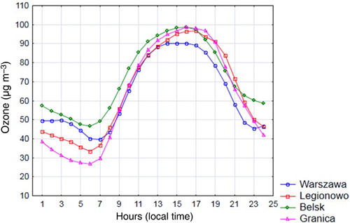
Fig. 3 Time series of average diurnal surface ozone concentration for January 2005–2010.

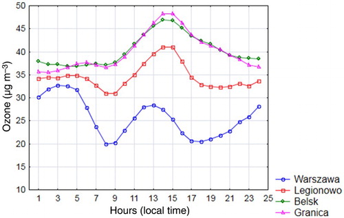
The distribution of ozone concentration in the summer is completely different from that in winter. Ozone concentration at all stations in July show that the minimum occurs shortly after sunrise (about 05:00 to 07:00 local time). In the morning hours, surface deposition plays a significant role because of the temperature inversion (Tarasova & Karpetchko, 2003). Probably the location of the Granica station in a forested area results in enhanced dry deposition processes causing the lowest values of the diurnal minimum to occur there. Relatively clear minima during the early morning hours at Warszawa and Legionowo stations are typical for urban areas (Tu, Xia, Wang, & Li, 2007). From 07:00 local time, coinciding with increasing solar radiation and temperature, the amount of ozone increases to reach a maximum in the afternoon (13:00–17:00 local time). High ozone concentrations during daytime is additionally the result of mixing processes in the boundary layer (Lal, Naja, & Subbaraya, 2000). Heating of the Earth's surface induces convection processes that mix pollutants. Furthermore, higher altitude ozone-rich air is mixed with ozone-poor air near the ground. In January we observed a different diurnal ozone distribution depending on the station type. At rural stations higher concentrations occur between 11:00 and 19:00 local time with a maximum (about 47 µg m⁻³) from 14:00 to 15:00 local time whereas during the rest of the day ozone concentration remains very stable (36–40 µg m⁻³). At urban and suburban stations we noted two clear minima at about 08:00 and 17:00–18:00 local time. In cities this situation is probably related to rush hours and increased production of NO. Nitrogen oxide reacts with ozone leading to the formation of most nitrogen dioxide in the atmosphere as shown by the following reaction (Crutzen et al., 1999).

c Frequency Distribution of Surface Ozone Concentration

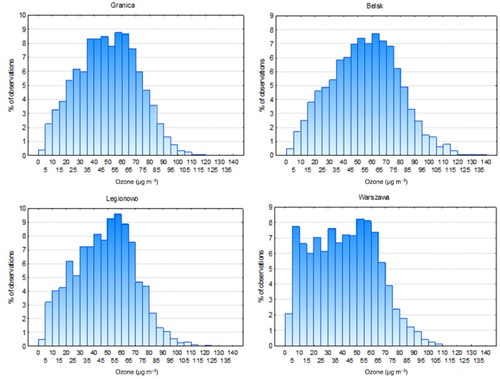
Figure 4 shows the frequency distribution for surface ozone at all stations studied. At the rural station in Granica about 60% of all measurements were between 35 and 70 µg m⁻³; at Belsk, the second rural station, about 60% of measurements were between 35 and 80 µg m⁻³. At the suburban station, Legionowo, about 60% of all measurements were between 30 and 70 µg m⁻³. At the urban station in Warszawa we observed a completely different distribution pattern of surface ozone concentration, about 90% of the observations were between 5 and 70 µg m⁻³. At rural stations Granica and Belsk 25% and 23%, respectively, of all measurements were between 0 and 35 µg m⁻³. At the suburban in Legionowo 25% of the measurements were between 0 and 30 µg m⁻³, and at the urban in Warszawa 2% of the measurements were between 0 and 5 µg m⁻³. About 15% of the measurements at the Granica station were above 70 µg m⁻³, and about 15% at the Belsk station were above 80 µg m⁻³. At the suburban and urban stations measurements over 70 µg m⁻³ occurred 15% and 8% of the time, respectively. In conclusion, when comparing results from all the stations under investigation, a higher percentage of measurements of low ozone concentration (below 30 µg m⁻³) was noticed at the urban station (Warszawa).

Fig. 4 Frequency distribution of surface ozone concentration for the 2005–2010 time series.

d Analysis of Ozone Episodes

Surface ozone present in the ambient air is one of the most harmful air pollutants. Longer exposure at high ozone concentrations may have noxious effects including changes in lung capacity, epithelial permeability, or flow resistance which can be observed even many days after the exposure event. Repeated exposure may exacerbate some of above effects (Holton, Curry, & Pyle, 2003). In order to protect human health the European Parliament, Council of the European Union (2008) established a target value of 120 µg m⁻³ for the maximum daily 8-hour mean of surface ozone. The threshold at a given station is exceeded when the target value is exceeded 25 times in the 3-year average.

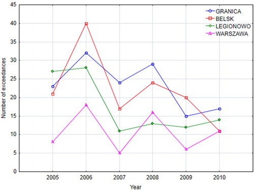
Figure 5 shows the time series of the number of days in a year when surface ozone exceeded the threshold value (120 µg m⁻³ per 8 h) at all stations from 2005 to 2010. Statistical analysis of 8-hourly averaged data exhibits a significant number of days exceeding (above 120 µg m⁻³) the long-term target value set for ozone during the period under study (2005–2010). Ozone levels above 120 µg m⁻³ occurred in every year analyzed from March to September. High ozone events were observed more frequently at rural sites (Belsk and Granica) than at urban stations (Warszawa and Legionowo). Analysis of year-to-year variability demonstrates that the number of days with elevated ozone concentration levels since 2006 shows a downward tendency with the exception of Warszawa station where no observable tendency is noticed (Fig. 5). During the period analyzed the long-term limit set for surface ozone to protect human health (values above 120 µg m⁻³ per 8 h more than 25 times in a 3-year average) was exceeded at both rural stations for the 3-year periods 2005, 2006, and 2007 as well as 2006, 2007, and 2008. The number of exceedances during the 3-year periods at the Belsk station were 26 and 27, respectively, whereas at the Granica station the number of exceedances were 26 and 28, respectively. At urban stations there was no such situation.

Fig. 5 Number of days when ozone concentrations exceeds 120 µg m⁻³ per 8 h in a year.

Very high levels of surface ozone concentration (above 180 µg m⁻³) were noticed only during two of (2005 and 2006) the six years analyzed (2005–2010). The alarm threshold (above 240 µg m⁻³) was not exceeded during the period of analysis.

Both local and remote sources of surface ozone are responsible for the concentration at a given location. Backward trajectory modelling is a useful tool for estimating the possible atmospheric transport to one of the stations under study. In fact, it is possible to determine the path of the air parcels and the area from where the pollution is transported.

To determine atmospheric transport pathways connected with elevated ozone concentrations, the 72-hour backward trajectories arriving at the sites studied during 2005–2010 were clustered into six sectors. For this purpose the Hybrid Single-Particle Lagrangian Integrated Trajectory (HYSPLIT) model developed by the National Oceanic and Atmospheric Administration (NOAA) Air Resources Laboratory was used. Trajectories (500, 1000, and 1500 m above ground level were plotted for each day when the long-term target value for surface-level ozone was exceeded. The distribution of defined trajectories (number and percentage) for the stations studied is presented in Table 3.

Table 3. Summary statistics of trajectories arriving at analyzed stations in 2005–2010 by sectors, pathways and air masses of atmospheric transport.

Sector	Air mass	Pathway	Number	Percentage
				Belsk	Granica	Legionowo	Warszawa
North	AA	SC→BS	25	8	11	6	9
Northwest	AA	UK→NS→D→BS	32	15	9	9	12
West	MPA	AO→F→BC→G	33	9	14	12	12
Southwest	TMA	S→F→G	82	32	25	31	28
East	CPA	B/U→R	76	26	29	28	21
S	TCA	Ro→H→Sl	37	9	12	14	18

Air masses: AA-Arctic, MPA-Maritime polar, TMA-Tropical maritime, CPA-Continental polar, TCA-Tropical continental.

Pathway: SC-Scandinavian countries, UK-United Kingdom, NS-North Sea, D-Denmark, BS-Baltic Sea, AO-Atlantic Ocean, F-France, BC-Benelux countries, G-Germany S-Spain, B-Belarus, U-Ukraine, R-Russia, Ro-Romania, H-Hungary, Sl-Slovakia.

The percentage distribution of defined trajectories was similar at each station. The Southwest and East sectors dominate the others (29% and 26%, respectively). These sectors are associated with a tropical maritime air mass and a continental polar air mass, respectively. The first air mass flows in from the Azores bringing warm, humid air during the summer characterized by hot, sultry weather. The second air mass originates in the temperate latitudes of Europe and Asia. In Poland during warm months this air mass is characterized by sunny, hot, dry weather with frequent thermal convection. The South sector has a significantly lower percentage (14%). Atmospheric transport from the Northwest and West sectors represents 11% and 12%, respectively. The smallest number of trajectories was associated with the North sector (8%). Many trajectories (about 30%) were excluded from the analysis and assigned to an unidentified class because of the complex structure of the circulation over Poland. It is worth mentioning that high ozone episodes were most often associated with trajectories passing over inland sectors (Southwest and East) rather than over water areas (the Baltic or North Sea and the Atlantic Ocean). Continental air masses are probably more polluted than maritime air masses and are thus responsible for the high ozone concentration in the areas affected by them.

Episodes of high surface ozone concentration lasted 1, 2, 3, 4, 5, 6, 8, and 9 days. About 56% of all episodes at all stations lasted only 1 day, 25% lasted 2 days, 10% lasted 3 days, 5% lasted 4 days, 2% lasted 5 days, and about 2% of the episodes lasted 6, 8, or 9 days. The longest continuous period of surface ozone concentration above 120 µg m⁻³ at any of the stations studied occurred in July 2006 and lasted for 6 days at Warszawa and 9 days at Legionowo. Meteorological conditions during this period were favourable for photochemical ozone production (temperature of 30°C, relative humidity below 50%, intense solar radiation, and wind speed usually below 3 m s⁻¹). Of all the years analyzed, 2006 was unique in this study, in terms of high monthly average concentrations of surface ozone (Fig. 6). During 2006 the highest ozone concentrations were recorded in July, in particular at the rural station in Belsk (above 90 µg m⁻³) but also the other stations had high concentrations (up to 80 µg m⁻³). Quite high values of surface ozone concentrations lasted continuously from March to June (60–85 µg m⁻³) at the suburban and rural stations. Most likely, favourable weather conditions in 2006 created optimal conditions for ozone formation causing the highest number of exceedances of the target value of 120 µg m⁻³ during the period under study.

Fig. 6 Monthly averaged surface ozone concentration for the 2006 time series.

e Ozone “Weekend Effect”

The primary cause of higher surface ozone concentrations during weekends is most likely the result of a reduction in NO_x emissions in a VOC-limited regime (Heuss et al., 2013). At low VOC:NO_x ratios, OH radicals usually react with NO₂ inhibiting O₃ formation: OH + NO₂ + M → HNO₃ + M. If the emission of NO_x is limited, which is the case during weekends, OH radicals preferentially react with VOC molecules initiating production of O₃ (Fujita et al., 2013). The second, equally important, hypothesis to explain the cause of the ozone weekend effect is the “ozone quenching hypothesis”, which is based on the process of ozone titration by NO. Lower emissions of NO during weekends reduces the mechanism of ozone destruction: NO + O₃ → NO₂ + O₂ (Sadanaga, Sengen, Takenaka, & Bandow, 2012).

To determine the weekly pattern of surface ozone concentration and explore the weekend effect phenomenon, surface ozone and NO₂ data from January 2005 to December 2010 (measured at Granica, Belsk, Legionowo, and Warszawa stations) were investigated in terms of a weekly cycle. The average means of O₃ and NO₂, by day of week, for each station are presented in Table 4.

Table 4. Daily averaged concentration for the 2005–2010 time series of O₃ and NO₂. Numbers in bold indicate the highest values during the week; numbers in bold italic font indicate the lowest values during the week.

2005–2010	Granica		Belsk		Legionowo		Warszawa
	O3 (µg m^−3)	NO2 (µg m^−3)	O3 (µg m^−3)	NO2 (µg m^−3)	O3 (µg m^−3)	NO2 (µg m^−3)	O3 (µg m^−3)	NO2 (µg m^−3)
Monday	50.02	8.61	55.47	10.11	47.58	19.20	40.99	28.46
Tuesday	48.94	9.66	53.86	11.40	46.81	20.47	39.40	29.27
Wednesday	48.61	9.49	53.85	11.24	46.79	19.18	39.05	29.19
Thursday	49.83	9.47	54.23	11.33	47.25	19.20	39.84	28.86
Friday	48.99	9.67	54.33	11.48	46.91	19.66	39.26	28.81
Saturday	51.02	8.39	55.91	9.98	49.53	16.93	45.01	23.57
Sunday	51.70	7.07	56.86	8.19	50.80	14.89	47.55	20.46
Wd	49.28	9.38	54.35	11.11	47.07	19.54	39.71	28.92
Sa–Su	51.36	7.73	56.39	9.09	50.16	15.91	46.28	22.02

Wd-weekday daily mean concentrations, Sa–Su-weekend daily mean concentrations.

At all stations surface ozone concentrations were higher on weekends than on weekdays, albeit at the background stations (Granica and Belsk) the high amounts remained elevated on Mondays. The highest values were reached on Sundays and the lowest on Wednesdays. Although the general pattern at each station is similar, the values of the daily means were significantly different. During weekdays mean concentrations ranged from 39.71 µg m⁻³ (Warszawa) to 54.35 µg m⁻³ (Belsk) and during weekends from 46.28 µg m⁻³ (Warszawa) to 56.39 µg m⁻³ (Belsk). At the background stations, Granica and Belsk, the differences between mean concentrations during weekends and weekdays were 2.08 µg m⁻³ and 2.04 µg m⁻³, respectively, and in Legionowo and Warszawa they were 3.09 µg m⁻³ and 6.57 µg m⁻³, respectively. Weekly cycles of NO₂ reveal higher concentrations on weekdays than on weekends; hence, the variations were the opposite to those of surface ozone. At all stations, the lowest concentrations of NO₂ in the weekly cycle were noticed on Sundays. The highest concentrations occur with some consistency: at the background stations (Granica and Belsk) the highest concentrations occurred on Fridays and at the suburban and urban stations (Legionowo and Warszawa) on Tuesdays. During weekdays, concentrations ranged from 9.38 µg m⁻³ (Granica) to 28.92 µg m⁻³ (Warszawa) and during weekends from 7.74 µg m⁻³ (Granica) to 22.02 µg m⁻³ (Warszawa). At the background stations, Granica and Belsk, the differences between mean concentrations during weekdays and weekends were 1.65 µg m⁻³ and 2.02 µg m⁻³, respectively and were 3.63 µg m⁻³ at Legionowo and 6.90 µg m⁻³ at Warszawa. The differences between weekday and weekend surface ozone and NO₂ concentrations at all stations were statistically significant.

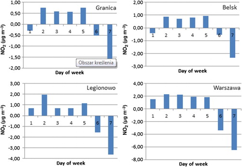
The differences from the daily average ozone and NO₂ concentrations for the 2005–2010 time series are presented in Figs 7 and 8. Positive deviations in ozone, relative to the average for 2005–2010, were noticed on Saturday, Sunday, and Monday at the background stations (Granica and Belsk). Positive deviations in NO₂ were noticed during weekdays (except Monday at the background stations). As described above, this contrasting pattern confirms the non-linear relationship between NO_x and O₃. Furthermore, it indicates the close linkages between a reduction in NO₂ emissions on weekends and a higher concentration of O₃. Higher values of the differences at suburban and urban stations reveal that the weekend effect is predominantly a phenomenon of large cities where a VOC-limited chemical regime prevails.

Fig. 7 Surface ozone concentrations relative to the average for the 2005–2010 time series where 1 means Monday and 7 Sunday.

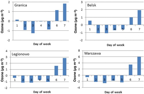
Fig. 8 Nitrogen dioxide concentrations relative to the average for the 2005–2010 time series where 1 means Monday and 7 Sunday.

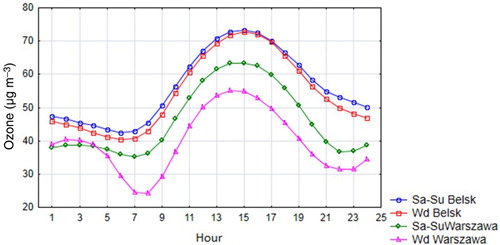
Two different types of stations, an urban (Warszawa) and a background (Belsk), were chosen to illustrate the diurnal cycles of surface ozone during weekends and weekdays (Fig. 9). The first conspicuous difference is an almost imperceptible ozone weekend effect at the rural station because of the small variability in NO_x in the weekly cycle (Melkonyan & Kuttler, 2012). Slightly higher values of ozone concentration during weekends were noted only during the nighttime, hours which can be caused by smaller amounts of NO and, hence, weakened ozone titration processes (Melkonyan & Kuttler, 2012).

Fig. 9 Diurnal and weekly cycles of surface ozone at an urban (Warszawa) station and a background (Belsk) station for the 2005–2010 time series. Sa-Su: weekend, Wd-weekdays.

To determine which of the hypotheses mentioned previously is responsible for the occurrence of the ozone weekend effect, the concentration of the “oxidant” (O_x), which represents the sum of NO₂ and O₃ (Itano et al., 2007), at stations Warszawa and Belsk was calculated. The O_x are important indicators in analyzing the “ozone quenching” hypothesis because the concentration of O_x is preserved in the titration of ozone by NO: NO + O₃ → NO₂ + O₂. If the “ozone quenching” assumption is the main cause of the ozone weekend effect then the concentration of O_x would be approximately the same during weekends and weekdays (Sadanaga et al., 2012). As presented in Table 5, concentrations of O_x were approximately the same. The difference at the urban station was 0.67 µg m⁻³, and at the background station it was 0.22 µg m⁻³. This means that photochemical ozone production occurs during weekends but ozone titration processes by NO due to reduced emission are limited. Finally smaller amounts of O₃ are destroyed during weekends.

Table 5. Average concentration during weekdays and weekends for the 2005–2010 time series of O_x.

	Warszawa		Belsk
	Weekdays (µg m^−3)	Weekends (µg m^−3)	Weekdays (µg m^−3)	Weekends (µg m^−3)
2005	66.82	68.29	65.96	65.78
2006	72.43	72.58	72.50	73.72
2007	65.92	64.84	61.56	61.92
2008	68.07	67.75	64.73	64.77
2009	69.65	66.09	63.31	60.06
2010	–	–	64.61	65.16
Average (2005–2010)	68.58	67.91	65.45	65.23

f Influence of Meteorological Parameters on Surface Ozone Concentration

Determination of the effect of meteorological parameters on surface ozone concentration and its precursors at a given place enables a better understanding of regional and local causes of surface ozone pollution. Temperature at 2 m, total solar radiation, relative humidity, pressure, wind speed, and V and U wind velocity components were chosen to investigate the influence of local meteorological parameters on surface ozone concentration. Most processes responsible for photochemical formation, transport, and deposition of ozone can be parameterized by these meteorological parameters. In this analysis ozone concentrations are defined as the average amount of surface ozone measured between sunrise and sunset (i.e., from 07:00 to 20:00 summer local time (utc + 2 h) and between 08:00 and 16:00 winter local time (utc+1 h)). The same approach was applied for all meteorological parameters. In Table 6 the matrix of the correlation coefficients between surface ozone and the meteorological parameters for Belsk and Warszawa (to determine the differences between urban and rural stations) in summer and winter are presented.

Table 6. Correlation coefficients for seasonal mean surface ozone and meteorological parameters. The statistically significant coefficients at the 95% confidence level are in bold font. The 2010 coefficients for Warszawa were not calculated because the NO₂ data for Warszawa were missing (required to calculate O_x). Pressure data for Warszawa station are missing.

Belsk Summer	2005	2006	2007	2008	2009	2010	Belsk Winter	2005	2006	2007	2008	2009	2010
T	0.66	0.77	0.71	0.5	0.4	0.77	T	−0.27	−0.1	−0.23	0.33	−0.27	−0.03
RH	−0.36	−0.72	−0.61	−0.68	−0.51	−0.75	RH	−0.45	−0.4	−0.61	−0.71	−0.59	−0.54
SR	0.54	0.68	0.6	0.62	0.57	0.74	SR	0.5	0.66	0.39	0.51	0.59	0.74
P	0.16	0.48	0.06	0.13	−0.01	0.26	P	−0.09	−0.04	−0.07	−0.19	0.25	−0.27
WS	−0.27	−0.28	−0.17	−0.06	−0.12	−0.25	WS	0.21	0.08	0.45	0.61	0.2	0.28
V	−0.11	0.13	0.26	−0.09	−0.14	−0.07	V	0.13	−0.07	0.01	0.21	−0.08	0.08
U	0.08	0.09	−0.03	−0.03	0.21	−0.14	U	−0.12	0.17	−0.04	−0.12	−0.02	−0.12
Warszawa Summer	2005	2006	2007	2008	2009	2010	Warszawa Winter	2005	2006	2007	2008	2009	2010
T	0.66	0.77	0.85	0.58	0.5	—	T	−0.34	−0.18	−0.3	−0.11	−0.28	—
RH	−0.61	−0.7	—	—	—	—	RH	−0.52	−0.27	−0.58	—	—	—
SR	0.64	0.66	0.88	0.67	0.42	—	SR	0.64	0.48	0.52	0.34	0.45	—
WS	−0.07	−0.22	−0.08	0.04	0.02	—	WS	0.47	0.18	0.49	0.65	0.33	—
V	0.11	−0.05	0.27	−0.25	−0.11	—	V	−0.13	0.00	0.04	0.09	−0.13	—
U	0.11	0.2	−0.31	0.08	0.13	—	U	0.05	0.04	−0.05	0.1	−0.02	—

T-temperature, RH-relative humidity, SR-solar radiation, P-pressure, WS-wind speed, V and U are the vertical and horizontal components of the wind, respectively.

The values of the correlation coefficients clearly depend more on the season than the location. During summer, at both stations, the correlation with temperature was always statistically significant and positive, ranging from 0.40 to 0.85. Temperature is an important meteorological parameter that controls ozone formation. Higher temperature causes increased emission of VOCs especially isoprene, which play a significant role in ozone production (Bell & Ellis, 2004). During winter the coefficients were, in almost all cases, negative; 36% were statistically insignificant and ranged from −0.03 to −0.34. The explanation for this is that Arctic air masses coming from the north are rich in ozone. During winter these air masses contribute to a decrease in temperature while simultaneously increasing surface ozone concentration. The correlation with solar radiation was positive during both seasons with the values being higher in summer (0.42–0.88) than in winter (0.34–0.74). Solar radiation is the main meteorological parameter involved in photochemical reactions (Ordóñez et al., 2005). Solar radiation is an essential factor in NO₂ photolysis (source of surface ozone):

The correlation of surface ozone with relative humidity was negative and statistically significant in all cases and ranged from −0.36 to −0.75 during summer and from −0.27 to −0.71 during winter. On a molecular level ozone and water vapour are involved in a chain of reactions:

where O(¹D) is an oxygen atom in the excited state

where O(³P) is an oxygen atom in an ground state

In the first set of reactions, the excited atom (O(¹D)) reacts with water vapour to create OH radicals. In the second set of reactions, collision with another molecule (M) forms ozone. Hence, we can deduce the importance of water vapour in the air to ozone concentration. The higher the number of water molecules in the air the higher the probability of OH creation and less ozone formation. On the other hand, according to Chan et al. (2003) the relationship between high ozone values and low relative humidity might result from the transport of upper tropospheric air which is dry and abundant in ozone. In accordance with Nishanth, Praseed, Satheesh Kumar, and Valsaraj (2012) higher values of humidity are usually associated with extensive cloud cover and atmospheric instability. Probably as a result of limited solar radiation photochemical ozone formation is slowed down. The correlation of surface ozone with wind speed during summer in most cases is negative with low values (maximum −0.28), whereas during winter the coefficients were positive and reached a maximum of 0.65. It is possible that during winter, when photochemical reactions are reduced, long-range transport contributes to surface ozone concentration. Higher wind speeds result in faster transport and atmospheric mixing, in effect increasing ozone concentration (Tu et al., 2007). Pressure and the V and U components of the wind do not play a significant role in surface ozone formation which is shown by the low correlation coefficients which are, for the most part, statistically insignificant.

g Results of the Multiple Regression Model

A multiple regression model was used to determine how surface ozone concentration depends on standard meteorological parameters. The analysis was performed using the Statistica statistical software, version 10. Forward and backward stepwise regression models were performed for the rural (Belsk) and urban (Warszawa) stations, separately for summer and winter, using about 90 daily (7:00–20:00 local time in summer and 8.00–16.00 local time in winter) data points each year. Initially, meteorological parameters (temperature, solar radiation, wind speed, V, and U) for the entire analysis time (2005–2010) were included in the input to the model on the assumption that they are important to ozone variability. Finally, the stepwise regression model provided only variables which significantly (at the 0.05 significance level) affect the model output (Table 7). For each station analyzed, separately for summer (2005–2010) and winter (2005–2010), the following parameters were found to be statistically significant: (1) Belsk summer: temperature and solar radiation; (2) Belsk winter: temperature, solar radiation, and wind speed; (3) Warszawa summer: temperature and solar radiation; and (4) Warszawa winter: temperature, solar radiation, and wind speed.

Table 7. Results of the multiple regression model for O₃ for Belsk and Warszawa stations in winter and summer from 2005 to 2010. R is the correlation coefficient; R² is the coefficient of determination.

	Belsk 2005–2010			Warszawa 2005–2010
Stepwise Regression	R	R^2	Parameters	R	R^2	Parameters
Summer
forward	0.73	0.53	temperature	0.75	0.56	temperature
			solar radiation			solar radiation
backward	0.73	0.53	temperature	0.75	0.56	temperature
			solar radiation			solar radiation
Winter
forward	0.65	0.41	temperature	0.65	0.41	temperature
			solar radiation			solar radiation
			wind speed			wind speed
backward	0.65	0.41	temperature	0.65	0.41	temperature
			solar radiation			solar radiation
			wind speed			wind speed

Then, using cross-validation, prediction scores were estimated. One year was reserved for model testing; the remaining years were used for model training, and prediction scores were calculated using the test data. This process was repeated until all years were used for testing. The values of the correlation coefficients between the predicted and observed ozone concentrations are presented in Table 8.

Table 8. Correlation coefficients between the predicted and observed ozone concentrations.

	Belsk		Warszawa
	R		R
	Summer	Winter	Summer	Winter
2005	0.57	0.50	0.73	0.66
2006	0.61	0.67	0.67	0.49
2007	0.67	0.40	0.88	0.54
2008	0.63	0.52	0.68	0.35
2009	0.57	0.60	0.44	0.47
2010	0.76	0.74	–	–

Temperature and solar radiation proved to be the most important meteorological parameters at both stations. The coefficient of determination was 0.56, which means that up to 56% of O₃ total daily variation during summer can be accounted for using temperature and solar radiation. During winter, wind speed is also statistically important and together with temperature and solar radiation can explain up to 41% of O₃ daily concentration at both stations. Considerably lower coefficients during winter are evidence that these parameters contribute less to the formation of in situ ozone (probably because of limited solar radiation) and that dynamic processes make the dominant contribution to the transport of ozone from remote areas (this is also indicated by the statistically significant influence of wind speed on ozone variability).

h Results of the Multilayer Perceptron Neural Network Artificial Model

In recent years the multilayer perceptron (MLP) neural network system has been widely used to estimate the concentration of air pollutants. The advantage of this type of model is the possibility of capturing complicated, non-linear relationships between the concentration of predictors and the values of meteorological parameters (Gardner & Dorling, 2000). In this work a three-layer network (with a single hidden layer) was used to predict surface ozone concentration using basic meteorological parameters and the concentration of NO₂ (using the Statistica neural network commercial package).

In this study three meteorological parameters, daily average values of temperature, relative humidity, and solar radiation from 07:00 to 20:00 local time were used to define the meteorological regime during summer, and four parameters, daily average values of temperature, relative humidity, solar radiation, and wind speed from 08:00 to 16:00 local time were used to define the meteorological regime during winter (the use of wind speed significantly improved the outcome of the model). Meteorological data and NO₂ concentration covered the six-year period from 2005 to 2010. Summer and winter data were divided into three separate and equally representative measuring period datasets: training, validation, and testing. During the process of network training the fitting error in the testing set was continuously tracked. In order to avoid overfitting, when the test error stopped decreasing the early stopping method was used. To optimize the final results, about 250 neural networks were trained and analyzed but only those with the lowest error values and the highest correlation coefficients were chosen for further analysis. The number of parameters was determined by the number of meteorological variables. During the process of network training the most significant parameters were selected with the final number being a maximum of 8 and a minimum of 4. The number of neurons in the hidden layer varied from 4 to 8 depending on the case (rural-urban, summer-winter).

The results from the MLP neural network on the basis of the validation dataset (an independent dataset not involved in the process of network training) are presented in Table 9.

Table 9. Results from the MLP neural network for summer and winter from 2005 to 2010 for Belsk and Warszawa stations.

	Correlation Coefficient	Average Deviation (%)	Standard Deviation (%)
Belsk summer	0.84	−6.8	15
Belsk winter	0.78	−3.7	27
Warszawa summer	0.89	0.6	19
Warszawa winter	0.83	−9.8	36

Table 9 shows that using the MLP neural network tool with basic meteorological parameters and the NO₂ concentration we are able to estimate the average daily surface ozone concentration with very high accuracy. The correlation coefficients were 0.84 (Belsk) and 0.89 (Warszawa) for summer and 0.78 (Belsk) and 0.83 (Warszawa) for winter. The larger deviations during winter are caused by the lower surface ozone concentration in the winter months. Because the network works with approximately the same absolute error (from 6 to 8.8 µg m⁻³) in winter the relative error is larger.

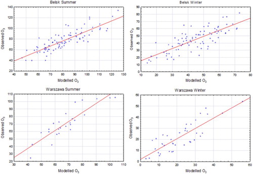
Figure 10 presents the comparison between measured values of surface ozone and estimated values using the MLP neural network model. There is better correlation between measured and modelled concentrations in summer at both locations. The correlation coefficients were 0.84 and 0.89 for Warszawa and Belsk stations, respectively. Slightly poorer agreement occurs during winter; correlation coefficients were 0.78 for Belsk and 0.83 for Warszawa stations. This suggests that during winter, photochemical processes which lead to ozone formation play a less important role than in summer. It is probable that the variability of surface ozone is mostly governed by dynamical processes during winter.

Fig. 10 Comparison of measured and estimated values of O₃ for Belsk and Warszawa stations during summer and winter.

5 Conclusions

Simultaneous measurements of surface ozone and standard meteorological parameters were performed from 2005 to 2010 for four different types of stations located in the central region of Poland. The analysis was performed in terms of diurnal, monthly, and seasonal cycles.

The results from measurements show that the concentration of surface ozone is higher at rural locations than at urban or suburban locations. At locations where traffic flow is greater, chemical reactions involving surface ozone and nitrogen oxides to produce oxygen and nitrogen dioxide are common. From diurnal averages it was found that the lowest ozone concentration occurs in the early morning hours and the maximum in the afternoon hours. The seasonal ozone maximum occurs in spring and early summer and the minimum in autumn.

Days with surface ozone concentration above 120 µg m⁻³ per 8 h were recorded in each year during the measurement period (2005–2010) from March to September, usually at rural stations. The highest number of such days was noticed in 2006 as a result of specific meteorological conditions in Europe (sunny weather, advection of hot dry air, and numerous thermal inversions). Since 2008 there has been a decreasing trend in the number of days with high ozone concentration at all locations studied except at Warszawa station.

Ozone concentrations differ significantly on weekend days and weekdays. Concentrations are higher during the weekend because of limited processes for ozone titration by NO. Results of multiple regression and MLP neural network models confirmed that meteorological parameters, especially temperature, solar radiation, and relative humidity could explain a significant amount of surface ozone variability.

The results of this work advances our knowledge of surface ozone distribution over the selected sites and also the effect of standard meteorological parameters on ozone concentration. However, further parameterization of dynamical processes, especially the transport of ozone and its precursors to the Mazowieckie voivodeship are necessary to understand the variability of surface ozone in this area.

Acknowledgements

This work was partially supported by the Regional Inspectorate of Environmental Protection in Warsaw and partially performed under statutory activity No: 3841/E-41/S/2014 of the Minister of Science and Higher Education in Poland. We appreciate the comments and suggestions of anonymous reviewers, which significantly improved our manuscript.

References

- An, D. D., Co, H. X., & Kim Oanh, N. T. (2008). Photochemical smog introduction and episode selection for the ground-level ozone in Hanoi, Vietnam. VNU Journal of Science, Earth Sciences, 24, 169–175.
- Bell, M., & Ellis, H. (2004). Sensitivity analysis of tropospheric ozone to modified biogenic emissions for the mid-Atlantic region. Atmospheric Environment, 38, 1879–1889. doi: 10.1016/j.atmosenv.2004.01.012
- Blum, O., & Didyk, N. (2007). Study of ambient ozone phytotoxicity in Ukraine and ozone protective effect of some antioxidants. Journal of Hazardous Materials, 149, 598–602. doi: 10.1016/j.jhazmat.2007.06.112
- Cape, J. N. (2008). Surface ozone concentrations and ecosystem health: Past trends and a guide to future projections. Science of the Total Environment, 400, 257–269. doi: 10.1016/j.scitotenv.2008.06.025
- Chan, C. Y., Chan, L. Y., Cui, H., Zheng, X. D., Zheng, Y. G., Qin, Y., & Li, Y. S. (2003). Origin of the springtime tropospheric ozone maximum over east China at LinAn in 2001. Tellus, 55B, 982–992. doi: 10.1034/j.1600-0889.2003.00079.x
- Crutzen, P. J., Lawrence, M. G., & Pöschl, U. (1999). On the background photochemistry of tropospheric ozone. Tellus, 51A-B, 123–146.
- Debaje, S. B., & Kakade, A. D. (2009). Surface ozone variability over western Maharashtra, India. Journal of Hazardous Materials, 161, 686–700. doi: 10.1016/j.jhazmat.2008.04.010
- Di Carlo, P., Pitari, G., Mancini, E., Gentile, S., Pichelli, E., & Visconti, G. (2007). Evolution of surface ozone in central Italy based on observations and statistical model. Journal of Geophysical Research, 112, D10316. doi: 10.1029/2006JD007900
- Elampari, K., & Chithambarathanu, T. (2011). Diurnal and seasonal variations in surface ozone levels at tropical semi-urban site, Nagercoil, India, and relationships with meteorological conditions. International Journal of Science and Technology, 1, 80–88.
- European Parliament, Council of the European Union. (2008). Directive 2008/50/EC of the European Parliament and of the Council of 21 May 2008 on ambient air quality and cleaner air for Europe. OJ L 152, 11.6.2008, p. 1–44 (BG, ES, CS, DA, DE, ET, EL, EN, FR, IT, LV, LT, HU, MT, NL, PL, PT, RO, SK, SL, FI, SV).
- Fujita, E. M., Campbell, D. E., Zielinska, B., Sagebiel, J. C., Bowen, J. L., Goliff, W. S., … Lawson, D. R. (2013). Diurnal and weekday variations in the source contributions of ozone precursors in California's South Coast Air Basin. Journal of the Air & Waste Management Association, 53(7), 844–863. doi: 10.1080/10473289.2003.10466226
- Gardner, M. W., & Dorling, S. R. (2000). Meteorologically adjusted trends in UK daily maximum surface ozone concentrations. Atmospheric Environment, 34, 171–176. doi: 10.1016/S1352-2310(99)00315-5
- Helmig, D., Oltmans, S. J., Carlson, D., Lamarque, J. F., Jones, A., Labuschagne, C., … Hayden, K. (2007). A review of surface ozone in the polar regions. Atmospheric Environment, 41, 5138–5161. doi: 10.1016/j.atmosenv.2006.09.053
- Heuss, J. M., Kahlbaum, D. F., & Wolff, G. T. (2013). Weekday/weekend ozone differences: What can we learn from them? Journal of the Air & Waste Management Association, 53, 772–788. doi: 10.1080/10473289.2003.10466227
- Holton, J. R., Curry, J. A., & Pyle, J. A. (Eds). (2003). Encyclopedia of atmospheric sciences (Vol. 4, pp. 1655–1663). Amsterdam: Academic Press, An Imprint of Elsevier Science.
- IPCC (Intergovernmental Panel on Climate Change). (2001). Climate change 2001. In J. T. Houghton, Y. Ding, D. J. Griggs, M. Noguer, P. J. van der Linden, X. Dai, K. Maskell, & C. A. Johnson (Eds.). The scientific basis, contribution of Working Group 1 to the third assessment report. Cambridge, United Kingdom and New York, NY, USA: Cambridge University Press.
- Isaksen, I. S. A. (2003). Ozone-climate interactions. EC, Brussels, Belgium: Air Pollution Research Report No. 81.
- Itano, Y., Bandow, H., Takenaka, N., Saitoh, Y., Asayama, A., & Fukuyama, J. (2007). Impact of NOx reduction on long-term ozone trends in an urban atmosphere. Science of the Total Environment, 379, 46–55. doi: 10.1016/j.scitotenv.2007.01.079
- Kalabokas, P. D., & Repapis, C. C. (2004). A climatological study of rural surface ozone in central Greece. Atmospheric Chemistry and Physics, 4, 1139–1147. doi: 10.5194/acp-4-1139-2004
- Kulkari, P. S., Bortoli, D., Salgado, R., Antón, M., Costa, M. J., & Silva, A. M. (2011). Tropospheric ozone variability over the Italian Peninsula. Atmospheric Environment, 45, 174–182. doi: 10.1016/j.atmosenv.2010.09.029
- Lal, S., Naja, M., & Subbaraya, B. H. (2000). Seasonal variations in surface ozone and its precursors over an urban site in India. Atmospheric Environment, 34, 2713–2724. doi: 10.1016/S1352-2310(99)00510-5
- Lazutin, L., Bezerra, P. C., Fagnani, M. A., Pinto, H. S., Martin, I. M., Da Silva, E. L. P., … Zullo, J. R. J. (1996). Surface ozone study in Campinas, Sao Paulo, Brazil. Atmospheric Environment, 30, 2729–2738. doi: 10.1016/1352-2310(95)00280-4
- Logan, J. A. (1985). Tropospheric ozone: Seasonal behavior, trends and anthropogenic influence. Journal of Geophysical Research, 90, 10463–10482. doi: 10.1029/JD090iD06p10463
- Melkonyan, A., & Kuttler, W. (2012). Long-term analysis of NO, NO2 and O3 concentrations in North Rhine-Westphalia, Germany. Atmospheric Environment, 60, 316–326. doi: 10.1016/j.atmosenv.2012.06.048
- Monks, P. S. (2000). A review of the observations and origins of the spring ozone maximum. Atmospheric Environment, 34, 3545–3561. doi: 10.1016/S1352-2310(00)00129-1
- Nishanth, T., Praseed, K. M., Satheesh Kumar, M. K., & Valsaraj, K. T. (2012). Analysis of ground level O3 and NOx measured at Kannur, India. Journal of Earth Science & Climatic Change, 3, 111. doi: 10.4172/2157-7617.1000111
- Ordóñez, C., Mathis, H., Furger, M., Henne, S., Hüglin, C., Staehelin, J., & Prévôt, A. S. H. (2005). Changes of daily surface ozone maxima in Switzerland in all seasons from 1992 to 2002 and discussion of summer 2003. Atmospheric Chemistry and Physics, 5, 1187–1203. doi: 10.5194/acp-5-1187-2005
- Prioas, G. T., Larissi, I. K., Moustris, K. P., Nastos, P. T., & Paliatsos, A. G. (2013). Assessment of surface ozone variability in an urban coastal area at the eastern Mediterranean. Global NEST Journal, 15, 163–168.
- Ribas, À., & Peñuelas, J. (2004). Temporal patterns of surface ozone levels in different habitats of the North Western Mediterranean basin. Atmospheric Environment, 38, 985–992. doi: 10.1016/j.atmosenv.2003.10.045
- Sadanaga, Y., Sengen, M., Takenaka, N., & Bandow, H. (2012). Analyses of the ozone weekend effect in Tokyo, Japan: Regime of oxidant (O3+NO2) production. Aerosol and Air Quality Research, 12, 161–168.
- Tarasova, O. A., & Karpetchko, A. Y. (2003). Accounting for local meteorological effects in the ozone time-series of Lovozero (Kola Peninsula). Atmospheric Chemistry and Physics, 3, 941–949. doi: 10.5194/acp-3-941-2003
- Tripathi, O. P., Jennings, S. G., O'Dowd, C., O'Leary, B., Lambkin, K., Moran, E., … Spain, T. G. (2012). An assessment of the surface ozone trend in Ireland relevant to air pollution and environmental protection. Atmospheric Pollution Research, 3, 341–351.
- Tu, J., Xia, Z. O., Wang, H., & Li, W. (2007). Temporal variations in surface ozone and its precursors and meteorological effects at an urban site in China. Atmospheric Research, 85, 310–337. doi: 10.1016/j.atmosres.2007.02.003
- Wang, Y., Jacob, D. J., & Logan, J. A. (1998). Global simulation of tropospheric O3-NOx-hydrocarbon chemistry: 3. Origin of tropospheric ozone and effects of nonmethane hydrocarbons. Journal of Geophysical Research, 103, 10757–10767. doi: 10.1029/98JD00156