Chemistry–Climate Interactions of Stratospheric and Mesospheric Ozone in EMAC Long-Term Simulations with Different Boundary Conditions for CO₂, CH₄, N₂O, and ODS

Abstract

To evaluate future climate change in the middle atmosphere and the chemistry–climate interaction of stratospheric ozone, we performed a long-term simulation from 1960 to 2050 with boundary conditions from the Intergovernmental Panel on Climate Change A1B greenhouse gas scenario and the World Meteorological Organization Ab halogen scenario using the chemistry–climate model ECHAM5/MESSy Atmospheric Chemistry (EMAC). In addition to this standard simulation we performed five sensitivity simulations from 2000 to 2050 using the rerun files of the simulation mentioned above. For these sensitivity simulations we used the same model setup as in the standard simulation but changed the boundary conditions for carbon dioxide (CO₂), methane (CH₄), nitrous oxide (N₂O), and ozone-depleting substances (ODS). In the first sensitivity simulation we fixed the mixing ratios of CO₂, CH₄, and N₂O in the boundary conditions to the amounts for 2000. In each of the four other sensitivity simulations we fixed the boundary conditions of only one of CO₂, CH₄, N₂O, or ODS to the year 2000.

In our model simulations the future evolution of greenhouse gases leads to significant cooling in the stratosphere and mesosphere. Increasing CO₂ mixing ratios make the largest contributions to this radiative cooling, followed by increasing stratospheric CH₄, which also forms additional H₂O in the upper stratosphere and mesosphere. Increasing N₂O mixing ratios makes the smallest contributions to the cooling. The simulated ozone recovery leads to warming of the middle atmosphere.

In the EMAC model the future development of ozone is influenced by several factors. 1) Cooler temperatures lead to an increase in ozone in the upper stratosphere. The strongest contribution to this ozone production is cooling due to increasing CO₂ mixing ratios, followed by increasing CH₄. 2) Decreasing ODS mixing ratios lead to ozone recovery, but the contribution to the total ozone increase in the upper stratosphere is only slightly higher than the contribution of the cooling by greenhouse gases. In the polar lower stratosphere a decrease in ODS is mainly responsible for ozone recovery. 3) Higher NO_x and HO_x mixing ratios due to increased N₂O and CH₄ lead to intensified ozone destruction, primarily in the middle and upper stratosphere, from additional NO_x; in the mesosphere the intensified ozone destruction is caused by additional HO_x. In comparison to the increase in ozone due to decreasing ODS, ozone destruction caused by increased NO_x is of similar importance in some regions, especially in the middle stratosphere. 4) In the stratosphere the enhancement of the Brewer-Dobson circulation leads to a change in ozone transport. In the polar stratosphere increased downwelling leads to additional ozone in the future, especially at high northern latitudes. The dynamical impact on ozone development is higher at some altitudes in the polar stratosphere than the ozone increase due to cooler temperatures. In the tropical lower stratosphere increased residual vertical upward transport leads to a decrease in ozone.

Résumé

[Traduit par la rédaction] Pour évaluer le changement climatique futur dans l'atmosphère moyenne et l'interaction chimie-climat de l'ozone stratosphérique, nous avons effectué une simulation à long terme, de 1960 à 2050, avec des conditions aux limites tirées du scénario de gaz à effet de serre A1B du Groupe d'experts intergouvernemental sur l’évolution du climat et le scénario d'halogène Ab de l'Organisation météorologique mondiale en utilisant le modèle chimie-climat ECHAM5/MESSy Atmospheric Chemistry (EMAC). En plus de cette simulation standard, nous avons effectué cinq simulations de sensibilité, de 2000 à 2050, en utilisant les fichiers de réexécution de la simulation mentionnée ci-dessus. Pour ces simulations de sensibilité, nous avons utilisé la même configuration du modèle que dans la simulation standard mais nous avons changé les conditions aux limites pour le dioxyde de carbone (CO₂), le méthane (CH₄), l'oxyde nitreux (N₂O) et les substances appauvrissant la couche d'ozone (ODS). Dans la première simulation de sensibilité, nous avons donné aux rapports de mélange de CO₂, CH₄ et N₂O dans les conditions aux limites les valeurs applicables à l'an 2000. Dans chacune des quatre autres simulations de sensibilité, nous avons établi les conditions aux limites en donnant à un seul des quatre paramètres (CO₂, CH₄, N₂O ou ODS) la valeur applicable à l'an 2000.

Dans nos simulations par modèle, l’évolution future des gaz à effet de serre mène à un refroidissement important dans la stratosphère et la mésosphère. Les rapports de mélange croissant du CO₂ produisent les plus fortes contributions à ce refroidissement radiatif, suivis du CH₄ stratosphérique croissant, qui forme aussi du H₂O supplémentaire dans la haute stratosphère et la mésosphère. Les rapports de mélange croissants du N₂O produisent les plus faibles contributions au refroidissement. Le rétablissement simulé de l'ozone entraine un réchauffement de l'atmosphère moyenne.

Dans le modèle EMAC, l’évolution future de l'ozone est soumise à diverses influences. 1) Des températures plus froides produisent un accroissement de l'ozone dans la haute stratosphère. Les plus fortes contributions à cette production d'ozone sont le refroidissement causé par les rapports de mélange croissants du CO₂ suivi par le CH₄ croissant. 2) Les rapports de mélange décroissants des ODS entrainent un rétablissement de l'ozone, mais la contribution à l'accroissement de l'ozone total dans la haute stratosphère n'est que légèrement plus élevée que la contribution du refroidissement par les gaz à effet de serre. Dans la basse stratosphère polaire, une diminution des ODS est le facteur principal du rétablissement de l'ozone. 3) Les rapports de mélange plus élevés des NO_x et des HO_x, consécutifs à un accroissement du N₂O et du CH₄, entrainent une destruction intensifiée de l'ozone, principalement dans la moyenne et la haute stratosphère, par les NO_x supplémentaires; dans la mésosphère, la destruction intensifiée de l'ozone est causée par les HO_x supplémentaires. Comparativement à l'augmentation de l'ozone occasionnée par la diminution des ODS, la destruction de l'ozone occasionnée par l'augmentation des NO_x est d'une importance similaire dans certaines régions, notamment dans la stratosphère moyenne. 4) Dans la stratosphère, le renforcement de la circulation de Brewer-Dobson produit un changement dans le transport de l'ozone. Dans la stratosphère polaire, des plongées accrues apportent de l'ozone supplémentaire dans le futur, en particulier dans les hautes latitudes boréales. L'effet dynamique sur l’évolution de l'ozone est plus marqué à certaines altitudes dans la stratosphère polaire que l'accroissement de l'ozone causé par les températures plus froides. Dans la basse stratosphère tropicale, un transport vertical résiduel accru entraine une diminution de l'ozone.

Keywords:

• climate change
• stratosphere
• mesosphere
• ozone
• chemistry
• greenhouse gases
• temperature
• modelling

1 Introduction

An understanding of chemistry–climate interactions is essential for predicting the future development of the ozone layer and is the scientific focus of many international research programs and reports (e.g., SPARC CCMVal, 2010; WMO, 2011). Future ozone development is influenced by various factors, including the evolution of greenhouse gases (GHGs) and ozone-depleting substances (ODS). The observed increase in the last decades of carbon dioxide (CO₂), methane (CH₄), and nitrous oxide (N₂O) will continue in the coming decades resulting in atmospheric climate change (IPCC, 2007). Atmospheric concentrations of ODS (chlorofluorocarbons (CFCs) and halons) have decreased in the troposphere since about 1993 and since about 2000 in the polar stratosphere and are expected to decrease further in the future resulting in stratospheric ozone recovery (Eyring et al., 2006; Kohlhepp et al., 2012).

Tropospheric climate change resulting from increasing GHGs is accompanied by substantial cooling of the stratosphere (IPCC, 2007) and most likely an acceleration of the Brewer-Dobson circulation (Butchart et al., 2006, 2010; Garcia & Randel, 2008). Ozone recovery leads to radiative warming in the stratosphere (Butchart et al., 2010; WMO, 2011), but the amount of this warming is much smaller than the amount of cooling due to increasing GHGs in almost all stratospheric regions (Eyring et al., 2007).

Stratospheric cooling affects the chemistry of ozone and leads to slower ozone loss cycles within the Chapman Cycle (Chapman, 1930; Haigh & Pyle, 1979; Rosenfield, Douglass, & Considine, 2002). Previous scientific studies determined that the cooler stratospheric temperatures are the more ozone is produced (Barnett, Houghton, & Pyle, 1975; Haigh & Pyle, 1979; Rosenfield et al., 2002; Sander et al., 2011). Oman et al. (2010) have shown that ozone recovery due to GHG changes in the upper stratosphere is of a similar magnitude to that due to a reduction in ODS. In another study, Fleming, Jackman, Stolarski, and Douglass (2011) showed that the increase in CO₂ is mainly responsible for the cooling and thus for the ozone recovery in the upper stratosphere and mesosphere, but the increase in CH₄ also plays a role through radiative stratospheric cooling and chemical oxidation which results in more H₂O and leads to additional cooling in the mesosphere.

The increase in N₂O leads to higher amounts of NO_x, and the increase in CH₄ leads to higher H₂O and HO_x mixing ratios in the middle atmosphere (Fleming et al., 2011; Oman et al., 2010) and so to a chemical feedback because these higher NO_x and HO_x concentrations result in increased ozone destruction by accelerating catalytic ozone destruction cycles (Chipperfield & Feng, 2003; Portmann & Solomon, 2007; Randeniya, Vohralik, & Plumb, 2002).

Because of different influences on the development of ozone, the study of the interactions between different ozone-relevant components (CO₂, CH₄, N₂O, and ODS) are part of current atmospheric research using various approaches. Eyring et al. (2010a) carried out a comparison of ozone projections using different chemistry–climate models. The simulations in Eyring et al. (2010a) were driven by the A1B GHG scenario (IPCC, 2007) and Ab halogen scenario (WMO, 2007); additional simulations were performed with either ODS or GHG mixing ratios fixed at 1960 levels. In Eyring et al. (2010b) simulations using six different GHG scenarios performed with four different chemistry–climate models were compared to study the effect of GHGs on the middle atmosphere. In Oman et al. (2010), the contribution of GHGs and ODS were examined by comparing projections of different chemistry–climate models with the help of multiple linear regression analysis. Fleming et al. (2011) performed different simulations (1850–2100) with the help of a two-dimensional (2D) model by varying only the ODS or one of the individual GHGs, while all other source gases remained fixed at 1850 levels. Revell, Bodeker, Huck, Williamson, and Rozanov (2012) compared eight simulations using the National Institute of Water and Atmospheric Research-Solar Climate Ozone Links (NIWA-SOCOL) chemistry–climate model driven by different N₂O and CH₄ scenarios.

The approach taken in our study was to compare future projections of a standard simulation, performed with a comprehensive chemistry–climate model, with results from different sensitivity simulations that fix one of CO₂, CH₄, N₂O, or ODS (to 2000 level). This study is an important complement to the previously mentioned scientific results, especially regarding the contribution of each individual greenhouse gas to future ozone recovery.

2 Model description and simulations

a The EMAC Model

For the present study we used the ECHAM5/Modular Earth Submodel System (MESSy) Atmospheric Chemistry (EMAC) chemistry–climate model (Jöckel et al., 2006), version 1.7. This model was developed at the Max Planck Institute for Chemistry in Mainz and is a combination of the ECHAM5 general circulation model (Roeckner et al., 2006) and different submodels, for example, the chemistry submodel Module Efficiently Calculating the Chemistry of the Atmosphere (MECCA1; Sander, Kerkweg, Jöckel, & Lelieveld, 2005) combined with MESSy (Jöckel, Sander, Kerkweg, Tost, & Lelieveld, 2005).

In the vertical, EMAC simulates (in a middle atmosphere setup) the atmosphere from the ground to 0.01 hPa (approximately 80 km; i.e., including the troposphere, stratosphere, and mesosphere). Data are exchanged between the base model (ECHAM5) and the submodels within one comprehensive model system. Using the generalized interface structure MESSy, the standardized control of the submodels and their interconnections is possible (Jöckel et al., 2005).

All simulations were performed with a horizontal resolution of T42 (2.8° × 2.8°) with 39 layers and a time step of 10 minutes. We applied a comprehensive chemistry setup for the stratosphere and mesosphere including various heterogeneous reactions on liquid aerosols, nitric acid trihydrate particles, and ice particles. Rate constants of gas-phase reactions and surface reaction probabilities are mainly taken from Sander et al. (2003). Apart from the chemistry submodel MECCA1, we performed all simulations with the same submodels as in Kirner et al. (2011).

b Description of the EMAC Simulations

We performed an EMAC long-term simulation (standard simulation) from 1960 to 2050 with boundary conditions for the GHGs from the Intergovernmental Panel on Climate Change (IPCC) A1B scenario (IPCC, 2007) and for ODS from the World Meteorological Organization (WMO) Ab scenario (WMO, 2007) with the model setup as described in Section 2a.

Furthermore we performed five additional sensitivity simulations from 2000 to 2050 using the rerun files of the simulation mentioned above. For these sensitivity simulations we used the same model setup as in the long-term simulation from 1960 to 2050 but changed the boundary conditions for CO₂, CH₄, N₂O, and ODS. In the first sensitivity simulation we fixed the mixing ratios of CO₂, CH₄, and N₂O in the boundary conditions to the amounts for the year 2000 (GHG_fixed simulation). In each of the four sensitivity simulations we fixed the boundary conditions of only one of CO₂ (CO₂_fixed), CH₄ (CH₄_fixed), N₂O (N₂O_fixed), or ODS (CFC_fixed) to the year 2000 (see Table 1).

Table 1. The six EMAC simulations performed with different boundary conditions.

Simulation	Time period	GHG scenario	ODS scenario
Standard	1960–2050	A1B (IPCC, 2007)	AB (WMO, 2007)
GHG_fixed	2000–2050	GHG fixed at 2000 level	AB (WMO, 2007)
CO2_fixed	2000–2050	CO2 fixed at 2000 level	AB (WMO, 2007)
CH4_fixed	2000–2050	CH4 fixed at 2000 level	AB (WMO, 2007)
N2O_fixed	2000–2050	N2O fixed at 2000 level	AB (WMO, 2007)
CFC_fixed	2000–2050	A1B (IPCC, 2007)	ODS fixed at 2000 level

Sea surface temperature (SST) and sea-ice cover (SIC) datasets from IPCC-AR4 ECHAM5/MPI-OM coupled model A1B GHG scenario runs performed for the IPCC Fourth Assessment Report (IPCC, 2007) were used in all simulations. As a consequence, tropical convection and upwelling, as well as tropospheric gravity wave forcing, are similar in every simulation.

3 Temperature development and contribution of greenhouse gases and ozone depleting substances to future climate change

a Past Temperature Development in EMAC

The past evolution of GHGs (A1B scenario; IPCC, 2007) and ODS (Ab scenario; WMO, 2007) leads to a significant cooling in all regions in the EMAC standard simulation in the stratosphere and mesosphere.

In Figure 1 (left) the mean temperature change (difference of 2000 to 2009 minus 1970 to 1979) in the standard simulation is shown. The simulated cooling in the stratosphere and mesosphere is obvious. Here, the strongest cooling with mean temperature differences up to −3.5 K are simulated in the region of the stratopause. The cooling is caused by additional radiative cooling caused by past GHG increases and less radiative warming by ozone as a consequence of the ozone destruction caused by past ODS increases (see also Fig. 4, top left). In the Antarctic lower stratosphere, ozone depletion is also recognizable in the region of the recurring annual ozone hole, visible in the form of a relative minimum in the temperature distribution.

Fig. 1 Difference in mean temperatures for the years 2000 to 2009 minus 1970 to 1979 (left panel) and 2040 to 2049 minus 2000 to 2009 (right panel) in the EMAC standard simulation.

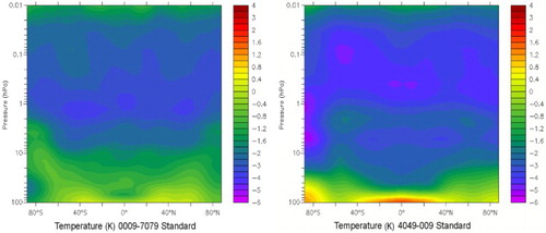
The relatively smaller temperature increases in the polar southern and northern stratosphere are caused by an averaged increasing downwelling in these regions. From 40°S to 40°N at an altitude of about 100 hPa past tropospheric climate change is recognizable in the standard simulation.

b Future Temperature Development in EMAC

1 Simulated stratospheric and mesospheric future climate change

Future increases in GHGs and decreases in ODS lead to a significant cooling in nearly all regions of the stratosphere and mesosphere in the EMAC standard simulation. The general pattern of future temperature development is similar to simulated changes in the past, but the different evolution of ODS leads to some different structures in some regions.

In Figure 1 (right) the future ten-year mean temperature change (2040 to 2049 minus 2000 to 2009) in the standard simulation is shown. The simulated future cooling in the stratosphere and mesosphere is obvious. Here, the strongest cooling with mean temperature differences of −4 to −5 K is simulated above the stratopause and in the Antarctic middle and upper stratosphere. Two relative maxima exist in the region of the middle latitudes and upper stratosphere indicating radiative warming by the ozone recovery (see also Fig. 3). In the lower part of the Antarctic stratosphere warming is simulated, which is mainly caused by ozone recovery (radiative warming, see Section 3b3). In the tropics at an altitude of about 100 hPa future tropospheric climate change is visible.

2 Contribution of increasing greenhouse gases

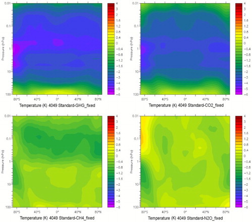
The general cooling in the middle atmosphere is a consequence of the future increase in GHGs (Fig. 2). Here, the increase in CO₂ mixing ratios has the largest influence on this radiative cooling, with mean temperatures decreases in the years 2040 to 2049 of up to −4.5 K in the region of the stratopause. Especially in the stratosphere, CO₂ is almost entirely responsible for the total temperature change caused by GHGs. The cooling rates of CH₄ are small in comparison; hence, the temperature decreases are only about −0.3 to −0.2 K in the stratosphere. In the mesosphere, however, the higher H₂O mixing ratios also have a cooling effect. These higher mesospheric H₂O mixing ratios (see also Fig. 8) are caused by additional oxidation of CH₄ (see Section 4b5). Future H₂O development leads to temperature changes of up to −1.2 K in the mesosphere. The increase in N₂O mixing ratios makes the smallest contribution to stratospheric temperature changes of all the GHGs (about −0.2 K in the tropics and up to −0.6 K in the Arctic). This cooling is an effect of ozone destruction by NO_x (see Section 4b4).

Fig. 2 Contribution of GHGs to the simulated temperature cooling averaged over the years 2040 to 2049. The contribution of GHGs (top left panel; Standard-GHG_fixed), CO₂ (top right panel; Standard-CO₂_fixed), CH₄ (bottom left panel; Standard-CH₄_fixed), and N₂O (bottom right panel; Standard-N₂O_fixed) are derived by subtracting the ten-year temperature mean from 2040 to 2049 of the corresponding sensitivity simulation from the ten-year temperature mean from 2040 to 2049 of the standard simulation.

3 Contribution of decreasing ODS

The simulated ozone recovery by decreasing ODS mixing ratios leads, in general, to a warming of the middle atmosphere in the years 2040 to 2049 (Fig. 3). The warming is evident in the upper stratosphere, with maximum values over 0.8 K in the tropics and mid-latitudes, where the strongest ozone increase takes place (see also Fig. 4, bottom left panel). In the Antarctic lower stratosphere a positive signal for the temperature is visible according to the ozone recovery, but in the Antarctic middle stratosphere this pattern is not obvious. This polar dipole structure is characteristic of dynamical changes and justified by different heating rates, modifications of the polar vortex evolution, and temperature anomalies through variations in the Brewer-Dobson circulation caused by the simulated ozone change.

Fig. 3 Contribution of ODS to the simulated temperature changes averaged over the years 2040 to 2049. The contribution of ODS is derived by subtracting the ten-year temperature mean from 2040 to 2049 of the simulation with fixed ODS from the corresponding ten-year temperature mean of the standard simulation (Standard-CFC_fixed).

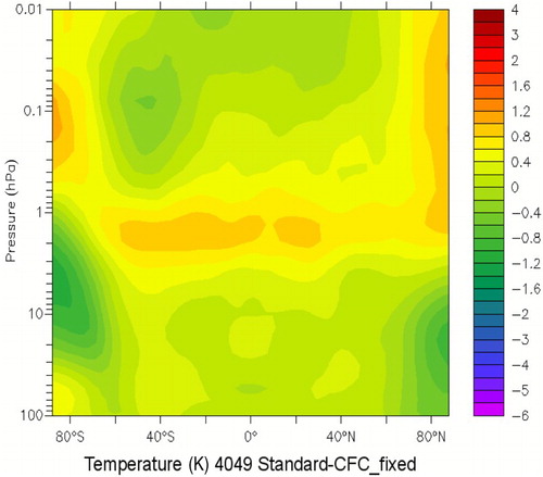
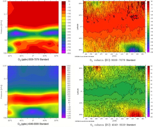
Fig. 4 Simulated ozone depletion and recovery in EMAC. Differences in mean ozone for the years 2000 to 2009 minus the reference period 1970 to 1979 (top panels) and differences for the years 2040 to 2049 minus the reference period 2000 to 2009 (bottom panels) from the standard simulation are illustrated as ozone changes (ppbv) over latitudes and altitudes (left panels) and as time series of ozone columns (Dobson Units) (right panels).

By taking into account the radiative effects of ODS and GHGs, the general pattern of the simulated distribution of future temperature changes in the middle atmosphere in EMAC is understandable (see Fig. 1, right panel). Future climate change in the middle atmosphere is reproduced very well, and model results are in agreement with other model simulations (e.g., Butchart et al., 2010; WMO, 2011). With the help of different sensitivity simulations, determining the contribution from the different GHGs and ODS is also possible. One of the main results of the simulations is that future CO₂ development will have the largest influence on stratospheric and mesospheric climate change. The simulations also show that there is a stronger contribution from CH₄ via H₂O in the mesosphere.

4 Ozone development and contribution of GHGs and ODS to future ozone recovery

a Past Ozone Development in EMAC

The simulated past ozone depletion in EMAC (Fig. 4, top panels) corresponds to the results of different chemistry–climate models performed in previous studies (i.e., Eyring et al., 2006; WMO, 2011). In the EMAC standard simulation the mean ozone change (difference of 2000 to 2009 minus 1970 to 1979) is negative in the entire stratosphere and mesosphere (Fig. 4, top left panel). The highest ozone depletion, with values up to −700 ppbv, is simulated in the upper stratosphere. In the Antarctic lower stratosphere, ozone depletion is dominated by the ozone hole in polar spring. Here negative differences up to −550 ppbv are simulated.

The ozone column averages for 2000 to 2009 (Fig. 4, top right panel) are smaller in all latitudes throughout the entire year, with minor exceptions, than in the years 1970 to 1979. Ozone depletion is especially evident in polar spring in the standard simulation. Here maximum decreases in the ozone column with the highest values up to −120 DU^a are visible during the Antarctic polar spring and during the Arctic polar spring mean differences up to −60 DU are simulated.

b Future Ozone Development in EMAC

1 Simulated ozone recovery

The future ozone recovery simulated by EMAC (Fig. 4, bottom panels) corresponds to projected ozone development in previous studies (i.e., Butchart et al., 2010; WMO, 2011). In nearly all stratospheric regions of the EMAC standard simulation, with the exception of the tropical lower stratosphere, ozone is much higher in the ten-year average for 2040 to 2049 than in the average for 2000 to 2009 (Fig. 4, bottom left panel). In most parts of the mesosphere, however, a decrease in ozone is simulated, with values up to −100 ppbv. The highest positive ozone changes, with values up to 850 ppbv, are obtained in the upper stratosphere and in the Antarctic lower stratosphere (values up to 500 ppbv). The highest negative ozone changes are obtained in the tropical lower stratosphere, with values up to −140 ppbv.

The future ozone columns (Fig. 4, bottom right panel) are higher at almost all latitudes throughout the entire year than the present columns, with the exception of the highest Arctic latitudes from the end of November till the end of December. The ozone recovery in polar spring is particularly evident in our simulations. Here, maximum increases in the ozone column, with mean values up to 80 DU, are visible during the Antarctic polar spring. Also, during the Arctic polar spring, the simulations produce ozone columns that are considerably higher than in the years 2000 to 2009. In the tropics slight ozone increases are simulated.

In the lower tropical stratosphere much lower ozone mixing ratios are simulated in the 2040 to 2049 mean than in the 2000 to 2009 mean (Fig. 4, bottom left) with the result that, despite a strong increase in ozone in the upper stratosphere, the ozone column increases only slightly in the tropics (Fig. 4, bottom right panel). The reason for the lower ozone mixing ratios is an increase in the residual tropical upwelling in EMAC (see Section 4b6).

2 Contribution of decreasing temperatures

The simulated cooler future temperatures in the middle atmosphere caused by increasing CO₂ and CH₄ (Section 3b) lead to an increased ozone buildup (Fig. 5) in almost the entire middle atmosphere. The main reason for this ozone buildup is the temperature dependency of ozone-related chemical reactions, especially within the Chapman Cycle.

Fig. 5 Contribution of GHGs to simulated ozone development averaged over 2040 to 2049. The contribution of GHGs (top left panel; Standard-GHG_fixed), CO₂ (top right panel; Standard-CO₂_fixed), CH₄ (bottom left panel; Standard-CH₄_fixed), and N₂O (bottom right panel; Standard-N₂O_fixed) are derived as in Fig. 2.

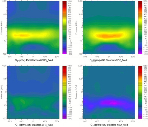
The strongest contributor to ozone production is increasing CO₂ (Fig. 5, top right panel). Here, in the entire middle atmosphere, with the exception of the tropical lower stratosphere, positive ozone changes can be seen. The highest values are simulated in the tropical middle/upper stratosphere with ozone values up to 460 ppbv. In the tropical lower stratosphere ozone decreases in the future. Besides the effect of the enhancing residual vertical upwelling (Section 4b6) a chemical effect due to the change in the overhead ozone column also exists, which affects ultraviolet radiation for the photolysis of oxygen in this region. This chemical effect is simulated (Fig. 5, top right panel) with up to −60 ppbv ozone.

The contribution to ozone development of the increase in CH₄ (Fig. 5, bottom left panel) has two effects. One is the cooling due to additional CH₄ in the lower and middle stratosphere and the additional H₂O formed in the mesosphere, and the other is the chemical effect due to HO_x discussed in Section 4b5. The contribution by cooling is quite visible in the middle/upper stratosphere, but in the mesosphere chemical feedback by HO_x overrides the cooling effect due to H₂O.

3 Contribution of decreasing ODS

Decreasing ODS mixing ratios lead to an ozone recovery that is obvious in almost the entire stratosphere (Fig. 6) with the highest values in the upper stratosphere and in the Antarctic lower stratosphere.

Fig. 6 Contribution of ODS to the simulated ozone development averaged over the years 2040 to 2049 (Standard-CFC_fixed). The contribution of ODS is derived as in Fig. 3.

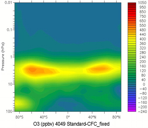
The contribution of decreasing ODS to future ozone increase (Fig. 6) occurs in the middle and upper stratosphere in most regions (with maximum values of ozone up to 480 ppbv in the mid-latitudes in the upper stratosphere) slightly higher than the contribution by GHGs (Fig. 5, top left panel), but it dominates in the Antarctic lower stratosphere. In the tropical lower stratosphere a small decrease in ozone is visible due to the change in photolysis from lower ultraviolet radiation caused by the increase in overhead ozone columns.

4 Contribution of increasing N₂O

In contrast to the influence of decreasing ODS and increasing CO₂, the increase in N₂O mixing ratios leads to intensified ozone destruction (Fig. 5, bottom right panel), caused by higher NO_x mixing ratios (odd nitrogen, comprising NO and NO₂), formed by the reaction of N₂O with atomic oxygen (N₂O + O(¹D) → 2 NO). In Fig. 7 the additional future N₂O is compared with the years 2000 to 2049 and the resulting additional NO_x formed is shown. The mean increase in N₂O from 2040 to 2049 is over 30 ppbv in the troposphere, and the maximum values of resulting additional NO_x formed is over 1 ppbv.

Fig. 7 Distribution of additional N₂O (left) and NO_x (right) averaged over the years 2040 to 2049 due to the future N₂O increase. The additional N₂O and NO_x are derived by subtracting the ten-year mean from 2040 to 2049 of the simulation with fixed N₂O from the corresponding ten-year mean of the standard simulation (Standard-N₂O_fixed).

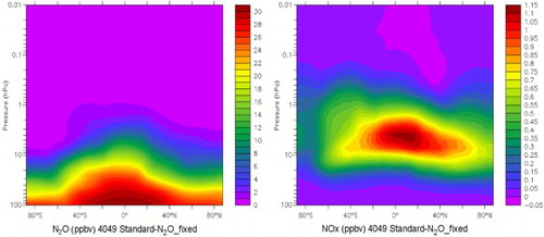
The influence of this additional NO_x on ozone is mainly visible in the middle and upper stratosphere at all latitudes (Fig. 5, bottom right panel). The maximum ozone destruction due to NO_x radicals is up to 220 ppbv in the tropical middle/upper stratosphere; hence, in this region it balances the amount of ozone recovery by decreasing ODS. Relatively high values (up to 120 ppbv) also occur in the Arctic middle stratosphere. In this region, the contribution of NO_x to future ozone development can be very relevant, resulting in a delay in ozone recovery.

5 Contribution of increasing CH₄

Increasing CH₄ mixing ratios result in additional H₂O and HO_x by methane oxidation (CH₄ + OH → CH₃ + H₂O) in the middle atmosphere. Furthermore HO_x is formed mainly in the mesosphere by the following reactions (e.g., le Texier, Solomon, & Garcia, 1988):(1) (2) (3) In summary, increasing CH₄ in the future leads to higher H₂O mixing ratios and additional HO_x, as illustrated in Fig. 8. Additional H₂O is formed in almost the entire middle atmosphere.

Fig. 8 Distribution of additional H₂O (left panel) and HO_x (right panel) averaged over the years 2040 to 2049 due to a future CH₄ increase. The additional H₂O and HO_x are derived by subtracting the ten-year mean from 2040 to 2049 of the simulation with fixed N₂O from the corresponding ten-year mean of the standard simulation (Standard-CH₂_fixed).

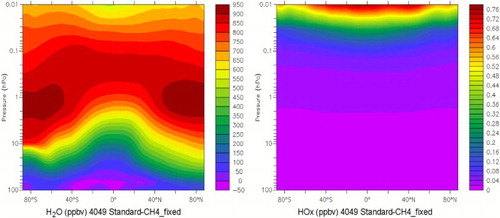
The highest values, with maxima over 900 ppbv, are simulated in the stratopause at high latitudes. HO_x is mainly present in the mesosphere; the higher the altitude the greater the amount of HO_x that is simulated.

The impact of additional HO_x from the increase in CH₄ is additional ozone destruction in the mesosphere. The impact of additional H₂O is radiative cooling in the upper stratosphere and mesosphere, as discussed in Section 3b, connected with the buildup of ozone as discussed in Section 4b2. The combined effect is a decrease in mesospheric ozone as illustrated in Fig. 5 (bottom left panel) caused by the CH₄ increase, with the lowest value being −40 ppbv.

6 Dynamical impact on ozone change

In the EMAC simulations, the enhancement of the Brewer-Dobson circulation plays an important role in future ozone development in different regions. To evaluate this dynamical influence (Fig. 9) the difference between the future ozone change in the standard simulation (Fig. 4, bottom left panel) and the total chemical contribution to future ozone development (i.e., the contribution of CO₂, CH₄, N₂O, and ODS (Figs 5 and 6)) is calculated.

Fig. 9 Dynamical impact on simulated ozone development averaged over the years 2040 to 2049. The dynamical impact is calculated by subtracting the sum of the contributions of CO₂, CH₄, N₂O, and CFCs to the mean ozone change from 2040 to 2049 from the total ozone change from 2040 to 2049 minus 2000 to 2009 of the standard simulation.

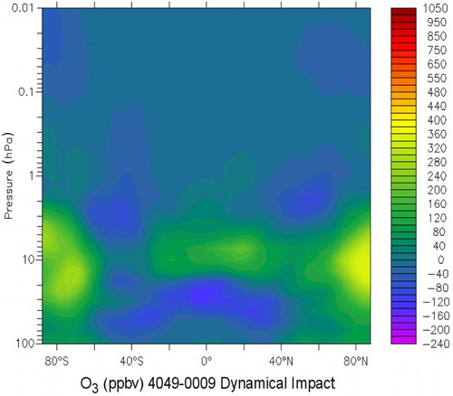
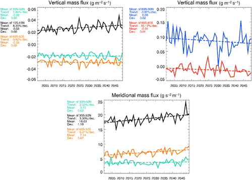
In the tropical lower stratosphere, accelerating residual vertical and meridional wind velocities lead to less ozone in the future. In the EMAC simulation, decreasing ozone mixing ratios caused by a change in transport are simulated from 2040 to 2049 between 50°S and 40°N and 20 and 80 hPa (Fig. 9). Lower ozone mixing ratios with differences up to −120 ppbv exist in the lower tropical stratosphere as a result of higher vertical and meridional mass fluxes. This is considerably more than the chemical effect due to the increased overhead ozone columns mentioned in Section 4b2. Hence, in the EMAC simulation the changed mass fluxes will dominate future ozone in this region. In Fig. 10 the mass fluxes at 54 hPa calculated from the residual vertical velocity and the meridional velocities of the standard simulation are illustrated from 2000 to 2050. The strongest vertical mass fluxes in the EMAC simulation exist in the tropical regions (Fig. 10, top left panel) with annual means between 0.02 and 0.04 g m⁻² s⁻¹ and a positive trend of 1.8% per decade. A downward transport exists in the average for the mid-latitudes with values between −0.01 and −0.04 g m⁻² s⁻¹. The average downward transport increases from 2000 to 2050 with a trend of 1.8% per decade and 0.92% per decade in the northern and southern mid-latitudes, respectively. The yearly average poleward meridional mass fluxes (Fig. 10, bottom panel) are positive in all latitudes between 60°S and 60°N at 54 hPa with the highest mass fluxes being between 15 and 25 g m⁻² s⁻¹ and a positive trend of 3.3% per decade from 30°S to 30°N. In the mid-latitudes, the meridional mass fluxes are lower but still positive and also have positive trends. Considering the residual vertical and meridional mass fluxes and their trends the simulated lower future ozone mixing ratios (Fig. 9) can be explained by accelerated upward and poleward transport.

Fig. 10 Annual means of vertical residual (top panel) and meridional (bottom panel) mass fluxes at 54 hPa (approximately 20.5 km) from the standard simulation. Poleward meridional mass flux is positive.

In the tropical upper stratosphere closer to 10 hPa the residual vertical velocity has a minimum in the standard EMAC simulation and also partly turns around and even increases in the future (not shown). Because meridional transport plays a much smaller role, as in lower regions, an average increase in ozone as a result of the residual vertical transport with additional ozone mixing ratios up to 160 ppbv is simulated (Fig. 9).

In the southern and northern polar regions the residual vertical velocities have a future downward forcing (Fig. 10, top right panel). So in northern polar latitudes at 54 hPa the vertical mass flux is, on average, positive with values between 0.05 and 0.15 g m⁻² s⁻¹ and a mean of 0.09 g m⁻² s⁻¹, but has a negative trend of −3.97% per decade. In southern polar latitudes the annual average residual vertical mass fluxes are mostly negative with values between −0.05 and 0.02 g m⁻² s⁻¹ with a mean of −0.01 g m⁻² s⁻¹. This downward transport accelerates in the future. As a result of this polar downward forcing, which is also simulated below and above 54 hPa (not shown), increasing ozone mixing ratios are simulated between 2 hPa and 100 hPa in the southern and northern polar regions (Fig. 9). Additional O₃ mixing ratios occur in northern polar regions with maxima up to 340 ppbv, which is slightly higher than the values in the southern polar region with maxima up to 260 ppbv.

In summary, the enhancement of the Brewer-Dobson circulation in the EMAC simulations has a large impact on future ozone distribution in the lower and middle stratosphere. In polar regions, especially in northern high latitudes, at some altitudes the dynamical impact on future ozone (Fig. 9) is more positive than the ozone increase due to GHGs, especially in northern polar regions (Fig. 5, top left panel). In the tropical lower stratosphere the contribution from increased residual vertical upwelling leads to decreasing ozone due to the vertical transport of ozone-poor air from below. This effect is much higher than the impact of chemical change due to the increased overhead ozone columns (Fig. 5, top right panel and Fig. 6).

7 Global averaged ozone recovery and contribution by increasing Ghgs and Decreasing ODS

In Fig. 11 the global average ozone change and the contributions due to ODS, GHGs, CO₂, CH₄, and N₂O are illustrated. The results discussed so far can also be seen in this graph.

Fig. 11 Simulated ozone change in EMAC simulations. Differences in global ten-year ozone means for the years 2040 to 2049 minus the reference period 2000 to 2009 (total in red) and the contribution from ODS (green), GHGs (blue), CO₂ (light blue), CH₄ (purple), and N₂O (black).

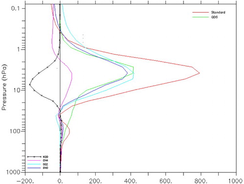
Hence, ozone recovery in the middle and upper stratosphere (maximum values of ozone from nearly 800 ppbv) is primarily driven by the future decrease in ODS (maximum values greater than 400 ppbv) and by the future increase in GHGs (maximum values of about 380 ppbv) with a positive contribution nearly as high as the contribution from ODS. The contribution due to CO₂ alone (maximum values greater than 400 ppbv) is even higher than the contribution from ODS, especially in the middle stratosphere. In the lower stratosphere, the CO₂ contribution dominates the contribution from ODS.

The contribution to ozone recovery from increasing N₂O is negative in the middle stratosphere (reducing the values by up to 180 ppbv). At altitudes between 10 and 20 hPa global average ozone destruction due to the additional NO_x (formed by increasing N₂O) is equal to the global average ozone recovery from decreasing ODS.

In most of the mesosphere (above 0.4 hPa) the global average ozone change is negative. The additional HO_x formed by the future CH₄ increase is responsible for this ozone decrease.

5 Conclusions

With the help of a standard simulation and different sensitivity simulations, it was possible to assess the different contributions of GHGs and ODS to the future development of temperature and ozone according the IPCC A1B scenario and the WMO Ab scenario.

Stratospheric and mesospheric climate change is influenced by different factors, but with the performed EMAC simulations, we can determine that the future increase in CO₂ will have the largest influence on temperature change, followed by the future increase in CH₄ (radiative cooling by CH₄ in the stratosphere and additional cooling by increasing H₂O in the upper stratosphere and mesosphere). The future increase in N₂O makes a small contribution to the cooling. Future ozone recovery will lead to a warming of the middle atmosphere, but heating due to increasing ozone is much lower than the cooling due to increasing CO₂.

Future ozone recovery is primarily driven by the future decrease in ODS but also by the increase in ozone from radiative cooling due to the GHGs in the middle atmosphere.

In the middle and upper stratosphere the total effect of GHGs on the future increase in ozone in most regions is almost as high as the contribution from the decrease in ODS. But in the Antarctic lower stratosphere, the impact of ODS is dominant. The strongest contribution to the increase in ozone due to radiative cooling is not only caused by increasing CO₂ mixing ratios but also by increasing CH₄ mixing ratios although with lower amounts (especially in the mesosphere also via the formation of H₂O).

Besides the impact due to climate change there are also chemical feedbacks caused by GHGs. Here, the future increase in CH₄ leads to the formation of additional HO_x, resulting in a decrease in mesospheric ozone. The future increase in N₂O also has a chemical effect, resulting in a delay in ozone recovery in the middle and upper stratosphere from additional ozone-depleting catalytic cycles with NO_x. In the middle stratosphere in particular the amount of ozone destruction by NO_x in some regions is of similar importance to the amount of the increase in ozone from decreasing ODS.

In the stratosphere the enhancement of the Brewer-Dobson circulation has a strong impact on future ozone distribution. In polar regions, increased downwelling leads to additional ozone in the entire stratosphere. In polar regions, especially at northern high latitudes, the dynamical impact on ozone development is, at some altitudes, higher than the increase in ozone due to cooler future temperatures caused by increased GHGs. In the tropical lower stratosphere the contribution from increased residual vertical upwelling dominates the future decrease in ozone.

With the help of our study it is possible to complement published scientific results of, for example, Eyring et al. (2010a, 2010b), Fleming et al. (2011), Oman et al. (2010), and Revell et al. (2012) regarding the contributions of CO₂, CH₄, N₂O, GHGs to and the influence of the Brewer-Dobson circulation on future stratospheric and mesospheric climate change and ozone recovery.

The major factors for the recovery of ozone in the future are decreasing ODS, cooling in the middle atmosphere caused mainly by the increase in CO₂ and also changes in the Brewer-Dobson circulation. In the upper stratosphere the total effect of GHGs on the future increase in ozone is nearly as high as the contribution from the decrease in ODS. The chemical effects of the additional NO_x and HO_x formed due to the increase in CH₄ and N₂O are not negligible and in some regions are of essential importance, especially in the middle stratosphere (NO_x) and in the mesosphere (HO_x). The changed transport due to an enhanced Brewer-Dobson circulation has a crucial impact on the polar stratosphere and also on the tropical lower stratosphere.

Notes

^aDU = 0.01 mm at standard temperature and pressure and is equivalent to 2.69 × 10²⁰ molecules per square metre

References

- Barnett, J. J., Houghton, J. T., & Pyle, J. A. (1975). The temperature dependence of the ozone concentration near the stratopause. Quarterly Journal of the Royal Meteorological Society, 101, 245–257. doi:10.1002/qj.49710142808
- Butchart, N., Cionni, I., Eyring, V., Shepherd, T. G., Waugh, D. W., Akiyoshi, H., … Tian, W. (2010). Chemistry–climate model simulations of twenty-first century stratospheric climate and circulation changes. Journal of Climate, 23, 5349–5374. doi:10.1175/2010JCLI3404.1
- Butchart, N., Scaife, A. A., Bourqui, M., de Grandpré, J., Hare, S. H. E., Kettleborough, J., … Sigmond, M. (2006). Simulations of anthropogenic change in the strength of the Brewer–Dobson circulation. Climate Dynamics, 27, 727–741. doi:10.1007/s00382-006-0162-4
- Chapman, S. (1930). On ozone and atomic oxygen in the upper atmosphere. Philosophical Magazine, 10, 369. doi:10.1080/14786443009461588
- Chipperfield, M. P., & Feng, W. (2003). Comment on: “Stratospheric ozone depletion at northern mid-latitudes in the 21st century: The importance of future concentrations of greenhouse gases nitrous oxide and methane.” Geophysical Research Letters, 30(7), 1389. doi:10.1029/2002GL016353
- Eyring, V., Butchart, N., Waugh, D. W., Akiyoshi, H., Austin, J., Bekki, S., … Yoshiki, M. (2006). Assessment of temperature, trace species, and ozone in chemistry-climate model simulations of the recent past. Journal of Geophysical Research, 111, D22308. doi:10.1029/2006JD007327
- Eyring, V., Cionni, I., Bodeker, G. E., Charlton-Perez, A. J., Kinnison, D. E., Scinocca, J. F., … Yamashita, Y. (2010a). Multi-model assessment of stratospheric ozone return dates and ozone recovery in CCMVal-2 models. Atmospheric Chemistry and Physics, 10, 9451–9472. doi:10.5194/acp-10-9451-2010
- Eyring, V., Cionni, I., Lamarque, J. F., Akiyoshi, H., Bodeker, G. E., Charlton-Perez, A. J., … Yamashita, Y. (2010b). Sensitivity of 21st century stratospheric ozone to greenhouse gas scenarios. Geophysical Research Letters, 37, L16807. doi:10.1029/2010GL044443
- Eyring, V., Waugh, D. W., Bodeker, G. E., Cordero, E., Akiyoshi, H., Austin, J., … Yoshiki, M. (2007). Multimodel projections of stratospheric ozone in the 21st century. Journal of Geophysical Research, 112, D16303. doi:10.1029/2006JD008332
- Fleming, E. L., Jackman, C. H., Stolarski, R. S., & Douglass, A. R. (2011). A model study of the impact of source gas changes on the stratosphere for 1850–2100. Atmospheric Chemistry and Physics, 11, 8515–8541. doi:10.5194/acp-11-8515-2011
- Garcia, R. R., & Randel, W. J. (2008). Acceleration of the Brewer–Dobson circulation due to increases in greenhouse gases. Journal of the Atmospheric Sciences, 65, 2731–2739. doi:10.1175/2008JAS2712.1
- Haigh, J. D., & Pyle, J. A. (1979). A two-dimensional calculation including atmospheric carbon dioxide and stratospheric ozone. Nature, 279, 222–224. doi:10.1038/279222a0
- Intergovernmental Panel on Climate Change. (2007). Climate Change 2007: Synthesis Report. A Contribution of Working Groups I, II and III to the Fourth Assessment Report of the Intergovernmental Panel on Climate Change [Core Writing Team, Pachauri, R. K., & Reisinger, A.]. Geneva, Switzerland: IPCC.
- Jöckel, P., Sander, R., Kerkweg, A., Tost, H., & Lelieveld, J. (2005). Technical Note: The Modular Earth Submodel System (MESSy) – a new approach towards Earth System Modeling. Atmospheric Chemistry and Physics, 5, 433–444. doi:10.5194/acp-5-433-2005
- Jöckel, P., Tost, H., Pozzer, A., Brühl, C., Buchholz, J., Ganzeveld, L., … Lelieveld, J. (2006). The atmospheric chemistry general circulation model ECHAM5/MESSy1: Consistent simulation of ozone from the surface to the mesosphere. Atmospheric Chemistry and Physics, 6, 5067–5104. doi:10.5194/acp-6-5067-2006
- Kirner, O., Ruhnke, R., Buchholz-Dietsch, J., Jöckel, P., Brühl, C., & Steil, B. (2011). Simulation of polar stratospheric clouds in the chemistry-climate-model EMAC via the submodel PSC. Geoscientific Model Development, 4, 169–182. doi:10.5194/gmd-4-169-2011
- Kohlhepp, R., Ruhnke, R., Chipperfield, M. P., De Mazière, M., Notholt, J., Barthlott, S., … Wood, S. W. (2012). Observed and simulated time evolution of HCl, ClONO2, and HF total column abundances. Atmospheric Chemistry and Physics, 12, 3527–3556. doi:10.5194/acp-12-3527-2012
- le Texier, H., Solomon, S., & Garcia, R. R. (1988). The role of molecular hydrogen and methane oxidation in the water vapour budget of the stratosphere. Quarterly Journal of the Royal Meteorological Society, 114, 281–295. doi:10.1002/qj.49711448002
- Oman, L. D., Plummer, D. A., Waugh, D. W., Austin, J., Scinocca, J. F., Douglass, A. R., … Ziemke, J. R. (2010). Multimodel assessment of the factors driving stratospheric ozone evolution over the 21st century. Journal of Geophysical Research, 115, D24306. doi:10.1029/2010JD014362
- Portmann, R. W., & Solomon, S. (2007). Indirect radiative forcing of the ozone layer during the 21st century. Geophysical Research Letters, 34, L02813. doi:10.1029/2006GL028252
- Randeniya, L. K., Vohralik, P. F., & Plumb, I. C. (2002). Stratospheric ozone depletion at northern mid latitudes in the 21st century: The importance of future concentrations of greenhouse gases nitrous oxide and methane. Geophysical Research Letters, 29(4), 1051. doi:10.1029/2001GL014295
- Revell, L. E., Bodeker, G. E., Huck, P. E., Williamson, B. E., & Rozanov, E. (2012). The sensitivity of stratospheric ozone changes through the 21st century to N2O and CH4. Atmospheric Chemistry and Physics, 12, 11309–11317. doi:10.5194/acp-12-11309-2012
- Roeckner, E., Brokopf, R., Esch, M., Giorgetta, M., Hagemann, S., Kornblueh, L., … Schulzweida, U. (2006). Sensitivity of simulated climate to horizontal and vertical resolution in the ECHAM5 atmosphere model. Journal of Climate, 19, 3771–3791. doi:10.1175/JCLI3824.1
- Rosenfield, J. E., Douglass, A. R., & Considine, D. B. (2002). The impact of increasing carbon dioxide on ozone recovery. Journal of Geophysical Research, 107(D6), 4049. doi:10.1029/2001JD000824
- Sander, R., Kerkweg, A., Jöckel, P., & Lelieveld, J. (2005). Technical note: The new comprehensive atmospheric chemistry module MECCA. Atmospheric Chemistry and Physics, 5, 445–450. doi:10.5194/acp-5-445-2005
- Sander, S. P., Abbatt, J., Barker, J. R., Burkholder, J. B., Friedl, R. R., Golden, D. M., … Wine, P. H. (2011). Chemical kinetics and photochemical data for use in atmospheric studies (Evaluation No. 17. JPL Publication 10-6). Pasadena: Jet Propulsion Laboratory.
- Sander, S. P., Friedl, R. R., Ravishankara, A. R., Golden, D. M., Kolb, C. E., Kurylo, M. J., … Finlayson-Pitts, B. J. (2003). Chemical kinetics and photochemical data for use in atmospheric studies (Evaluation Number 14. JPL Publication 02-25). Pasadena: Jet Propulsion Laboratory.
- SPARC CCMVal. (2010). Report on the Evaluation of Chemistry-Climate Models (SPARC Report No. 5, WCRP-132, WMO/TDNo. 1526) [V. Eyring, T. G. Shepherd, & D. W. Waugh]. Retrieved from http://www.sparc-climate.org
- World Meteorological Organization. (2007). Scientific Assessment of Ozone Depletion: 2006 (Global Ozone Research and Monitoring Project-Report No. 50). Geneva, Switzerland: World Meteorological Organization.
- World Meteorological Organization. (2011). Scientific Assessment of Ozone Depletion: 2010 (Global Ozone Research and Monitoring Project-Report No. 52). Geneva, Switzerland: World Meteorological Organization.