Impacts of Climate Change in the Gulf of St. Lawrence

ABSTRACT

To explore modifications in water temperature and salinity under warmer climate change conditions, we performed simulations from 1970 to 2069 with the CANadian Océan PArallélisé (CANOPA) model for the Gulf of St. Lawrence and the Scotian Shelf. The surface fields to drive CANOPA were provided by the Canadian Regional Climate Model (CRCM), driven by the outputs from the third-generation Canadian Global Climate Model (CGCM3) following the Intergovernmental Panel on Climate Change (IPCC) Special Report on Emissions Scenarios (SRES) A1B climate change scenario. The sea-ice concentration and volume simulated by CANOPA are shown to have patterns consistent with those seen in observations; CANOPA is also shown to simulate sea surface temperature (SST) well. Although CANOPA can simulate the observed vertical structure of water temperature and salinity, it tends to underestimate the cold intermediate layer and overestimate water salinity in the central Gulf of St. Lawrence (GSL). In terms of the possible future climate, CANOPA simulations suggest that the GSL will be largely ice free in January, with ice volume in March steadily decreasing from about 80 km³ in the 1980s to near zero by the late 2060s. On average, the GSL water will become warmer and fresher over this time period. In January, maximum SST increases occur near eastern Cabot Strait, with amplitudes of about 1.5°–2.5°C, corresponding to reduced sea ice in that area, and there is no notable change along the western and northern coasts of the GSL. In July, maximum SST increases occur over the western GSL corresponding to the largest increases in surface air temperature in the region. The maximum decreases in surface salinity also occur near western coastal areas and the Scotian Shelf, whereas reductions in the eastern GSL are relatively weak. Finally, compared with the present climate, the cold intermediate layer is significantly weaker in 2040–2069 than in 1980–2009.

RÉSUMÉ

[Traduit par la rédaction] Afin d'explorer les modifications dans la température et la salinité de l'eau sous l'effet d'un réchauffement climatique, nous avons effectué des simulations pour la période allant de 1970 à 2069 avec le modèle CANadian Océan PArallélisé (CANOPA) pour le golfe du Saint-Laurent et la plate-forme Néo-Écossaise. Les champs de surface utilisés pour piloter le CANOPA provenaient du Modèle régional canadien du climat (MRCC), lui-même piloté par les sorties du modèle canadien du climat mondial de troisième génération (CGCM3) selon le scénario de changement climatique A1B du Rapport spécial sur les scénarios d’émissions (SRES) du Groupe d'experts intergouvernemental sur l’évolution du climat (GIEC). Il apparaît que la concentration et de volume de glaces de mer simulés par le CANOPA ont des configurations qui s'accordent avec celles que l'on trouve dans les observations; le CANOPA simule bien, également, la température de surface de la mer (TSM). Bien que le CANOPA puisse simuler la structure verticale observée de la température et de la salinité de l'eau, il a tendance à sous-estimer la couche intermédiaire froide et à surestimer la salinité de l'eau dans le golfe du Saint-Laurent. En ce qui a trait au climat futur possible, les simulations du CANOPA suggèrent que le golfe sera principalement libre de glace en janvier, avec un volume de glace en mars diminuant régulièrement d'environ 80 km³ dans les années 1980 jusqu’à près de zéro vers la fin des années 2060. En moyenne, l'eau du golfe deviendra plus chaude et plus douce au cours de cette période. En janvier, les accroissements maximums de la TSM se produisent près du côté est du détroit de Cabot, avec des amplitudes d'environ 1,5 à 2,5 °C, ce qui concorde avec la réduction de la glace de mer dans cette région, et il n'y a pas de changement notable le long des côtes ouest et nord du golfe. En juillet, les accroissements maximums de la TSM se produisent dans l'ouest du golfe, ce qui concorde avec les plus fortes augmentations de la température de l'air en surface dans la région. Les réductions maximales de la salinité en surface se produisent aussi près des régions côtières ouest et de la plate-forme Néo-Écossaise, alors que les réductions dans l'est du golfe sont relativement faibles. Finalement, comparativement au climat actuel, la couche intermédiaire froide est nettement plus faible durant la période 2040–2069 que durant la période 1980–2009.

KEYWORDS:

• climate change
• Gulf of St. Lawrence
• 2040–2069
• decreased sea ice
• warming temperatures
• cold intermediate layer
• decreased surface salinity

1 Introduction

The Gulf of St. Lawrence (GSL) is almost an inland sea opening to the Atlantic Ocean through Cabot Strait and the Strait of Belle Isle. It receives large quantities of fresh water from the St. Lawrence River. The inflow through the Strait of Belle Isle and Cabot Strait circulates cyclonically in the GSL before exiting through Cabot Strait (Han, Loder, & Smith, 1999). Because the GSL is the habitat of many fishery stocks, at various stages of life, it is important to understand the possible changes that may occur in water temperature and salinity in a warmer climate.

The GSL vertical water temperature structure varies from a two-layer system in winter to a three-layer system in summer (Galbraith, 2006). In winter, the GSL is partially covered by sea ice, and the surface temperature is near freezing, but the deep layer is a relatively warm mixture of Labrador and Slope Water. In the spring, a warm surface layer develops as a result of increased surface heat flux. Below the warm surface water is a cold intermediate layer (CIL), the remnant from the previous winter, which is characterized by a temperature minimum below −1°C. Total CIL volume varies interannually from 10,000 to 15,000 km³; the dominant processes are interannual variations in the in situ cold water formation, the inflow of cold saline water from the Labrador Shelf, and the inflow of warmer water along the eastern side of Cabot Strait (Galbraith, 2006).

To understand the physical processes associated with water mass formation in the GSL, coastal ocean models have been employed in several studies (Han et al., 1999; Saucier, Roy, Gilbert, Perrin, & Ritchie, 2003; Smith, Saucier, & Staub, 2006). In contrast to general circulation models (GCMs), coastal ocean models allow for long-term simulations with a high horizontal resolution at a relatively low computational cost. Although a coastal ocean model can reasonably simulate the formation and circulation of water mass and sea ice in the region, the accuracy of the atmospheric surface driving fields is critical to the accuracy of the resulting simulated ocean circulation (Saucier et al., 2003). In climate change studies, GCMs typically have a horizontal resolution of approximately 200–300 km (McFarlane, Boer, Blanchet, & Lazare, 1992), which is too coarse to provide good estimates for the GSL.

The objective of this paper is to investigate the impacts of climate change on the mean state of the waters and sea ice in the GSL. Section 2 describes the models and the experimental design. Section 3 shows the current climatology, demonstrating that our model can reliably reproduce the present climatology. The impacts of climate change are given in Section 4, and Section 5 presents the conclusions.

2 Model description and experiment design

a Atmospheric Model

The Canadian Regional Climate Model (CRCM) is based on the dynamical formulation of the Canadian Mesoscale Compressible Community (MC2) model and solves the fully elastic nonhydrostatic Euler equations using a semi-implicit semi-Lagrangian numerical scheme (Caya & Laprise, 1999). The physical parameterization package of the second-generation Canadian Global Climate Model (CGCM2), following McFarlane et al. (1992), is implemented to solve the subgrid-scale processes. The Kain–Fritsch scheme is used for deep convection, and large-scale condensation is simulated using the CGCM2 physics formulation (Kain & Fritsch, 1990; Paquin & Caya, 2001). In this study, the CRCM was implemented over a domain focused on eastern Canada and the northeastern Atlantic (Fig. 1a). The simulations were performed at a horizontal resolution of 25 km, with 29 levels in the vertical direction. A 15-minute time step was employed. A detailed description of CRCM is given by Caya and Laprise (1999), Laprise, Caya, Frigon, and Paquin (2003), and Caya and Biner (2004).

Fig. 1 Model domains for (a) the CRCM and (b) NEMO. Two comparison locations are indicated at “A” (60.9833°W, 47.0333°N) and “B” (60.6333°W, 48.48333°N), which are used in Figs 7 and 8. SBI: Strait of Belle Isle, GSL: Gulf of St. Lawrence, SLE: St. Lawrence estuary.

b Ocean Model

The CAnadian OPA (CANOPA) model was developed at the Bedford Institute of Oceanography (Brickman & Drozdowski, 2012), based on the Océan PArallélisé, version 9 (OPA 9.0; Madec, Delecluse, Imbard, & Lévy, 1998) model and the Louvain-la-Neuve ice model, version 2 (LIM2; Fichefet & Morales Maqueda, 1997; Bouillon, Morales Maqueda, Legat, & Fichefet, 2009). The temperature and salinity were created from data available from the Department of Fisheries and Oceans (DFO) hydrographic climate database, interpolated onto the CANOPA grid, using an optimal interpolation technique. Forced with water temperature and salinity from the DFO observational database and Coordinated Ocean-ice Reference Experiments (CORE) atmospheric surface fields (Large & Yeager, 2008), CANOPA provides reasonable simulations of ocean transport along the Scotian Shelf compared with observations (Brickman & Drozdowski, 2012). Although the simulated total ice volume is within the error bars of the observations, CANOPA tends to underestimate ice volume during the melt season. Moreover, in this study, CANOPA was further tuned using the surface forcing from the CRCM-downscaled atmospheric fields and lateral boundary conditions, based on adjusted simulations from the third-generation Canadian Global Climate Model (CGCM3). Additional details on CANOPA can be found in Brickman and Drozdowski (2012).

The OPA model is a three-dimensional, hydrostatic, primitive equation model with complete thermohaline dynamics. Horizontal diffusion and viscosity are handled by a Laplacian scheme with its coefficients computed by a Smagorinsky scheme. A widely used Mellor–Yamada turbulence kinetic energy (TKE) scheme is employed to represent the vertical mixing dynamics (Mellor & Yamada, 1982), denoted MY2.5. The CANOPA model is tuned to the TKE scheme to make sure it has a reasonable representation of observed features. Moreover, the M₂ tide was implemented in the CANOPA model. Vertical convection is accomplished using an enhanced vertical diffusion scheme with the diffusivity coefficient set to 5 m² s⁻¹ when the water column is unstable. Bathymetry for the model is derived from a combination of Atlantic Geoscience Centre (AGC) measurement data, Earth Topography 2-arc-min (ETOPO2) data, and the archived measurement data from the DFO Gulf Region. The grid was selected as a subset of the Nucleus for European Modelling of the Ocean (NEMO) tri-polar global spherical coordinate domain, for which OPA is its ocean component. The horizontal resolution is 1/12° with 46 vertical z-levels (the first 10 w-levels are approximately at 0, 6, 13, 20, 28, 37, 47, 58, 71, and 85 m). The time step is 480 s. The model domain covers the GSL, the Scotian Shelf, and the Gulf of Maine (Fig. 1b).

The sea-ice component is LIM2. It is a two-level thermodynamic–dynamic sea-ice model. Sensible heat storage and vertical heat conduction within snow and ice are determined by a three-layer model (one layer for snow and two layers for ice). The effect of the subgrid-scale snow and ice thickness distributions is implicitly accounted for through an effective thermal conductivity. The storage of latent heat inside the ice, resulting from the trapping of shortwave radiation by brine pockets, is taken into account. Vertical and lateral growth and decay rates of the ice are obtained from prognostic energy budgets at both the bottom and surface boundaries of the snow–ice cover and in leads. The surface albedo depends on the state of the surface, the snow and ice thicknesses, and the cloudiness. When the snow load is sufficiently large to depress the snow–ice interface under the open ocean water level, it is suggested that sea water infiltrates the entirety of the submerged snow and freezes there, forming ice. Ice dynamics are simulated by assuming that sea ice behaves as a two-dimensional viscous–plastic continuum in dynamical interaction with the atmosphere and ocean. The ice momentum and transport equations are written in curvilinear, orthogonal coordinates and are numerically solved on a B-grid. For the transport equation, a numerical method that conserves the second-order moments of the spatial distribution of the advected quantity is used (Bouillon et al., 2009; Fichefet & Morales Maqueda, 1997). Ice–water and air–ice drag coefficients are set to 5.5 × 10⁻³ and 2.3 × 10⁻³, respectively.

c Experiment Design

Large-scale circulation can be reasonably simulated by CGCM3 compared with other GCMs that participated in the Intergovernmental Panel on Climate Change (IPCC) fourth assessment report (AR4; Randall et al., 2007). However, output from the atmospheric component of the CGCM3 has a horizontal resolution of about 2.5°, and the resolution of the ocean component of CGCM3 is about 1.85°; these are too coarse to simulate the detailed features of the sea-ice edge, the marginal ice zone, or the detailed fine-resolution ocean circulation. Therefore, CRCM is used to downscale CGCM3 simulations to provide high-resolution surface fields to drive CANOPA.

The CGCM3 simulations tend to overestimate sea surface temperature (SST) in the GSL, which leads to significant bias in surface wind speeds in CRCM simulations (Guo et al., 2013). To reduce the bias, the CGCM3 SST fields were corrected using the North American Regional Reanalysis (NARR; Mesinger et al., 2006) six-hourly SST climatology following Guo et al. (2013). Specifically, the following relation was applied:(1)

where and are six-hourly SST averages from CGCM3 simulations and NARR data for the 1979–2008 period. The NARR has a horizontal resolution of 32 km and includes assimilation of precipitation along with other variables. This approach effectively removes the bias in the CGCM3 SST present climatology but keeps the CGCM3 SST variability and long-term trends. In the CRCM simulations, sea ice is specified by the CGCM3 outputs. Thus, if the grid is covered with sea ice, CRCM uses the ice surface temperature, as estimated using the energy balance equation.

For CANOPA temperature and salinity, the lateral boundary conditions are specified by the CGCM3 simulation. To minimize model drift, the CGCM3 long-term mean (1979–2008) was replaced with estimates of temperature and salinity suggested by Levitus (1982), but the variability and long-term trend in the CGCM3 simulation were kept. This is similar to the correction for SST in Eq. (1). The correction is applied to the entire dataset from 1970 to 2069. It should be noted that Levitus data represent the 1900–1997 climatology, whereas the CGCM3 long-term mean is computed using the 1979–2008 data. Moreover, it appears that slight shifts in the Levitus data do not have significant effects because the climatology simulated by CANOPA is comparable to Levitus data. Because the GSL is relatively shallow, the changes in water temperature and salinity are mainly associated with river runoff and surface forcing, and the effects of the temporal discrepancy are relatively small. Based on observations, an annual cycle of the barotropic transport is prescribed at both Cabot Strait and at the Strait of Belle Isle, superimposed on the baroclinic transport as calculated from the adjusted CGCM3 water temperature and salinity fields. We should also mention that, because of the coarse resolution of CGCM3, the water temperature and salinity at neighbouring points are used to estimate the baroclinic transport for the Strait of Belle Isle.

A simple hydrology model was developed to estimate river runoff from the CRCM simulation to constrain CANOPA (Lambert et al., 2013). In this methodology, the watershed information was extracted from the Global River Network USGS Hydrological data and maps based on the SHuttle Elevation Derivatives at multiple Scales (HydroSHEDS) dataset (http://hydrosheds.cr.usgs.gov/index.php). The hydrology model was calibrated and validated using station data, forced with data from the National Centers for Environment Prediction (NCEP; Kalnay et al., 1996). Thus, the freshwater volume was estimated using the rates of precipitation and evaporation from CRCM-downscaled fields. In addition, the model uses surface air temperature (SAT) to determine if the precipitation occurs as rain or snow. There are 78 rivers in CANOPA for the domain used in this study. Thus, it can be shown that the hydrology model can reproduce the observed magnitude and variability of river runoff in eastern Canada (Fig. 4 in Lambert et al., 2013).

3 Present climatology

a Surface Air Temperature

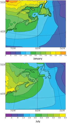
Here, we compare the CRCM simulations with NCEP data to emphasize the advantage of high-resolution CRCM downscaling. Using both NARR and station data, the detailed validations of simulated surface wind and SAT are given by Guo et al. (2013), suggesting that CRCM can reproduce SAT and surface wind well. Compared with the NCEP reanalysis, Fig. 2 shows that CRCM can reproduce the spatial patterns of the large-scale SAT reasonably well. In winter, the spatial variability is dominated by the land–sea contrast associated with the different heat capacities of land and water, and the temperature gradient is distributed along the Canadian coastline, whereas the SAT over land is relatively colder than over the ocean. However, the SAT has stronger meridional gradients in summer than in winter, suggesting the dominant effects of solar radiation. Compared with NCEP reanalyses, CRCM underestimates SAT over the east coast of Newfoundland.

Fig. 2 Surface air temperature (°C) in January (upper panels) and July (lower panels), averaged over the 1970–1999 period.

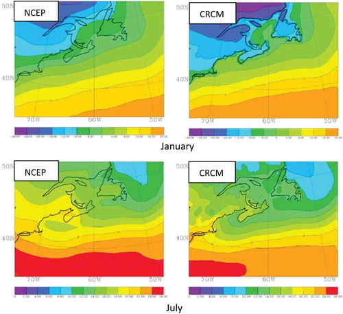
Comparisons between CRCM simulations and NCEP reanalyses also show the advantage of high-resolution CRCM simulations in representing the detailed SAT distribution. Because of its coarse resolution (approximately 1.8°), the GSL is not well represented in the NCEP reanalyses. In January, because of more rapid cooling over land than over water, high-resolution data from the CRCM show that SATs over Nova Scotia, Newfoundland, and several islands in the GSL (such as the Îles-de-la-Madelaine) are colder than over the nearby water. In addition, warm Atlantic water entering the GSL through Cabot Strait increases the SAT in the region (Guo et al., 2013). These characteristics are well captured in the CRCM simulation, whereas results from the NCEP reanalyses show a more uniform spatial pattern. However, in July, when the land–sea contrast is relatively weak, the NCEP reanalysis data and CRCM simulation results are more consistent in the fine-resolution details (Fig. 2).

b Surface Wind

Generally, the surface wind is stronger over water than over land (Fig. 3) because of the smaller drag coefficient of the ocean surface. However, the seasonal variation of surface wind depends on the static stability of the planetary atmospheric boundary layer. Unstable conditions can enhance the energy transport from the upper atmosphere to the surface (Long & Perrie, 2012). In winter, the ocean surface is warmer than the atmosphere, and the stability over the ocean is relatively weak. But the ocean surface is cold in summer, and the atmospheric boundary layer is relatively stable. Therefore, surface winds along the coast of Atlantic Canada are stronger in winter than in summer (Fig. 3).

Fig. 3 Wind at 10 m (m s⁻¹) in January (upper panels) and July (lower panels), averaged over the 1970–1999 period.

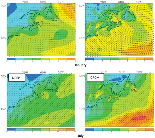
Compared with NCEP reanalyses, the surface winds simulated by the CRCM are northwesterly in winter and westerly in summer. Consistent with the SAT spatial pattern, the CRCM simulation also shows an ability to capture the details of the GSL surface winds (Fig. 3). In January, SST is relatively warm due to the energy transported from the Atlantic Ocean through Cabot Strait, and the planetary atmospheric boundary layer is relatively unstable. Therefore, the sea surface wind speed in the GSL is significantly stronger than over the nearby land (Fig. 3). However, the wind speed along coastal areas is similar to the wind speed over land, suggesting the impacts of sea ice, with heat flux and drag coefficient fields that are similar to those used when the CRCM computes wind speed over land. A similar pattern can also be seen over the Bay of Fundy. However, the maximum wind in these regions is weak in the NCEP reanalysis data because of its coarse resolution as shown in Guo et al. (2013), suggesting a shortcoming (bias) when using NCEP reanalyses to force high-resolution coastal ocean models.

c Sea Ice

Sea ice is an important component of the GSL. When ice forms, it influences the salinity through brine rejection, and when ice melts it causes surface freshening. In addition, sea ice can prevent (or significantly modify) the exchange of heat, moisture, and momentum between the atmosphere and the ocean. In particular, the main effect of sea ice is to reduce the surface wind associated with a storm by reducing the momentum exchange between the atmosphere and the surface water (Long & Perrie, 2012). Sea ice can also impose a drag on the ocean currents flowing beneath it; however, these effects are small because the velocity of the ice is generally much less than that of the wind.

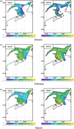
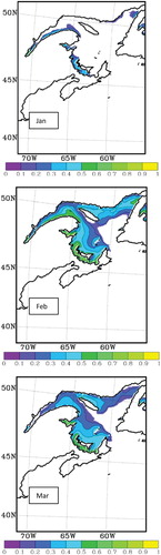
At the scale of the GSL, comparison between the model simulations and 25 km × 25 km National Snow and Ice Data Center (NSIDC) data (Peng, Meier, Scott, & Savoie, 2013) shows that CANOPA reproduces the overall observed sea-ice concentrations well (Fig. 4). In January, sea ice forms along the shallow north and west coasts of the GSL; maximum ice concentrations can be seen in the Strait of Belle Isle, the estuary of the St. Lawrence River, and along the west coast of the GSL. However, the eastern half of the GSL remains ice free because of the warm water inflow from the North Atlantic. In February and March, the GSL is largely covered with sea ice. The maximum ice concentration occurs near Prince Edward Island, whereas the ice concentration near Cabot Strait is relatively small (Fig. 4). In comparison, the simulation by CANOPA slightly underestimates the ice concentration along the west coast of Newfoundland in March, suggesting that it may overestimate the water inflow along the eastern portion of Cabot Strait, but overestimates the ice concentration in January and February. In these winter months, sea ice forms mainly in shallow water, and the impacts of the water inflow along the Cabot Strait are relatively small. The overestimated sea ice in January and February may be related to overestimated surface heat loss in the GSL.

Fig. 4 Monthly ice concentration (colour bar: fractional surface area of all types of ice) from NSIDC data (left panels) and the model simulation (right panels) , averaged over the 1970–1999 period: (a) January, (b) February, and (c) March.

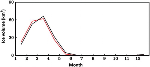
In addition, the CANOPA simulation of ice volume is generally in agreement with Canadian Ice Service data (Fig. 5) as reported by Drinkwater, Pettipas, Bugden, and Langille (1999). Specifically, both observations and model simulation results show that maximum ice volume occurs in March. Thereafter, it rapidly decreases in April, and the GSL is almost ice free by May. In terms of a detailed comparison, CANOPA slightly overestimates the observed ice volume during January and February and underestimates the ice volume in March and April (Fig. 5).

Fig. 5 Monthly ice volume for observations (black) and simulation (red), averaged over the 1970–1999 period.

d Sea Surface Temperature

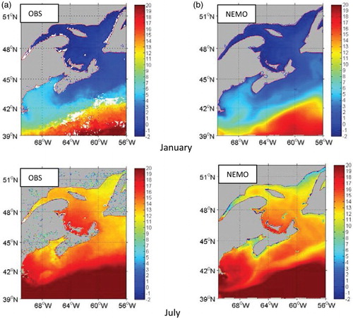
The simulated SST from CANOPA is compared with approximately 0.04° × 0.04° Advanced Very High Resolution Radiometer (AVHRR) satellite data (Kilpatrick, Podesta, & Evans, 2001) in Fig. 6. Because the GSL waters are surrounded by land, these waters are in close contact with the air from nearby land, in particular in the northwest GSL. In January, the SAT over land is typically below −12°C (Fig. 2), and northwesterly winds dominate the region. During this season, the cold air rapidly cools the water surface in the northwest GSL, and sea ice forms rapidly because the SST is already near the freezing point (Fig. 4). Meanwhile, the surface water in the eastern GSL is relatively warm, compared with the northwest GSL, due to water inflow along the eastern part of Cabot Strait (Fig. 6). However, in July, the air temperature over land is warmer than over the GSL, and the SST in the western GSL is relatively warmer than that of the eastern GSL. In addition, the SST near the Strait of Belle Isle is slightly colder than in the western GSL because of the cold water inflow from the Strait of Belle Isle. Overall, comparisons between the model simulations and the satellite data show that CANOPA reproduces SST estimates well in the GSL. However, the model overestimates SST along the west coast of Newfoundland in January and underestimates SST in the western GSL in July, particularly near the Strait of Belle Isle, and coastal waters near Newfoundland (Fig. 6). The approximately 1°C biases may be related to the errors in surface heat flux and transport along the south coast of Newfoundland. Moreover, the discrepancies may be related to the fact that SSTs derived from AVHRR data are the skin temperature of the ocean surface, whereas the model-simulated SSTs are the water temperatures estimated at the model level, which is 3 m. For monthly time scales, shown in Fig. 6, the offset between these two temperature fields is approximately −0.3°C (Donlon et al., 2002).

Fig. 6 Sea surface temperature (°C) in January (upper panels) and July (lower panels) for (a) AVHRR satellite observations and (b) simulation, averaged over the 1980–2009 period.

e Vertical Structures of Water Temperature and Salinity

The simulated vertical profiles of water temperature averaged over 1980 to 2009 are compared with observations from the Bedford Institute of Oceanography archive in Figs 7 and 8, as a time series over the 12-month annual cycle. This archive includes data from the well-known Atlantic Zone Monitoring Program (AZMP; for a description see http://www.meds-sdmm.dfo-mpo.gc.ca/isdm-gdsi/azmp-pmza/index-eng.html). In the central GSL, Fig. 7 shows that the vertical structure of water temperature varies from a two-layer system in winter to a three-layer system in summer. In winter when the GSL is covered with sea ice, water temperature in the upper layer is near freezing, but deeper water is relatively warm. In summer, the upper layer is stratified because of increased surface heat flux. The cold water remnant still exists between the warm waters at the surface and the bottom (Fig. 7). Meanwhile, near Cabot Strait, Fig. 8 suggests that the shallow water is well mixed in winter, and the water temperature is below zero from the surface to the bottom. In summer, the water is stratified, with the water temperature gradually decreasing from the surface to the bottom.

Fig. 7 Time series over the annual cycle, for water temperature (°C; upper panels) and salinity (lower panels) at (60.6333°W, 48.48333°N) comparing observations (left panels) and simulation results (right panels). Numbers on the x-axes indicate months of the year. The location is indicated in Fig. 1.

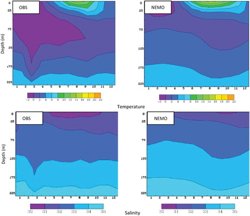
Fig. 8 Time series over the annual cycle for water temperature (°C; upper panels) and salinity (lower panels) at (60.9833°W, 47.0333°N) for observations (left panels) and simulation results (right panels). The location is indicated in Fig. 1.

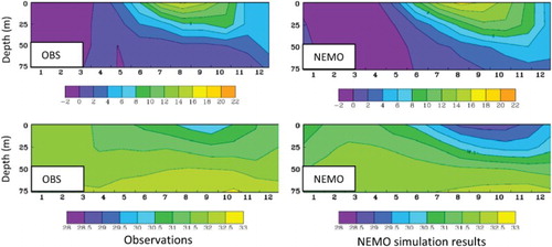
For the two stations, comparisons between the model simulations and observations show that CANOPA can reproduce the vertical structure of water temperature but underestimates the CIL compared with observations (Fig. 7). Moreover, the model fails to capture the detailed annual cycle observed for the deep water temperature. Underestimates in the CIL, as well as the simulation bias shown in the annual cycle of deep water temperature in Fig. 7, may be related to weak surface mixing, which results in underestimates of the transport of cold surface water into the deep ocean.

However, the water salinity is stratified with fresher water near the surface and more saline water near the bottom. Water salinity in the upper layer in winter is relatively high, compared with water salinity in summer (Figs 7 and 8). Although CANOPA is able to capture the overall observed vertical structure, it overestimates salinity in the central GSL (Fig. 7). For the observational station near Cabot Strait, CANOPA overestimates salinity in winter but underestimates salinity in summer (Fig. 8). Clearly, there are biases in the simulated annual cycle of water salinity. On average, CANOPA overestimates salinity by about 0.3.

4 Impacts of climate change

a Surface Air Temperature

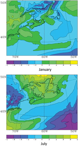
Under the A1B climate change scenario, the land warms faster than the ocean (Fig. 9). The maximum warming in winter is located in northern Quebec, with a maximum above 6°C, as a result of the positive feedback of reduced sea ice and snow in winter. On average, the winter warming over the GSL is about 2°–3°C, with maximum warming located near coastal areas. In addition, the warming near Cabot Strait is relatively weak (<2.5°C) because of Atlantic water inflow through Cabot Strait. In summer, the climate change related to SAT is dominated by the land effect because its heat capacity is smaller than that of water. The warming over the GSL gradually decreases from the western portion of the GSL to the eastern potion. The maximum warming occurs along the west coast with a maximum of about 2°–2.8°C.

Fig. 9 Differences in surface air temperature (°C) in January (upper panel) and July (lower panel) between the 2069–2040 and 1970–1999 periods.

b Surface Wind Speed

There is a strong seasonal variation in the changes of surface wind speed. Climatologically, the land surface is colder than the ocean surface in winter but warmer in summer. Moreover, simulations related to climate change suggest that the land surface warms faster than the ocean surface in a warmer climate (Fig. 9). This warming pattern can reduce the temperature gradient along the coast of the GSL in winter but increase the temperature gradient in summer. In January, the decreased baroclinicity associated with the weakening temperature gradient leads to slight decreases in wind speed over the GSL (Long, Perrie, Gyakum, Laprise, & Caya, 2009), in particular along the north coast of the GSL (Fig. 10). In July, the increased baroclinity significantly increases the wind speed over the GSL. The maximum increase occurs over the central GSL with an amplitude above 0.4 m s⁻¹ (about 15%).

Fig. 10 Differences in 10 m wind speed (m s⁻¹) in January (upper panel) and July (lower panel) between the 2069–2040 and 1970–1999 periods.

c Sea Ice

Under the A1B climate change scenario, ice volume in March steadily decreases from about 80 km³ in the 1980s to near zero by 2069 (Fig. 11), and there is a significant decrease in ice cover, as shown in Figs 4 and 12. Surface warming in the GSL delays ice formation in winter, such that the GSL is largely ice free in January except along the coast in the western portion of the Gulf. In addition, no sea ice can be seen in the eastern portion of the GSL in February or March. In contrast to the current ice climatology, shown in Fig. 4, the ice cover is greater in February than March from 2040 to 2069, suggesting an earlier onset of ice melt in the warmer A1B climate change scenario (Fig. 12).

Fig. 11 Time series of ice volume (km³) in March in the Gulf of St. Lawrence.

Fig. 12 Monthly ice concentration (colour bar: fractional surface area of all types of ice), averaged for the 2040–2069 period.

d Sea Surface Temperature and Salinity

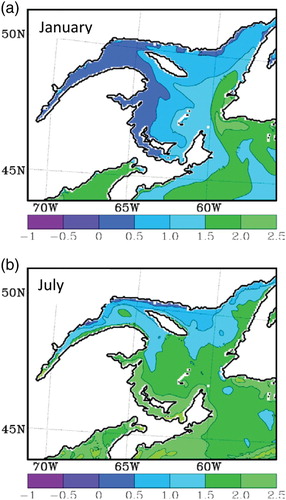
The effects of climate change on SST are dominated by the influence of Atlantic water inflow along the eastern Cabot Strait (Fig. 13). In January, the maximum SST increases are located near eastern Cabot Strait, with qualitative amplitudes of approximately 1.5°–2.5°C. Overall, the increases in SST gradually decrease from east to west. In particular, there is no significant change along the coast of the GSL in January, consistent with trends in sea-ice patterns suggested in Fig. 12. Moreover, the coastal area of weak SST warming in January is broader than the area of notable ice concentration, suggesting that horizontal advection plays a role. However, in July, the maximum increase in SST is also located in the western GSL, because of the maximum increase in SAT in the region, influenced by coastal land processes. The changes are limited along the north coast of the GSL, which may be related to enhanced upwelling associated with the increased wind speed, which offsets surface warming.

Fig. 13 Differences in sea surface temperature (^oC) between the 2040–2069 and 1980–2009 periods in (a) January and (b) July.

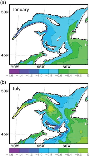
Under the A1B climate change scenario, this study suggests that surface water in the GSL simulated by CANOPA will become fresher (Fig. 14). The maximum decreases in surface salinity are located along western coastal areas because of increased river runoff (Lambert et al., 2013). In January, the salinity decrease is about −0.8 along the northern and western coasts of the GSL and about −0.4 along the eastern GSL. Moreover, no significant changes in surface salinity can be seen in the Atlantic. Compared with changes in January, the changes in surface salinity in July are relatively weaker over the northwestern coast of the GSL, because of enhanced vertical mixing associated with the increased wind speed (Fig. 10), and stronger over southern areas of the GSL, such as around Prince Edward Island and the Scotian Shelf, where wind increases are smaller.

Fig. 14 Differences in sea surface salinity between the 2040–2069 and 1980–2009 periods in (a) January and (b) July.

e Vertical Profiles of Water Temperature and Salinity Anomalies

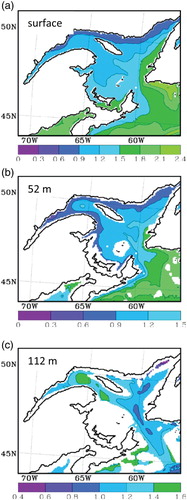
In the warmer A1B climate, the GSL annual water temperature will increase at all depths (Fig. 15). The maximum increase occurs near the surface, where it reaches about 1.5°–1.8°C along the west coast of Newfoundland and about 0.6°–0.9°C along the north coast of the GSL. The temperature increases at 52 m depth are similar to increases at the surface but slightly weaker. They vary from about 0.3°C along the north coast to about 0.9°C along eastern areas of the GSL. However, the increases are a little stronger at 112 m depth, suggesting the impacts of water inflow through the Laurentian Channel. The changes are about 1.0°C in the central and eastern Laurentian Channel and about 1.2°C in the west. Moreover, compared with the upper layer, the changes at 112 m are relatively uniform (Fig. 15).

Fig. 15 Differences in annual water temperature (°C) between the 2040–2069 and 1980–2009 periods at (a) the surface, (b) 52 m, and (c) 112 m..

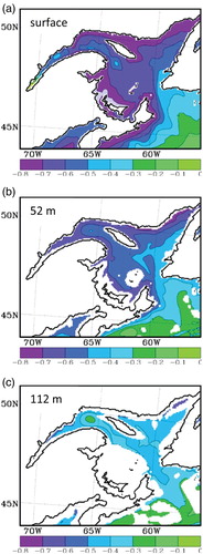
In a warmer climate, the water salinity will decrease during the 2040–2069 period compared with present climatology (Fig. 16). The maximum decreases occur near the surface, where the difference is about −0.7 in the west and −0.5 in the east. The changes at 52 m are slightly weaker than at the surface, about −0.6 in the west and −0.4 along the east coast of Newfoundland. The weakest change occurs near the bottom, about −0.4 over the entire region.

Fig. 16 Differences in annual water salinity between the 2040–2069 and 1980–2009 periods at (a) the surface, (b) 52 m, and (c) 112 m.

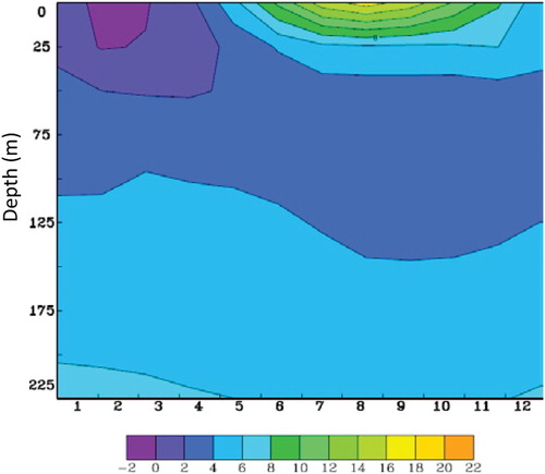
Because the CIL is the habitat of many fish stocks at various stages of their life cycles, it is important to understand the changes that might occur in a warmer climate. Figure 17 shows the vertical profile of water temperature in the central GSL. A cold layer can still be seen at 25–100 m during the 2040–2069 period, but it is about 1°C warmer than in the present climate (Fig. 7). In addition, the vertical profile of water salinity shows a slight freshening although there is no significant change in vertical stratification. Moreover, there are significant seasonal variations in the surface layers (Figs 13 and 14), whereas the seasonal variations are relatively weak near the bottom (figures not shown).

Fig. 17 Time series of water temperature (°C) at 60.6333°W, 48.48333°N, averaged over the 2040–2069 period. The location is indicated in Fig. 1.

5 Concluding discussion

The CRCM is used to downscale simulations from the CGCM3 to provide surface forcing for a high-resolution coastal ocean model (CANOPA). The CGCM3 climate change simulation follows the A1B scenario described by Forster et al. (2007). The CRCM integration is conducted for the 1970–2069 period. We verify that the CRCM is able to reproduce the large-scale patterns of SAT and wind suggested in the NCEP reanalyses datasets. Moreover, the CRCM also provides detailed estimates for the distributions of SAT and wind speed because of a more accurate representation of the coastline.

Driven by CRCM outputs from a 100-year climate change simulation, CANOPA is shown to be able to consistently reproduce the basic patterns in sea ice, SAT, and salinity (qualitatively), as reported in accepted reanalysis and observational datasets (Drinkwater et al., 1999; Kilpatrick et al., 2001). Compared with observations, CANOPA captures the observed seasonal variations in ice cover and volume. For example, both observations and the CANOPA simulations show maxima in ice volume and ice cover in March. Compared with satellite data, CANOPA reproduces the observed climatological SST spatial variability in the GSL well. However, it slightly overestimates SST along the west coast of Newfoundland in January and underestimates SST in the western GSL in July. Although CANOPA reproduces the qualitative features of the vertical structures in water salinity and temperature, and also suggests a cold layer at 25–100 m depth in the central GSL, it underestimates the observed CIL.

Under the A1B climate change scenario, changes in SAT show a seasonal variation. In winter, because of the positive feedback of snow and ice, the maximum warming is located in northern Quebec, which reduces the meridional temperature gradient and baroclinicity. In summer, the warming is dominated by land–sea contrast, when the maximum warming occurs over land, which enhances the temperature gradient and baroclinicity along coastal areas. Over the GSL, CRCM simulations suggest that the increase in winter SAT is about 2°–3°C with maximum warming located along coastal areas, although the warming near Cabot Strait is relatively weak. In summer, the maximum warming is along the west coast of the GSL, and it gradually decreases from west to east. In winter, there is a decrease in wind speed in the GSL because of the weakened baroclinicity. In contrast, enhanced baroclinicity in summer significantly increases the wind speed in the region.

The CANOPA simulations suggest significant changes in sea ice, water temperature, and salinity. Because of the increases in the SAT, the GSL is largely ice free in January, and the ice volume in March steadily decreases from about 80 km³ in the 1980s to near zero in 2069. Moreover, because of the effects of Atlantic inflow through Cabot Strait, the maximum SST increases in winter are located near the eastern part of the GSL with qualitative amplitudes of about 1.5°–2.5°C; there is no significant change along the north and west coasts of the GSL. However, there is also a maximum SST increase in the western GSL in July because of the maximum increase in SAT in the region. In addition, the waters of the GSL will become fresher in the future because of increased river runoff. The maximum decreases in surface salinity occur near coastal areas, while decreases in the eastern GSL are relatively weak. Compared with the present climate, the CIL is significantly weaker during the 2040–2069 period than during the 1980–2009 period. However, when discussing the magnitude of possible changes it should be noted that these results are qualitative, and more studies are needed to address the uncertainties associated with model internal variability and inter-model variability.

Acknowledgements

We thank DFO's Climate Change Science Initiative and the Aquatic Climate Change Adaptation Services Program (ACCASP) for supporting this work. The authors also thank Michel Giguere in Ouranos for his support in setting up CRCM3.7 on the Bedford Institute of Oceanography's Linux cluster and two anonymous reviewers for comments that improved the manuscript.

Disclosure statement

No potential conflict of interest was reported by the authors.

References

- Bouillon, S., Morales Maqueda, M. A., Legat, V., & Fichefet, T. (2009). An elastic-viscous-plastic sea ice model formulated on Arakawa B and C grids. Ocean Modelling, 27, 174–184. doi:10.1016/j.ocemod.2009.01.004
- Brickman, D., & Drozdowski, A. (2012). Development and validation of a regional shelf model for Maritime Canada based on the NEMO-OPA circulation model. Canadian Technical Report of Hydrography and Ocean Sciences. Retrieved from http://www.dfo-mpo.gc.ca/Library/347377.pdf
- Caya, D., & Biner, S. (2004). Internal variability of RCM simulations over an annual cycle. Climate Dynamics, 22, 33–46. doi: 10.1007/s00382-003-0360-2
- Caya, D., & Laprise, R. (1999). A semi-Lagrangian semi-implicit regional climate model: The Canadian RCM. Monthly Weather Review, 127, 341–362. doi: 10.1175/1520-0493(1999)127<0341:ASISLR>2.0.CO;2
- Donlon, C. J., Minnett, P. J., Gentemann, C., Nightingale, J., Barton, I. J., Ward, B., & Murray, M. J. (2002). Toward improved validation of satellite sea surface skin temperature measurements for climate research. Journal of Climate, 15, 353–369. doi: 10.1175/1520-0442(2002)015<0353:TIVOSS>2.0.CO;2
- Drinkwater, K. F., Pettipas, R. G., Bugden, G. L., & Langille, P. (1999). Climatic data for the Northwest Atlantic: A sea ice database for the Gulf of St. Lawrence and the Scotian Shelf. Canadian Technical Report of Hydrography and Ocean Sciences. Retrieved from http://www.dfo-mpo.gc.ca/Library/230707.pdf
- Fichefet, T., & Morales Maqueda, M. A. (1997). Sensitivity of a global sea ice model to the treatment of ice thermodynamics and dynamics. Journal of Geophysical Research, 102, 12,609–12,646. doi:10.1029/97JC00480
- Forster, P., Ramaswamy, V., Artaxo, P., Berntsen, T., Betts, R., Fahey, D. W., … Van Dorland, R. 2007. Changes in atmospheric constituents and in radiative forcing. In S. Solomon, D. Qin, M. Manning, Z. Chen, M. Marquis, K. B. Averyt, M. Tignor and H. L. Miller (Eds.), Climate change 2007: The physical science basis. Contribution of Working Group I to the fourth assessment report of the intergovernmental panel on climate change (pp. 129–234). Cambridge, UK: Cambridge University Press.
- Galbraith, P. S. (2006). Winter water masses in the Gulf of St. Lawrence. Journal of Geophysical Research, 111, C060222. doi:10.1029/2005JC003159
- Guo, L., Perrie, W., Long, Z., Joel, C., Zhang, Y., & Huang, A. (2013). Dynamical downscaling over the Gulf of St. Lawrence using the Canadian Regional Climate Model. Atmosphere-Ocean, 51, 265–283. doi:10.1080/07055900.2013.798778
- Han, G., Loder, J., & Smith, P. (1999). Seasonal-mean hydrography and circulation in the Gulf of St. Lawrence and on the eastern Scotian and southern Newfoundland shelves. Journal of Physical Oceanography, 29, 1279–1301. doi: 10.1175/1520-0485(1999)029<1279:SMHACI>2.0.CO;2
- Kain, J. S., & Fritsch, J. M. (1990). A one-dimensional entraining/detraining plume model and application in convective parameterization. Journal of the Atmospheric Sciences, 47, 2784–2802. doi: 10.1175/1520-0469(1990)047<2784:AODEPM>2.0.CO;2
- Kalnay, E., Kanamitsu, M., Kistler, R., Collins, W., Deaven, D., Gandin, L., … Joseph, D. (1996). The NCEP/NCAR 40-year reanalysis project. Bulletin of the American Meteorological Society, 77, 437–471. doi: 10.1175/1520-0477(1996)077<0437:TNYRP>2.0.CO;2
- Kilpatrick, K. A., Podesta, G. P., & Evans, R. (2001). Overview of the NOAA/NASA Advanced Very High Resolution Radiometer Pathfinder algorithm for sea surface temperature and associated matchup database. Journal of Geophysical Research, 106(C5), 9179–9197. doi: 10.1029/1999JC000065
- Lambert, N., Chassé, J., Perrie, W., Long, Z., Guo, L., & Morrison, J. (2013). Projection of future river runoffs in eastern Atlantic Canada from global and regional climate models. Canadian Technical Report of Hydrography and Ocean Sciences. Retrieved from http://dfo-mpo.gc.ca/Library/349262.pdf
- Laprise, R., Caya, D., Frigon, A., & Paquin, D. (2003). Current and perturbed climate as simulated by the second-generation Canadian Regional Climate Model (CRCM-II) over northwestern North America. Climate Dynamics, 21, 405–421. doi: 10.1007/s00382-003-0342-4
- Large, W. G., & Yeager, S. G. (2008). The global climatology of an interannually varying air-sea flux data set. Climate Dynamics, 33, 341–364. doi: 10.1007/s00382-008-0441-3
- Levitus, S. (1982). Climatological Atlas of the World Ocean. NOAA Prof. Paper 13, US Government Printing Office, Washington DC.
- Long, Z., & Perrie, W. (2012). Air-sea interactions during an Arctic storm. Journal of Geophysical Research, 117, D15103. doi:10.1029/2011JD016985
- Long, Z., Perrie, W., Gyakum, J., Laprise, R., & Caya, D. (2009). Scenario changes in the climatology of winter midlatitude cyclone activity over eastern North America and the northwest Atlantic. Journal of Geophysical Research, 114, D12111. doi:10.1029/2008JD010869
- Madec, G., Delecluse, P., Imbard, M., & Lévy, C. (1998). OPA 8.1 ocean general circulation model reference manual, No. 11. Note du Pôle de modélisation, Institut Pierre-Simon Laplace (IPSL), France.
- McFarlane, N. A., Boer, G. J., Blanchet, J. P., & Lazare, M. (1992). The Canadian Climate Centre second generation general circulation model and its equilibrium climate. Journal of Climate, 5, 1013–1044. doi: 10.1175/1520-0442(1992)005<1013:TCCCSG>2.0.CO;2
- Mellor, G. L., and Yamada, T. (1982). Development of a turbulent closure model for geophysical fluid problems. Reviews of Geophysics, 20, 851–875. doi: 10.1029/RG020i004p00851
- Mesinger, F., DiMego, G., Kalnay, E., Mitchell, K., Shafran, P. C., Ebisuzaki, W., … Shi, W. (2006). North American regional reanalysis. Bulletin of the American Meteorological Society, 87, 343–360. doi: 10.1175/BAMS-87-3-343
- Paquin, D., & Caya, D. (2001). New convection scheme in the Canadian Regional Climate Model. In H. Ritchie (Ed.), Research activities in atmospheric and oceanic modelling. WMO/TD -987, Rep 30, 7.14–7.15., Geneva.
- Peng, G., Meier, W., Scott, D., & Savoie, M. (2013). A long-term and reproducible passive microwave sea ice concentration data record for climate studies and monitoring. Earth System Science Data, 5, 311–318. doi:10.5194/essd-5-311-2013
- Randall, D. A., Wood, R. A., Bony, S., Colman, R., Fichefet, T., Fyfe, J., … Taylor, K. E. (2007). Climate models and their evaluation. In S. Solomon, D. Qin, M. Manning, Z. Chen, M. Marquis, K. B. Averyt, M. Tignor, & H. L. Miller (Eds.), Climate change 2007: The physical science basis. Contribution of Working Group 1 to the fourth assessment report of the intergovernmental panel on climate change (pp. 589–662). Cambridge, UK: Cambridge University Press.
- Saucier, J. F., Roy, F., Gilbert, D., Perrin, P., & Ritchie, H. (2003). Modeling the formation and circulation processes of water masses and sea ice in the Gulf of St. Lawrence, Canada. Journal of Geophysical Research, 108(C8), 3269. doi: 10.1029/2000JC000686
- Smith, G. C., Saucier, F. J., & Staub, D. (2006). Formation and circulation of the cold intermediate layer in the Gulf of Saint Lawrence. Journal of Geophysical Research, 111, C06011. doi:10.1029/2005JC003017