Statistical Projections of Ocean Climate Indices off Newfoundland and Labrador

ABSTRACT

Present global climate models (GCMs) are unable to provide reliable projections of physical oceanographic properties on the continental shelf off Newfoundland and Labrador. Here we first establish linear statistical relationships between oceanographic properties and coastal air temperature based on historical observations. We then use these relationships to project future states of oceanographic conditions under different emission scenarios, based on projected coastal air temperatures from global (Canadian Earth System Model, version 2 (CanESM2), Geophysical Fluid Dynamics Laboratory's Earth System Model, version 2M (GFDL-ESM2M)) and regional (Canadian Regional Climate Model (CRCM)) climate models. Estimates based on CanESM2 agree reasonably well with observed trends, but the trends based on two other models result in substantial underestimates. Projected trends are closer to observations under a high emission scenario than under median-level emission scenarios. Over the next 50 years, the increases in projected sea surface temperature off eastern Newfoundland (Station 27) range from 0.4° to 2.2°C. The increases in bottom ocean temperature over the Newfoundland and Labrador Shelves range from 0.4° to 2.1°C. The area of the cold intermediate layer (<0°C) on the Flemish Cap (47°N) section is projected to decrease by 9–35% of the 1981–2010 average. The decline in sea-ice extent off Newfoundland and Labrador ranges from 20 to 77% of the average (0.4–1.5 × 10⁵ km²), and the reduction in the number of icebergs at 48°N off Newfoundland ranges from 30% to nearly 100% of the norm at this latitude. Despite differences among the models and scenarios, statistical projections indicate that conditions in this region will reach or exceed their maxima (sea surface temperature, bottom ocean temperature) and reach or fall below their minima (sea-ice extent, number of icebergs) that were observed during the course of monitoring activities over the past 30–60 years, possibly as early as 2040. We note, however, that the statistical relationships based on historical data may not hold in the future because of the changing influence of input from Arctic waters and because of large uncertainties in projected air temperatures from GCMs.

RÉSUMÉ

[Traduit par la redaction] Les modèles actuels du climat du globe sont incapables de fournir des projections fiables des propriétés océanographiques physiques de la région du plateau continental au large de Terre-Neuve et du Labrador. Nous établissons d'abord une relation statistique linéaire entre les propriétés de l'océan et la température de l'air côtier, sur la base d'observations historiques. Nous utilisons ensuite ces relations, afin de prévoir l’état futur des conditions océanographiques, à partir des températures de l'air prévues, en variant les scénarios d’émissions des modèles globaux du climat (le modèle canadien du système terrestre, version 2 [CanESM2] et le modèle du système terrestre du Geophysical Fluid Dynamics Laboratory, version 2M [GFDL-ESM2M]) et du Modèle régional canadien du climat (MRCC). Les estimations issues du CanESM2 concordent raisonnablement bien avec les tendances observées, mais les deux autres modèles sous-estiment considérablement les tendances. Les tendances prévues s'avèrent plus près des observations pour un scénario d’émissions élevées que pour les scénarios qui tiennent les émissions sous la médiane. Sur les 50 prochaines années, l'augmentation des températures prévues de la surface de la mer à l'est de Terre-Neuve (station 27) va de 0,4 à 2,2°C. L'augmentation de la température des eaux du fond marin des plateaux de Terre-Neuve et du Labrador va de 0,4 à 2,1°C. La partie de la couche intermédiaire froide (<0°C) située dans la zone du bonnet Flamand (47° N) est censée subir une diminution de 9 à 35% de sa moyenne, calculée entre 1981 et 2010. La réduction de l’étendue de la glace de mer au large de Terre-Neuve et du Labrador va de 20 à 77% de la moyenne (0,4 × 10⁵ à 1,5 × 10⁵ km²), et la diminution du nombre d'icebergs à 48° N, au large de Terre-Neuve, va de 30% à près de 100% de la normale à cette latitude. Malgré les différences observées entre les modèles et les scénarios, les projections statistiques indiquent que les conditions dans cette région atteindront ou dépasseront les maximums (températures à la surface et au fond de la mer) et atteindront ou tomberont sous les minimums (étendue de la glace de mer, nombre d'icebergs) qui ont été observés dans le cadre d'activités de surveillance au cours des 30 à 60 dernières années, et ce, possiblement dès 2040. Nous notons, toutefois, que les relations statistiques fondées sur les données historiques pourraient ne pas s'appliquer à l'avenir, en raison de l’évolution de l'influence des facteurs relatifs aux eaux arctiques et à cause des grandes incertitudes minant les températures de l'air que prévoient les modèles globaux du climat.

KEYWORDS:

• climate change
• statistical projections
• ocean climate indices
• temperature
• sea-ice extent
• iceberg

1 Introduction

Present global climate models (GCMs) are unable to resolve many oceanic processes (e.g., mesoscale and sub-mesoscale eddies) that are important to climate variability and thus may be unable to provide reasonable projections of water properties in many parts of the world ocean, particularly in coastal and shelf regions. This limitation is acutely evident in the subpolar Northwest Atlantic (Fig. 1; e.g., Loder and van der Baaren, 2013). A solution to this limitation is to develop dynamic downscaling based on regional climate models (RCMs; e.g., Guo et al., 2013). However, such downscaled RCMs are not always available, and even when available they may not resolve some important regional oceanic processes. An alternative, then, is to establish statistical downscaling based on historical observations.

Fig. 1 Map showing the study region. Station 27 (red diamond), the Flemish Cap transect (black line), and the area with the fall bottom temperature data (dashed lines) are indicated.

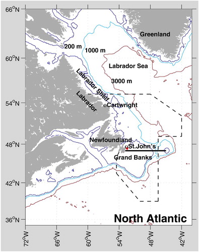
The subpolar Northwest Atlantic (Fig. 1), including the Newfoundland and Labrador Sheves, is directly influenced by the Arctic outflow from the Canadian Arctic Archipelago (CAA) and is both important in and sensitive to global climate variability and change. In winter and spring the waters off Newfoundland and Labrador are covered with pack ice. The concentration of ice varies considerably, depending on the strength and direction of the wind and air temperature. Most of the pack ice off Newfoundland's northern and eastern shores originates off Labrador. The pack ice advances southward until around April when the rate of melting overtakes the rate of advance which results in a northward retreat of the ice edge. Icebergs originating from Greenland glaciers are common in the waters off Newfoundland in spring and early summer. A subsurface layer of cold water exists in summer, which is referred to as the cold intermediate layer (CIL). It has a characteristic thickness of 100–200 m, minimum summer temperatures of −1.0° to −1.5°C, and extends 200–300 km from the coast. On the Newfoundland and Labrador Shelves, regional physical oceanographic properties exhibit significant variations at interannual, decadal, and secular scales. It has been demonstrated that regional oceanographic properties off eastern Canada are closely linked to meteorological forcing on interannual and decadal scales (e.g., Deser, Holland, Reverdin, & Timlin, 2002; Han, 2005, 2007; Petrie, 2007), specifically air temperatures and the North Atlantic Oscillation (NAO), the dominant atmospheric mode in the North Atlantic (Hurrell, 1995). In addition, as a result of the proximity of the Newfoundland and Labrador Shelves to the North Atlantic subpolar gyre, the region is strongly affected by the Labrador Current, which is closely linked to the NAO (Han et al., 2010), and by the interaction of the subpolar and subtropical gyres (Loder, Petrie, & Gawarkiewicz, 1998; Han, Chen, & Ma, 2014). On multi-decadal scales, the Atlantic Multi-decadal Oscillation (AMO; Schlesinger, 1994) may play a role in regional oceanographic changes.

The Newfoundland and Labrador Shelves host a highly productive marine ecosystem. The distribution of zooplankton and larval fish are closely related to changes in ocean temperatures and circulation (Pepin and Helbig, 1997; Han and Kulka, 2009; Pepin, Han, & Head, 2013). Sea-ice extent in spring and winter affects marine navigation, and the timing of ice melt can significantly influence spring bloom and regional productivity (Wu et al., 2007; Zhao, Han, & Wang, 2013; Buren et al., 2014). The presence of icebergs may endanger the operation of offshore platforms and commercial shipping. Therefore, knowledge of when future oceanographic conditions under a changing climate will exceed observations of past conditions collected over the last 30–60 years should allow resource managers, industry, and government policy-makers to anticipate the need for adaptation.

In this study, we use historical oceanographic and meteorological observations to establish statistical empirical linear relationships between oceanographic variables, including sea ice and icebergs, as well as air temperatures. Based on the output of two GCMs, one RCM, and our empirical relationships, we project trends in ocean conditions on the Newfoundland and Labrador Shelves from the present until 2060. Our approach is similar to Rahmstorf's (2007), in which global mean sea level rise is projected from global air temperature rise.

2 Data and method

Historical oceanographic data and ocean climate indices along standard oceanographic sections and at high frequency monitoring sites on the Newfoundland and Labrador Shelves were obtained from the Atlantic Zone Monitoring Program (AZMP; http://www.meds-sdmm.dfo-mpo.gc.ca/isdm-gdsi/azmp-pmza/index-eng.html). Data for broad areas were obtained from regional resource assessment surveys (Colbourne, Craig, Fitzpatrick, Senciall, Stead, & Bailey, 2013). Anomalies in selected oceanographic variables were calculated relative to their means (Table 1) over the standard climatological reference period, 1981–2010. Linear regressions served to establish statistical relationships between the anomalies of ocean variables of interest and those of air temperature at St. John's, Newfoundland (47.62°N, 52.73°W), and Cartwright (53.71°N, 57.04°W), Labrador, as in Han, Colbourne, Pepin, and Tang (2013). The air temperatures at St. John's and Cartwright are from the Adjusted and Homogenized Canada Climate Data (http://www.ec.gc.ca/dccha-ahccd/default.asp?lang=en&n=70E82601-1). Sea-ice extent was available from the Canadian Ice Service (CIS; http://www.ec.gc.ca/glaces-ice/) of Environment Canada and iceberg numbers were provided by the International Ice Patrol of the US Coast Guard (http://www.navcen.uscg.gov/?pageName=IIPHome).

Table 1. Means and standard deviations for the 1981–2010 reference period (SST: sea surface temperature; CIL: cold intermediate layer; BT: bottom temperature). See Fig 1 for locations.

Variable	1981–2010 Mean	Standard Deviation
SST (°C) at Station 27	5.18	0.82
CIL (km^2) at the Flemish Cap transect	26.52	6.63
Fall BT (°C) over the Newfoundland and Labrador Shelves	1.61	0.50
Winter SIE (10^5 km^2)	1.96	0.81
Number of icebergs at 48°N	813	648
NAO (hPa)	20.44	8.77
St. John's air temperature (°C)	5.03	0.84
Cartwright air temperature (°C)	0.05	1.32

The air temperature output of the Canadian Earth System Model, version 2 (CanESM2; an ensemble of five members), the output from the Geophysical Fluid Dynamics Laboratory's Earth System Model, version 2M (GFDL-ESM2M; one member only; Loder and van der Baaren, 2013), and output from the Canadian Regional Climate Model (CRCM; an average of two members; Guo et al., 2013) were used to produce projections for certain oceanographic variables based on the statistical relationships that were established. Differences among members of a model represent the model's internal variability. Both CanESM2 (Chylek, Li, Dubey, Wang, & Lesins, 2011) and GFDL-ESM2M (Dunne et al., 2012) are among the Earth System Models (ESMs) used in the Coupled Model Intercomparison Project, phase 5 (CMIP5; http://cmip-pcmdi.llnl.gov/cmip5). The atmospheric model of the two GCMs has a horizontal grid resolution of about 2.5° and that of the CRCM has a horizontal resolution of 45 km. With respect to the observed global seasonal-cycle climatology (1980–2005), the air temperature error of CanESM2 is slightly smaller than the CMIP5 error and that of GFDL-ESM2M is larger (Flato et al., 2013). The projected air temperature rise during the twenty-first century from CanESM2 is larger than the CMIP5 average and the projection by GFDL-ESM2M is smaller (Collins et al., 2013). The ocean climate variables considered in the analyses include annual-mean sea surface temperature (SST; <5 m depth) at a high frequency monitoring site off eastern Newfoundland (Station 27, located approximately 8 km off St. John's 47.55°N, 52.59°W), the fall bottom temperature (BT) spatially averaged over the Newfoundland and Labrador Shelves during the fall resource assessment surveys (North Atlantic Fisheries Organization Divisions 2J3KLNO), the cross-sectional area of the CIL shelf water <0°C along the Flemish Cap (47°N) section during summer (July), winter (January–March) sea-ice extent (SIE) defined as areas with ≥1/10 coverage off Newfoundland and Labrador south of 55°N (Fig. 1), and the number of icebergs south of 48°N. The data periods are 1950–2010 for Station 27 SST, 1978–2010 for the fall BT, 1951–2011 for the CIL, 1963–2011 for the SIE, and 1983–2011 for the number of icebergs. Iceberg data prior to 1983 are not used to avoid data inconsistency resulting from different iceberg detection methods. Two representative concentration pathways (RCPs), RCP4.5 and RCP8.5, were considered for CanESM2 and GFDL-ESM2M, corresponding to moderate and extreme emissions of CO₂, respectively. In the case of CRCM, which is a downscaled model of CanESM2, only the moderate emission scenario (A1B) was considered. The projected trends are essentially the same for the five members of CanESM2 as are those for the two members of CRCM; therefore, we show the ensemble results only. According to Loder and van der Barren (2013) GFDL-ESM2M and CanESM2 provide approximate lower and higher bounds for projected changes in the Northwest Atlantic among six ESMS they considered.

Using linear regression, the oceanographic variables were then modelled using modelled air temperatures from the GCMs and RCMs from 1970 (or data start year if later than 1970) to 2010 (or 2011). The method was validated by comparing the modelled trends with observed ones. St. John's and Cartwright air temperatures projected by CanESM2, GFDL-ESM2M, and CRCM for the periods 2011–2100 and 2011–2069, along with the linear regression model between observed oceanographic variables and observed air temperatures, were then used to produce statistical projections for SST, BT, CIL, SIE, and iceberg numbers. The linear trends over 2011–2100 and over 2011–2069 were then computed. Finally, projected changes and associated uncertainties for 2011–2060 were calculated by multiplying the linear trends and associated standard errors by 50 years. Note that the values in all the figures are the anomalies relative to the means over the 1981–2010 reference period (Table 1).

3 Results

a SST at Station 27

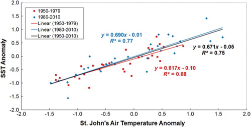
There is a strong positive linear relationship (R² = 0.75, p < 0.01) between the annual-mean SST at Station 27 and the annual-mean air temperature at St. John's from 1950 to 2010 (Fig. 2). When the datasets are divided into two periods (1950–1980 and 1981–2010), the regression coefficients are nearly identical (Fig. 2), suggesting the robustness of the empirical relationship with time. The tri-decadal periods chosen are sufficiently long to minimize the effects of decadal variability. During the latter period several key global climate indices showed larger trends than in the former.

Fig. 2 Scatter diagram between the observed sea surface temperature anomalies (SST, °C) at Station 27 and the observed air temperature anomalies (°C) at St. John's from 1950 to 2010. The lines show the linear fits to the annual-mean observations.

The observed SST at Station 27 has a linear trend of 0.023°C per year over the 1970–2010 period (Table 2). The linear trends of statistically reconstructed SSTs over this period are about 0.021°C per year based on CanESM2 air temperatures under RCP4.5 and RCP8.5, agreeing well with observations (Fig. 3). The trends based on GFDL-ESM2M and CRCM show greater differences (0.004–0.011°C per year) from observations (Table 2).

Fig. 3 Reconstructed SST anomalies (°C) at Station 27 based on simulated air temperature anomalies at St. John's. The air temperatures are the CanESM2 and GFDL-ESM2M output under RCP4.5 and RCP8.5 and the CRCM output under A1B. The straight lines are the linear fits to the SST projections for 2011–2100 or 2011–2070.

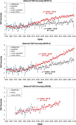
Table 2. Linear trends and associated standard errors.

		A1B	RCP4.5	RCP8.5
	1970–2010
SST (°C y^−1)	Observed	0.023 ± 0.008
	CanESM2	–	0.021 ± 0.003	0.022 ± 0.003
	GFDL-ESM2M	–	0.012 ± 0.005	0.018 ± 0.005
	CRCM	0.019 ± 0.004	–	–
	1978–2010
BT (°C y^−1)	Observed	0.049 ± 0.013
	CanESM2	–	0.034 ± 0.004	0.034 ± 0.004
	GFDL-ESM2M	–	0.012 ± 0.006	0.020 ± 0.006
	CRCM	0.018 ± 0.006	–	–
	1970–2011
CIL (km^2 y^−1)	Observed	−0.211 ± 0.083
	CanESM2	–	−0.178 ± 0.020	−0.191 ± 0.022
	GFDL-ESM2M	–	−0.078 ± 0.033	0.094 ± 0.033
	CRCM	−0.131 ± 0.047	–	–
	1970–2011
SIE (10^5 km^2 y^−1)	Observed	−0.031 ± 0.009
	CanESM2	–	−0.028 ± 0.003	−0.030 ± 0.003
	GFDL-ESM2M	–	−0.012 ± 0.005	−0.015 ± 0.005
	CRCM	−0.020 ± 0.007	–	–
	1983–2011
Icebergs (y^−1)	Observed	−31 ± 14
	CanESM2	–	−25 ± 3	−26 ± 2
	GFDL-ESM2M	–	−9 ± 4	−15 ± 4
	CRCM	−13 ± 4	–	–

The statistically projected SST based on CanESM2 air temperatures shows a greater increase over time, while that based on GFDL-ESM2M output demonstrates a weaker increase and greater variability (Fig. 3). Based on the CanESM2 output, the projected annual-mean SST increase is between 1.0 ± 0.1°C and 2.2 ± 0.1°C by 2060 under RCP4.5 and RCP8.5, respectively. The GFDL-ESM2M projections indicate an increase of about 0.4 ± 0.1°C and 1.1 ± 0.1°C, respectively. The CRCM projected increases are 1.5 ± 0.1°C. Loder et al. (2013) reported an increase of 2°C from an ensemble average of six Intergovernmental Panel on Climate Change (IPCC) atmosphere–ocean general circulation models (AOGCMs) including CanESM2 and GFDL-ESM2M. To put these increases into perspective the 1981–2010 annual mean SST at Station 27 is 5.18°C (Table 1).

b Fall BT Over the Newfoundland and Labrador Shelves

The fall BT over the Newfoundland and Labrador Shelves shows a strong positive linear relationship (R² = 0.59, p < 0.01) with the annual-mean air temperature at Cartwright from 1978 to 2010 (Fig. 4). The observed fall BT over the Newfoundland and Labrador Shelves has a linear trend of 0.049°C per year from 1978 to 2010 (Table 2). The linear trends of the statistically reconstructed BT over this period are 0.034°C per year based on CanESM2 air temperatures, approximately two-thirds of those observed (Fig. 5). The reconstructed trends, based on the GFDL-ESM2M and CRCM air temperatures, are even smaller (0.012° to 0.020°C per year).

Fig. 4 Scatter diagram between the observed fall bottom temperature anomalies (BT, °C) over the Newfoundland and Labrador Shelves and the observed air temperature anomalies (°C) at Cartwright from 1978 to 2010. The line is the linear fit to the observations.

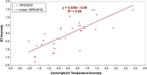
Fig. 5 Reconstructed fall bottom temperature anomalies (BT, °C) over the Newfoundland and Labrador Shelves based on simulated air temperature anomalies at Cartwright. The air temperatures are the CanESM2 and GFDL-ESM2M output under RCP4.5 and RCP8.5 and the CRCM output under A1B. The straight lines are the linear fits to the BT projections for 2011–2100 or 2011–2070.

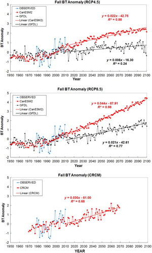
Based on the CanESM2 output, the statistically projected BT increase is 1.1 ± 0.1°C and 2.1 ± 0.1°C by 2060 under RCP4.5 and RCP8.5, respectively (Fig. 5). Based on the GFDL-ESM2M output, BT is projected to rise by 0.4 ± 0.1°C and 1.0 ± 0.1°C, respectively, under RCP4.5 and RCP8.5. The CRCM projected increase is 1.5 ± 0.2°C. The climatological (1981–2010) mean Newfoundland and Labrador Shelves BT is 1.61°C (Table 1).

c CIL Area at the Flemish Cap (47°N) Section

The summer CIL area on the Flemish Cap section has a negative linear relationship (R² = 0.46, p < 0.01) with the winter (January through March) mean air temperature upstream at Cartwright (Fig. 6). A correlation between CIL and winter air temperature was also found in the neighbouring Gulf of St. Lawrence (Galbraith, Hebert, Colbourne, & Pettipas, 2013). When the data are divided into two periods (1951–1980 and 1981–2011) regression coefficients change nearly two-fold (Fig. 6), suggesting that the use of the historical relationship may substantially underestimate future declines in the CIL because of the steep decline in CIL during the last 30 years. Nevertheless, based on the linear relationship for 1951–2011 the general pattern of variation in CIL anomalies along the Flemish Cap section were reconstructed from projected winter air temperatures at Cartwright from 1950 to 2100 (or 2069) (Fig. 7).

Fig. 6 Scatter diagram between the observed CIL area anomalies (km²) at the Flemish Cap section and the observed winter air temperature anomalies (°C) at Cartwright from 1951 to 2011. The line is the linear fit to observations.

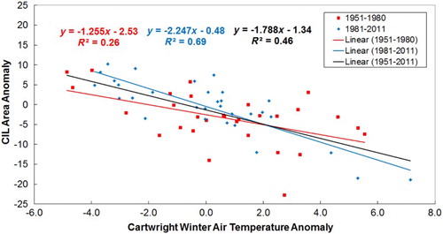
Fig. 7 Reconstructed cold intermediate layer (CIL) area anomalies (km²) along the Flemish Cap transect based on simulated winter air temperature anomalies at Cartwright. The air temperatures are the CanESM2 and GFDL-ESM2M output under RCP4.5 and RCP8.5 and the CRCM output under A1B. The straight lines are linear fits to the CIL projections for 2011–2100 or 2011–2070.

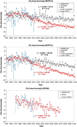
The observed CIL area has a linear trend of −0.211 km² y⁻¹ over the 1970–2011 period (Table 2). The linear trends of the statistically reconstructed CIL area over the period are −0.178 and −0.191 km² y⁻¹ based on the CanESM2 air temperatures for RCP4.5 and RCP8.5, respectively, in general agreement with observations. The trends based on GFDL-ESM2M air temperatures are much weaker, while the CRCM-based trend is about two-thirds of the observed.

By 2060, the projected CIL decreases by 5.4 ± 0.3 km² and 8.6 ± 0.3 km² (20 and 32% of the 1981–2010 mean of 26.52 km²) under RCP4.5 and RCP8.5, respectively, based on CanESM2 output (Fig. 7). The CIL area decreases by 2.3 ± 0.6 km² and 4.8 ± 0.5 km² (9 and 18% of the 1981–2010 mean) under RCP4.5 and RCP8.5, respectively, based on the GFDL-ESM2M output. The CRCM projected decrease is 9.3 ± 1.5 km² (35% of the 1981–2010 mean).

d Winter SIE off Newfoundland and Labrador South of 55°N

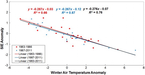
The winter SIE off Newfoundland and Labrador has a high negative linear relationship (R² = 0.76, p < 0.01) with the winter mean air temperature at Cartwright (Fig. 8). A correlation between ice conditions and winter air temperature was also found in the Gulf of St. Lawrence (Galbraith et al., 2013). When the datasets are divided into two periods (1963–1986 and 1987–2011) the regression coefficients are almost the same (Fig. 8), suggesting the robustness of the derived empirical relationship with time. Nevertheless, it may become non-linear in the future.

Fig. 8 Scatter diagram between the observed sea-ice extent (SIE) anomalies (×10⁵ km²) off Newfoundland and Labrador and the observed winter air temperature anomalies (°C) at Cartwright from 1963 to 2011. The line is the linear fit to observations

The observed SIE area has a linear trend of −0.031 × 10⁵ km² y⁻¹ over the 1970–2011 period (Table 2). The linear trends of the statistically reconstructed SIE area over the period are −0.028 × 10⁵ and −0.030 × 10⁵ km² y⁻¹ based on CanESM2 air temperatures under RCP4.5 and RCP8.5, respectively, consistent with observations (Fig. 9). The trends based on the GFDL-ESM2M air temperatures are much smaller, while the CRCM-based trends are about two-thirds of the observed ones.

Fig. 9 Reconstructed sea-ice extent anomalies (SIE) (×10⁵ km²) off Newfoundland and Labrador based on the simulated winter air temperature anomalies at Cartwright. The air temperatures are the CanESM2 and GFDL-ESM2M output under RCP4.5 and RCP8.5 and the CRCM output under A1B. The straight lines are the linear fits to the SIE projections from 2011 to 2100. Note that years with SIE anomalies below −1.96×10⁵ km² are ice free.

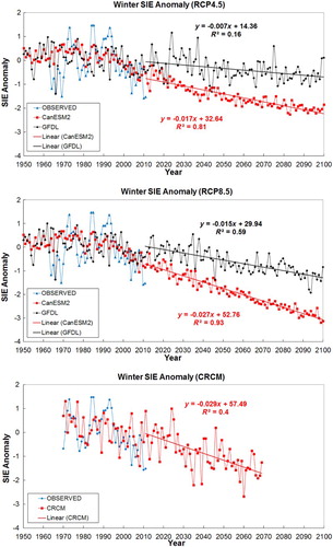
By 2060, the statistically projected SIE decreases are approximately (0.9 ± 0.1) × 10⁵ km² and (1.4 ± 0.1) × 10⁵ km² (46 and 71% of the 1981–2010 mean of 1.96 × 10⁵ km²) under RCP4.5 and RCP8.5, respectively, based on the CanESM2 output (Fig. 9). Projected decreases are of (0.4 ± 0.1) × 10⁵ km² and (0.8 ± 0.1) × 10⁵ km² (20 and 41% of the 1981–2010 mean) under RCP4.5 and RCP8.5, respectively, based on the GFDL-ESM2M output. The CRCM projected decreases are (1.5 ± 0.3) × 10⁵ km² (77% of the 1981–2010 mean). Under RCP8.5 the Newfoundland and Labrador Shelves south of 55°N will essentially become ice free before 2100 when the anomaly falls below −2.77 × 10⁵ km². As a reference, both models project that by 2050 the Arctic Ocean will essentially be ice free in September (Stroeve et al., 2012).

e Number of Icebergs at 48°N off Newfoundland

The number of icebergs at 48°N has a negative linear relationship (R² = 0.40, p < 0.01) with winter mean air temperature at Cartwright (Fig. 10), which represents the weakest of the statistical relationships explored in this analysis.

Fig. 10 Scatter diagram between the observed number of iceberg anomalies at 48°N and the observed winter air temperature anomalies (°C) at Cartwright from 1983 to 2011. The line is the linear fit to observations.

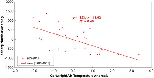
The number of icebergs has a linear trend of −31 per year from 1983 to 2011 (Table 2). The linear trends of the statistically reconstructed iceberg numbers for this period are −25 and −26 per year based on the CanESM2 air temperatures, close to the observed trend (Fig. 11). The trends based on GFDL-ESM2M and CRCM air temperatures are much smaller (−9 to −15 per year).

Fig. 11 Reconstructed iceberg number anomalies at 48°N based on simulated winter air temperature anomalies at Cartwright. The air temperatures are the CanESM2 and GFDL-ESM2M output under RCP4.5 and RCP8.5 and the CRCM output under A1B. The straight lines are the linear fits to the projected number of icebergs from 2011 to 2100. Note that years with iceberg number anomalies below −813 are iceberg free.

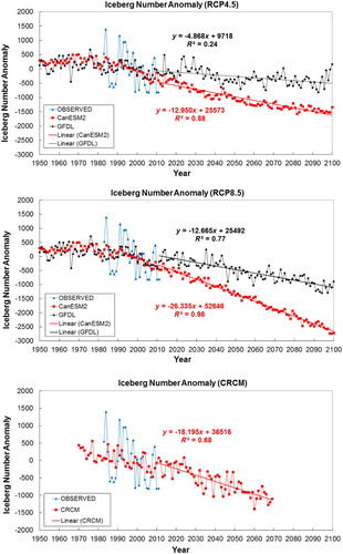
By 2060, the projected decreases in the number of icebergs are 641 ± 25 and 1309 ± 19 (79–161% of the 1981–2010 mean of 813) under RCP4.5 and RCP8.5, respectively, based on the CanESM2 output (Fig. 11). The projected decreases in the number of icebergs are 242 ± 46 and 630 ± 37 (30–77% of the 1981–2010 mean) under RCP4.5 and RCP8.5, respectively, based on the GFDL-ESM2M output. The CRCM projected decrease is 905 ± 81 (111% of the 1981–2010 mean). Note that the production of icebergs may change in the future.

4 Discussion and conclusions

The empirical linear relationships between atmospheric forcing and ocean response have been identified for the Newfoundland and Labrador Shelves. The mechanisms involved in generating them are discussed briefly here. There is a strong link between air temperatures and both SST (R² = 0.75) and SIE (R² = 0.76); this reflects the strong interaction between these environmental metrics at the air–sea interface. The slightly weaker relationship between bottom ocean temperature and air temperature at Cartwright (R² = 0.59) may be attributable, in part, to the time required for temperature fluctuations to propagate from the surface to the bottom but may also be influenced by other processes, such as advection, that can affect ocean temperature at depth. The weaker relationship between air temperature and the area of the CIL (R² = 0.46) may also reflect the time required for intermediate water formation and the processes involved. For example, variability in ocean currents, water column stratification, wind-induced mixing, and cross shelf exchange with slope water all affect the volume of CIL water remaining on the shelf during the summer months. The influence of air temperature on the melting of icebergs (R² = 0.40) is, to a large degree, manifested through its effects on surface and subsurface water temperatures and also on SIE.

Using statistically significant relationships based on historical oceanographic observations and observed air temperatures, five physical oceanographic variables were projected under two RCPs (RCP4.5 and RCP8.5), based on projected air temperatures from two GCMs (CanESM2 and GFDL-ESM2M). Projections were also produced under the A1B emission scenario based on projected air temperatures from the CRCM. The trends in air temperature at St. John's and Cartwright from CRCM and CanESM2 are stronger than the air temperature trends from GFDL-ESM2M. Comparisons with observations show that the estimates based on CanESM2 are in good agreement with the trends observed during the last 50–60 years. The trends based on the two other models substantially underestimate past changes in environmental metrics. The statistically reconstructed trends are closer to the observed ones under the high emission scenario, RCP8.5, than under the median-level emission scenarios (RCP4.5 and A1B).

Over the next 50 years, the projected increases in SST at Station 27 ranges from 0.4° to 2.2°C; the projected increase in BT over the Newfoundland and Labrador Shelves ranges from 0.4° to 2.1°C; the projected decrease in CIL area on the Flemish Cap (47°N) section are 2.3–9.3 km² (9–35% of the 1981–2010 mean); the projected decrease in SIE off Newfoundland and Labrador ranges from 0.4 km² to 1.4 × 10⁵ km² (20–77%); and the decrease in the number of icebergs at 48°N off Newfoundland ranges from 242 (30%) to 1309 (almost no icebergs at this latitude). The statistical models based on CanESM2 reproduce past trends in observations more accurately than the other models, and they also project the largest or close-to-largest trends into the future.

Although the three models predict differing magnitudes of change under the two RCPs and the A1B scenario, they all project increases in ocean temperature throughout the Newfoundland and Labrador region over the next 50 years. Despite differences among the models and scenarios, projections based on statistical downscaling indicate that conditions in this region will reach or exceed the maximum (SST, BT) and reach or fall below the minimum (SIE, number of icebergs) that were observed during monitoring activities over the past 30–60 years, possibly as early as 2040.

The statistical relationships established use historical data and may not hold in the future. In some cases, the established relationships are sensitive to the length of the time series. This sensitivity may be mitigated by including the most recent data or by gaining a greater understanding of the processes that could affect the observed fluctuations in ocean conditions. There are large uncertainties in coastal air temperatures projected by the two GCMs and the CRCM. These uncertainties may be alleviated as climate models improve.

Despite differing levels of uncertainty in the statistical relationships that were used for projections, some important consistencies among variables, models, and RCPs should be noted. In many instances, there are differences between models and RCPs, but these are generally small relative to the magnitude of the underlying residual error. In particular, results based on CanESM2 RCP4.5 and CRCM A1B output are in good agreement not only in their forecasts but also in the reconstructed patterns of variation. In nearly all instances, projections using CanESM2 demonstrate more pronounced changes than those obtained from GFDL-ESM2M, and, as a result, the likelihood of projected changes exceeding the range of past observations or exceeding the underlying residual error differs substantially between the two models. Under most circumstances, projections from CanESM2 exceed the range of past observations (and the residual error) under the more conservative RCP4.5. In contrast, projections using GFDL-ESM2M seldom exceed the range of past observations or residual error under either of the RCPs although they tend to remain close to past extremes (high for temperature, low for SIE and iceberg numbers) for most of the period beyond 2040.

In the short term (approximately a 10-year projection), high temperatures and low CIL area, SIE, and iceberg numbers will continue with significant interannual variability. Over the next few decades it is likely that trends may ease to some degree as the AMO switches from the recent warm phase to a cold phase.

Changes in SIE will have important implications for wind waves reaching the coast. More ice-free water off Newfoundland and Labrador will lead to larger waves even when the winds are unchanged. Waves will break directly onshore and increase wave run-up. Thus, there is the potential for increased extreme water levels and flooding and for increased storm-wave erosion and damage. A decrease in the number of icebergs over the Grand Banks will reduce the threat to navigation and operation of oil platforms.

Changes in the thermal regime, vertical structure, and SIE have important implications for the productivity and life history of several trophic levels in the region. Retreat of sea ice in the spring has been linked to the onset of the spring phytoplankton bloom (Wu et al., 2007); an earlier onset of the spring bloom has been linked to lower production potential of northern shrimp Pandalus borealis (DFO, 2014). The extent and timing of sea-ice retreat have also been found to influence the productivity and timing of the spawning migration of capelin (Mallotus villosus), a key forage species on the Newfoundland Shelf and northern Grand Banks (Buren et al., 2014). Increases in bottom water temperature would be detrimental to the production of snow crab (Chionoecetes opilio) by reducing the extent of suitable thermal habitats for young animals (Mueter, Dawe, & Palsson, 2012; Mullowney, Dawe, Colbourne, & Rose, 2014). Furthermore, changes in ocean climate will likely result in changes in the distribution and species composition of demersal fish (Cheung et al., 2009), the extent of which is unclear on the Newfoundland Shelf. Although the magnitude of the change in ecosystem production potential resulting from climate change remains highly uncertain, it is clear from the analyses presented in this study that factors that are known to have a direct influence on several key components of the ecosystem, and therefore productivity, are likely to have moved beyond the range of previous observations by mid-century (Shackell, Greenan, Pepin, Chabot, & Warburton, 2013).

Acknowledgements

The work was funded by the Aquatic Climate Change and Adaptation Service Program (ACCASP) of Fisheries and Oceans Canada. Ruohan Tang (a visiting student from Hohai University, China) helped with the initial projections. We thank Zhimin Ma for producing Fig. 1, Augustine van der Baaren and John Loder for providing the CanESM2 and GFDL-ESM2M model output, Lanli Guo for providing the CRCM model output, and Ingrid Peterson for providing the SIE data for the Newfoundland and Labrador Shelves, and the US Coast Guard's International Ice Patrol for providing the iceberg data.

References

- Buren, A. D., Koen-Alonso, M., Pepin, P., Mowbray, F. K., Nakashima, B. S., Stenson, G. B., … Montevecchi, W. A. (2014). Bottom-up regulation of capelin, a keystone forage species. PLoS One, 9, e87589. doi:10.1371/journal.pone.0087589
- Collins, M., Knutti, R., Arblaster, J., Dufresne, J.-L., Fichefet, T., Friedlingstein, P., … Wehner, M. (2013). Long-term climate change: Projections, commitments and irreversibility. In T. F. Stocker, D. Qin, G.-K. Plattner, M. Tignor, S. K. Allen, J. Boschung, A. Nauels, … P. M. Midgley (eds.), Climate change 2013: The physical science basis. Contribution of Working Group I to the fifth assessment report of the Intergovernmental Panel on Climate Change (pp. 1029–1136). Cambridge, United Kingdom and New York, NY, USA: Cambridge University Press.
- Cheung, W. W. L., Lam, V. W. Y., Sarmiento, J. L., Kearney, K., Watson, R., & Pauly, D. (2009). Projecting global marine biodiversity impacts under climate change scenarios. Fish and Fisheries, 10, 235–251. doi:10.1111/j.1467-2979.2008.00315.x
- Chylek, P., Li, J., Dubey, M. K., Wang, M., & Lesins, G. (2011). Observed and model simulated 20th century Arctic temperature variability: Canadian Earth System Model CanESM2. Atmospheric Chemistry and Physics Discussions, 11, 22893–22907. doi: 10.5194/acpd-11-22893-2011
- Colbourne, E., Craig, J., Fitzpatrick, C., Senciall, D., Stead, P., & Bailey, W. (2013). An assessment of the physical oceanographic environment on the Newfoundland and Labrador Shelf during 2012. (DFO Can. Sci. Advis. Sec. Res. Doc. 2013/052. Ottawa, ON: DFO).
- Department of Fisheries and Oceans (DFO). (2014). Short-term stock prospects for cod, crab and shrimp in the Newfoundland and Labrador region (Divisions 2J3KL). Canadian Science Advisory Secretariat Science Response, 049 (p. 18). Ottawa, ON: DFO.
- Deser, C., Holland, M., Reverdin, G., & M. Timlin. (2002). Decadal variations in Labrador sea ice and North Atlantic sea surface temperatures. Journal of Geophysical Research, 107. doi:10.1029/2000JC000683.
- Dunne, J. P., John, J. G., Adcroft, A. J., Griffies, S. M., Hallberg, R. W., Shevliakova, E., … Zadeh, N. (2012). GFDL's ESM2 global coupled climate–carbon Earth System Models. Part I: Physical formulation and baseline simulation characteristics. Journal of Climate, 25, 6646–6665. doi: 10.1175/JCLI-D-11-00560.1
- Flato, G., Marotzke, J., Abiodun, B., Braconnot, P., Chou, S. C., Collins, W., Cox, P., … Rummukainen, M. (2013). Evaluation of climate models. In T. F. Stocker, D. Qin, G.-K. Plattner, M. Tignor, S. K. Allen, J. Boschung, … P. M. Midgley (Eds.), Climate change 2013: The physical science basis. Contribution of Working Group I to the fifth assessment report of the Intergovernmental Panel on Climate Change (pp. 741–866). Cambridge, UK: Cambridge University Press.
- Galbraith, P. S., Hebert, D., Colbourne, E., & Pettipas, R. (2013). Trends and variability in eastern Canada sub-surface ocean temperatures and implications for sea ice. Ch.1. In Loder, J.W., G. Han, P.S. Galbraith, J. Chassé, & A. van der Baaren (Eds.), Aspects of climate change in the Northwest Atlantic off Canada (pp. 1–18) (Can. Tech. Rep. Fish. Aquat. Sci. 3045). Ottawa, ON: DFO.
- Guo, L., Perrie, W., Long, Z., Chassé, J., Zhang, Y., & Huang, A. (2013). Dynamical downscaling over the Gulf of St. Lawrence using the Canadian regional climate model. Atmosphere-Ocean, 51(3), 265–283. doi:10.1080/07055900.2013.798778
- Han, G. (2005). Wind-driven barotropic circulation off Newfoundland and Labrador. Continental Shelf Research, 25, 2084–2106. doi: 10.1016/j.csr.2005.04.015
- Han, G. (2007). Satellite observations of seasonal and interannual changes of sea level and currents over the Scotian Slope. Journal of Physical Oceanography, 37, 1051–1065. doi: 10.1175/JPO3036.1
- Han, G., Chen, N., & Ma, Z. (2014). Is there a north-south phase shift in the surface Labrador Current on interannual-to-decadal scales? Journal of Geophysical Research – Oceans, 119: doi:10.1002/2013JC009102
- Han, G., Colbourne, E., Pepin, P., & Tang, R. (2013). Statistical projections of physical oceanographic variables over the Newfoundland and Labrador Shelf. Ch. 6. In J. W. Loder, G. Han, P.S. Galbraith, J. Chassé, & A. van der Baaren (Eds.), Aspects of climate change in the Northwest Atlantic off Canada (pp. 73–84) (Can. Tech. Rep. Fish. Aquat. Sci. 3045). Ottawa, ON: DFO.
- Han, G., & Kulka, D. (2009). Dispersion of eggs, larvae and pelagic juveniles of white hake (Urophycis tenuis) in relation to ocean currents of the Grand Bank: A modelling approach. Journal of Northwest Atlantic Fishery Science, 41, 183–196. doi: 10.2960/J.v41.m627
- Han, G., Ohashi, K., Chen, N., Myers, P. G., Nunes, N., & Fischer, J. (2010). Decline and partial rebound of the Labrador Current 1993–2004: Monitoring ocean currents from altimetric and CTD data. Journal of Geophysical Research, 115, C12012. doi:10.1029/2009JC006091
- Hurrell, J. W. (1995). Decadal trends in the North Atlantic Oscillation: Regional temperatures and precipitation. Science, 269, 676–679. doi: 10.1126/science.269.5224.676
- Loder, J. W., Petrie, B. D., & Gawarkiewicz, G. (1998). The coastal ocean off northeastern North America: A large-scale view. In K. H. Brink & A. R. Robinson (Eds.), The Sea: Vol. 11. The global coastal ocean–Regional studies and synthesis. (pp. 105–133). New York: John Wiley & Sons, Inc.
- Loder, J. W., & van der Baaren, A. (2013). Climate change projections for the Northwest Atlantic from six CMIP5 Earth System Models (Can. Tech. Rep. Hydrogr. Ocean. Sci. No. 286). Ottawa, ON: DFO.
- Loder, J. W., Wang, Z., & Morrison, J. (2013). Projected air temperature changes for Canada from eight NARCCAP model combinations. In J. W. Loder, G. Han, P.S. Galbraith, J. Chassé, & A. van der Baaren (Eds.), Aspects of climate change in the Northwest Atlantic off Canada (pp. 151–172) (Can. Tech. Rep. Fish. Aquat. Sci. No. 3045). Ottawa, ON: DFO.
- Mueter, F. J., Dawe, E. G., & Palsson, O. K. (2012). Subarctic fish and crustacean populations - climate effects and trophic dynamics. Marine Ecology Progress Series, 469, 191–193. doi:10.3354/meps10154
- Mullowney, D. R. J., Dawe, E. G., Colbourne, E. B., & Rose, G. A. (2014). A review of factors contributing to the decline of Newfoundland and Labrador snow crab (Chionoecetes opilio). Reviews in Fish Biology and Fisheries, 24, 639–657. doi:10.1007/s11160-014-9349-7
- Pepin, P., Han, G., & Head, D. (2013). Modelling the dispersal of Calanus finmarchicus on the Newfoundland Shelf: Implications for the analysis of population dynamics from a high frequency monitoring site. Fisheries Oceanography, 22, 371–387. doi:10.1111/fog.12028
- Pepin, P., & Helbig, J. A. (1997). Distribution and drift of Atlantic cod (Gadus morhua) eggs and larvae on the northeast Newfoundland Shelf. Canadian Journal of Fisheries and Aquatic Sciences, 54, 670–685. doi: 10.1139/f96-317
- Petrie, B. (2007). Does the North Atlantic Oscillation affect hydrographic properties on the Canadian Atlantic continental shelf? Atmosphere-Ocean, 45, 141–151. doi: 10.3137/ao.450302
- Rahmstorf, S. (2007). A semi-empirical approach to projecting future sea-level rise. Science, 315, 368–370. doi: 10.1126/science.1135456
- Schlesinger, M. E. (1994). An oscillation in the global climate system of period 65–70 years. Nature, 367(6465), 723–726. doi: 10.1038/367723a0
- Shackell, N., Greenan, B. J. W., Pepin, P., Chabot, D., & Warburton, A. (2013). Climate change impacts, vulnerabilities and opportunities analysis of the Atlantic marine basin. (Canadian Manuscript Report of Fisheries and Aquatic Sciences, No. 3012). Ottawa, ON: DFO.
- Stroeve, J. C., Kattsov, V., Barrett, A., Serreze, M., Pavlova, T., Holland, M., & Meier, W. N. (2012). Trends in Arctic sea ice extent from CMIP5, CMIP3 and observations. Geophysical Research Letters, 39, L16502. doi:10.1029/2012GL052676
- Wu, Y. S., Peterson, I. K., Tang, C. C. L., Platt, T., Sathyendranath, S., & Fuentes-Yaco, C. (2007). The impact of sea ice on the initiation of the spring bloom on the Newfoundland and Labrador Shelves. Journal of Plankton Research, 29(6), 509–514. doi: 10.1093/plankt/fbm035
- Zhao, H., Han, G., & Wang, D. (2013). Timing and magnitude of spring bloom and effects of physical environments over the Grand Banks of Newfoundland. Journal of Geophysical Research – Biogeosciences. 118: doi:10.1002/jgrg.20041