Explicit Planktic Calcifiers in the University of Victoria Earth System Climate Model, Version 2.9

ABSTRACT

Marine calcifiers as a plankton functional type (PFT) are a crucial part of the global carbon cycle, being responsible for much of the carbon export to the deep ocean entering via biological pathways. Deep ocean carbon export through calcifiers is controlled by physiological, ecological, and biogeochemical factors. This paper describes the implementation of a calcifying phytoplankton PFT in the University of Victoria Earth System Climate Model, version 2.9 (UVic ESCM), and mechanistic improvements to the representation of model carbon export (a full calcite tracer, carbonate chemistry dependent calcite dissolution rates, and a ballasting scheme). An iterative method for stabilizing and tuning the biogeochemistry is furthermore described. The UVic ESCM now fills a niche in Earth system modelling that was previously unoccupied in that it is relatively inexpensive to run, yet resolves the complete Earth system carbon cycle including prognostic calcium carbonate and a separate phytoplankton calcifier PFT. The model is now well suited to testing feedbacks between the carbonate and carbon cycles and the climate system as transient simulations. The modifications described improve the UVic ESCM's mechanistic realism without compromising performance with respect to observed carbon and nutrient fluxes. Primary production, export production, particulate organic carbon, and calcite fluxes all fall within independently observed estimates.

Résumé

[Traduit par la rédaction] Le groupe fonctionnel planctonique des organismes marins calcificateurs s'avère un aspect essentiel du cycle mondial du carbone. Ces organismes sont responsables de la majeure partie du carbone exporté vers le fond de l'océan et entré par voies biologiques. Des facteurs physiologiques, écologiques et biogéochimiques régissent l'exportation de carbone qu'effectuent les organismes calcificateurs vers les profondeurs de la mer. Cet article décrit l'implantation d'un groupe fonctionnel planctonique de phytoplanctons calcificateurs dans la version 2.9 du modèle climatique du système terrestre de l'Université de Victoria (UVic ESCM) et l'amélioration des mécanismes qui représentent l'exportation du carbone dans le modèle (la calcite comme traceur complet, des taux de dissolution de la calcite fonction de la chimie du carbonate et un schème pour les eaux de ballast). Nous y décrivons aussi une méthode itérative servant à stabiliser et à parfaire la biogéochimie. Le modèle UVic ESCM occupe maintenant, dans le domaine de la modélisation du système terrestre, un créneau inexploité, puisqu'il demeure le seul relativement peu coûteux à utiliser, mais pouvant résoudre le cycle du carbone du système terrestre en entier, incluant la prévision du carbonate de calcium et d'un groupe fonctionnel séparé pour les phytoplanctons calcificateurs. Le modèle est maintenant prêt à tester les rétroactions entre les cycles du carbonate et du carbone et le système climatique, pour des simulations transitoires. Les modifications décrites améliorent le réalisme des mécanismes du modèle UVic ESCM sans en compromettre le rendement en ce qui a trait aux flux observés de carbone et de nutriants. Les flux de la production primaire, de la production exportée, de carbone organique en particules et de calcite correspondent tous aux estimations obtenues de façon indépendante.

KEYWORDS:

• open ocean
• numerical
• modelling
• biogeochemistry
• climate processes

1 Introduction

Earth system models are incorporating ever larger ecological schemata to represent the growing mechanistic understanding of biological connections to global biogeochemical cycles. In the ocean, “Dynamic Green Ocean Models” (Le Quéré et al., 2005) use multiple plankton functional types (PFTs) to explicitly link marine organisms to global chemical cycles through ecology and physiology. These PFTs are not explicit organisms but are instead conceptual classifications of marine plankton according to their biogeochemical role (Hood et al., 2006).

Pelagic calcifiers (phytoplankton coccolithophores, and zooplankton foraminifera and pteropods) are responsible for over half the global calcium carbonate production (Milliman, 1993), with 59–77% of this production from coccolithophores (Fabry, 1989), 23–56% from foraminifera (Schiebel, 2002), and 4–13% from pteropods (Fabry, 1989). Biogenic calcification (Eq. (1)) forms particulate calcium carbonate (CaCO₃), which accounts for about 4% of the global annual carbon export from the euphotic zone (Jin, Gruber, Dunne, Sarmiento, & Armstrong, 2006).(1)

A 34% global average composition in marine sediments (Archer, 1996a), indicates that CaCO₃ is an important vector for carbon sequestration. Furthermore, CaCO₃ exporting from the surface ocean ballasts particulate organic carbon (POC; Armstrong, Lee, Hedges, Honjo, & Wakeham, 2002), a phenomenon responsible for 80–83% of the POC that ends up in the benthos (Klaas & Archer, 2002).

Pelagic calcifiers not only contribute to deep sea and benthic carbon inventory but also affect the atmosphere–ocean carbon dioxide (CO₂) gradient through a small release of CO₂ during calcification (Eq. (1); Zondervan, Zeebe, Rost, & Riebesell, 2001). This release of CO₂ provides a chemical link between calcification and photosynthesis (Eq. (2)), during which some of the CO₂ is used for POC production (with a net fixation of carbon).(2)

The simplest ocean model representations of ocean biological calcification modify dissolved inorganic carbon (DIC) and alkalinity tracers using implicit carbonate production and fixed, instantaneous dissolution. These models utilize spatially and temporally uniform CaCO₃:POC (rain ratio) production and export parameterizations that are tuned to modern ocean carbon profiles (e.g., Dutay et al., 2002; Najjar et al., 2007; Yamanaka & Tajika, 1996). They do not contain the requisite mechanistic flexibility needed to model significantly different or transitioning biogeochemical climates. Some ocean models attempt to circumvent this limitation by adding parameterizations that adjust CaCO₃ production and/or POC export according to changes in a state variable (e.g., depth; Schneider, Engel, & Schlitzer, 2004). Other ocean models introduce greater complexity and calculate CaCO₃ export production using a rain ratio, carbon and nutrient tracers, and one or more explicit phytoplankton and/or zooplankton PFTs (e.g., Heinze, 2004; Palmer & Totterdell, 2001; Popova, Coward, Nurser, de Cuevas, & Anderson, 2006; Six & Maier-Reimer, 1996). These ecosystem models (often abbreviated as NPZD for nutrients, phytoplankton, zooplankton, detritus) commonly represent calcification with spatially and temporally uniform rain ratios (e.g., Aumont & Bopp, 2006; Le Quéré et al., 2005); less common approaches include co-limitation of calcification by light and temperature (Moore, Doney, Kleypas, Glover, & Fung, 2002), with a coccolith shedding parameterization (Tyrrell & Taylor, 1996) or adjustment of the rain ratio with changes in carbonate chemistry (Gehlen et al., 2007; Heinze, 2004; Yool, Popova, Coward, Bernie, & Anderson, 2013) or latitude (Yool, Popova, & Anderson, 2011). Other ocean models simply ignore CaCO₃ altogether (Aumont, Maier-Reimer, Blain, & Monfray, 2003; Gregg, Ginoux, Schopf, & Casey, 2003; Litchman, Klausmeier, Miller, Schofield, & Falkowski, 2006). Dissolution of CaCO₃ in the above ocean models typically follows the method of Dutay et al. (2002), assuming that sinking speed and dissolution rate are static (e.g., Aumont & Bopp, 2006; Le Quéré et al., 2005) but can also be parameterized as dependent on carbonate chemistry (Gehlen et al., 2007). Parameterization of calcification in Earth system models typically follows the same hierarchy as that of ocean models, most commonly using fixed CaCO₃ rain ratios (e.g., Schmittner, Oschlies, Giraud, Eby, & Simmons, 2005; Schmittner, Oschlies, Matthews, & Galbraith, 2008), though calcification has also been scaled against carbonate chemistry (Hofmann & Schellnhuber, 2009; Ridgwell et al., 2009; Ridgwell, Zondervan, Hargreaves, Bijma, & Lenton, 2007).

Including explicit calcifying phytoplankton in a fully interactive ocean–atmosphere–biogeochemical model is warranted given their importance in carbon cycling. Furthermore, inclusion of a ballasting parameterization is desirable given its demonstrated significance for ocean oxygenation (Hofmann & Schellnhuber, 2009). The following describes their application to a climate model of intermediate complexity and assesses the model's performance using available biogeochemical and biomass data.

2 Model description

a UVic ESCM

The University of Victoria Earth System Climate Model (UVic ESCM; Weaver et al., 2001; Eby et al., 2009), version 2.9, is a coarse-resolution (1.8° × 3.6° × 19 ocean depth layers) ocean–atmosphere–biosphere–cryosphere–geosphere model. It has a history of applications ranging from climate connections with land surface dynamics (Matthews, Weaver, Eby, & Meissner, 2003; Matthews, Weaver, & Meissner, 2005; Meissner, Weaver, Matthews, & Cox, 2003) to sea-ice dynamics (Mysak, Wright, Sedlacek, & Eby, 2005; Sedlacek & Mysak, 2009), ocean circulation (Spence & Weaver, 2006), Earth system thresholds, tipping points, and non-linearities (Fyke & Weaver, 2006; Meissner, Eby, Weaver, & Saenko, 2008; Nof, Van Gorder, & de Boer, 2007; Weaver, Eby, Kienast, & Saenko, 2007; Zickfeld, Eby, Matthews, Schmittner, & Weaver, 2011), paleoclimate (Meissner, 2007), and ocean carbon cycle feedbacks (Meissner, McNeil, Eby, & Wiebe, 2012; Oschlies, Schulz, Riebesell, & Schmittner, 2008; Schmittner et al., 2008). The role of the global carbon cycle in these various applications has been a key research interest.

Schmittner et al. (2005, 2008) added an ocean carbon cycle submodel to the UVic ESCM with two phytoplankton PFTs (general phytoplankton and diazotrophs) and one zooplankton PFT, as well as particulate detritus. The PFTs and detritus are linked to the biogeochemical tracers nitrate and phosphate through fixed Redfield stoichiometry using a base unit of millimoles of nitrogen per cubic metre. General phytoplankton and zooplankton PFT contributions to the inorganic carbon cycle (alkalinity and DIC tracers) are calculated from POC production and remineralization using a fixed rain ratio. Ecological interactions within the Schmittner et al. (2005, 2008) model were improved by Keller, Oschlies, and Eby (2012). The primary differences between the Schmittner et al. (2005, 2008) and Keller et al. (2012) versions are the application of a mask to account for phytoplankton iron limitation, a new formulation of grazing by zooplankton, and changed growth rate parameter values for phytoplankton and zooplankton.

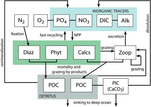
In this latest version, the general phytoplankton PFT is exactly replicated but given new parameter values to reflect key physiological characteristics of phytoplankton calcifiers, albeit biased towards Emiliania huxleyi. This new model version therefore contains “phytoplankton calcifiers,” “diazotrophs,” and “general phytoplankton.” The general phytoplankton PFT includes diatoms as well as all other autotrophic non-calcifying phytoplankton. Just as the general phytoplankton PFT cannot perfectly describe the physiology or ecology of any of the individual classifications of phytoplankton it represents, the calcifying PFT represents a group of phytoplankton with a common role in the carbonate cycle (calcification) and a few generalized shared physiological traits. In this new model, only calcifying phytoplankton and the zooplankton PFT produce CaCO₃. The CaCO₃ is calculated prognostically as a model tracer, and dissolution of phytoplankton calcifier and zooplankton export is now dependent on ambient carbonate concentration. The new model schematic is shown in Fig. 1.

Fig. 1 UVic ESCM biogeochemical model schematic. Arrows indicate the flux direction of nutrients.

In the following model description, notation will generally follow the symbols used in Keller et al. (2012), with additionally P standing for the general phytoplankton PFT, C standing for the phytoplankton calcifier PFT, and Z representing zooplankton when a distinction is necessary. Relevant model parameters are listed in Tables 1–4, with the Keller et al. (2012) model being referred to as NOCAL and this version being referred to as CAL. The model description here covers only the most relevant equations and equations that have changed in this newest version; please see Keller et al. (2012), Schmittner et al. (2005), and Schmittner et al. (2008) for a complete description of the other equations.

Table 1. Miscellaneous UVic ESCM biogeochemical model parameters. Temperature-dependent parameter values are given for 0°C.

Parameter	Symbol	Units	NOCAL	CAL
Diazotroph growth handicap		unitless	0.4	0.4
E-folding temperature		°C	15.65	15.65
Detrital remineralization rate		d^−1	0.055	0.055
Detrital sinking speed at surface		m d^−1	14.0	14.0
Ballast:Total detrital production ratio		unitless	N/A	0.05
Molar organic P:N ratio		unitless	0.0625	0.0625
Molar organic C:N ratio		unitless	6.625	6.625
Molar organic O:N ratio		unitless	10.0	10.0

Table 2. UVic ESCM CaCO₃ export-production parameters.

Parameter	Symbol	Units	NOCAL	CAL
CaCO3:POC production ratio		unitless	0.03	0.04
CaCO3 dissolution half-saturation constant	k	mmol C m^−3	N/A	100
CaCO3 sinking speed		m d^−1	N/A	35
Light attenuation by CaCO3		(m mmol m^−3)^−1	N/A	0.47

Table 3. UVic ESCM biogeochemical model phytoplankton production parameters. Temperature-dependent parameter values are given for 0°C.

Parameter	Symbol	Units	NOCAL	CAL
Maximum growth rate		d^−1	0.6	0.6
			N/A	0.52
Half-saturation constant N		mmol m^−3	0.7	0.7
			N/A	0.4
Half-saturation approximation constant Fe		nmol m^−3	0.1^a	0.1
			N/A	0.06
			0.1	0.12
Initial slope of P-I^b curve		(W m^−2)^−1 d^−1	0.1	0.1
			N/A	0.06
Light attenuation by phytoplankton		(m mmol m^−3)^−1	0.47	0.43
Phytoplankton mortality rate		d^−1	0.03	0.03
			N/A	0.03
			0.015	0.015
Microbial fast recycling		d^−1	0.015	0.015
			N/A	0.015

^aUVic ESCM value is tuned to an iron mask and is not the actual physiological iron limitation. See Keller et al. (2012) for a detailed discussion.

^bP−I is photosynthesis minus irradiance.

Table 4. UVic ESCM biogeochemical model zooplankton parameters. Temperature-dependent parameter values are given for 0°C.

Parameter	Symbol	Units	NOCAL	CAL
Maximum grazing rate		d^−1	0.4	0.4
Maximum grazing rate parameters		unitless	1.066	1.066
		°C^−1	1.0	1.0
Food preferences		unitless	0.30	0.225
			N/A	0.225
			0.30	0.225
			0.10	0.1
			0.30	0.225
Half-saturation constant		mmol m^−3	0.15	0.15
Growth efficiency constant		unitless	0.4	0.4
Assimilation efficiency		unitless	0.7	0.7
Mortality rate		d^−1	0.06	0.06

b Model Description

Tracer concentrations () vary according to:(3) with T including all transport terms (advection, diffusion, and convection) and representing all source and sink terms.

1 Phytoplankton

General phytoplankton and calcifying phytoplankton ( representing either) population source and sink terms are(4) where the growth rate (), mortality (), and fast recycling () terms are described below, and losses to zooplankton grazing () are described in Section 2b2. The diazotroph population sources and sinks follow(5)

As in Schmittner et al. (2005), the maximum possible growth rate of general phytoplankton and phytoplankton calcifiers () is a modified Eppley curve (Eppley, 1972) and is a function of seawater temperature (), an e-folding temperature parameter , and iron availability (). Parameter values are listed in Table 3. Phytoplankton calcifiers are assigned a lower maximum growth rate () than mixed phytoplankton, an assumption used previously by Le Quéré et al. (2005) but also justified by comparing measured growth rates for a selection of four coccolithophores by Buitenhuis, Pangerc, Franklin, Le Quéré, and Malin (2008) (0.3–1.0 d⁻¹ at 15°C) with the general range for phytoplankton by Eppley (1972) (a maximum rate of about 2.2 d⁻¹ at 15°C).(6) Iron limitation is calculated from the concentration of iron prescribed in interpolated monthly-mean fields using an iron half-saturation approximation constant () (Galbraith, Gnanadesikan, Dunne, & Hiscock, 2010; Keller et al., 2012). A prognostic iron cycle was recently implemented in the UVic ESCM (Nickelsen, Keller, & Oschlies, 2014), though it adds computational expense. However, accounting for iron limitation on growth rates by means of a limitation mask improves phytoplankton biogeography without additional computational cost (Keller et al., 2012). Calcifying and mixed phytoplankton are assigned different values that vary the degree of iron limitation and are tuned to produce the best possible PFT distributions, not actual iron affinities. Phytoplankton calcifiers are assigned a lower value than mixed phytoplankton to simulate the relatively low iron half-saturation constant for phytoplankton calcifiers recommended by Le Quéré et al. (2005):(7)

The maximum potential growth rate is then multiplied by a nutrient availability () for both nitrate (NO) and phosphate (PO) to calculate growth under nutrient limitation, where and are half-saturation constants:(8) (9)

These equations are applied to obtain maximum possible growth rates as a function of temperature and nutrients. As in Schmittner et al. (2005), the maximum possible growth rate under limited light availability () is calculated as:(10) where is the initial slope of the photosynthesis versus irradiance () curve. Phytoplankton calcifiers have a lower than diatoms, though it is similar to non-bloom-forming mixed phytoplankton (summarized in Le Quéré et al., 2005). Therefore, a lower value for phytoplankton calcifiers is used here. Additionally, light scattering by coccoliths is considered in calculating available irradiance at each depth level:(11) where PAR stands for the photosynthetically available radiation; , , , and are the light attenuation coefficients for water, all phytoplankton (calcifiers, diazotrophs, and general phytoplankton), CaCO₃, and ice, respectively; is the effective vertical coordinate; is the fractional sea-ice cover; and and are calculated sea-ice and snow cover thickness. Values for and come from Balch and Utgoff (2009).

The actual growth rate () of the general phytoplankton and calcifying phytoplankton PFTs is taken to be the minimum of the three growth functions described above:(12)

Diazotroph growth is not dependent on NO concentration and hence follows(13)

Two loss terms other than predation (described below) are considered. Mortality from old age or disease is parameterized using a linear mortality rate (). Temperature-dependent fast remineralization is a loss term used to account for the microbial loop and dissolved organic matter cycling and is parameterized using a temperature dependency multiplied by a constant ():(14)

2 Zooplankton

Zooplankton population () is calculated as the total available food (POC) scaled with a growth efficiency coefficient () minus mortality. In addition to old age and disease, zooplankton mortality also encompasses losses from higher trophic level predation and starvation.(15)

Zooplankton grazing () follows Keller et al. (2012). Relevant parameters are listed in Table 4. Grazing of each food source (mixed phytoplankton, calcifying phytoplankton, diazotrophs, zooplankton, and detritus) is calculated using a Holling Type-II function, in which a calculated maximum zooplankton grazing rate () is reduced by a scaling that is weighted by a food preference (, where stands for any of general phytoplankton, calcifying phytoplankton, diazotrophs, zooplankton, or total detritus), the total prey population, and a half-saturation constant for zooplankton ingestion ():(16)

Other formulations of grazing exist; see Anderson, Gentleman, and Sinha (2010) for a detailed comparison using two zooplankton size classes. Because the focus of this study is the implementation of a calcifying phytoplankton functional type, the grazing parameterization was not modified. The calculated maximum potential grazing rate is a function of a maximum potential grazing rate at 0°C (), temperature, and oxygen (sox stands for suboxic), where grazing activity is capped when temperatures exceed 20°C:(17)

Grazing is also reduced under hypoxic conditions ():(18) where O₂ is dissolved oxygen in micromol.

3 Detritus

Detritus sources and sinks now include contributions from phytoplankton calcifiers and are split into free and ballast pools using a fixed ratio (). Ballasted detritus is formed of the CaCO₃-protected portion of phytoplankton calcifier and zooplankton grazing and mortality. For simplicity, the same is used for both phytoplankton calcifiers and zooplankton. This protected portion does not interact with nutrient pools directly but instead transfers from the ballast to free detrital pool at the rate of CaCO₃ dissolution (; Eq. (33)):(19) (20) (21) where is the food assimilation efficiency, is a fixed production ratio of CaCO₃ and detritus, is a Redfield molar ratio, and is the detrital remineralization rate. As in Keller et al. (2012), detritus is exported from the surface with a sinking speed () that increases linearly (in per second units) with depth:(22) (23)

The initial surface sinking speeds of POC and CaCO₃ () are assigned different values to represent the denser structure of CaCO₃ relative to that of POC. Ballasted detritus sinks at the CaCO₃ speed, but once it enters the free pool it uses the detrital sinking speed and remineralization rate. Any detritus reaching the sediments is dissolved back into the water column.

4 Dissolved biogeochemical tracers

Ocean nutrient sources and sinks follow:(24) (25) where and are Redfield molar ratios, and is the Michaelis-Menten nitrate uptake rate. In suboxic (sox) water, oxygen consumption is replaced by the oxidation of nitrate(26) (27) and ocean surface dissolved oxygen exchanges with the atmosphere ().

The DIC and alkalinity tracer sources and sinks are now also a function of sources and sinks of prognostic CaCO₃ (Section 2b5):(28) (29)

5 Calcite production and export

The original model fixed CaCO₃ production to POC using a uniform ratio of CaCO₃ production to non-diazotrophic POC (detritus) production (). The CaCO₃ produced then contributed to DIC and alkalinity with a fixed remineralization profile exponentially dependent on depth. In our model, the general phytoplankton PFT no longer contributes to CaCO₃ but is instead replaced with the phytoplankton calcifier PFT. Different values for zooplankton and phytoplankton calcifiers can be assigned in case the ballast model is turned off, but a second ballasted detritus tracer would be required for this feature to be used with the ballast model. This second detritus tracer is not yet implemented, so the tuned model presented here includes ballast and a shared value for zooplankton and phytoplankton calcifiers. In earlier versions of the UVic ESCM, an value of 0.03 was used. In this version, it is increased to 0.04, which places it closer to (but still outside) the low end of the 0.05–0.25 range estimated by others and summarized by Fujii, Ikeda, and Yamanaka (2005). A CaCO₃:POC production ratio for E. huxleyi is summarized by Paasche (2001) to vary between 0.51 and 2.30, depending upon nutrient status and strain. A lower rain ratio for the model, therefore, indicates that the phytoplankton calcifier PFT cannot be considered to represent calcifiers exclusively, with other non-calcifying phytoplankton sharing the physiological traits also represented by the PFT. Likewise, calcification by the zooplankton PFT must be considered a global zooplankton average, with the zooplankton PFT representing all calcifying and non-calcifying zooplankton.

Production and dissolution of CaCO₃ are now a source and sink of a prognostic CaCO₃ tracer (Eq. (31)). Calcite held in living tissue is calculated separately as the net source–sink from phytoplankton calcifiers and zooplankton (Eqs (4) and (15)), converted to CaCO₃ units:(30) where is the Redfield ratio (Table 1).

New model tracer particulate CaCO₃ (in non-living form) follows the same general model structure as detritus, though the base units are millimoles of carbon per cubic metre rather than millimoles of nitrogen per cubic metre. One critical difference exists, which is that any CaCO₃ consumed by zooplankton is assumed to pass through the digestive system unaltered and is not assimilated into zooplankton growth. The source and sink terms for CaCO₃ include both phytoplankton calcifier and zooplankton sources from grazing and mortality, as well as losses from dissolution and sinking:(31)

The full equation of particulate CaCO₃ is thus:(32) with including all transport terms (advection, diffusion, and convection).

A CaCO₃ dissolution rate () that allows for supersaturated dissolution (Milliman et al., 1999) is calculated using a fixed dissolution rate parameter (k), following the calculation used in the Pelagic Interaction Scheme for Carbon and Ecosystem Studies (PISCES) model family (Aumont et al., 2003):(33) where is the deviance of the ambient seawater carbonate concentration from saturation () and any negative is set to zero.

Particulate CaCO₃ that reaches the sediments accumulates in an oxygen-only respiration model following Archer (1996b) that is unchanged from earlier versions of the UVic ESCM. During model spin-up, losses of alkalinity and carbon to the sediment model are exactly compensated for by a terrestrial weathering flux (diagnosed from the net sediment burial rate) that is applied as a flux of alkalinity and DIC to the ocean through river discharge. Once the model is in equilibrium either a constant or a prognostic terrestrial weathering flux can be used (Meissner et al., 2012).

The changes described in the above section improve the mechanistic realism of the UVic ESCM by explicitly including a phytoplankton functional type (phytoplankton calcifiers) that is both uniquely vulnerable to resource competition and uniquely responsible for CaCO₃ production and export. Representation of the CaCO₃ cycle in the UVic ESCM is additionally improved by including thermodynamic dissolution and detrital ballasting.

3 Model tuning

a Stabilizing Alkalinity

Model tracers, alkalinity and DIC are very sensitive to the prognostic CaCO₃ described in the previous section, which made model tuning a challenge. Stabilizing the model with realistic parameter values required multiple steps. After each step, conservation of global alkalinity and carbon was confirmed before proceeding. The original UVic ESCM ocean chemistry is in fairly good agreement with observations, so the initial goal was to tune the model as closely as possible to the original output. To do this, annual mean CaCO₃ dissolution at a pre-industrial equilibrium was diagnosed from the original model. The output file was then used as input to the new model (but, for structural reasons, without the ballast model turned on) to prescribe CaCO₃ dissolution. Production of CaCO₃ in the new model was not dramatically changed from the original model, but the possibility of greater dissolution than production in any given grid box meant a correction term was required to avoid negative CaCO₃ concentrations. The CaCO₃ tracer was, therefore, calculated from the ocean bottom to the surface in a reverse depth loop, and when the tracer was calculated as negative, a correction term was added to the concentration to set the tracer equal to zero. The correction term was then carried into the tracer calculation in the grid box above, which was likewise adjusted with a correction term if needed. At the surface, the integrated correction was added to the total CaCO₃ production to conserve carbon. In this way, the new model with a prognostic CaCO₃ tracer was able to reproduce the alkalinity and DIC fields of the original instant-export-production model.

b Adjusting Phytoplankton Production

The next step was to tune production as closely as possible to average global estimates and PFT distributions in the modern ocean (Table 5). Production parameters have been shown to be highly model dependent (Kriest & Oschlies, 2011). Parameters were adjusted under the constraints that mixed phytoplankton parameters be kept at original model parameter values and that phytoplankton calcifier growth rate, nitrogen and iron uptake, and values would all be lower than the mixed phytoplankton parameter values (Le Quéré et al., 2005). According to Scott, Kettle, and Merchant (2011), over 10% of model variance in primary production is attributable to four parameters: maximum growth rate (, in the high and mid-latitudes); the initial slope of the photosynthesis-irradiance curve (, at all latitudes); mortality (a more model-dependent variable having the largest impact at low latitudes, and here); and the carbon to chlorophyll ratio (at low latitudes, but not included in this model). Growth rate was by far the most sensitive of the production parameters in this model, with mortality and having less of an influence on biomass and biogeography. As has been shown previously (e.g., Cropp & Norbury, 2009), achieving multiple extant PFTs required careful model tuning. Nutrient half-saturation constants for nitrate and iron provided phytoplankton calcifiers a competitive advantage, whereas a lower growth rate and produced a disadvantage. The tuning of these parameters (, , , and ) required an iterative process to sufficiently “balance” the relative advantages with the relative disadvantages such that both general phytoplankton and calcifying phytoplankton populations remained extant and roughly realistically distributed in the surface ocean. As in other multiple-PFT models (e.g., Cropp & Norbury, 2009) similar growth rates for phytoplankton calcifiers and general phytoplankton were required to maintain both populations, but more variable nutrient uptake and grazing parameter values were possible.

Table 5. Globally integrated biological properties.

Property	NOCAL	CAL	Independent Estimate
Primary production (Pg C y^−1)	61.82	64.19	44–78^a
Export production at 130 m (Pg C y^−1)	7.77	7.09	5.73^b
POC flux at 2 km (Pg C y^−1)	0.26	0.36	0.43 ± 0.05^b
CaCO3 export at 130 m (Pg C y^−1)	0.94	0.83	1.1 ± 0.3^c
CaCO3 flux at 2 km (Pg C y^−1)	0.55	0.43	0.41 ± 0.05^b
CaCO3 dissolution (Pg C y^−1)	N/A	0.40	0.5 ± 0.2^d
CaCO3 sediment flux (Pg C y^−1)	0.48	0.42	0.21–0.27^e
Total phytoplankton (Pg C)	0.52	0.47	0.5–2.4^f
Phytoplankton calcifiers (Pg C)	N/A	0.15	0.001–0.03^g
Zooplankton (Pg C)	0.55	0.59	0.03–0.67^h

^aLow value from Carr et al. (2006), high value from Jin et al. (2006). Buitenhuis, Hashioka, and Le Quéré (2013b) recently used a model–data synthesis to constrain the value to 56 Pg C y⁻¹.

^bFrom Honjo et al. (2008).

^cFrom Lee (2001).

^dFrom Feely et al. (2004).

^e0.1–0.14 Pg C y⁻¹ in pelagic zones, 0.11–0.13 Pg C y⁻¹ in coastal zones, from Iglesias-Rodríguez et al. (2002).

^fTotal global autotrophic biomass from Buitenhuis et al. (2013a).

^gFrom Buitenhuis et al. (2013a).

^hCalcifying zooplankton only, from Buitenhuis et al. (2013a).

c Implementing Prognostic CaCO₃ Dissolution

With fixed CaCO₃ dissolution, tuned production, and stable alkalinity and DIC, the next step was to tune the CaCO₃ sinking rate. A sensitivity study across a range of and values was conducted to determine the combination that yielded the best fit to the original model CaCO₃ export (Table 5) and did not substantially alter ocean alkalinity distributions. After these parameter values were determined, the model was integrated for several thousand years to achieve an equilibrated state. The new model CaCO₃ dissolution scheme was run in parallel as a diagnostic only and tuned to approximate the original model dissolution. The new model CaCO₃ dissolution scheme replaced the original dissolution scheme after model equilibrium was achieved. The reverse-loop correction of CaCO₃ was not necessary after this step, so it was turned off and CaCO₃ was treated the same as any other tracer in the model.

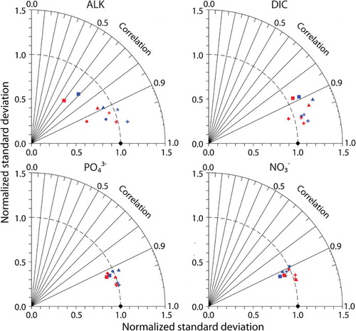
The CaCO₃ ballasting of detritus was the last component of the model to be turned on. Parameters , , , and were then re-evaluated to determine the optimal values. The model was tuned to reproduce (as best as possible) Global Data Analysis Project (GLODAP) and World Ocean Atlas (WOA) observations (Figs 2 and 3; Garcia et al., 2009; Key et al., 2004). The Taylor diagrams (Taylor, 2001) shown in Fig. 3 compare the correlation and standard deviation of model-simulated tracers normalized against the standard deviation of GLODAP and WOA observations. This section offers an example of how major structural modifications to existing models may not be possible without adopting an “engineering” approach of implementing model-stabilizing intermediate measures that are later removed.

Fig. 2 Averaged biogeochemical simulated tracers (CAL, solid red line; NOCAL, dashed blue line) compared with observations (black line). DIC and alkalinity observations are the standard GLODAP product (Key et al., 2004). Phosphate and nitrate observations are annual averages from the World Ocean Atlas (WOA; Garcia et al., 2009). Bottom row shows globally averaged model-data misfits.

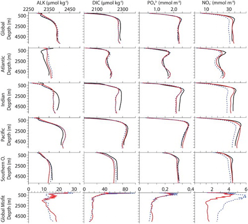
Fig. 3 Normalized Taylor diagrams of simulated tracers (CAL, red symbols; NOCAL, blue symbols) compared with observations (black circle). Observations used are as in Fig. 2. Ocean basins are denoted as global average (star), Atlantic (square), Indian (triangle), Pacific (plus), and Southern Ocean (diamond). The distance to the origin represents the normalized standard deviation. Normalized correlation with the observations is read from the azimuthal position. Perfect agreement with observations is a normalized standard deviation of 1 and a normalized correlation of 1.

d Alternative Grazing Parameterisations

Alternative grazing parameterizations such as prey switching (e.g., Fasham, Ducklow, & McKelvie, 1990; Prowe, Pahlow, Dutkiewicz, Follows, & Oschlies, 2012; Ryabchenko, Fasham, Kagan, & Popova, 1997) and the inclusion of kill-the-winner feeding (Vallina, Ward, Dutkiewicz, & Follows, 2014) have been proposed to address the common multi-PFT model problem of phytoplankton population instability encountered using the Holling Type-II grazing function. These alternatives produce a top-down control on biodiversity that can improve model agreement with phytoplankton diversity and bloom succession observations (Prowe et al., 2012) and reduce the competitive exclusion (Prowe et al., 2012; Vallina et al., 2014). Although these parameterizations might similarly improve UVic ESCM model performance, they have not been included in this model for a number of reasons. The primary objective of this study is to include prognostic CaCO₃ and a phytoplankton type resembling calcifiers and to compare these changes with the previous model. Simultaneously changing the grazing formulation would complicate the comparison and would, furthermore, require considerable additional experimentation to choose and tune the new formulation. Such an ambitious modification would be better suited to a separate study and will be seriously considered for inclusion in the model in the future. It is also important to remember that although prey switching does have a stabilizing effect, this does not necessarily mean that the assumptions behind it, or any grazing formulation for that matter, are correct (Anderson et al., 2010).

4 Model assessment

For the purpose of evaluation, the NOCAL and CAL versions of the model (from Keller et al., 2012, and as described here) were first brought to pre-industrial equilibrium using a fixed atmospheric CO₂ concentration of 283 ppm and integrated over ten thousand years. In each case the same physical parameters were used, and the sediment model was applied to both integrations (it was not used by Keller et al., 2012).

Model CAL biogeochemical tracers averaged globally and by ocean basin reveal generally improved performance with respect to NOCAL in reproducing GLODAP and WOA observations (Figs 2 and 3; Garcia et al., 2009; Key et al., 2004). This may be partly due to the application of a parameter set in NOCAL that was tuned by Keller et al. (2012) to a model that did not include sediments, whereas the parameter set in CAL is tuned to achieve the best fit including sediments. Both CAL and NOCAL perform well globally and in the Pacific and Southern oceans, with larger differences in the Indian and Atlantic basins. The fields show a clear improvement between CAL and NOCAL model versions whereas the fields are more mixed. Note that the objective was to improve the mechanistic realism of the model without sacrificing model performance with respect to the biogeochemistry, and overall this is achieved. Globally integrated biogeochemical properties for CAL and NOCAL (Table 5) reveal that although both model versions calculate global net primary production (NPP) within observational range, much of the production occurs in the eastern Pacific and Indian oceans (Figs 4h and 4i). High production in these regions is primarily from the general phytoplankton PFT in both CAL and NOCAL (Figs 4a and 4e), though phytoplankton calcifiers offer an important contribution in the CAL model (Fig. 4b). High production in the Indian basin can explain generally low surface nutrient, DIC, and alkalinity concentrations in this region (Figs 5 to 7). In the Atlantic, the model performs well with respect to observations of and DIC. As with earlier model versions (e.g., Eby et al., 2009), the most notable discrepancy between Atlantic observations and model results is in surface alkalinity concentrations (Fig 7), in which model alkalinity is too low in the northern hemisphere mid-latitudes and tropics. Surface DIC in the western Pacific Ocean is improved in the CAL version compared with earlier versions (not shown), though DIC in this region remains too low with respect to observations (Fig. 6) because of high model NPP.

Fig. 4 Depth-integrated annual average PFT biomass (g C m⁻²): (a) CAL general phytoplankton; (b) CAL phytoplankton calcifiers; (c) CAL diazotrophs; (d) CAL zooplankton; (e) NOCAL general phytoplankton; (f) NOCAL diazotrophs; (g) NOCAL zooplankton. Also shown is depth-integrated NPP (g C m⁻² d⁻¹) for (h) CAL and (i) NOCAL.

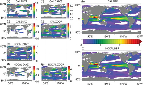
Fig. 5 Zonally averaged by ocean basin and surface distributions (CAL, left column; WOA observations, right column).

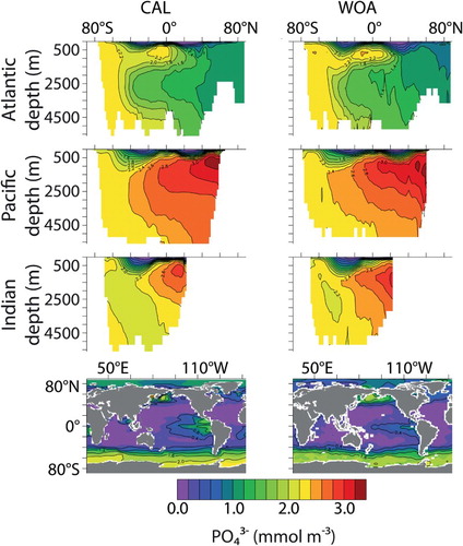
Fig. 6 Zonally averaged DIC by ocean basin and surface distributions (CAL, left column; GLODAP observations, right column).

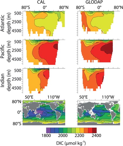
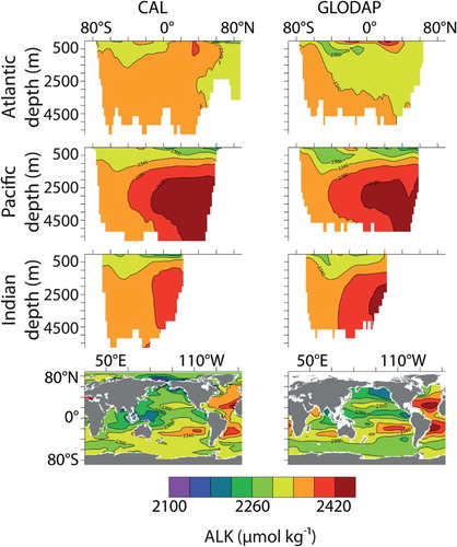
Fig. 7 Zonally averaged alkalinity by ocean basin and surface distributions (CAL, left column; GLODAP observations, right column).

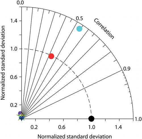
The concentration of CAL CaCO₃ peaks in latitudinal bands centred on 50°N, the equator, and 40°S (Fig 8). Limited data exist for this key model variable. Comparison with the Aqua Moderate Resolution Imaging Spectroradiometer (MODIS) standard CaCO₃ satellite product (NASA, 2013) reveals large differences between model-predicted and satellite-based concentrations, with the majority of CAL CaCO₃ occurring at low latitudes (because of high NPP) not represented in the satellite product. Lower CaCO₃ estimates by the model at high latitudes are the result of phytoplankton calcifiers being outcompeted by the faster-growing general phytoplankton PFT, as well as the model not simulating bloom dynamics. Satellite data must be used with caution because they have a seasonal bias, do not distinguish between living and dead CaCO₃ (Tyrrell & Merico, 2004), and can overestimate CaCO₃ by two to three times (Balch et al., 2011). Furthermore, Brown and Yoder (1994) estimate subpolar blooms captured by satellite might only represent 0.3% of the total global calcification, with the majority of coccoliths appearing in sediments having a source that is not detectable by satellites. In situ CaCO₃ and POC concentration data are more reliable but sparser. Model living and detached CaCO₃ and POC (detritus and PFT biomass) are used to compare simulated organic and inorganic carbon with in situ samples (Fig. 9). Regression of CAL concentrations with the data compilation of Lam, Doney, and Bishop (2011) show good agreement in simulated POC concentrations in the uppermost 1000 m. Simulated concentrations of living and detached CaCO₃ are underestimated with respect to Lam et al. (2011) for values indicative of blooms (greater than 0.5 mmol C m⁻³). Simulated CaCO₃ concentrations less than 0.2 mmol C m⁻³ are overestimated, which is consistent with higher simulated biomass in the low latitudes. A comparison of detached CaCO₃ concentration in CAL with the pre-industrial control concentration of the Coupled Model Intercomparison Project, Phase 5 (CMIP5) multi-model ensemble, normalized to the Lam et al. (2011) dataset shows CAL is within the range of CMIP5 models for which these data are available (Fig. 10).

Fig. 8 Zonally averaged CaCO₃ concentration by ocean basin (left and middle panels). Model CAL CaCO₃ concentration, including living CaCO₃ attached to phytoplankton calcifiers and zooplankton, in the surface grid box (to 50 m depth, top right panel). Bottom right is the standard CaCO₃ product from Aqua MODIS, accumulated over the entire mission (2002–2013; NASA, 2013).

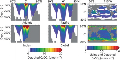
Fig. 9 Regression between modelled and observed CAL CaCO₃ concentration (left panel) and CAL POC concentration (right panel) from the ocean surface to 1000 m depth. Data are in situ measurements from Lam et al. (2011).

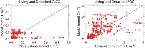
Fig. 10 Normalized Taylor diagram of model CaCO₃ concentrations compared with the Lam et al. (2011) dataset (black circle). Models are CAL (red circle), GFDL-ES2M (green star), MIROC-ESM (light blue circle), CNRM-CM5 (blue diamond), MPI-ESM-LR (yellow plus), and IPSL-CM5B-LR (purple circle). With the exception of CAL, the data for all models were obtained by mining the CMIP5 database (http://cmip-pcmdi.llnl.gov) using the following search terms: CMIP5/ocean biogeochem/pre-industrial control/annual output/calcite concentration.

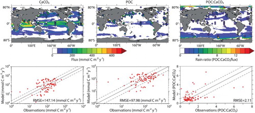
Annually averaged global CaCO₃ export fluxes (Table 5 and Fig. 11) are low compared with sediment trap data from Honjo, Manganini, Krishfield, and Francois (2008), though both CaCO₃ and POC fluxes in CAL agree better with observations than those in the NOCAL version (CaCO₃ root mean square error (RMSE) of 147.14 in CAL compared with 188.02 in NOCAL, POC RMSE of 97.98 in CAL compared with 100.65 in NOCAL). Improved fluxes are likely a result of the addition of the variable dissolution scheme, which calculates a global average dissolution rate of 0.40 Pg C per year (also low but within the range of error when compared with independent estimates, Table 5). Although application of a ballasting scheme was found to improve POC fluxes, the tuned ballasting parameter yields only a small ballasted POC pool that contributes only 2.6% of the POC reaching the sediments, compared with 80–83% estimated by Klaas and Archer (2002). Spatial biases in export fluxes follow those found in CaCO₃ concentration, with too much export in the low latitudes and too little poleward of 60° compared with Honjo et al. (2008). Sarmiento et al. (2002) and Dunne, Hales, and Toggweiler (2012) both concluded, from simple box models, that the major contribution of CaCO₃ to global export must come from low-latitude, non-bloom-forming phytoplankton calcifiers or zooplankton, so perhaps the CAL model is performing better than direct comparison with trap and satellite data suggest. Six percent of global total carbon export flux at 50 m depth is CaCO₃, compared with the Jin et al. (2006) estimate of 4% of the total carbon flux leaving the euphotic zone (75 m depth). Model CAL rain ratio follows the pattern calculated in Sarmiento et al. (2002) of a small POC:CaCO₃ export ratio in the low latitudes that increases poleward.

Fig. 11 Model average CaCO₃ (upper left panel) and POC (upper middle panel) export and average POC:CaCO₃ rain ratio (upper right panel) at 2 m depth overlaid by trap data from Honjo et al. (2008). Regressions between modelled and observed values can be seen in bottom panels.

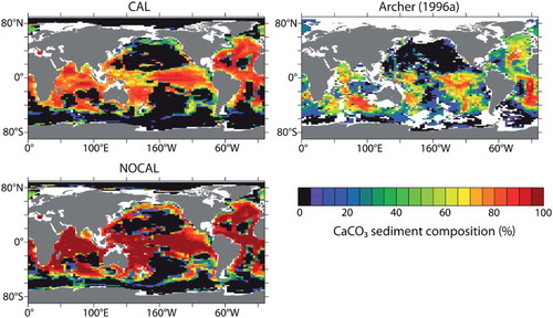
Simulated sediment composition in CAL varies only slightly from NOCAL, with overall lower contributions from CaCO₃ (Fig. 12). Although lower CaCO₃ concentrations represent an improvement compared with observational estimates (Archer, 1996a), concentrations are still too high because of the overproduction of phytoplankton calcifiers relative to total production. As in Dunne et al. (2012), the highest CaCO₃ fluxes to the sediments in the UVic ESCM correspond to regions with the highest CaCO₃ surface export production (not shown).

Fig. 12 Percentage CaCO₃ sediment composition. CAL is shown in upper left panel; NOCAL is shown in bottom left panel, and gridded sample data from Archer (1996a) is shown in top right panel.

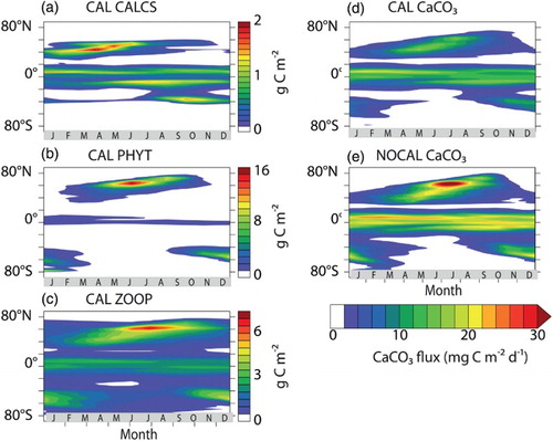
Unlike earlier versions of the UVic ESCM that used instant export and dissolution, CaCO₃ export now peaks about two months after phytoplankton calcifier biomass reaches seasonal maxima (Figs 13a and 13d). The CaCO₃ export is also now lower than in the NOCAL version (Table 5 and Fig. 13e). Model phytoplankton calcifiers bloom too early (March–May rather than June–July; O'Brien et al., 2013) in the northern latitudes. Zooplankton populations in the northern hemisphere high latitudes peaks about three months after phytoplankton calcifier biomass, with the seasonal progression being phytoplankton calcifiers first, then general phytoplankton, then zooplankton (Figs 13a to 13c). The model biomass succession is in contrast to the observed diatom to non-diatom progression (e.g., Joint, Pomroy, Savidge, & Boyd, 1993; Riebesell et al., 2007) though without explicit diatoms in the model it is expected that the model ecology could not replicate the behaviour of this keystone PFT. A previously noted correlation between Bering Sea Shelf E. huxleyi blooms and seasonal peaks in carbonate ion concentration (Merico, Tyrrell, & Cokacar, 2006) is also not seen in the CAL model because the proposed mechanism (precursor drawdown of DIC by a diatom bloom) is missing. Implementing an explicit dependence for phytoplankton calcifier growth on high would likely shift the phytoplankton calcifier biomass peak several months later in the season and move the general phytoplankton biomass peak forward, possibly improving model performance. Such a dependence might also improve CaCO₃ distributions by reducing the production and export in the low latitude upwelling zones. While increasing calcification correlates with increasing concentrations, no significant correlation between coccolith mass and chlorophyll or cell abundance is apparent in global sampling of surface water and sediment core samples (Beaufort et al., 2011). In the southern hemisphere, zooplankton seasonality is the primary driver of CaCO₃ fluxes because of the absence of a model phytoplankton calcifier population south of 40°S.

Fig. 13 Hovmöller diagrams of CAL depth-integrated PFT concentrations by latitude and month: (a) phytoplankton calcifiers, (b) general phytoplankton, (c) zooplankton. Also shown is CaCO₃ flux at 130 m depth by latitude and month for (d) CAL and (e) NOCAL.

Model phytoplankton calcifiers in CAL are reported as a molar concentration, whereas actual coccolithophores have cell biovolumes (in typical units of cubic micrometres) that are taxonomically variable (summarized in O'Brien et al., 2013). Hence, predicted phytoplankton calcifier concentrations in the CAL model are more indicative of the presence or absence of the PFT and cannot be expected to reasonably quantify abundance. Phytopankton calcifiers in CAL can be compared with the recent Marine Ecosystem Data (MAREDAT; Buitenhuis et al., 2013a; O'Brien et al., 2013) sample data synthesis. Because the CAL model does not resolve coastal processes, globally integrated total phytoplankton PFT concentrations (Table 5) are lower than the MAREDAT estimate. Phytoplankton calcifiers, however, are overrepresented by a factor of ten. This overestimate is primarily due to the low number of PFTs in the model, which requires that the phytoplankton calcifier PFT use parameter values (i.e., the growth rate factor) more similar to the general phytoplankton PFT than data support if it is to avoid extinction. The sparseness of the MAREDAT dataset limits conclusions to noting that the CAL model phytoplankton calcifiers have a far greater distribution than supported by in situ sampling and have the highest concentrations in low latitudes, in contrast to MAREDAT. The discrepancy mostly results from the overestimate of total production in this region coupled with the necessary overrepresentation of phytoplankton calcifiers to maintain an extant population. It may also be partly due to the likely sampling bias towards high-latitude blooms in the MAREDAT synthesis, with lower latitude open ocean regions having relatively few sample points (O'Brien et al., 2013). The CAL phytoplankton calcifier biomass maxima in the mid-latitudes (40°–60°N, 40°S) are generally consistent with observed high concentrations at 60°N and 20°–40°S (O'Brien et al., 2013) and high CaCO₃ export values at 40°N and 40°S calculated by Jin et al. (2006). Also consistent with MAREDAT is the lack of much seasonality in the Southern Ocean phytoplankton calcifier population.

Regional models with multiple PFTs (e.g., Litchman et al., 2006; Tyrrell & Taylor, 1996) or models using nutrient-restoring methods (e.g., Jin et al., 2006) are better able to represent coccolithophore abundances and community composition with data-based (rather than model-based) parameter values; Jin et al. (2006) estimate coccolithophores contribute only 2% of NPP, which is in better agreement with the MAREDAT relative abundance estimate for coccolithophores (Buitenhuis et al., 2013a). Models with fully prognostic PFTs applied in ocean general circulation models (OGCMs) have a more difficult time reproducing phytoplankton calcifier biogeography and proportionality. Coccolithophores in NASA's ocean biogeochemical model (NOBM; five PFTs) (Gregg et al., 2003; Gregg & Casey, 2007) show an overall positive correlation with in situ data, though fail to appear in the North Pacific and Antarctic regions. As with the CAL model, coccolithophores in NOBM are overrepresented in the equatorial Pacific Ocean (Gregg & Casey, 2007). Though the NOBM coccolithophores contribute more to global NPP (17%) than the Jin et al. (2006) estimate, this is still much lower than the contribution of CAL model phytoplankton calcifiers to total NPP of 44%. The biogeochemical Plankton Types Ocean Model, version 5.2 (PlankTOM5.2; five PFTs) applied to two different OGCMs cannot reproduce high-latitude phytoplankton calcifier populations, and mixed phytoplankton and phytoplankton calcifiers do not easily co-exist (Sinha, Buitenhuis, Le Quéré, & Anderson, 2010). Also apparent in the PlankTOM5.2 application in the Nucleus for European Modelling of the Ocean (NEMO) model is an overrepresentation of the phytoplankton calcifier population in the Indian and western Pacific basins (Sinha et al., 2010), which is a problem shared by this model.

Aside from phytoplankton calcifiers, PFT relative concentrations are otherwise in agreement with Buitenhuis et al. (2013a), with diazotrophs having the lowest concentration, followed by general phytoplankton. Diazotroph concentration is substantially lower than the general phytoplankton PFT and is able to remain extant because of its critical advantage of not being nitrogen limited. In CAL, as found by Buitenhuis et al. (2013a), zooplankton concentrations are higher than total phytoplankton concentrations.

Overall the CAL model advances UVic ESCM biogeochemistry by improving the mechanistic realism without sacrificing model performance with respect to nutrient and carbon distributions. As with any model, however, this one is not without caveats regarding its application. Collapsing complex and poorly understood natural biogeochemical cycles into a rigid artificial model structure introduces uncertainty into the parameter space of the constructed equations. The degree of underdetermination of the model equations is sufficiently large that a priori assumptions and optimization methods have been shown to influence results, with “optimal” parameter values comprising a broad range, each performing equally well with respect to independent data (Ward, Friedrichs, Anderson, & Oschlies, 2010). It is important to note that although this model has been tuned manually to reduce the model–data error in global state variables, it cannot be considered optimized (Kriest, Khatiwala, & Oschlies, 2010). Furthermore, nutrients, to a degree, and PFT distributions are especially sensitive to model structure and parameter choice (Anderson et al., 2010; Manizza, Buitenhuis, & Le Quéré, 2010; Sailley et al., 2013), as well as physical biases in any given ocean model (Doney et al., 2004; Najjar et al., 2007; Sinha et al., 2010). Similarly, models can perform comparatively well for very different structural reasons (Hashioka et al., 2013). It is, therefore, often difficult to determine whether the model is producing the right answer for the wrong reason (e.g., Friedrichs et al., 2007; Sinha et al., 2010). More specifically, biological parameter choice for the calcifying PFT is biased towards E. huxleyi, which necessarily biases model results. One must, therefore, be careful to interpret model results appropriately, given these limitations.

5 Conclusions

Calcifying phytoplankton and zooplankton are key components of the ocean carbon cycle and thus their representation in coupled climate models is important for understanding systemic response to change. This model is a unique attempt to include phytoplankton calcifiers as an explicit PFT alongside a general phytoplankton and diazotroph PFT in an intermediate complexity model and to make the phytoplankton calcifiers and zooplankton responsible for CaCO₃ production and prognostic export, as well as detrital ballasting. The UVic ESCM now fills a niche in Earth system modelling that was previously unoccupied in that it is relatively inexpensive to run, yet resolves the complete Earth system carbon cycle including prognostic CaCO₃ and a separate phytoplankton calcifier PFT. Because the UVic ESCM includes ocean sediments and calcite compensation it is now a model that is particularly well suited to reducing the uncertainty of the fate of emissions over the long term. It is now also well suited to testing the parameter space of feedbacks between the carbonate and carbon cycles and the climate system as transient simulations. The modifications maintain the UVic ESCM's performance with respect to nutrient distributions and carbon fluxes and make the model mechanistically more realistic. Primary production, export production, POC and CaCO₃ fluxes at various depths all fall within independent estimates. Though the model is able to reasonably reproduce observed patterns of mid-latitude maximum phytoplankton calcifier concentrations, it also shares biases common to other phytoplankton calcifier PFT models coupled to OGCMs: calcifiers are overrepresented in total biomass and in low latitudes, and underrepresented in high latitudes compared with satellite and sample data (Gregg & Casey, 2007; Sinha et al., 2010; Vogt et al., 2013). In the CAL model, failure to resolve coastal processes results in NPP, CaCO₃, and POC export-production fluxes that are necessarily too high in the low latitudes in order to match global estimates. With possibly 48% of total global POC flux occurring in water depths less than 50 m (Dunne, Sarmiento, & Gnanadesikan, 2007), lacking any sort of parameterization for these regions imposes a significant bias to the model. In other phytoplankton calcifier multi-PFT models, exact regions of bias are model dependent and attributable to physical and ecosystem differences, but the systematic overrepresentation of phytoplankton calcifiers in low latitudes may have some physical justification. Previous studies have shown global export budgets require high CaCO₃ export in this region (Sarmiento et al., 2002), and high latitude bloom CaCO₃ is underrepresented in sediments (Brown & Yoder, 1994). Vogt et al. (2013) noted the similarity of phytoplankton calcifier model biogeography to observed picophytoplankton biogeography, so inclusion of additional picophytoplankton PFTs might improve phytoplankton calcifiers in models.

The UVic ESCM is now approaching a level of carbonate–carbon cycle complexity in which recent hypotheses regarding internally driven feedbacks in glacial–interglacial atmospheric CO₂ concentration changes can be tested in an Earth system model. Reduction of the Si:N export ratio in the Southern Ocean during glaciation leading to the expansion of diatoms at the expense of coccolithophores (Matsumoto, Sarmiento, & Brzezinski, 2002) can be tested using the prognostic iron cycle of Nickelsen et al. (2014) once diatoms and silicate are implemented (currently underway). Increased calcifier concentration with increased ocean alkalinity driving sawtooth-shaped global CO₂ time series (Omta, van Voorn, Rickaby, & Follows, 2013) can be tested with the implementation of increased calcifier growth or advantage with increasing carbonate saturation state. The role of temperature-enhanced phytoplankton growth (Fowler, Rickaby, & Wolff, 2013) in glacial–interglacial transitions can also be tested.

This exercise reiterates the difficulty of simulating realistic CaCO₃ distributions because production and export depend on many physical, physiological, and ecological factors. There are five potential improvements to the CAL model that have not yet been addressed. Simulated phytoplankton calcifiers are wholly dependent on relative competitive advantage and can easily become extinct or cause the general phytoplankton PFT to become extinct with only small adjustments to production parameter values, especially the growth rate. Because their niche is so poorly defined with respect to the general phytoplankton PFT, additional PFTs (particularly diatoms) are expected to improve their population biogeography, stability, and seasonal behaviour and may allow phytoplankton calcifier parameter values to become less model- and more data-dependent (although this assumption has not been tested). Secondly, the ballast model does not include a parameterization for particle aggregation, which would increase the fraction of ballasted POC ending up in the sediments. Thirdly, static stoichiometric ratios in the model ignore their dependence on remineralization processes (Schneider, Schlitzer, Fischer, & Nothig, 2003), carbonate chemistry (Riebesell et al., 2007), biogeography (Weber & Deutsch, 2010), and taxonomy (Arrigo et al., 1999). Including a parameterization of flexible stoichiometric ratios would have a significant influence on the ecology (Flynn, 2010), nutrient distributions, and carbon uptake (Kortzinger, Koeve, Kahler, & Mintrop, 2001; Schneider et al., 2004). In a similar vein, experimentation with the parameterization of zooplankton (numbers of PFTs with variable grazing preferences, prey-switching, assimilation of consumed CaCO₃, a variable rain ratio, unique CaCO₃ dissolution parameters, etc.) would also likely produce insight into model sensitivity to zooplankton assumptions. Lastly, the model does not account for decreasing calcification with increasing CO₂ concentration (Riebesell et al., 2000), which would doubtless affect simulated tracer distributions and biogeography. Sustained declines in calcification are questionable (Lohbeck, Riebesell, & Reusch, 2012) and were therefore omitted. Furthermore, using a single dissolution parameterization for zooplankton and phytoplankton calcifier CaCO₃ ignores the likely significant contribution of aragonite dissolution to global alkalinity (Gangstø et al., 2008). These last two were considered for inclusion in this model, but the current code structure is not amenable to flexible or multiple rain ratios and will require a significant restructuring should these changes be implemented in the future.

Code availability

Model code can be obtained from the first author on request.

Acknowledgements

This work was supported by an award under the Merit Allocation Scheme on the National Computational Infrastructure facility at the Australia National University. KJM is grateful for support under the Australian Research Council's Future Fellowship programme (FT100100443). KFK is grateful for support from the University of New South Wales through a University International Postgraduate Award, and the ARC Centre of Excellence for Climate Science. The authors thank Laurie Menviel for her helpful comments on versions of the manuscript. The authors furthermore acknowledge the World Climate Research Programme's Working Group on Coupled Modelling, which is responsible for CMIP and thank the climate modelling groups cited in the manuscript for producing and making available their model output.

Disclosure statement

No potential conflict of interest was reported by the authors.

References

- Anderson, T. R., Gentleman, W. C., & Sinha, B. (2010). Influence of grazing formulations on the emergent properties of a complex ecosystem model in a global ocean general circulation model. Progress in Oceanography, 87(1–4, SI), 201–213. doi: 10.1016/j.pocean.2010.06.003
- Archer, D. (1996a). An atlas of the distribution of calcium carbonate in sediments of the deep sea. Global Biogeochemical Cycles, 10(1), 159–174. doi: 10.1029/95GB03016
- Archer, D. (1996b). A data-driven model of the global calcite lysocline. Global Biogeochemical Cycles, 10(3), 511–526. doi: 10.1029/96GB01521
- Armstrong, R., Lee, C., Hedges, J., Honjo, S., & Wakeham, S. (2002). A new, mechanistic model for organic carbon fluxes in the ocean based on the quantitative association of POC with ballast minerals. Deep-Sea Research Part II: Topical Studies in Oceanography, 49(1–3), 219–236. doi: 10.1016/S0967-0645(01)00101-1
- Arrigo, K., Robinson, D., Worthen, D., Dunbar, R., DiTullio, G., VanWoert, M., & Lizotte, M. (1999). Phytoplankton community structure and the drawdown of nutrients and CO2 in the Southern Ocean. Science, 283(5400), 365–367. doi: 10.1126/science.283.5400.365
- Aumont, O., & Bopp, L. (2006). Globalizing results from ocean in situ iron fertilization studies. Global Biogeochemical Cycles, 20(2). doi:10.1029/2005GB002591
- Aumont, O., Maier-Reimer, E., Blain, S., & Monfray, P. (2003). An ecosystem model of the global ocean including Fe, Si, P colimitations. Global Biogeochemical Cycles, 17(2). doi:101029/2001GB001745
- Balch, W. M., & Utgoff, P. E. (2009). Potential interactions among ocean acidification, coccolithophores, and the optical properties of seawater. Oceanography, 22(4, SI), 146–159. doi: 10.5670/oceanog.2009.104
- Balch, W. M., Drapeau, D. T., Bowler, B. C., Lyczskowski, E., Booth, E. S., & Alley, D. (2011). The contribution of coccolithophores to the optical and inorganic carbon budgets during the Southern Ocean gas exchange experiment: New evidence in support of the “Great Calcite Belt” hypothesis. Journal of Geophysical Research-Oceans, 116. doi: 10.1029/2011JC006941
- Beaufort, L., Probert, I., de Garidel-Thoron, T., Bendif, E. M., Ruiz-Pino, D., Metzl, N., … de Vargas, C. (2011). Sensitivity of coccolithophores to carbonate chemistry and ocean acidification. Nature, 476(7358), 80–83. doi: 10.1038/nature10295
- Brown, C., & Yoder, J. (1994). Coccolithophorid blooms in the global ocean. Journal of Geophysical Research-Oceans, 99(C4), 7467–7482. doi: 10.1029/93JC02156
- Buitenhuis, E. T., Hashioka, T., & Le Quéré, C. (2013b). Combined constraints on global ocean primary production using observations and models. Global Biogeochemical Cycles, 27(3), 847–858. doi: 10.1002/gbc.20074
- Buitenhuis, E. T., Pangerc, T., Franklin, D. J., Le Quéré, C., & Malin, G. (2008). Growth rates of six coccolithophorid strains as a function of temperature. Limnology Oceanography, 53, 1181–1185. doi: 10.4319/lo.2008.53.3.1181
- Buitenhuis, E. T., Vogt, M., Moriarty, R., Bednarsek, N., Doney, S. C., Leblanc, K., … Swan, C. (2013a). MAREDAT: Towards a world atlas of MARine Ecosystem DATa. Earth System Science Data, 5(2), 227–239. doi: 10.5194/essd-5-227-2013
- Carr, M.-E., Friedrichs, M. A. M., Schmeltz, M., Aita, M. N., Antoine, D., Arrigo, K. R., … Yamanaka, Y. (2006). A comparison of global estimates of marine primary production from ocean color. Deep-Sea Research Part II: Topical Studies in Oceanography, 53(5–7), 741–770. doi: 10.1016/j.dsr2.2006.01.028
- Cropp, R., & Norbury, J. (2009). Parameterizing plankton functional type models: Insights from a dynamical systems perspective. Journal of Plankton Research, 31(9), 939–963. doi: 10.1093/plankt/fbp042
- Doney, S., Lindsay, K., Caldeira, K., Campin, J., Drange, H., Dutay, J., … Yool, A. (2004). Evaluating global ocean carbon models: The importance of realistic physics. Global Biogeochemical Cycles, 18(3). doi:10.1029/2003GB002150
- Dunne, J. P., Hales, B., & Toggweiler, J. R. (2012). Global calcite cycling constrained by sediment preservation controls. Global Biogeochemical Cycles, 26(3). doi:10.1175/JCLI-0-11-00560.1
- Dunne, J. P., Sarmiento, J. L., & Gnanadesikan, A. (2007). A synthesis of global particle export from the surface ocean and cycling through the ocean interior and on the seafloor. Global Biogeochemical Cycles, 21(4). doi:10.1029/2006GB002907
- Dutay, J.-C., Bullister, J., Doney, S., Orr, J., Najjar, R., Caldeira, K., … Yool, A. (2002). Evaluation of ocean model ventilation with CFC-11: Comparison of 13 global ocean models. Ocean Modelling, 4(2), 89–120. doi: 10.1016/S1463-5003(01)00013-0
- Eby, M., Zickfeld, K., Montenegro, A., Archer, D., Meissner, K. J., & Weaver, A. J. (2009). Lifetime of anthropogenic climate change: Millennial time scales of potential CO2 and surface temperature perturbations. Journal of Climate, 22(10), 2501–2511. doi: 10.1175/2008JCLI2554.1
- Eppley, R. (1972). Temperature and phytoplankton growth in the sea. Fishery Bulletin, 70, 1063–1085.
- Fabry, V. (1989). Aragonite production by pteropod mollusks in the sub-arctic Pacific. Deep-Sea Research Part A. Oceanographic Research Papers, 36(11), 1735–1751. doi: 10.1016/0198-0149(89)90069-1
- Fasham, M., Ducklow, H., & McKelvie, S. (1990). A nitrogen-based model of plankton dynamics in the oceanic mixed layer. Journal of Marine Research, 48(3), 591–639. doi: 10.1357/002224090784984678
- Feely, R. A., Sabine, C. L., Lee, K., Berelson, W., Kleypays, J., Fabry, V. J., & Millero, F. (2004). Impact of anthropogenic CO2 on the CaCO3 system in the oceans. Science, 305(5682), 362–366. doi: 10.1126/science.1097329
- Flynn, K. J. (2010). Ecological modelling in a sea of variable stoichiometry: Dysfunctionality and the legacy of Redfield and Monod. Progress in Oceanography, 84, 52–65. doi: 10.1016/j.pocean.2009.09.006
- Fowler, A., Rickaby, R., & Wolff, E. (2013). Exploration of a simple model for ice ages. GEM - International Journal on Geomathematics, 4(2), 227–297. doi: 10.1007/s13137-012-0040-7
- Friedrichs, M. A. M., Dusenberry, J. A., Anderson, L. A., Armstrong, R. A., Chai, F., Christian, J. R., … Wiggert, J. D. (2007). Assessment of skill and portability in regional marine biogeochemical models: Role of multiple planktonic groups. Journal of Geophysical Research-Oceans, 112(C8). doi:10.1029/2006JC003852
- Fujii, M., Ikeda, M., & Yamanaka, Y. (2005). Roles of biogeochemical processes in the oceanic carbon cycle described with a simple coupled physical-biogeochemical model. Journal of Oceanography, 61, 803–815. doi: 10.1007/s10872-006-0001-6
- Fyke, J. G., & Weaver, A. J. (2006). The effect of potential future climate change on the marine methane hydrate stability zone. Journal of Climate, 19(22), 5903–5917. doi: 10.1175/JCLI3894.1
- Galbraith, E. D., Gnanadesikan, A., Dunne, J. P., & Hiscock, M. R. (2010). Regional impacts of iron-light colimitation in a global biogeochemical model. Biogeosciences, 7(3), 1043–1064. doi: 10.5194/bg-7-1043-2010
- Gangstø, R., Gehlen, M., Schneider, B., Bopp, L., Aumont, O., & Joos, F. (2008). Modeling the marine aragonite cycle: Changes under rising carbon dioxide and its role in shallow water CaCO3 dissolution. Biogeosciences, 5(4), 1057–1072. doi: 10.5194/bg-5-1057-2008
- Garcia, H. E., Locarnini, R., Boyer, T., Antonov, J., Zweng, M., Baranova, O., & Johnson, D. (2009). World Ocean Atlas 2009: Nutrients (phosphate, nitrate, silicate) (Vol. 4) (No. NOAA Atlas NESDIS 71). Washington, DC: U.S. Government Printing Office.
- Gehlen, M., Gangstø, R., Schneider, B., Bopp, L., Aumont, O., & Ethe, C. (2007). The fate of pelagic CaCO3 production in a high CO2 ocean: A model study. Biogeosciences, 4(4), 505–519. doi: 10.5194/bg-4-505-2007
- Gregg, W. W., & Casey, N. W. (2007). Modeling coccolithophores in the global oceans. Deep-Sea Research Part II: Topical Studies in Oceanography, 54(5–7), 447–477. doi: 10.1016/j.dsr2.2006.12.007
- Gregg, W., Ginoux, P., Schopf, P., & Casey, N. (2003). Phytoplankton and iron: Validation of a global three-dimensional ocean biogeochemical model. Deep-Sea Research Part II: Topical Studies in Oceanography, 50(22–26), 3143–3169. doi: 10.1016/j.dsr2.2003.07.013
- Hashioka, T., Vogt, M., Yamanaka, Y., Le Quéré, C., Buitenhuis, E. T., Aita, M. N., … Doney, S. C. (2013). Phytoplankton competition during the spring bloom in four plankton functional type models. Biogeosciences, 10(11), 6833–6850. doi: 10.5194/bg-10-6833-2013
- Heinze, C. (2004). Simulating oceanic CaCO3 export production in the greenhouse. Geophysical Research Letters, 31(16). doi:10.1029/2004GL020613
- Hofmann, M., & Schellnhuber, H.-J. (2009). Oceanic acidification affects marine carbon pump and triggers extended marine oxygen holes. Proceedings of the National Academy of Sciences of the United States of America, 106(9), 3017–3022. doi: 10.1073/pnas.0813384106
- Honjo, S., Manganini, S. J., Krishfield, R. A., & Francois, R. (2008). Particulate organic carbon fluxes to the ocean interior and factors controlling the biological pump: A synthesis of global sediment trap programs since 1983. Progress in Oceanography, 76(3), 217–285. doi: 10.1016/j.pocean.2007.11.003
- Hood, R. R., Laws, E. A., Armstrong, R. A., Bates, N. R., Brown, C. W., Carlson, C. A., … Wiggert, J. D. (2006). Pelagic functional group modeling: Progress, challenges and prospects. Deep-Sea Research Part II: Topical Studies in Oceanography, 53(5–7), 459–512. doi: 10.1016/j.dsr2.2006.01.025
- Iglesias-Rodrlguez, M. D., Armstrong, R., Feely, R., Hood, R., Kleypas, J., Milliman, J. D., … Sarmiento, J. (2002). Progress made in study of ocean's calcium carbonate budget. EOS, Transactions American Geophysical Union, 83(34), 365–375. doi: 10.1029/2002EO000267
- Jin, X., Gruber, N., Dunne, J. P., Sarmiento, J. L., & Armstrong, R. A. (2006). Diagnosing the contribution of phytoplankton functional groups to the production and export of particulate organic carbon, CaCO3, and opal from global nutrient and alkalinity distributions. Global Biogeochemical Cycles, 20(2). GB2015. doi:10.1029/2005GB002532
- Joint, I., Pomroy, A., Savidge, G., & Boyd, P. (1993). Size-fractionated primary productivity in the northeast Atlantic in May-July 1989. Deep-Sea Research Part II: Topical Studies in Oceanography, 40(1–2), 423–440. doi: 10.1016/0967-0645(93)90025-I
- Keller, D. P., Oschlies, A., & Eby, M. (2012). A new marine ecosystem model for the University of Victoria Earth System Climate Model. Geoscientific Model Development, 5(5), 1195–1220. doi: 10.5194/gmd-5-1195-2012
- Key, R., Kozyr, A., Sabine, C., Lee, K., Wanninkhof, R., Bullister, J., … Mordy, C. (2004). A global ocean carbon climatology: Results from GLODAP. Global Biogeochemical Cycles, 18. doi:10.1029/2004GB002247
- Klaas, C., & Archer, D. (2002). Association of sinking organic matter with various types of mineral ballast in the deep sea: Implications for the rain ratio. Global Biogeochemical Cycles, 16(4). doi:10.1029/2001GB001765
- Kortzinger, A., Koeve, W., Kahler, P., & Mintrop, L. (2001). C:N ratios in the mixed layer during the productive season in the northeast Atlantic ocean. Deep-Sea Research Part I: Oceanographic Research Papers, 48(3), 661–688. doi: 10.1016/S0967-0637(00)00051-0
- Kriest, I., & Oschlies, A. (2011). Numerical effects on organic-matter sedimentation and remineralization in biogeochemical ocean models. Ocean Modelling, 39(34), 275–283. doi: 10.1016/j.ocemod.2011.05.001
- Kriest, I., Khatiwala, S., & Oschlies, A. (2010). Towards an assessment of simple global marine biogeochemical models of different complexity. Progress in Oceanography, 86(3–4), 337–360. doi: 10.1016/j.pocean.2010.05.002
- Lam, P. J., Doney, S. C., & Bishop, J. K. B. (2011). The dynamic ocean biological pump: Insights from a global compilation of particulate organic carbon, CaCO3, and opal concentration profiles from the mesopelagic. Global Biogeochemical Cycles, 25. doi:10.1029/2010GB003868
- Le Quéré, C., Harrison, S., Prentice, I., Buitenhuis, E., Aumont, O., Bopp, L., … Wolf-Gladrow, D. (2005). Ecosystem dynamics based on plankton functional types for global ocean biogeochemistry models. Global Change Biology, 11(11), 2016–2040.
- Lee, K. (2001). Global net community production estimated from the annual cycle of surface water total dissolved inorganic carbon. Limnology and Oceanography, 46(6), 1287–1297. doi: 10.4319/lo.2001.46.6.1287
- Litchman, E., Klausmeier, C. A., Miller, J. R., Schofield, O. M., & Falkowski, P. G. (2006). Multinutrient, multi-group model of present and future oceanic phytoplankton communities. Biogeosciences, 3(4), 585–606. doi: 10.5194/bg-3-585-2006
- Lohbeck, K. T., Riebesell, U., & Reusch, T. B. H. (2012). Adaptive evolution of a key phytoplankton species to ocean acidification. Nature Geoscience, 5(5), 346–351. doi: 10.1038/ngeo1441
- Manizza, M., Buitenhuis, E. T., & Le Quéré, C. (2010). Sensitivity of global ocean biogeochemical dynamics to ecosystem structure in a future climate. Geophysical Research Letters, 37. doi: 10.1029/2010GL043360
- Matsumoto, K., Sarmiento, J., & Brzezinski, M. (2002). Silicic acid leakage from the Southern Ocean: A possible explanation for glacial atmospheric pCO2. Global Biogeochemical Cycles, 16(3). doi:10.1029/2001GB001442
- Matthews, H., Weaver, A., & Meissner, K. (2005). Terrestrial carbon cycle dynamics under recent and future climate change. Journal of Climate, 18(10), 1609–1628. doi: 10.1175/JCLI3359.1
- Matthews, H., Weaver, A., Eby, M., & Meissner, K. (2003). Radiative forcing of climate by historical land cover change. Geophysical Research Letters, 30(2). doi:10.1029/2002GL016098
- Meissner, K. J. (2007). Younger Dryas: A data to model comparison to constrain the strength of the overturning circulation. Geophysical Research Letters, 34(21). doi:10.1029/2007GL031304
- Meissner, K. J., Eby, M., Weaver, A. J., & Saenko, O. A. (2008). CO2 threshold for millennial-scale oscillations in the climate system: Implications for global warming scenarios. Climate Dynamics, 30(2–3), 161–174. doi: 10.1007/s00382-007-0279-0
- Meissner, K. J., McNeil, B. I., Eby, M., & Wiebe, E. C. (2012). The importance of the terrestrial weathering feedback for multimillennial coral reef habitat recovery. Global Biogeochemical Cycles, 26. doi:10.1029/2011GB004098
- Meissner, K., Weaver, A., Matthews, H., & Cox, P. (2003). The role of land surface dynamics in glacial inception: A study with the UVic Earth System Model. Climate Dynamics, 21(7–8), 515–537. doi: 10.1007/s00382-003-0352-2
- Merico, A., Tyrrell, T., & Cokacar, T. (2006). Is there any relationship between phytoplankton seasonal dynamics and the carbonate system? Journal of Marine Systems, 59(1–2), 120–142. doi: 10.1016/j.jmarsys.2005.11.004
- Milliman, J. (1993). Production and accumulation of calcium-carbonate in the ocean - budget of a nonsteady state. Global Biogeochemical Cycles, 7(4), 927–957. doi: 10.1029/93GB02524
- Milliman, J., Troy, P., Balch, W., Adams, A., Li, Y., & Mackenzie, F. (1999). Biologically mediated dissolution of calcium carbonate above the chemical lysocline?. Deep-Sea Research Part I: Oceanographic Research Papers, 46(10), 1653–1669. doi: 10.1016/S0967-0637(99)00034-5
- Moore, J., Doney, S., Kleypas, J., Glover, D., & Fung, I. (2002). An intermediate complexity marine ecosystem model for the global domain. Deep-Sea Research Part II: Topical Studies in Oceanography, 49(1–3), 403–462. doi: 10.1016/S0967-0645(01)00108-4
- Mysak, L., Wright, K., Sedlacek, J., & Eby, M. (2005). Simulation of sea ice and ocean variability in the Arctic during 1955–2002 with an intermediate complexity model. Atmosphere-Ocean, 43(1), 101–118. doi: 10.3137/ao.430106
- Najjar, R. G., Jin, X., Louanchi, F., Aumont, O., Caldeira, K., Doney, S. C., … Yool, A. (2007). Impact of circulation on export production, dissolved organic matter, and dissolved oxygen in the ocean: Results from phase II of the Ocean Carbon-cycle Model Intercomparison Project (OCMIP-2). Global Biogeochemical Cycles, 21(3). doi:10.1029/2006GB00285
- NASA (National Aeronautics and Space Administration). (2013). MODIS PIC data product [Data] (Tech. Rep.). Greenbelt, MD, USA: Goddard Space Flight Center, Distributed Active Archive Center. Retrieved from http://oceancolor.gsfc.nasa.gov/cms/citations
- Nickelsen, L., Keller, D. P., & Oschlies, A. (2014). A dynamic marine iron cycle module coupled to the University of Victoria Earth System Model: The Kiel Marine Biogeochemical Model 2 (KMBM2) for UVic 2.9. Geoscientific Model Development Discussions, 7(6), 8505–8563. doi: 10.5194/gmdd-7-8505-2014
- Nof, D., Van Gorder, S., & de Boer, A. (2007). Does the Atlantic meridional overturning cell really have more than one stable steady state? Deep-Sea Research Part I: Oceanographic Research Papers, 54(11), 2005–2021. doi: 10.1016/j.dsr.2007.08.006
- O'Brien, C. J., Peloquin, J. A., Vogt, M., Heinle, M., Gruber, N., Ajani, P., … Widdicombe, C. (2013). Global marine plankton functional type biomass distributions: Coccolithophores. Earth System Science Data, 5(2), 259–276. doi: 10.5194/essd-5-259-2013
- Omta, A. W., van Voorn, G. A. K., Rickaby, R. E. M., & Follows, M. J. (2013). On the potential role of marine calcifiers in glacial-interglacial dynamics. Global Biogeochemical Cycles, 27(3), 692–704. doi: 10.1002/gbc.20060
- Oschlies, A., Schulz, K. G., Riebesell, U., & Schmittner, A. (2008). Simulated 21st century's increase in oceanic suboxia by CO2-enhanced biotic carbon export. Global Biogeochemical Cycles, 22(4). doi:10.1029/2007GB003147
- Paasche, E. (2001). A review of the coccolithophorid Emiliania huxleyi (Prymnesiophyceae), with particular reference to growth, coccolith formation, and calcification-photosynthesis interactions. Phycologia, 40(6), 503–529. doi: 10.2216/i0031-8884-40-6-503.1
- Palmer, J., & Totterdell, I. (2001). Production and export in a global ocean ecosystem model. Deep-Sea Research Part I: Oceanographic Research Papers, 48(5), 1169–1198. doi: 10.1016/S0967-0637(00)00080-7
- Popova, E., Coward, A., Nurser, G., de Cuevas, B., & Anderson, T. (2006). Mechanisms controlling primary and new production in a global ecosystem model- part I: Validation of the biological simulation. Ocean Sciences, 2. doi:10.5194/05-2-249-2006
- Prowe, A. E. F., Pahlow, M., Dutkiewicz, S., Follows, M., & Oschlies, A. (2012). Top-down control of marine phytoplankton diversity in a global ecosystem model. Progress in Oceanography, 101(1), 1–13. doi: 10.1016/j.pocean.2011.11.016
- Ridgwell, A., Schmidt, D. N., Turley, C., Brownlee, C., Maldonado, M. T., Tortell, P., & Young, J. R. (2009). From laboratory manipulations to Earth system models: Scaling calcification impacts of ocean acidification. Biogeosciences, 6(11), 2611–2623. doi: 10.5194/bg-6-2611-2009
- Ridgwell, A., Zondervan, I., Hargreaves, J. C., Bijma, J., & Lenton, T. M. (2007). Assessing the potential long-term increase of oceanic fossil fuel CO2 uptake due to CO2-calcification feedback. Biogeosciences, 4(4), 481–492. doi: 10.5194/bg-4-481-2007
- Riebesell, U., Schulz, K. G., Bellerby, R. G. J., Botros, M., Fritsche, P., Meyerhoefer, M., Neill, C., … Zoellner, E. (2007). Enhanced biological carbon consumption in a high CO2 ocean. Nature, 450(7169), 545–548. doi:10.1038/nature06267
- Riebesell, U., Zondervan, I., Rost, B., Tortell, P., Zeebe, R., & Morel, F. (2000). Reduced calcification of marine plankton in response to increased atmospheric CO2. Nature, 407(6802), 364–367. doi: 10.1038/35030078
- Ryabchenko, V., Fasham, M., Kagan, B., & Popova, E. (1997). What causes short-term oscillations in ecosystem models of the ocean mixed layer? Journal of Marine Systems, 13(1–4), 33–50. doi: 10.1016/S0924-7963(96)00110-8
- Sailley, S. F., Vogt, M., Doney, S. C., Aita, M. N., Bopp, L., Buitenhuis, E. T., … Yamanaka, Y. (2013). Comparing food web structures and dynamics across a suite of global marine ecosystem models. Ecological Modelling, 261–262, 43–57. doi: 10.1016/j.ecolmodel.2013.04.006
- Sarmiento, J., Dunne, J., Gnanadesikan, A., Key, R., Matsumoto, K., & Slater, R. (2002). A new estimate of the CaCO3 to organic carbon export ratio. Global Biogeochemical Cycles, 16(4). doi:10.1029/2002GB001919
- Schiebel, R. (2002). Planktic foraminiferal sedimentation and the marine calcite budget. Global Biogeochemical Cycles, 16(4). doi: 10.1029/2001GB001459
- Schmittner, A., Oschlies, A., Giraud, X., Eby, M., & Simmons, H. (2005). A global model of the marine ecosystem for long-term simulations: Sensitivity to ocean mixing, buoyancy forcing, particle sinking, and dissolved organic matter cycling. Global Biogeochemical Cycles, 19(3). doi:10.1029/2004GB002283
- Schmittner, A., Oschlies, A., Matthews, H. D., & Galbraith, E. D. (2008). Future changes in climate, ocean circulation, ecosystems, and biogeochemical cycling simulated for a business-as-usual CO2 emission scenario until year 4000 AD. Global Biogeochemical Cycles, 22(1). doi:10.1029/2007GB002953
- Schneider, B., Engel, A., & Schlitzer, R. (2004). Effects of depth- and CO2-dependent CN ratios of particulate organic matter (POM) on the marine carbon cycle. Global Biogeochemical Cycles, 18(2). doi:10.1029/2003GB002184
- Schneider, B., Schlitzer, R., Fischer, G., & Nothig, E. (2003). Depth-dependent elemental compositions of particulate organic matter (POM) in the ocean. Global Biogeochemical Cycles, 17(2). doi:10.1029/2002GB001871
- Scott, V., Kettle, H., & Merchant, C. J. (2011). Sensitivity analysis of an ocean carbon cycle model in the north Atlantic: An investigation of parameters affecting the air-sea CO2 flux, primary production and export of detritus. Ocean Science, 7(3), 405–419. doi: 10.5194/os-7-405-2011
- Sedlacek, J., & Mysak, L. A. (2009). Sensitivity of sea ice to wind-stress and radiative forcing since 1500: A model study of the little ice age and beyond. Climate Dynamics, 32(6), 817–831. doi: 10.1007/s00382-008-0406-6
- Sinha, B., Buitenhuis, E. T., Le Quéré, C., & Anderson, T. R. (2010). Comparison of the emergent behavior of a complex ecosystem model in two ocean general circulation models. Progress in Oceanography, 84(3–4), 204–224. doi: 10.1016/j.pocean.2009.10.003
- Six, K., & Maier-Reimer, E. (1996). Effects of plankton dynamics on seasonal carbon fluxes in an ocean general circulation model. Global Biogeochemical Cycles, 10(4), 559–583. doi: 10.1029/96GB02561
- Spence, J. P., & Weaver, A. J. (2006). The impact of tropical Atlantic freshwater fluxes on the north Atlantic meridional overturning circulation. Journal of Climate, 19(18), 4592–4604. doi: 10.1175/JCLI3873.1
- Taylor, K. E. (2001). Summarizing multiple aspects of model performance in a single diagram. Journal of Geophysical Research: Atmospheres, 106(D7), 7183–7192. doi: 10.1029/2000JD900719
- Tyrrell, T., & Merico, A. (2004). Emiliania huxleyi: Bloom observations and the conditions that induce them. In H. Thierstein & J. Young (Eds.), Coccolithophores: From molecular processes to global impact (pp. 75–97). Heidelberger Platz 3, D-14197 Berlin, Germany: Springer-Verlag Berlin. (Conference on Coccolithophores - From Molecular Processes to Global Impact, Ascona, Switzerland, February 10–15, 2002).
- Tyrrell, T., & Taylor, A. (1996). A modelling study of Emiliania huxleyi in the NE Atlantic. Journal of Marine Systems, 9(1–2), 83–112. doi: 10.1016/0924-7963(96)00019-X
- Vallina, S. M., Ward, B. A., Dutkiewicz, S., & Follows, M. J. (2014). Maximal feeding with active prey-switching: A kill-the-winner functional response and its effect on global diversity and biogeography. Progress in Oceanography, 120, 93–109. doi: 10.1016/j.pocean.2013.08.001
- Vogt, M., Hashioka, T., Payne, M. R., Buitenhuis, E. T., Quéré, C. L., Alvain, S., … Yamanaka, Y. (2013). The distribution, dominance patterns and ecological niches of plankton functional types in dynamic green ocean models and satellite estimates. Biogeosciences Discussions, 10(11), 17193–17247. doi: 10.5194/bgd-10-17193-2013
- Ward, B. A., Friedrichs, M. A. M., Anderson, T. R., & Oschlies, A. (2010). Parameter optimisation techniques and the problem of underdetermination in marine biogeochemical models. Journal of Marine Systems, 81(1–2, SI), 34–43. (Symposium on Advances in Marine Ecosystem Modelling Research, Plymouth, England, Jun 23–26, 2008) doi: 10.1016/j.jmarsys.2009.12.005
- Weaver, A. J., Eby, M., Kienast, M., & Saenko, O. A. (2007). Response of the Atlantic meridional overturning circulation to increasing atmospheric CO2: Sensitivity to mean climate state. Geophysical Research Letters, 34(5). doi:10.1029/2006GL028756
- Weaver, A., Eby, M., Wiebe, E., Bitz, C., Duffy, P., Ewen, T., … Yoshimori, M. (2001). The UVic Earth System Climate Model: Model description, climatology, and applications to past, present and future climates. Atmosphere-Ocean, 39(4), 361–428. doi: 10.1080/07055900.2001.9649686
- Weber, T. S., & Deutsch, C. (2010). Ocean nutrient ratios governed by plankton biogeography. Nature, 467(7315), 550–554. doi: 10.1038/nature09403
- Yamanaka, Y., & Tajika, E. (1996). The role of the vertical fluxes of particulate organic matter and calcite in the oceanic carbon cycle: Studies using an ocean biogeochemical general circulation model. Global Biogeochemical Cycles, 10(2), 361–382. doi: 10.1029/96GB00634
- Yool, A., Popova, E. E., & Anderson, T. R. (2011). MEDUSA-1.0: A new intermediate complexity plankton ecosystem model for the global domain. Geoscientific Model Development, 4(2), 381–417. doi: 10.5194/gmd-4-381-2011
- Yool, A., Popova, E. E., Coward, A. C., Bernie, D., & Anderson, T. R. (2013). Climate change and ocean acidification impacts on lower trophic levels and the export of organic carbon to the deep ocean. Biogeosciences, 10(9), 5831–5854. doi: 10.5194/bg-10-5831-2013
- Zickfeld, K., Eby, M., Matthews, H. D., Schmittner, A., & Weaver, A. J. (2011). Nonlinearity of carbon cycle feedbacks. Journal of Climate, 24(16), 4255–4275. doi: 10.1175/2011JCLI3898.1
- Zondervan, I., Zeebe, R., Rost, B., & Riebesell, U. (2001). Decreasing marine biogenic calcification: A negative feedback on rising atmospheric pCO2. Global Biogeochemical Cycles, 15(2), 507–516. doi: 10.1029/2000GB001321