Effects of Spectral Nudging on Oceanic States in a Coarse-Resolution Model

ABSTRACT

A 1-degree global model is used to investigate the skill of spectral nudging at coarse resolution by performing two numerical experiments, one with spectral nudging and the other without. In the spectral nudging experiment, the model temperature and salinity are nudged to an observed climatological monthly-mean field. The study compares the model mean state, as well as the interannual and decadal variability of oceanic quantities with observations, (e.g., sea surface height (SSH) and sea surface temperature (SST)). Spectral nudging is found to be effective in constraining model drift from the observed mean state of temperature and salinity in the global ocean, which has been reported in previous studies. The present study further shows that spectral nudging significantly improves the model skill of topostrophy (a measure of currents flowing along the topography) in water depth below 2000 m with no clear improvement elsewhere. Despite its known ability to damp oceanic variability at various time scales, spectral nudging can still represent the interannual and decadal variability of SSH and SST well, to a degree comparable to the other experiment.

Résumé

[Traduit par la redaction] Un modèle global de résolution spatiale d'un degré est utilisé afin d’étudier l'efficacité du « rappel spectral » à faible résolution, à l'aide de deux expériences numériques, l'une avec et l'autre sans rappel spectral. Pour l'expérience avec rappel spectral, la température et la salinité du modèle sont « rappelées » vers les valeurs d'un champ de moyennes mensuelles climatologiques observées. L’étude compare l’état moyen du modèle, ainsi que les variabilités interannuelle et décennale de quantités océaniques, avec les observations (p. ex. la hauteur de la surface de la mer [SSH] et la température de surface de la mer [SST]). Le rappel spectral s'avère efficace pour empêcher le modèle de s’éloigner de l’état moyen de la température et de la salinité observées dans les océans mondiaux, ce que des études précédentes avaient démontré. La présente étude montre en outre que le rappel spectral améliore de manière significative la représentation modélisée des courants marins se déplaçant le long de la topographie à une profondeur de plus de 2000 mètres, mais sans amélioration évidente ailleurs. Malgré sa capacité notoire à amortir la variabilité de l'océan à diverses échelles temporelles, le rappel spectral représente tout de même bien les variabilités interannuelle et décennale de la SSH et de la SST. Cette représentativité est comparable à celle de l'autre expérience.

KEYWORDS:

• spectral nudging
• coarse-resolution model
• global ocean
• interannual and decadal variability

1 Introduction

Bias and drift are common problems of ocean models (Thompson, Wright, Lu, & Demirov, 2006). The bias and drift in model results can interfere with actual physical processes, which can lead to an unrealistic ocean state. For example, many ocean models tend to produce overly salty water in the Labrador Sea, resulting in an unrealistically strong convection associated with dense water mass formation, which strongly affects the lower limb of the Atlantic Meridional Overturning Circulation (AMOC; e.g., Rattan et al., 2010). There are several factors that can lead to model bias and drift, such as model resolution, parameterizations, and surface forcing. Effort to reduce bias and drift has been an important field for modelling studies (e.g., Balmaseda, Dee, Vidard, & Anderson, 2007; Chepurin, Carton, & Dee, 2005; D'Andrea & Vautard, 2000; Griffith & Nichols, 2000; He, Thompson, Ritchie, Lu, & Dupont, 2014).

Increased model resolution can help reduce bias and drift (e.g., Dietrich, Mehra, Haney, Bowman, & Tseng, 2004; Smith, Maltrud, Bryan, & Hecht, 2000), but such models require major computer facilities. Simple three-dimensional (3D) nudging is an approach to constrain model bias and drift. However, the simple nudging method suppresses mesoscale variability (Wright, Thompson, & Lu, 2006). Thompson et al. (2006), therefore, used an approach termed “spectral nudging” to reduce bias and drift in an eddy-resolving model. They reported that the method can reduce model bias and drift without suppressing mesoscale variability, and as a result variations in sea level along the Gulf Stream are consistent with observations.

The spectral-nudging approach adds correction terms to model equations, which directly influences the model solution only in prescribed frequency and wavenumber bands but leaves the variations outside these bands free to evolve prognostically (Wright et al., 2006). This approach has been used successfully in several studies (e.g., He et al., 2014; Lu, Wright, & Yashayaev, 2007; Myers & Kulan, 2012; Stacey, Shore, Wright, & Thompson, 2006; Wright et al., 2006; Zhu, Demirov, Dupont, & Wright, 2010). The spectral-nudging approach has proved to be a simple and efficient way of dealing with some modelling issues, such as Gulf Stream overshooting and temperature and salinity drifting.

Previous studies using spectral nudging focused mainly on eddy-permitting and eddy-resolving models (e.g., Stacey et al., 2006; Zhu et al., 2010). Only a few studies applied spectral nudging in non-eddy-permitting models. For example, Lu et al. (2007) applied spectral nudging to a coarse-resolution model (a 1-degree North Atlantic model) to study hydrographic changes in the Labrador Sea. He et al. (2014) applied the approach in a 1-degree global model. This latter is of particular interest to the present study because of its similar set-up; thus, differences between the results of this study and the He et al. study will be discussed when appropriate. To our knowledge, these two studies are the only ones to apply spectral nudging to coarse-resolution models, and no previous studies have investigated spectral-nudging effects on decadal variations of oceanic quantities at the global scale.

In this study, a 1-degree global model is used to study the effects of spectral nudging on model results. Two experiments were conducted: one with spectral nudging and one without (the reference run). The performance of the twin experiments is measured in terms of (i) time-mean quantities at different depths and (ii) surface quantities at interannual and decadal time scales.

He et al. (2014) and others have already addressed (i), and it is further explored here by investigating the spatial distribution of the differences. He et al. also addressed (ii) but mainly at seasonal and interannual time scales. Therefore, this evaluation at decadal time scales is an addition to the work of He et al. Instead of looking at standard deviation as in He et al. (2014), an empirical orthogonal function (EOF) analysis was used as an alternative tool to assess how well models can represent the observed variability of a given quantity.

In Section 2, the spectral-nudging method, model set-up, and major datasets used are described. In Section 3, the modelled mean state of the global ocean is discussed. The variations in surface quantities from the two runs are investigated in Section 4, and Section 5 provides a summary and discussion.

2 Approaches and data sources

a Spectral Nudging

Wright et al. (2006) and Lu et al. (2007) provided a detailed description of the spectral-nudging methodology. A brief description of the approach as reported in Lu et al. (2007) is provided here. It is formulated as(1) where x is temperature or salinity in the model, c is the observational estimate of the same quantity, and is the restoring time scale set to 30 days; D represents all the terms for the model dynamics. In addition, is the derivative of x with respect to time t; and denote the temporal average of x and c according to(2) where is an averaging time scale set to 10 years in this study.

b Model setup

The global ocean and sea-ice model used in this study is based on the ocean component (Océan PArallélisé; OPA) and the Louvain-la-Neuve Sea-Ice Model (LIM; Fichefet & Morales Maqueda, 1997) of the Nucleus for European Modelling of the Ocean, version 2.3 (NEMO 2.3) system. The model grid is ORCA1 from the National Oceanography Centre, Southampton, United Kingdon. The horizontal grid has a nominal resolution of 1° in longitude and latitude. The meridional grid spacing varies smoothly down to a minimum of approximately 1/3° at the equator with a near-constant spacing within 3° of the equator. There are a maximum of 46 levels in the vertical with the thickness increasing from 6 m at the surface to 200 m at a depth of 2000 m, reaching the maximum of 250 m at the bottom of deep basins. The maximum depth represented in the model is 5720 m.

Vertical eddy diffusivity and viscosity coefficients are computed according to an order 1.5 turbulent closure scheme which is based on a prognostic equation for the turbulent kinetic energy (Blanke & Delecluse, 1993). Horizontal mixing of momentum is parameterized by harmonic diffusion with a maximum viscosity of 20,000 m² s⁻¹ at the equator. Eddy-induced tracer advection and along-isopycnal diffusion are parameterized following Gent and McWilliams (1990) with the mixing coefficient set to 1000 m² s⁻¹.

The ice-ocean model is driven by the Drakkar forcing set (DFS4; Brodeau, Barnier, Treguier, Penduff, & Gulev, 2010). It covers the period from 1958 to 2004. Input fields include the 6-hourly 10 m air temperature, wind velocity, and humidity, daily short- and longwave radiation, total precipitation (rain plus snow), and monthly climatological values of the major river inputs compiled for the DRAKKAR project (Barnier et al., 2006). The turbulent heat and momentum fluxes are computed using standard bulk formulae available in NEMO 2.3.

The model is initialized with the January climatology of temperature and salinity (T-S). The T-S climatology combines the Polar Science Center Hydrographic Climatology (PHC3.0; Steele, Morley, & Ermold, 2001) for the Arctic with the T-S climatology of the World Ocean Atlas 2005 (WOA05; Boyer et al., 2006) for the other oceans. Details of these datasets will be discussed in Section 2c. An initial sea-ice thickness of 3 m in the Arctic and 1 m in the Antarctic is prescribed in regions where the sea surface temperature (SST) is less than 0°C. An initial snow cover with a thickness of 0.5 m in the Arctic and 0.1 m in the Antarctic is also prescribed.

In this study, twin experiments are carried out using the basic settings as described above. One is a prognostic experiment (hereafter PE), the other is a spectrally nudged one (hereafter SE).

In PE, spectral nudging is turned off; at the same time the model's sea surface salinity is restored to its monthly climatology with a 30-day restoring time scale in order to constrain the sea surface salinity drift common to ocean models (because of too many uncertainties in the hydrological budget).

In SE, spectral nudging is turned on except in the upper portion of the Arctic Ocean. This exception arises from an earlier model experiment that shows an unrealistically thin Arctic ice cover when spectral nudging is applied at all levels. It is speculated that summer-biased climatological temperature, towards which the model temperature is spectrally relaxed, does not allow for the maintenance of multi-year ice. Thus, in the Arctic (latitudes higher than 70°N), no spectral nudging is applied in the top 50 m of the ocean.

Here, the differences between our study and that of He et al. (2014), who also presented twin experiments with and without spectral nudging, should be stressed. However, their equivalent PE does not use surface salinity restoring, contrary to the common practice in the ocean climate community. Moreover, their equivalent of SE additionally constrains the seasonal cycle of temperature and salinity. All in all, their PE is less likely to be accurate than the one in this study and their SE is even less accurate. Not nudging the seasonal cycle can be seen as a conservative approach because it is not necessarily well constrained everywhere, especially in areas of difficult access such as the poles. Hence, the two experiments described here are somewhat more appropriate.

The two runs are spun up for 10 years driven by the surface forcing of 1958, the first year of the surface forcing dataset, after which the integration is continued normally from 1958 to 2004.

c Major datasets

Hydrographic data from WOA05 and PHC3.0 and current meter data from Holloway, Nguyen, and Wang (2011) were used to investigate the skill of the two simulation experiments in constraining model drift and bias.

The WOA05 dataset is a set of objectively analyzed (1° grid) climatological fields of temperature, salinity, dissolved oxygen, and other oceanic quantities at standard depth levels. The PHC3.0 dataset also provides global climatological data for temperature and salinity with the same resolution but is a combination of an older version of WOA (WOA98) and high-quality Arctic Ocean data. In the present study, climatological monthly mean temperature and salinity data from PHC3.0 were used for the Arctic, and WOA05 data were used everywhere else. This combined climatological monthly data is represented by c in Eq. (1), to which the modelled temperature and salinity are nudged. Both PE and SE use this combined hydrographic data in January as initial conditions for temperature and salinity, with velocities set to zero.

Holloway et al. (2011) compiled a global time-averaged current meter database, which provides a basis for evaluating the model's ability to represent observed currents. The dataset and its description are available at https://www.whoi.edu/page.do?pid=68916.

Monthly sea level anomalies (SLAs) from satellite altimetry are utilized to evaluate model sea surface height (SSH) anomalies. The SLAs combine altimeter data from the ocean topography experiment (TOPEX)/Poseidon, Jason-1, Environmental Satellite (Envisat), and Geosat-follow-on over a 1-degree grid. The gridded altimeter product was produced by Collecte Localisation Satellites (CLS), Space Oceanography Division (detailed information is available at http://www.jason.oceanobs.com). The modelled SSH anomalies are interpolated onto the grids of the observed ones for comparison. Modelled monthly SSH anomalies are compared with the altimetric monthly SLAs over a 12-year period from 1993–2004.

Tide-gauge data at Bermuda (32°22′N, 64°42′W, 1932–2008), Guam (13°26′N, 144°39′E, 1948–2008), and Vishakhapatnam (17°41′N, 83°17′E, 1937–2006) are used to evaluate the model's skill in representing variations of SSH at interannual and decadal time scales from 1958 to 2004. They were obtained from the Permanent Service for Mean Sea Level at the Proudman Oceanographic Laboratory, United Kingdom (http://www.psmsl.org/).

Observed monthly-mean SST anomaly data were obtained from the Integrated Global Ocean Services System (IGOSS) Products Bulletin. The dataset covers the period from November 1981 to present, with a spatial resolution of 1°. Data from 1982 to 2004 were used in this study.

3 The modelled mean state of the global ocean

The model results from 1958 to 2004 were analyzed (excluding the spin-up period). The temporally averaged temperature, salinity, and velocities from 1958 to 2004 for the two model experiments are considered to be the modelled mean states of the global ocean. The bias of the modelled time-mean temperature and salinity relative to the combined hydrographic dataset was considered. The current meter data from Holloway et al. (2011) are compared with time-mean modelled currents in terms of topostrophy (to be defined later).

a Comparison Between Modelled T-S and Climatological Data

The spectral-nudging approach has been proven to be effective in reducing model drift in previous studies (e.g., He et al., 2014; Lu et al., 2007; Zhu et al., 2010). Here the drift at different depth ranges is further investigated.

The model temperature and salinity were averaged horizontally over the entire model domain and temporally over the study period. Figure 1 shows the differences (biases) between the averaged model temperature and salinity and the combined climatology averaged globally over 12 months. Not surprisingly, the biases from SE are much smaller than those from PE in both salinity and temperature, though biases from both experiments vary from the surface to the bottom. The salinity bias in PE is larger in the top 500 m than in the deep layers. Despite surface salinity restoration, the surface salinity from PE is still approximately 0.2 fresher than that from climatological data. Therefore, simple surface nudging does not adequately constrain the salinity bias, while spectral nudging does. The salinity bias in SE is almost indistinguishable from climatology except in the top 50 m where the bias is still significantly smaller than that of PE, consistent with Lu et al. (2007) and He et al. (2014).

Fig. 1 Vertical distribution of salinity (left panel) and potential temperature (right panel) differences between the model simulations averaged horizontally over the entire model domain and temporally over the study period and the combined climatology averaged globally and temporally over 12 months.

The temperature bias in PE is large in both the top and bottom layers. A warm bias reaches approximately 0.6°C at bottom and approximately 0.4°C near 150 m. The model tends to produce more warm biases than cold ones throughout the water column. Again, spectral nudging can significantly reduce the bias from top to bottom.

It would be of interest to investigate the bias pattern in each ocean basin. However, the above domain-averaged model biases cannot show the biases in each ocean basin. Hence, vertically averaged salinity and temperature biases from PE and SE were computed. Three layers were chosen for comparison, 0–150 m representing the surface layer, 500–1000 m representing the intermediate layer, and below 2000 m representing the deep ocean.

Figures 2–4 show the salinity and temperature biases from the two experiments for the surface, intermediate, and deep ocean layers, respectively. It is clear that spectral nudging can significantly reduce model biases in temperature and salinity in all three layers. The biases vary considerably not only within an ocean basin but also from one ocean basin to another and at different depths.

Fig. 2 (left panels) Salinity and (right panels) temperature differences between (top panels) PE and (bottom panels) SE averaged over the study period and the combined climatology averaged over 12 months for the surface layer. Temperature units are °C. Salinity is unitless.

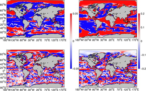
Fig. 3 As in Fig. 2, but for the intermediate layer.

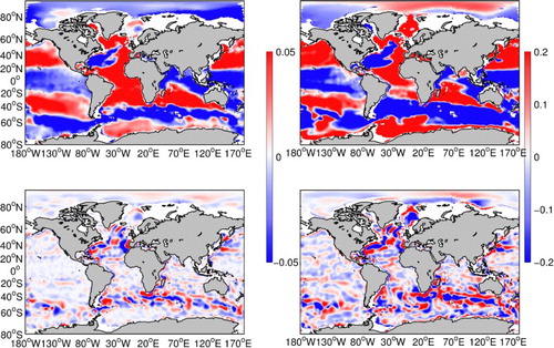
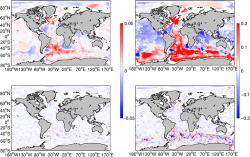
Fig. 4 As in Fig. 2, but for the deep layer.

Around the North Pole, PE displays salty and warm biases in the top layer. The bias in temperature decreases close to the Arctic shelves and Beaufort Sea, while the bias in salinity changes sign (too fresh). There is also a salty bias in SE but with a smaller magnitude, whereas the temperature bias is significantly reduced. However, because spectral nudging is not applied in the top 50 m in the Arctic, the temperature and salinity biases for the top 50 m from SE resemble those from PE (not shown). Hence, most of the differences between the two experiments come from depths below 50 m. In the Antarctic, PE also shows mostly salty and warm biases; again spectral nudging reduces the biases significantly. For the other oceans, the warm and cold temperature biases tend to co-exist in PE, with a markedly warm and slightly salty bias along the equatorial wave-guides and the North Pacific. The bias in SE has much smaller spatial scales and magnitude than in PE. In SE, the regions of stronger bias (positive and negative) in the surface layer are the equator, the Southern Ocean, the western mid-latitude Pacific, the Northwest Atlantic and the Nordic Seas (i.e., presumably where the variability is the strongest).

For the intermediate layer, the patterns of salinity and temperature biases in PE are consistent with each other in general, except in the Arctic. The Southern Ocean, tropical Pacific, and the subtropical gyre in the Atlantic suffer from a cold and fresh bias, whereas the bias in most of the Atlantic Ocean, the North and South Pacific oceans and the Weddell Sea in Antarctica is the reverse. A similar relationship holds in SE between the salinity and temperature biases but at much smaller spatial scales. Again spectral nudging significantly reduces biases. The regions of stronger bias are known areas of large ocean variability (i.e., the Gulf Stream, the Kuroshio, and the Antarctic Circumpolar Current).

For the deep layer, it is clear that spectral nudging consistently reduces model biases. The warm and salty bias in PE is mostly visible in the Atlantic and the Southern Ocean, with a smaller cold and fresh bias in the other oceans. In SE, only the Antarctic Circumpolar Current region has discernible biases.

b Comparison Between the Modelled Currents and Climatological Current Meter Data

The mean “topostrophy” is used to provide a large-scale sense of currents. Topostrophy (Holloway et al., 2007) is a diagnostic tool which reduces the sense of the flow field to a scalar, capturing the dominant type of motion for a basin, if calculated as a spatial integral. High positive topostrophy is equivalent to strong cyclonic flow along steep topography, with the shallow depths to the right in the northern hemisphere. Here we use topostrophy as defined by Holloway (2008) to investigate the circulation systems from the two experiments.(3) where γ is the topostrophy, f is the (vertical) Coriolis vector; f is the Coriolis parameter; is the velocity, and is the gradient of bathymetry. Topostrophy has been used in several studies to examine model circulations (Holloway, 2008; Karcher, Kauker, Gerdes, Hunke, & Zhang, 2007; Käse, Serra, Köhl, & Stammer, 2009; Maltrud & Holloway, 2007; Nguyen, Menemenlis, & Kwok, 2011; Wang, Holloway, & Hannah, 2011; Zhang & Steele, 2007).

A total of 18,588 climatological points were compiled by Holloway et al. (2011), which provides a climatological sense of circulation in the global ocean at different depths. The averaged velocities from the 47-year model results are defined as the modelled climatological currents in the global ocean from the two runs. The modelled currents were interpolated onto the observed locations (longitude, latitude, depth) in order to compare the modelled velocities with the observed ones. In the comparison, the points with observed current speeds less than 1 cm s⁻¹ were not used because of a concern over the validity of data collected with some instruments. Some observational points fall onto land in this 1-degree z-level model, and they are ignored. A total of 6487 points were, therefore, used in the comparison.

The observed global mean from the 6487 points is 0.27 ± 0.009 (mean ± one standard error), and the global means for PE and SE are 0.18 ± 0.010 and 0.20 ± 0.009, respectively. It is expected that the two model runs would underestimate the topostrophy because of the diffusive nature of coarse-resolution models, which prevents the models from obtaining strong, narrow currents, such as boundary currents (e.g., the Gulf Stream and the Kuroshio Current), thus reducing a model's ability to accurately represent topostrophy. A statistical test indicates that, at the 95% confidence level, SE and PE have the same skill in representing topostrophy in the global mean sense.

The currents vary significantly from the sea surface to the bottom. It is desirable to further compare the mean topostrophy from model results and observations at different depth ranges (Table 1). The choice of the depth ranges is somewhat empirical and subjective. In the open mid-latitude ocean, the 200–1000 m layer can represent the permanent pycnocline that separates the upper layer (<200 m) from the deep one (>1000 m). The deep ocean is further divided into two ranges (1000–2000 m and >2000 m) to better show the difference between the two experiments. Nevertheless, the division of the top 1000 m into more layers (<100, 100–200, 200–300, 300–500, and 500–1000 m) does not change the conclusions, thus the results for these layers are not shown.

Table 1. Observed and modelled topostrophy at different ranges of depth.

Depth range (m)		<200	200–1000	1000–2000	>2000
Number of points		2169	2043	817	1458
Topostrophy	OBS	0.25±0.016	0.25±0.017	0.34±0.024	0.34±0.018
	PE	0.23±0.017	0.18±0.017	0.25±0.027	0.06±0.020
	SE	0.22±0.016	0.16±0.017	0.18±0.027	0.27±0.019

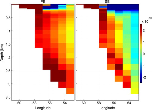
The topostrophy shows a substantial increase at depth (Table 1). The highest topostrophy for observations is located below 1000 m. SE is closer to the observed topostrophy below 2000 m (0.27 compared with 0.34) at the 95% confidence level; however, PE only produces a topostrophy of 0.06 below 2000 m. Both PE and SE achieve observed topostrophy in the upper 200 m; PE and SE are similar between 200 and 2000 m at the 95% confidence level. Thus, the improvement brought about by SE is achieved for depths lower than 2000 m. This improvement can be attributed to the reduced biases in the SE horizontal density gradient. Here we choose a section in the Labrador Sea at 57.2°N and from 61°W to 53°W. The density fields for this section for model simulations averaged over the study period and the combined climatology averaged over 12 months were computed. The differences in the modelled and observed density gradients are shown in Fig. 5. It is clear that the biases in density gradients are greatly reduced in SE, particularly for the deep layer (deeper than 2000 m) over the lower continental slope and rise.

Fig. 5 Horizontal density gradient differences between model simulations averaged over the study period and the combined climatology averaged over 12 months for the 57.2°N section in the Labrador Sea. The left panel is for PE and the right panel for SE. The horizontal density gradient is computed as the difference in the density between the two adjacent cells divided by the distance (positive direction is eastward). Units are kg m⁻⁴.

4 Variability of the ocean surface quantities obtained by PE and SE

The atmosphere is one of the main driving forces of the global oceans through heat, freshwater, and momentum fluxes at the ocean surface. Because the ocean surface is directly connected to the atmosphere, accurate SST in ocean models is a key variable in coupled atmosphere–ocean models (e.g., climate models). An important indicator of the heat content of the top 400 m of the global ocean is SSH (Dong & Kelly, 2004; Ferry, Reverdin, & Oschlies, 2000; White & Tai, 1995). Changes in SSH are closely linked to climate changes. Variations in SSH and SST from the two experiments were investigated and compared with observations to examine the effects of spectral nudging.

Major signals at large scales can be captured by the leading modes of the EOFs. Previous studies have linked the principal components (PCs) to major climate events, such as the El Niño–Southern Oscillation (ENSO) and the North Atlantic Oscillation (NAO). Well-represented PCs by ocean models are often used in studies focusing on linkages between variations in oceans and atmospheric systems (e.g., Wang et al., 2014). The EOF approach was used to investigate the temporal and spatial variations of SSH and SST at the global scale for periods when global observational data were available. However, the satellite data record is not sufficiently long to address decadal variability; therefore, long time series from specific locations were used to address interannual to decadal variability.

a Variations in SSH

1 Comparison with altimeter data

Figure 6a shows the first and second EOF patterns from the altimeter data, PE, and SE. The first modes explain 23, 30, and 32% of the total variance in the data, PE, and SE, respectively, and the second modes 8, 12, and 13%, respectively. Both the PE and SE demonstrate encouraging skills in capturing the first two modes of the observed SSH. The EOF patterns from the observations and the two model experiments are consistent with each other in general, though some subtle differences are noticeable in magnitude. The EOF1s from the three sources display negative anomalies in the western Pacific equatorial zone and positive ones in the eastern segment and in the Indian Ocean. Slight differences in magnitude are seen among the patterns of EOF1. The negative anomalies in the equatorial region in the observational EOF2 are well captured by both PE and SE, with the former performing slightly better. The positive anomalies in the eastern equatorial Pacific Ocean shown in the observed EOF2 are not well captured by the experiments. The observed positive anomalies in the western equatorial Pacific Ocean or in the Indian Ocean are not simulated well by SE, while PE shows much better agreement with observations. Though PE slightly outperforms SE in some isolated regions, the frequency-dependent nudging approach used in the latter still shows good skill in representing the two leading EOF patterns.

Fig. 6 (a) The EOFs of SSH from altimeter data, PE, and SE simulations; (b) the corresponding PCs. Units are m.

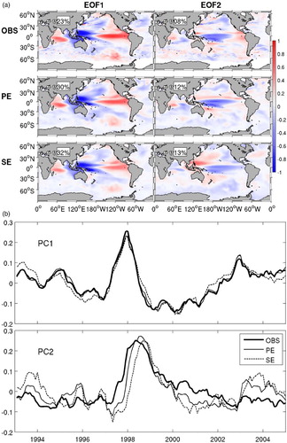
Figure 6b shows the principal components PC1 and PC2 from altimeter data, PE, and SE. The PCs from the three sources agree well with each other in general; however, small differences exist, especially in PC2. The PC1 from PE and SE is well correlated with that of the altimeter data (0.99 and 0.94, respectively, significant at the 95% confidence level). The PC2 of PE is better correlated with that of the observations than that of SE (0.82 compared with 0.55, both significant at the 95% confidence level).

2 Comparison with tide-gauge data and steric height anomalies

In order to address the interannual and decadal variability of SSH, long-term measurements at specific locations were used. Two locations in the North Atlantic, one in the Pacific, and one in the Indian Ocean were chosen, all covering the 1958–2004 simulation period, though with some gaps. The data and model outputs are averaged annually. In the North Atlantic, the Labrador Sea plays an important role in the global climate system for deep water formation. Hence, station Bravo in the Labrador Sea was chosen to examine long-term variations in sea level presented in the two model runs. Sea level variations at Bermuda in the subtropical North Atlantic Ocean are also discussed. Figure 7 shows the sea level anomalies at Bermuda (top panel) from the two model runs and tide-gauge measurements. The bottom panel shows the steric height anomalies (a good measure for variations in SSH) at the World Ocean Circulation Experiment (WOCE) station Bravo and the sea level anomalies from the two model runs. Steric height data were reconstructed using T-S data from various sources (WOCE and regular surveys from the Bedford Institute of Oceanography) provided by Yashayaev (2007).

Fig. 7 Sea level anomalies at (top panel) Bermuda and (bottom panel) station Bravo from model results, tide-gauge data, and steric height observations.

The variations in SSH at Bermuda from both experiments are similar to the observed variations. They both miss the lowest observed sea level event in 1970 and second lowest in 1973 though PE is slightly closer to the observation than SE in 1970, and SE performs somewhat better in 1973. These results demonstrate that the model's skill depends on the time period. The correlation coefficients between the modelled and observed SSH are 0.67 and 0.60 (both significant at the 95% confidence level) for PE and SE, respectively.

At station Bravo, both models show some skill in representing variations in steric height, and the model's skill again depends on the time period. The correlation coefficients between modelled SSH and observed steric height are 0.50 (p = 0.001) and 0.30 (p = 0.15) for PE and SE, respectively.

In the Pacific, ENSO is a major climatic event. So a reasonable reproduction of SSH is a key criterion for evaluating model results. The tide-gauge station at Guam has a long data record, which can be used to examine the performance of the two experiments. During strong El Niño events, tide-gauge data at Guam show a large negative anomaly, or lower than average sea level. In the Indian Ocean, tide-gauge station Vishakhapatnam is used.

Figure 8 shows the time series of tide-gauge and model sea level anomalies at Guam and Vishakhapatnam. At Guam, the two experiments represent observed sea level anomalies reasonably well until the early 1990s but fail to reproduce the strong variation in the late 1990s and early 2000s. The correlation coefficients between the modelled and observed SSH are 0.58 and 0.59 (both significant at the 95% confidence level) for PE and SE, respectively.

Fig. 8 Sea level anomalies at (top panel) Guam and (bottom panel) station Vishakhapatnam from model results and tide-gauge data.

There is better agreement at station Vishakhapatnam between model results and observations for both PE and SE. The correlation coefficients between the modelled and observed SSH are 0.68 and 0.69 (both significant at the 95% confidence level) for PE and SE, respectively.

In summary, no clear improvement or degradation is achieved by implementing spectral nudging in terms of agreement with observed variations in sea level (or steric height) at these stations. Spectral nudging does not appear to affect variations in sea level at interannual and decadal time scales.

b Variations in SST

The SST is strongly constrained by air temperature; therefore, it is more constrained than SSH and less departure from the mean and less variability are expected. However, because He et al. (2014) found a greater degree of departure in PE than in SE in their SST comparison, it is felt that an equivalent comparison should be presented.

The SST data are used to investigate the performance of the two model runs. Figure 9 shows the first two EOF modes and PCs from the observations and the model results. The first modes explain 14, 18, and 17% of the total variance for the observational, PE, and SE SSTs, respectively. The second modes explain 6, 7, and 7%, respectively. The structure and variability of the first two modes of the PE and SE SSTs are similar to those of the observed SSTs. The strong positive anomalies of the observational EOF1 in the eastern equatorial Pacific Ocean are well captured by the PE and SE EOF1s, indicating that temperature variations in this region are the most prominent events in the global ocean. The observed positive anomalies in the southern Pacific Ocean are also shown in the PE and SE EOF1s. The three EOF2s are consistent with each other in general although some subtle differences in magnitude can be found. Stronger positive anomalies are produced by PE than by SE in the Pacific sector of the Antarctic Ocean. However, these are not clearly shown in observations. The PC1s of PE and SE are well correlated with that of the observed data (0.98 and 0.97, respectively, significant at the 95% confidence level). The PC2 of PE is better correlated with that of the observations than that of SE (0.96 compared with 0.90, both significant at the 95% confidence level).

Fig. 9 (a) EOFs of SST from IGOSS data, PE, and SE simulations; (b) corresponding PCs (°C).

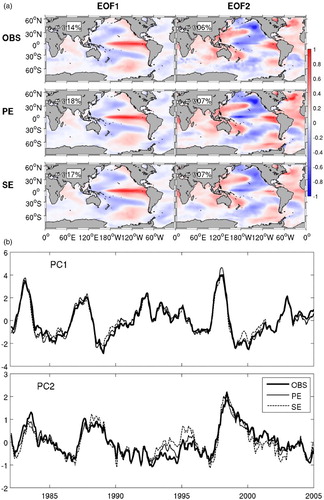
Because of the importance of the contribution of ENSO to SST variations in the equatorial Pacific, the interannual and decadal variability in long time series of SST were investigated. The extremes of this climate pattern cause extreme weather (such as floods and droughts) in many regions of the world. In the Niño 3.4 region (bounded by 120°–170°W and 5°S–5°N), there exists a long time series of observed SST dating back to 1871 (http://www.esrl.noaa.gov/psd/gcos_wgsp/Timeseries/Nino34/) that allows evaluation of model performance in terms of capturing the important climatic events at decadal time scales.

Figure 10 shows the SST anomalies from the observations and the PE and SE simulations. The observed variations in the Niño 3.4 region are well represented in PE and SE. The correlation coefficients between the modelled and observed SSTs are 0.93 and 0.90 (both significant at the 95% confidence level) for PE and SE, respectively.

Fig. 10 Time series of SST anomalies (°C) for the Niño 3.4 region from observations, PE, and SE.

The mean temperature from 1958 to 2004 in this region is 27°, 26.2°, and 26.6°C for the observed, PE, and SE, respectively.

Both models can represent SST variations in this region well. Though PE shows slightly better skill at representing the observed variations, SE has better skill at maintaining the mean SST closer to the observed SST in the Niño 3.4 region.

5 Summary and discussion

Water mass properties are the result of the interaction between the ocean and atmosphere, and advective, convective, and mixing processes in the ocean. The intent of spectral nudging is to represent unresolved processes (because of limited resolution and other factors) that maintain the long-term properties of the water masses while leaving shorter term properties and higher-frequency scales unconstrained.

1. The spectral-nudging technique helps constrain model drift in temperature and salinity in terms of the mean state, which is consistent with He et al. (2014) and Lu et al. (2007). To further this finding the regional distribution of the drift was investigated at different depths. Fresh biases are produced by PE for approximately the top 150 m in the Atlantic, Pacific, and Indian oceans. In the Arctic Ocean, the fresh bias in PE penetrates much deeper than 150 m, as deep as 500 m. The freshness of the top 500 m in the Arctic Ocean could be caused by various factors, such as sea-ice melting and river run-off. The fresh bias in the Arctic Ocean could be caused by an underestimate of the Atlantic water mass inflow, which is a common problem with coarse-resolution models, as discussed in Wang et al. (2011). In the Antarctic Ocean, the pattern of salinity biases is complicated, though a fresh bias is found in the very near-surface layer (approximately the top 50 m).

2. Spectral nudging improves model skill in representing topostrophy below 2000 m, where the prognostic model loses most of its skill. Both PE and SE represent the observed currents reasonably well in the upper 200 m. This study suggests that, for the most part, the spectral-nudging approach can help models approximate the realistic circulation in the deep ocean. Temperature and salinity biases in the prognostic model prevent the model from maintaining the density gradients in the abyssal ocean, thus failing to produce the observed topostrophy.

3. The PCs of SSH and SST from PE agree a little better with observations than SE, but the interannual and decadal variations from the two model experiments are close to each other, which suggests that applying spectral nudging in studying interannual and decadal variations of SSH and SST is appropriate. Further comparisons between tidal-gauge data and model results suggest that low-frequency (i.e., interannual and decadal) variations in SSH and SST can be reproduced reasonably well in the spectrally nudged experiment as in the fully prognostic simulation.

4. He et al. (2014) stressed that the spectral-nudging approach is not suitable for use in climate models because of the undetermined seasonal climate in the future. It is further noted here that the seasonal cycle is not well known in difficult-to-access areas. This study suggests, however, that the spectral-nudging approach can be used in studying interannual and decadal variations of the global ocean over a few decades. Hence, the climate community working at coarse resolution could benefit from improved deep-ocean properties while maintaining reasonable skill in the upper ocean for low-frequency variability. One caveat is that in climate studies involving much longer simulations, nudging to a fixed climatology could be problematic.

Acknowledgements

Z.W. is grateful to the late Dr. Daniel Gordon Wright, who supported and provided instructions for this study. Discussions with Dr. Youyu Lu helped Z.W. understand issues with the spectral-nudging approach. Dr. Blair W. Greenan's continuous support made the completion of this paper possible. The authors thank Drs. Brenda Topliss and David Greenberg and also Brendan DeTracey for their constructive comments. Critical comments from two anonymous reviewers helped improve the manuscript.

Disclosure statement

No potential conflict of interest was reported by the authors.

References

- Balmaseda, M. A., Dee, D., Vidard, A., & Anderson, D. L. T. (2007). A multivariate treatment of bias for sequential data assimilation: Application to the tropical oceans. Quarterly Journal of the Royal Meteorological Society, 133(622), 167–179. doi: 10.1002/qj.12
- Barnier, B., Madec, G., Penduff, T., Molines, J. M., Treguier, A-M., Sommer, J. L., … Cuevas, B. D. (2006). Impact of partial steps and momentum advection schemes in a global ocean circulation model at eddy permitting resolution. Ocean Dynamics, 56, 543–567. doi:10.1007/s10236-006-0082-1 doi: 10.1007/s10236-006-0090-1
- Blanke, B., & Delecluse, R. (1993). Variability of the tropical Atlantic Ocean simulated by a general circulation model with two different mixed-layer physics. Journal of Physical Oceanography, 23, 1363–1388. doi: 10.1175/1520-0485(1993)023<1363:VOTTAO>2.0.CO;2
- Boyer, T. P., Antonov, J. I., Garcia, H. E., Johnson, D. R., Locamini, R. A., Mishonov, A. V., … Smolyar, I. V. (2006). World Ocean database 2005. In S. Levitus (Ed.), NOAA Atlas NESDIS 60. Washington, D.C.: U.S. Government Printing Office.
- Brodeau, L., Barnier, B., Treguier, A.-M., Penduff, T., & Gulev, S. (2010). An ERA40-based atmospheric forcing for global ocean circulation models. Ocean Modelling, 31, 88–104. doi:10.1016/j.ocemod.2009.10.005 doi: 10.1016/j.ocemod.2009.10.005
- Chepurin, G. A., Carton, J. A., & Dee, D. (2005). Forecast model bias correction in ocean data assimilation. Monthly Weather Review, 133(5), 1328–1342. doi: 10.1175/MWR2920.1
- D'Andrea, F., & Vautard, R. (2000). Reducing systematic errors by empirically correcting model errors. Tellus A, 52(1), 21–41. doi: 10.1034/j.1600-0870.2000.520103.x
- Dietrich, D. E., Mehra, A., Haney, R. L., Bowman, M. J., & Tseng, Y. H. (2004). Dissipation effects in North Atlantic Ocean modeling. Geophysical Research Letters, 31, L05302. doi:10.1029/2003GL019015 doi: 10.1029/2003GL019015
- Dong, S., & Kelly, K. A. (2004). Heat budget in the Gulf Stream region: The importance of heat storage and advection. Journal of Physical Oceanography, 34, 1214–1231. doi:10.1175/1520-0485 doi: 10.1175/1520-0485(2004)034<1214:HBITGS>2.0.CO;2
- Ferry, N., Reverdin, G., & Oschlies, A. (2000). Seasonal sea surface height variability in the North Atlantic Ocean. Journal of Geophysical Research, 105, 6307–6326. doi: 10.1029/1999JC900296
- Fichefet, T., & Morales Maqueda, M. A. (1997). Sensitivity of a global sea ice model to the treatment of ice thermodynamics and dynamics. Journal of Geophysical Research, 102, 12609–12646. doi:10.1029/97JC00480 doi: 10.1029/97JC00480
- Gent, P. R., & McWilliams, J. C. (1990). Isopycnal mixing in ocean circulation models. Journal of Physical Oceanography, 20, 150–155. doi: 10.1175/1520-0485(1990)020<0150:IMIOCM>2.0.CO;2
- Griffith, A. K., & Nichols, N. K. (2000). Adjoint methods in data assimilation for estimating model errors. Flow Turbulence and Combustion, 65, 469–488. doi: 10.1023/A:1011454109203
- He, Z., Thompson, K. R., Ritchie, H., Lu, Y., & Dupont, F. (2014). Reducing drift and bias of a global ocean model by frequency-dependent nudging. Atmosphere-Ocean, 52(3), 242–255. doi:10.1080/07055900.2014.922240 doi: 10.1080/07055900.2014.922240
- Holloway, G. (2008). Observing global ocean topostrophy. Journal of Geophysical Research, 113, C07054. doi:10.1029/2007JC004635
- Holloway, G., Dupont, F., Golubeva, E., Häkkinen, S., Hunke, E., Jin, M., … Zhang, J. (2007). Water properties and circulation in the Arctic Ocean models. Journal of Geophysical Research, 112, C04S03. doi:10.1029/2006JC003642
- Holloway, G., Nguyen, A., & Wang, Z. (2011). Oceans and ocean models as seen by current meters. Journal of Geophysical Research, 116, C00D08. doi:10.1029/2011JC007044
- Karcher, M., Kauker, F., Gerdes, R., Hunke, E., & Zhang, J. (2007). On the dynamics of Atlantic water circulation in the Arctic Ocean. Journal of Geophysical Research, 112, C04S02. doi:10.1029/2006JC003630 doi: 10.1029/2006JC003630
- Käse, R. H., Serra, N., Köhl, A., & Stammer, D. (2009). Mechanisms for the variability of dense water pathways in the Nordic Seas. Journal of Geophysical Research, 114, C01013. doi:10.1029/2008JC004916 doi: 10.1029/2008JC004916
- Lu, Y., Wright, D. G., & Yashayaev, I. (2007). Modelling hydrographic changes in the Labrador Sea over the past five decades. Progress in Oceanography, 73, 406–426. doi: 10.1016/j.pocean.2007.02.007
- Maltrud, M., & Holloway, G. (2007). Implementing biharmonic neptune in a global eddying ocean model. Ocean Modelling, 21, 22–34. doi:10.1016/j.ocemod.2007.11.003 doi: 10.1016/j.ocemod.2007.11.003
- Myers, P. G., & Kulan, K. (2012). Changes in the deep western boundary current at 53°N. Journal of Physical Oceanography, 42, 1207–1216. doi:10.1175/jpo-D-11-090.1 doi: 10.1175/JPO-D-11-090.1
- Nguyen, A. T., Menemenlis, D., & Kwok, R. (2011). Arctic ice-ocean simulation with optimized model parameters: Approach and assessment. Journal of Geophysical Research, 116, C04025. doi:10.1029/2010JC006573 doi: 10.1029/2010JC006573
- Rattan, S., Myers, P. G., Treguie, A. M., Theetten, S., Biastoch, A., & Böning, C. (2010). Towards an understanding of Labrador Sea salinity drift in eddy-permitting simulations. Ocean Modelling, doi:10.1016/j.ocemod.2010.06.007
- Smith, R. D., Maltrud, M. E., Bryan, F. O., & Hecht, M. W. (2000). Numerical simulation of the North Atlantic Ocean at 1/10°. Journal of Physical Oceanography, 30, 1532–1561. doi: 10.1175/1520-0485(2000)030<1532:NSOTNA>2.0.CO;2
- Stacey, M. W., Shore, J., Wright, D. G., & Thompson, K. R. (2006). Modeling events of sea-surface variability using spectral nudging in an eddy permitting model of the northeast Pacific Ocean. Journal of Geophysical Research, 111, C06037. doi:10.1029/2005JC003278 doi: 10.1029/2005JC003278
- Steele, M., Morley, R., & Ermold, W. (2001). PHC: A global ocean hydrography with a high quality Arctic Ocean. Journal of Climate, 14, 2079–2087. doi: 10.1175/1520-0442(2001)014<2079:PAGOHW>2.0.CO;2
- Thompson, K., Wright, D. G., Lu, Y., & Demirov, E. (2006). A simple method for reducing seasonal bias and drift in eddy resolving ocean models. Ocean Modelling, 13, 109–125. doi:10.1016/j.ocemod.2005.11.003 doi: 10.1016/j.ocemod.2005.11.003
- Wang, Z., Holloway, G., & Hannah, C. (2011). Effects of parameterized eddy stress on volume, heat, and freshwater transports through Fram Strait. Journal of Geophysical Research, 116, C00D09. doi:10.1029/2010JC006871
- Wang, Z., Lu, Y., Dupont, F., Loder, J., Hannah, C., & Wright, D. (2014). Variability of sea surface height and circulation in the North Atlantic: Forcing mechanisms and linkages. Progress in Oceanography. doi:10.1016/j.pocean.2013.11.004
- White, B. W., & Tai, C. (1995). Inferring interannual changes in global upper ocean heat storage from TOPEX altimetry. Journal of Geophysical Research, 100, 24934–24954.
- Wright, D. G., Thompson, K. R., & Lu, Y. (2006). Assimilating long-term hydrographic information into an eddy-permitting model of the North Atlantic. Journal of Geophysical Research, 111, C09022. doi:10.1029/2005JC003200
- Yashayaev, I. (2007). Hydrographic changes in the Labrador Sea, 1960–2005. Progress in Oceanography, 73, 242–276. doi: 10.1016/j.pocean.2007.04.015
- Zhang, J., and Steele, M. (2007). Effect of vertical mixing on the Atlantic water layer circulation in the Arctic Ocean. Journal of Geophysical Research, 112, C04S04. doi:10.1029/2006JC003732
- Zhu, J., Demirov, E., Dupont, F., & Wright, D. (2010). Eddy-permitting simulation of the sub-polar North Atlantic: Impact of the model bias on water mass properties and circulation. Ocean Dynamics, 60, 1177–1192. doi:10.1007/s10236-010-0320-4 doi: 10.1007/s10236-010-0320-4