Trends and Variability in Sea Ice and Icebergs off the Canadian East Coast

ABSTRACT

Seasonal time series of sea-ice area or extent in several regions along the east coast of Canada were compiled from several sources for the period 1901 to 2013 and compared with an index of ice extent off southwest Greenland, iceberg season length south of 48°N, air temperature, and other climate indices. Trends in winter ice area and iceberg season length are significant over the past 100 years and 30 years. Variability of winter ice area and iceberg season length is associated with a combination of the North Atlantic Oscillation (NAO) and the Atlantic Multidecadal Oscillation (AMO) indices superimposed on a negative trend. Thus, large declines in ice area and iceberg season length in the 1920s and 1990s can be attributed to a decreasing NAO index and a shift to the positive phase of the AMO at the end of these decades. Ice extent in southern areas such as the Scotian Shelf is more strongly correlated with the Western Atlantic index than with the NAO. Ice area trends (in percent per decade) are larger in magnitude and account for twice as much of the variance in ice area for summer than for winter, with summer trends significant over 30-, 60- and 100-year periods. Sea-ice variability is generally consistent with air temperature variability in the various regions; in the 1930s, during the early twentieth-century warming period, ice anomalies were higher and temperature anomalies were lower along the coast of eastern Canada than along the coast of southwestern Greenland.

RÉSUMÉ

[Traduit par la redaction] Des séries temporelles de superficie ou d’étendue de glace marine, couvrant plusieurs régions le long de la côte est du Canada, ont été obtenues de diverses sources, pour la période de 1901 à 2013. Elles ont été comparées à un index d’étendue de glace au sud-ouest du Groenland, à la durée de la saison des icebergs au sud du 48^e parallèle nord, à la température de l'air et à d'autres indices climatologiques. Les tendances de la superficie de la glace hivernale et de la durée de la saison des icebergs sont significatives pour les 100 et les 30 dernières années. La variabilité de la superficie de la glace hivernale et celle de la durée de la saison des icebergs sont associées à la fois aux indices de l'oscillation nord-atlantique (ONA) et de l'oscillation atlantique multidécennale (OAM), superposés à une tendance négative. Ainsi, les diminutions importantes de la superficie de la glace et de la durée de la saison des icebergs dans les années 1920 et dans les années 1990 peuvent être attribuées à la diminution de l'indice de l'ONA et à un décalage vers la phase positive de l'OAM, à la fin de ces décennies. L’étendue de la glace dans les régions du sud, sur le plateau néo-écossais, par exemple, est plus fortement corrélée avec l'indice de l'Atlantique Ouest qu'avec l'indice de l'ONA. Les tendances de la superficie de la glace (en pour cent par décennie) sont plus élevées et présentent une variance deux fois plus forte en été qu'en hiver. Les tendances estivales sont significatives pour les périodes de 30, 60 et 100 ans. La variabilité de la glace marine correspond généralement à la variabilité de la température dans les diverses régions. Dans les années 1930, durant la période de réchauffement du début du XX^e siècle, les anomalies de glace étaient plus élevées et les anomalies de température étaient plus faibles le long du littoral est du Canada que le long du littoral sud-ouest du Groenland.

KEYWORDS:

• sea ice
• icebergs
• climate
• eastern Canada

1 Introduction

A significant decline in annual mean sea-ice extent of −4% per decade has been observed in the northern hemisphere from 1979 to 2010 (Cavalieri & Parkinson, 2012), with a larger decline in summer (−10% per decade) than in winter (−2% per decade). A longer record of summer ice extent based on terrestrial proxies suggests that the decline over the past four or five decades has been unprecedented compared with trends during the past 1450 years (Kinnard et al., 2011).

For the Baffin Bay/Labrador Sea region, summer and winter trends are −17% per decade and −7% per decade, respectively, for the 1979–2010 period (Cavalieri & Parkinson, 2012). For the 1968–2010 period, trends in summer sea-ice area are −10%, −14%, and −17% for Baffin Bay, Davis Strait, and the northern Labrador Sea, respectively (Derksen et al., 2012; Henry, 2011).

In summer, the decline in northern hemisphere sea-ice extent for the 1958–1997 period is relatively monotonic, whereas in winter the decline is superimposed on decadal variations associated with the North Atlantic Oscillation (NAO; Deser, Walsh, & Timlin, 2000). Decadal variations are also observed in winter sea-ice concentration (SIC) anomalies that are of opposite signs in the western and eastern Atlantic (Deser et al., 2000). Sea-ice extent anomalies in the Labrador Sea lag those in the Greenland Sea by about four years, consistent with the average speed of the subpolar gyre boundary currents, because positive ice anomalies are thought to correspond to negative salinity anomalies propagating with the currents (Mysak & Manak, 1989). Ice and salinity anomalies propagate cyclonically around the Labrador Sea, with ice anomalies off Newfoundland lagging those in Davis Strait by one year and ice anomalies in Davis Strait lagging salinity anomalies at Fylla Bank off southwestern Greenland by eight months (Deser, Holland, Reverdin, & Timlin, 2002).

Multidecadal fluctuations in winter-spring sea ice in the Greenland Sea are closely associated with the Atlantic Multidecadal Oscillation (AMO; Drinkwater et al., 2014; Miles et al., 2014), commonly defined as the detrended mean sea surface temperature (SST) in the North Atlantic south of 70°N. Off Newfoundland, multidecadal ice fluctuations are weaker than in the Greenland Sea and are offset from the AMO by several years (Miles et al., 2014).

Although several mechanisms have been proposed to account for the AMO, there is a common consensus that the NAO is an important driving force. Long-term positive (negative) phases of the NAO coincide with the negative (positive) phase of the AMO, generally with a lag of several years, and westerly and trade wind anomalies associated with the phase of the NAO act to reinforce the phase of the AMO (Grossmann & Klotzbach, 2009). The NAO is characterized by strong decadal variability during the negative AMO phase and weak decadal variability during the positive AMO phase (Walter & Graf, 2002).

Modelling studies suggest that negative feedbacks associated with a persistent NAO anomaly lead to a phase reversal of the AMO. A persistent positive NAO signal during the negative AMO phase has been shown to result in a strengthened Atlantic Meridional Overturning Circulation (AMOC) through an increase in deep-water formation because of cooling in the Labrador Sea (e.g., Robson, Sutton, Lohmann, Smith, & Palmer, 2012). The strengthened AMOC leads to enhanced northward heat transport, warming of the North Atlantic, and transition to the positive phase of the AMO, with the largest SST anomalies occurring in the subpolar gyre. A warm subpolar gyre and reduced south-to-north SST gradient lead to weakened North Atlantic trade winds and northward ocean heat transport across the equator, reinforcing the positive AMO phase (Smith et al., 2010). It has been suggested that a strengthened AMOC, in addition to increased greenhouse gas-induced global warming, might have contributed to the observed decline in winter sea ice in the Labrador and Nordic seas in recent decades (Mahajan, Zhang, & Delworth, 2011). The propagation of Great (low) Salinity Anomalies from the Greenland Sea to the Labrador Sea due to a persistent negative NAO signal during the positive phase of the AMO may have a role in the transition to the negative phase of the AMO (Zhang & Vallis, 2006). Volcanic and anthropogenic aerosols may also contribute to multidecadal Atlantic climate variability (e.g., Booth, Dunstone, Halloran, Andrews, & Bellouin, 2012).

In a study of winter atmospheric teleconnection patterns in the northern hemisphere, Wallace and Gutzler (1981) showed that sea level pressure statistics are dominated by negative correlations between polar and temperate latitudes, such as those associated with the NAO. However, 500 hPa statistics are dominated by patterns of a more regional scale, such as the Western Atlantic (WA) pattern, which consists of a dipole with centres at 55°N, 55°W and 30°N, 55°W. The WA pattern has been linked to SST variability east of Newfoundland (Deser & Blackmon, 1993).

As part of a study under the Aquatic Climate Change Adaptation Services Program (ACCASP) of Fisheries and Oceans Canada (DFO), records of sea-ice area and extent off the east coast of Canada were compiled from several data sources (Peterson & Pettipas, 2013). In this paper, trends and variations in sea-ice extent and area since the late 1800s are presented for four regions off the east coast of Canada and compared with the same parameters off southwestern Greenland; in addition, they are compared with air temperature and atmospheric indices, as well as the AMO. Significant correlations have previously been found between sea-ice severity and air temperature off Newfoundland (Prinsenberg, Peterson, Narayanan, & Umoh, 1997) and in the Gulf of St. Lawrence (Galbraith, Hebert, Colbourne, & Pettipas, 2013). Trends in iceberg numbers off eastern Newfoundland (at 48°N) are also presented because iceberg numbers are highly correlated with sea-ice extent (Smith, 1931).

2 Data sources

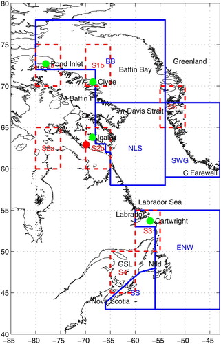
Records of sea-ice area or extent were compiled for four areas off the east coast of Canada: Baffin Bay (BB: 68°–78°N), Northern Labrador Sea (NLS: 58°–68°N), East Newfoundland Waters (ENW: 43°–55°N), and the Scotian Shelf (SS: east of Cabot Strait), as well as southwestern Greenland (SWG) (Fig. 1).

Fig. 1 Map of the northwest Atlantic showing the five sea-ice regions (blue polygons), seven air temperature grid squares (dashed red squares), paleoclimate temperature site (red dot), and communities referred to in the text (green dots); GSL: Gulf of St. Lawrence, Nfld: Newfoundland.

For the BB and NLS regions, monthly sea-ice area was computed from mid-month sea-ice concentration fields in the Hadley Centre Global Sea Ice and Sea Surface Temperature (HadISST1) dataset (Rayner et al., 2003) that, for the 1901–1978 period, is based mainly on the end-of-month dataset of Walsh and Chapman (2001). Much of the Walsh and Chapman data before 1953 is either climatological or interpolated data and, therefore, must be used with caution. Sea-ice area was computed for four seasons: winter, spring, summer, and autumn, as in Cavalieri and Parkinson (2012). Data for 1870–1900 and 1940–1952 were not used because the fields were set to monthly climatology during those periods. Data were also not used for winter and autumn 1901–1939 because it appeared that SIC in many grid squares was set to climatology in many of these months as well.

For the period after 1978, the HADISST1 dataset is based on passive microwave data that have a large footprint; therefore, the dataset is hampered by land contamination in coastal areas (Rayner et al., 2003). Therefore, for months when data were available during the 1969–2011 period, monthly mean sea-ice area computed from the Canadian Ice Service Digital Archive regional (CISDA-R) dataset (Tivy et al., 2011) was used instead.

For the ENW and SS regions in late winter/early spring (February–April), the sea-ice extent datasets of Hill (1999) and Hill, Ruffman, and Drinkwater (2002) were used and updated to 2013 using the CISDA-R dataset (for periods of overlap between the Hill and CISDA data, the Hill data were used because they were in good agreement with the CISDA data). The main source of information for the SS dataset is ship-based observations before the 1950s and ice charts after. However, ice in the SS region originates in the Gulf of St. Lawrence where ice data are sparse before the introduction of ice charts in the late 1950s. In the SS region, linear regression was used to estimate missing data for individual months using data from other winter months of the same year.

For SWG in summer, sea ice is commonly referred to as “storis” (i.e., ice that has drifted southward in the East Greenland Current and around Cape Farewell). To compare with ice area off eastern Canada, the monthly storis index dataset from Rosing-Asvid (2006) was used. The summer value was computed as the mean of the May–July indices, as in Schmith and Hansen (2003).

A dataset of the monthly and annual numbers of icebergs drifting south of 48°N off eastern Newfoundland is produced by the International Ice Patrol from data collected under the auspices of the US Coast Guard (Anderson, 1993; U.S. Coast Guard, 2014). This information comes mainly from ship-based observations from 1900 to 1945, aerial visual observations from 1946 to 1983, and aerial visual and radar observations with model output from 1983 to the present. In recent decades, many of the sightings were collected by the Canadian Ice Service and Provincial Aerospace Ltd. The annual flux of icebergs provided in the dataset is defined as the total flux from October to September. We computed the season length south of 48°N as the total number of months from October to September with at least one iceberg (all months with no icebergs were excluded).

Air temperature data were obtained from the CRUTEM4 dataset, developed by the Climatic Research Unit (University of East Anglia) in conjunction with the Hadley Centre (at the UK Met Office) (Jones et al., 2012). Data were used from several grid squares representing the five sea-ice regions, each square being 5° latitude by 5° longitude (Fig. 1). For each of the ENW, SS, and SWG regions, a single grid square having a long time series was chosen (S3, S4, and S5). However, for BB and NLS two squares were chosen because the datasets had more missing data (S1 and S2). To extend the S2 data back in time, a summer temperature reconstruction based on lake sediments from Upper Soper Lake in southern Baffin Island (Hughen, Overpeck, & Anderson, 2000) was also included.

3 Sea-ice extent and area

The time series of seasonal sea-ice area anomalies in BB and NLS and ice extent anomalies in ENW and SS for winter and summer are plotted in Fig. 2. The reference period used to compute anomalies is 1961 to 1990, as in Bush, Loder, James, Mortsch, and Cohen (2014).

Fig. 2 Ice area or extent anomalies for (left) winter and (right) summer, using1961–1990 as a reference period. Anomalies of ice area for winter (January–March) and summer (June–September) are given for BB and NLS, and of ice extent for winter (February–April) are given for ENW and SS. The anomaly of the ice extent index for summer (May–July) is given for SWG. The blue and red lines show the unsmoothed and 5-year running means, respectively.

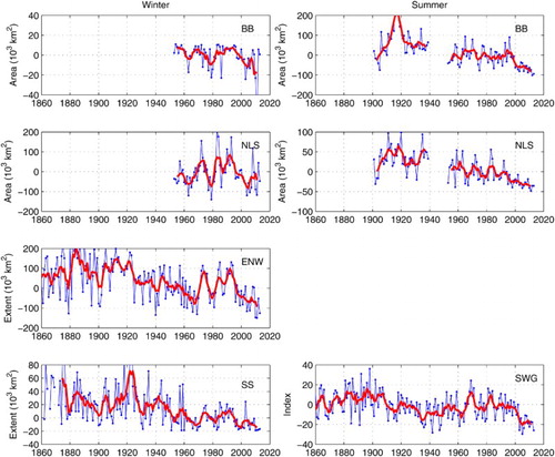
In winter, the ice area anomalies for BB are small because the enclosed area is often nearly ice covered. From the 1970s to 1990s, a decadal-scale variation can be seen in all four regions, especially NLS and ENW. Since the mid-1990s, there has been a negative trend in ice area. For ENW and SS, sea-ice extent decreased from the early 1920s to the 1960s. Sea-ice extent was high in ENW from the 1880s to 1920s, whereas SS ice extent from the 1880s to the 1910s was generally lower than in the early 1920s. Decadal-scale variations can be seen in ENW for the 1900–1925 period, which like the 1970–1995 period, corresponds to the negative phase of the AMO (Enfield, Mestas-Nunez, & Trimble, 2001).

In summer, 5-year mean ice area anomalies in BB are near zero and relatively stable for 1953 to 2000, after which there is an abrupt shift to negative anomalies. Ice area is generally higher from 1900 to 1939 than in later years, especially the 1916–1918 period. In NLS, summer ice anomalies have shown a negative trend since the early 1980s, and decadal-scale variations are in phase with those for winter anomalies but are weaker in amplitude. Similar to BB, ice area is generally higher from 1900 to 1939 than in later years, especially during the 1910–1920 period and the late 1930s. However, in SWG, 5-year mean ice extent anomalies are near zero or negative from the 1920s to the late 1960s.

Ice (storis) extent in SWG decreased significantly in 2003 and has remained below normal since then. Summer storis extent is significantly correlated with Fram Strait ice export with a lag of 0–1 years (Schmith & Hansen, 2003). Ice export was low in 2003 and 2004 (Kwok, 2009), in agreement with the decrease in storis extent in 2003. However, in spite of a return to stronger southward export of ice from Fram Strait from 2005 to 2011, based on surface pressure differences (Smedsrud, Sirevaag, Kloster, Sorteberg, & Sandven, 2011), storis anomalies have remained low. Sea surface height anomalies in the subpolar gyre centred southeast of Greenland were also extremely high in 2003 and 2004 (Mahajan et al., 2011), suggesting weaker southward ice fluxes off southeastern Greenland in those years.

Overall, the decadal-scale variations can be seen propagating around the Labrador Sea from Greenland to the Scotian Shelf, with a lag of one to several years, in agreement with Deser et al. (2002). In SWG this was seen in the summers of 1968–1971, 1981–1984, and 1989–1993, with the first peak corresponding to the Great Salinity Anomaly (Dickson, Meincke, Malmberg, & Lee, 1988). In NLS winter peaks occur in 1972–1973, 1983–1984, and 1990–1993. In ENW winter peaks occur in 1972–1976, 1984–1985, and 1990–1994, and in SS peaks occur in 1974–1975, 1985–1986, and 1989–1994.

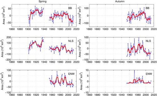
Ice-area anomalies for BB, NLS, and ENW in spring and autumn 1953–2011 are plotted in Fig. 3. For BB, there is an abrupt shift to negative anomalies after 2000, as in summer (Fig. 2). Decadal-scale variations in the 1970s to 1990s are evident for NLS and ENW, and anomalies have been relatively low since the mid-1990s in both areas in spring and autumn.

Fig. 3 Ice area anomalies in BB, NLS, and ENW for (left) spring (April–June) and (right) autumn (October–December). The blue and red lines show the unsmoothed and 5-year running means, respectively.

There also appears to be some evidence of quasi-biennial variations, such as for ENW in winter in the 1950s and 1960s. Venegas and Mysak (2000) found that quasi-biennial (2- to 2.5-year) peaks in Arctic sea-ice concentration and sea level pressure were significant at the 90% and 95% levels, respectively.

4 Icebergs

The iceberg season length and the annual flux of icebergs past 48°N are shown in Fig. 4. The season is longest in the 1910s and early 1920s, with decadal variations from the 1970s to 1990s, similar to the pattern for ice extent in ENW.

Fig. 4 (top) Annual iceberg season length anomaly, (middle) iceberg flux past 48°N anomaly, and (bottom) number of extreme observations of icebergs (October–September). The blue and red lines show the unsmoothed and 5-year running means, respectively. In the bottom panel, the shaded area represents the recent period not covered by the dataset.

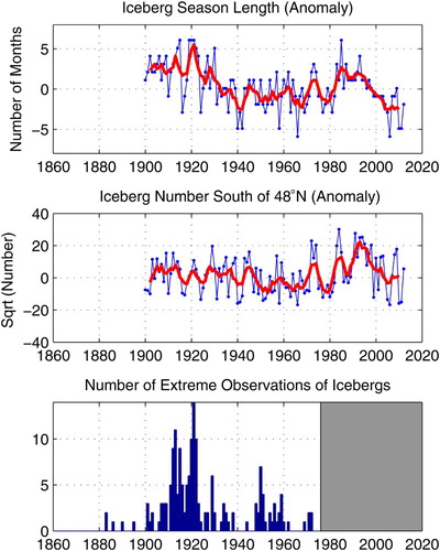
The annual iceberg flux also shows decadal-scale variations; however, unlike the length of the iceberg season, fluxes are not particularly high in the 1910s and 1920s, and values are highest after 1980. There is likely to be high uncertainty in long-term trends of iceberg fluxes because of changes in iceberg detection technology, search effort, and reporting. The main objective of the International Ice Patrol dataset is to define the area where icebergs are present and not to obtain an accurate count of all icebergs (Anderson, 1993).

Also shown in Fig. 4 is the annual number of extreme observations of icebergs (i.e., the total number of icebergs beyond the monthly climatological maximum distribution; U.S. Department of Commerce, 1974). The values are highest in the 1910s and 1920s and low in the early 1940s and 1960s, similar to the pattern for the length of the iceberg season.

5 Sea-ice and iceberg trends

For sea-ice area or extent and iceberg season length shown in Figs 2 to 4, 100-, 60-, and 30-year trends were computed for three periods: 1900–2011, 1953–2011, and 1980–2011 (Table 1). Most trends are negative, though not all are statistically significant (all trends and correlations throughout this paper are based on unfiltered data, that is, without 5-year averaging). The magnitudes of the trends in percent per decade are highest in summer and lowest in winter. The magnitudes also increase from north to south. In general, the magnitudes of the trends are highest and significant at the 5% level for the 1980–2011 period, are lowest for the 1953–2011 period and not significant at the 5% level except in summer, and are significant for the 1900–2011 period. The correlation coefficients indicate that the trend accounts for less than 25% of the variance in winter for all three periods in all areas. However, it accounts for more than 40% of the variance for the 1900–2011 and 1980–2011 periods for the NLS region in summer and for 1980–2011 in autumn.

Table 1. Trends (T) in sea-ice area for the BB, NLS, ENW, and SS regions (percent per decade) and iceberg season length south of 48°N, iceberg season length (ISL; months per decade); correlation coefficients (r) of ice area with linear trends are also shown. The three numbers in each cell refer to the periods 1900–2011, 1953–2011, and 1980–2011, respectively. Winter is January–March; Spring is April–June; Summer is July–September; Autumn is October–December. For the ENW and SS regions in winter, ice extent was used instead of ice area and the time period was February–March. Trends and correlation coefficients significant at the 5% level are shown in bold.

		Winter			Spring			Summer			Autumn
		1900–2011	1953–2011	1980–2011	1900–2011	1953–2011	1980–2011	1900–2011	1953–2011	1980–2011	1900–2011	1953–2011	1980–2011
BB	T	–	−0.5	−1.3	−0.6	−0.3	−3.1	−5.5	−6.8	−16.8	–	0.2	−6.4
	r	–	−0.35	−0.43	−0.36	−0.10	−0.53	−0.57	−0.37	−0.51	–	0.02	−0.45
NLS	T	–	0.0	−8.8	−2.9	−2.6	−10.3	−6.5	−11.2	−25.5	–	−2.5	−20.5
	r	–	0.00	−0.43	−0.57	−0.29	−0.60	0.63	−0.51	−0.65	–	−0.11	−0.68
ENW	T	−4.0	−2.9	−16.5	–	−6.2	−19.9	–	–	–	–	1.5	−34.8
	r	−0.43	−0.14	−0.49	–	−0.24	−0.43	–	–	–	–	0.01	−0.51
SS	T	−7.5	−8.0	−21.4	–	–	–	–	–	–	–	–	–
	R	−0.45	−0.20	−0.35	–	–	–	–	–	–	–	–	–
ISL	T	−0.3	−0.1	−1.5
	r	−0.39	−0.07	−0.57

Trends for iceberg season length south of 48°N show a similar pattern to ice area and extent. The trends are negative for all three periods, and the magnitude of the trends is highest for the 1980–2011 period, lowest and not significant for the 1953–2011 period, and significant for the 1900–2011 period.

6 Air temperature

Seasonal mean air temperature anomalies for winter and summer from the CRUTEM4 dataset for the five air temperature areas, S1–S5 (Fig. 1) are plotted in Fig. 5. For S1 and S2, the two grid squares are plotted as separate but overlapping lines.

Fig. 5 Seasonal air temperature anomalies from the CRUTEM4 dataset for (left) winter (December–February) and (right) summer (June–August) for grid squares S1–S5 in Fig. 1, with the y-axis inverted. The blue and red lines show the unsmoothed and 5-year running means, respectively. The reconstructed air temperature (5-year running mean) from Upper Soper Lake paleoclimate data is shown in green.

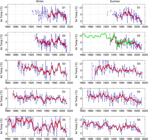
In general, the air temperature anomaly patterns from CRUTEM4 are very similar to those for sea ice. Winter air temperature anomalies are generally lower at S3 than at S4 from 1880 to 1920, consistent with higher ice anomalies for ENW than for SS. In addition, decadal variations from the 1970s to 1990s are stronger at S3 than at S4, consistent with ice anomalies for ENW and SS. From about 1925 to 1945, 5-year mean winter air temperature anomalies were generally positive at S5 but negative at S2 and S3. A positive air temperature gradient between eastern Canada and Greenland was also shown by Wood and Overland (2010) for the 1920–1939 period. The large increase in winter air temperature at S5 in the mid-1920s corresponds to a large decrease in ENW ice extent (Fig. 2) and iceberg season length (Fig. 4).

In summer, good agreement is seen between air temperature anomalies at S2 from CRUTEM4 and from the paleoclimate dataset (Hughen et al., 2000). The large increase in summer air temperature in the late 1940s can be seen in many other paleoclimate records from northeastern Canada (Overpeck et al., 1997). The anomalies are low before the mid-1940s, especially from the 1910s to 1920s when ice area anomalies at BB and NLS were high. As in winter, summer air temperature anomalies in Greenland at S5 during the 1925–1945 period were generally higher than in eastern Canada at S2 and S3.

For the 1950–2010 period, Bush et al. (2014) found that winter temperature trends in eastern Canada were generally low and not significant except at Clyde (S1). However, summer trends were positive and significant at Clyde, Iqaluit, Cartwright, and northern Nova Scotia (S1–S4). This is consistent with plots of air temperature at S1 to S4 (Fig. 5) and with ice area trends for the 1953–2011 period (Table 1). Plots of air temperature at S1 are also consistent with the study of Hamilton and Wu (2013) showing that positive mean annual temperature trends at Pond Inlet and Clyde were significant at the 10% level during the 1998–2010 period but not during the 1950–1997 period.

Seasonal mean air temperature anomalies for spring and autumn from the CRUTEM4 dataset for the five areas S1–S5 (Fig. 1) are plotted in Fig. 6. At S1–S3, 5-year mean air temperature anomalies are generally positive after the mid-1990s in spring and autumn. This is in agreement with negative ice area anomalies for NLS and ENW after the mid-1990s but differs from ice area anomalies in BB which remain high until after 2000. In autumn, air temperature anomalies at S3 are higher, and ice area anomalies in ENW are lower in the 1950s and 1960s than in the 1970s to 1990s.

Fig. 6 Seasonal air temperature anomalies from the CRUTEM4 dataset for (left) spring (March–May) and (right) autumn (September–November) for grid squares S1–S5 in Fig. 1, with the y-axis inverted. The blue and red lines show the unsmoothed and 5-year running means, respectively.

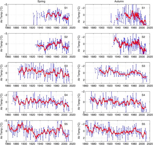
For the 1950–2010 period, Bush et al. (2014) found that spring temperature trends in eastern Canada were generally low and not significant; however, autumn trends were positive and significant at Clyde, Iqaluit, and Cartwright and of mixed significance in northern Nova Scotia. This is consistent with plots of air temperature anomalies at S1–S4 (Fig. 6). Spring ice area trends for the 1953–2011 period were also not significant for two of the three areas (Table 1). Although autumn ice area trends were also not significant, air temperature trends were significant (Bush et al., 2014). This is probably due, in part, to the 1-month difference in the autumn season definition for ice (October to December) relative to air temperature (September to November), so that autumn ice area would be affected by December atmospheric conditions.

7 Atmospheric and SST indices

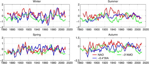
Seasonal station-based NAO (Hurrell, 1995) and AMO (Enfield et al., 2001) anomalies are plotted as 5-year running means in Fig. 7. The WA index (Wallace & Gutzler, 1981) is also shown and represents the difference in normalized 500 hPa geophysical height (GPH) between the Labrador Sea (55°N, 55°W) and the Sargasso Sea (30°N, 55°W), while the NAO represents the difference in normalized sea level pressure between Lisbon, Portugal (∼39°N, 10°W) and Stykkisholmur or Reykjavik, Iceland (∼65°N, 22°N). Like the negative NAO, the positive WA corresponds to a weak jet stream over the Atlantic, a weak Icelandic Low, and weak Subtropical High. However, it is based on data from the western Atlantic, whereas the NAO is based on data from the eastern Atlantic, about 10° further north. Although the winter WA is quite similar but inversely correlated to the NAO (Wallace & Gutzler, 1981), there are some notable differences, such as in the early 1950s and 1960s (Fig. 7). The sea level pressure patterns (not shown) indicate that a high (low) inverted WA relative to the NAO, such as during the 1961–1965 (1950–1954) period, corresponds to a southwestward (northeastward) shift in the Icelandic Low.

Fig. 7 Seasonal NAO, WA (inverted), and AMO (inverted) anomalies shown as 5-year running means for winter (December-February), spring (March-May), summer (June-August), and autumn (September-November). NAO index data provided by the Climate Analysis Section, National Center for Atmospheric Research, Boulder, Colorado, USA, Hurrell (1995); AMO (Enfield et al., 2001) data, and GPH data from the Twentieth Century Reanalysis (Compo et al., 2011) used to compute WA were provided by the National Oceanographic and Atmospheric Administration, Climate Prediction Center.

The WA was computed as(1)

using 500 hPa GPH data (z) from the Twentieth Century Reanalysis (Compo et al., 2011). However, the GPH data were not normalized (by subtracting the monthly mean and dividing by the standard deviation) as in Wallace and Gutzler (1981), so that the WA index used here reflects the zonal geostrophic wind component.

During winter, a large NAO anomaly occurs prior to the onset of positive AMO phases in the 1920s and 1990s, and a large negative NAO anomaly occurs prior to the onset of the negative AMO phase in the late 1960s. Decadal variations in the winter NAO can be clearly seen, with peaks in the 1970s, 1980s, and 1990s, as is the case for winter NLS ice area, ENW ice extent, and S2 air temperature. Quasi-decadal variations can also be seen in the winter WA during the 1945–2000 period. However, the period appears to be longer than for the NAO, with peaks in the 1960s, 1970s, and early 1990s, as is the case for SS ice extent and S4 air temperature.

During spring, NAO anomalies in the 1930s and 1940s are negative and correlated with positive air temperature anomalies at S2 and S5, whereas inverted WA anomalies during the same period are generally positive, and air temperatures at S3 and S4 are negative. Inverted WA anomalies and air temperatures at S3 and S4 also show similar patterns for autumn although the WA appears to have more of a long-term trend. In summer and autumn, air temperature variability appears to show high correspondence with the AMO.

Correlations of detrended ice area or extent with the detrended NAO, WA, and AMO (without 5-year averaging) are shown in Table 2. For BB and NLS, the correlation between winter ice and the winter NAO is stronger than with the WA, but for ENW and SS the correlation with WA is stronger than with the NAO. The correlation with the AMO is significant in all regions except BB and for both 50- and 100-year periods. In summer, the correlation with the winter NAO is not significant for either BB or NLS, but the correlation with the winter WA is significant for NLS. Correlations of summer ice area with the AMO are significant for the 50-year but not the 100-year period. In autumn, correlations with the NAO and AMO are significant (except between ENW and NAO), but correlations with the WA are not significant.

Table 2. Correlation coefficients of detrended ice area or extent at BB, NLS, ENW, and SS with the detrended winter NAO and WA (DJFM), and seasonal mean AMO for 1953–2011 (and 1900–2011 in italics). The definitions of the time periods are as in Table 1. For BB and NLS in winter, the NAO, WA, and AMO in December to February were used. Correlations of iceberg season length (ISL) and annual iceberg flux (IF) with the winter NAO, WA, and AMO are also shown. Correlations in bold are significant at the 5% level.

	Winter Ice			Spring Ice			Summer Ice			Autumn Ice
	NAO	WA	AMO	NAO	WA	AMO	NAO	WA	AMO	NAO	WA	AMO
BB	0.50	−0.16	−0.18	0.24 0.13	0.04 0.05	−0.24 −0.09	−0.06 −0.09	0.13 0.07	−0.27 −0.09	0.27	−0.05	−0.42
NLS	0.60	−0.42	−0.43	0.53 0.21	−0.47 −0.27	−0.44 −0.16	0.18 0.07	−0.30 −0.27	−0.35 −0.13	0.28	−0.15	−0.54
ENW	0.64 0.54	−0.66 −0.60	−0.57 −0.46	0.49	−0.48	−0.45	–	–	–	0.25	−0.25	−0.44
SS	0.34 0.21	−0.69 −0.49	−0.36 −0.28	–	–	–	–	–	–	–	–	–
ISL	0.46 0.46	−0.45 −0.42	−0.45 −0.43	–	–	–	–	–	–	–	–	–
IF	0.52 0.50	−0.45 −0.52	−0.31 −0.22	–	–	–	–	–	–	–	–	–

Correlations of iceberg season length with the winter NAO and AMO are 0.46 and −0.45, respectively (p < 0.05), and correlations of iceberg flux with the winter NAO and AMO are 0.52 and −0.31, respectively (p < 0.05). Correlations of season length and iceberg flux are slightly lower with the winter WA than with the NAO.

A multiple linear regression model was used to investigate whether both the NAO (or WA) and the AMO contribute to the variability of winter ENW and SS ice extent and iceberg season length (Table 3). The model also includes a term for the linear trend. The NAO was used for ENW ice extent and iceberg season length, and WA was used for ENW and SS ice extent. For both ENW ice extent and iceberg season length, the linear trend, NAO, and AMO contributions are all significant at the 5% level, as indicated by the 95% confidence intervals. For ENW and SS ice extent, the linear trend and WA contributions are significant at the 5% level, and the AMO is significant at ENW, but not SS. The regression models account for 40% and 53% of the variability in ice extent and iceberg season length, respectively, with a slightly higher coefficient of determination (R²) for ENW ice extent using the WA than the NAO.

Table 3. Regression coefficients B0–B3, 95% confidence limits, and multiple correlation coefficient R for the regression model: Y = B0 + B1(YEAR-1900) + B2X2 + B3AMO + ε, where Y is the winter ENW ice extent or iceberg season length (ISL) for the 1900–2011 period.

Y	X2	B0	B1	B2	B3	R
ENW (x10^−3)	NAO	262±23	−0.94±0.36	30.9±11.1	−133.8±66.1	0.71
ENW (x10^−3)	WA	−91±108	−1.00±0.34	−1.31±0.40	−119.3±63.5	0.73
SS (x10^−3)	WA	−55±40	−0.37±0.13	−0.38±0.15	−18.5±24.0	0.63
ISL	NAO	7.49±0.82	−0.027±0.012	0.85±0.39	−4.39±2.32	0.64

Correlations of detrended seasonal mean air temperature at S1 to S5 with the detrended NAO, WA, and AMO are shown in Table 4. In winter and spring, correlations with the NAO are stronger than with the WA at S1, S2, and S5, but correlations are stronger with the WA than with the NAO at S3 and S4. In summer, the correlation with the NAO is not significant except at S5, and the correlation with the WA is significant only at S3 and S4. In autumn, correlations are stronger with the WA than the NAO except at S5. Correlations with the NAO are consistent with the study of Bonsal and Shabbar (2011), showing that the Canadian region where winter temperature is typically influenced by the NAO extends from northern Baffin Island to northern Nova Scotia, while relationships between summer temperature and teleconnections such as the NAO are not as strong and/or consistent as in the cold season.

Table 4. Correlation coefficients of detrended seasonal CRUTEM4 surface air temperature at S1 to S5 with detrended seasonal NAO, WA, and AMO indices (1872–2012). Correlations in bold are significant at the 5% level. Winter: December–February, Spring: March–May, Summer: June–August, Autumn: September–November.

	Winter SAT			Spring SAT			Summer SAT			Autumn SAT
	NAO	WA	AMO	NAO	WA	AMO	NAO	WA	AMO	NAO	WA	AMO
S1	−0.59	0.29	0.17	−0.44	0.31	0.32	−0.06	0.02	0.45	−0.26	0.37	0.38
S2	−0.64	0.46	0.28	−0.56	0.51	0.49	−0.05	0.09	0.23	−0.30	0.44	0.38
S3	−0.60	0.77	0.38	−0.48	0.67	0.37	−0.08	0.44	0.33	0.00	0.55	0.35
S4	−0.11	0.56	0.40	−0.07	0.46	0.25	0.14	0.33	0.32	0.15	0.54	0.38
S5	−0.57	0.16	0.29	−0.37	−0.10	0.19	−0.35	0.00	0.37	−0.47	0.07	0.36

Correlations of air temperature with the AMO are all significant except for S1 in winter. Winter values are highest at S4, and summer values are highest at S1. The AMO has been shown to have a significant influence on summer air temperature in northeastern Canada and Greenland (Sutton & Hodson, 2005) and accounts for much of the variability in sea surface temperature in the northwest Atlantic (Enfield et al., 2001; Loder, Wang, van der Baaren, & Pettipas, 2013).

Although the winter WA has received relatively little attention in the literature, several papers appear to describe similar signals. The sea level pressure pattern corresponding to the WA shows a high anomaly near the southern tip of Greenland (Wallace & Gutzler, 1981). Deser and Blackmon (1993) noted that their EOF2 of pressure and wind was similar to the sea level pressure pattern of the WA in Wallace and Gutzler, and the wind field, power spectrum, and time series associated with the EOF2 in Deser and Blackmon were similar to those associated with their EOF2 of SST. The EOF2 of SST in Deser and Blackmon shows a high anomaly southeast of Newfoundland and is similar to the EOF3 of annual mean SST in Loder et al. (2013). The EOF2 of pressure and wind in Deser and Blackmon is also similar to the EOF2 of wind-stress curl in Hakkinen, Rhines, and Worthen (2011), their “gyre mode”, which has high and low anomalies to the north and south of about 45°–50°N, respectively. The EOF1 of wind-stress curl in Hakkinen et al. on the other hand, has high and low anomalies to the north and south of about 55°–60°N, respectively, and has a time series (principal component) which is highly correlated with the NAO (Hakkinen et al., 2011). The heat flux pattern associated with the EOF2 in Hakkinen et al. (their Fig. 4c) is similar to the the EOF2 of SST in Deser and Blackmon. Hakkinen et al. (2011) also noted a similarity between the EOF2 of wind-stress curl in Hakkinen et al. and the Eastern Atlantic (EA) pattern of Barnston and Livezey (1987), which is defined by a centre at 55°N, 20°–35°W.

8 Conclusions

Time series of ice area and extent along the east coast of Canada were compiled from several sources. For the 1900–2011 period, significant negative trends were found for winter sea-ice extent in the ENW and SS regions, as well as for summer ice area in the BB and NLS regions. A significant negative trend is also found for iceberg season length south of 48°N. Ice area and extent were particularly high in the 1910s and early 1920s when iceberg season length and the number of extreme observations of icebergs were also high. For the 1953–2011 period, sea-ice and iceberg trends were generally not significant except in summer. For the 1980–2011 period, all trends were significant. Although the recent trend in the length of the iceberg season south of 48°N was negative, it is likely that recent trends in iceberg numbers have been positive in areas of BB, particularly along the Greenland coast, because the ice discharge from Greenland increased by about 31% during the 1992–2010 period, from 490 Gt y⁻¹ to 640 Gt y⁻¹ (Rignot, Velicogna, van den Broeke, Monaghan, & Lenaerts, 2011).

In winter, ice extent anomalies for ENW were generally high before the mid-1920s, decreased during the 1930s to 1960s, fluctuated on decadal scales during the 1970s to 1990s, and have been low since the late 1990s. The length of the iceberg season has a similar pattern, reflecting a combination of the NAO (or WA) and the AMO signals, superimposed on a linear trend. Correlations of ice area are stronger with the NAO than with the WA to the north at BB and NLS but are stronger with the WA to the south at SS. Thus, ice extent anomalies for SS reflect the WA signal superimposed on a linear trend.

High ice area and extent anomalies for NLS and ENW in the early 1970s lagged high ice extent anomalies for SWG by several years, consistent with other studies (e.g., Mysak & Manak, 1989). This has been attributed to negative salinity anomalies propagating cyclonically around the Labrador Sea. However, in contrast, negative ice area and extent anomalies for NLS and ENW in the late 1990s preceded negative ice extent anomalies for SWG that began in 2003, suggesting that, at this time, ice variability in the region was not dominated by propagating salinity anomalies.

The positive multidecadal NAO signal lags the negative phase of the AMO by several years (Grossmann & Klotzbach, 2009), and ENW ice anomalies are enhanced by positive NAO and negative AMO anomalies (Table 3). This implies that the multidecadal sea-ice signal for ENW should be offset from the AMO by several years, as observed by Miles et al. (2014), with positive ice anomalies lagging the negative phase of the AMO.

In summer, the decline in sea-ice area has been relatively monotonic in BB and the NLS since the early 1920s, with significant trends for 100-, 60-, and 30-year periods. The linear trends account for 32% and 40% of the ice area variance for the 1901–2011 period, compared with 18% and 20% for ENW and SS in winter. As in winter, trends are strongest for the 1920–1960 period and since the 1990s.

Thus, the linear trend accounts for more of the ice area variance in summer than in winter by a factor of 0.36/0.19 = 1.9. This pattern is in agreement with Cavalieri and Parkinson (2012) for the Baffin Bay/Labrador Sea region from 1979 to 2010; they found that the ratio of the trend to the standard deviation of the trend was 2.97 and 4.79 in winter and summer, respectively, implying that the trend accounts for more of the variance of ice area in summer than in winter by a factor of (4.79/2.97)² = 2.6. Similarly, for the northern hemisphere as a whole from 1958 to 1997, Deser et al. (2000) noted that the decline in sea ice was nearly monotonic in summer but superimposed on decadal variations in winter.

The pattern of air temperature anomalies is similar to those of ice area anomalies, with strong decadal fluctuations in winter associated with the NAO in the north and the WA in the south, as well as significant correlations with the AMO in all seasons. Although there is greater uncertainty in the magnitude of sea-ice area and extent before 1953 than in later years, high values of ice area in the first half of the twentieth century are supported by observations of long iceberg seasons and low air temperature anomalies from CRUTEM4 and paleoclimate data for the same period. In the 1930s, during the early twentieth century warming period, ice anomalies were higher and air temperature anomalies were lower along the coast of eastern Canada than along the coast of southwestern Greenland.

Acknowledgements

We would like to thank Jim Hamilton and two anonymous reviewers for their helpful comments and criticisms of the manuscript. This study was funded in part by the Aquatic Climate Change Adaptation Services Program of Fisheries and Oceans Canada. Support for the Twentieth Century Reanalysis project dataset is provided by the U.S. Department of Energy, Office of Science Innovative and Novel Computational Impact on Theory and Experiment (DOE INCITE) program, and Office of Biological and Environmental Research (BER), and by the National Oceanic and Atmospheric Administration Climate Program Office.

Disclosure statement

No potential conflict of interest was reported by the authors.

References

- Anderson, I. (1993). International Ice Patrol iceberg sighting data base 1960–1991, Appendix D. In Report of the International Ice Patrol in the North Atlantic, Bulletin No. 79, 1993 Season, CG-188-48, Washington, DC: U.S. Coast Guard.
- Barnston, A. G., & Livezey, R. E. (1987). Classification, seasonality and persistence of low-frequency atmospheric circulation patterns. Monthly Weather Review, 115, 1083–1126. doi: 10.1175/1520-0493(1987)115<1083:CSAPOL>2.0.CO;2
- Bonsal, B. R., & Shabbar, A. (2011). Large-scale climate oscillations influencing Canada, 1900–2008; Canadian Biodiversity: Ecosystem Status and Trends, 2010 (Technical Thematic Report No. 4). Ottawa, ON: Canadian Councils of Resource Ministers.
- Booth, B., Dunstone, N., Halloran, P., Andrews, T., & Bellouin, N. (2012). Aerosols implicated as a prime driver of twentieth-century North Atlantic climate variability. Nature, 484, 228–232. doi:10.1038/ngeo1004
- Bush, E. J., Loder, J. W., James, T. S., Mortsch, L. D., & Cohen, S. J. (2014). An overview of Canada's changing climate. In F. J. Warren & D. S. Lemmen (Eds.), Canada in a changing climate: Sector perspectives on impacts and adaptation (pp. 23–64). Ottawa, ON: Government of Canada.
- Cavalieri, D. J., & Parkinson, C. L. (2012). Arctic sea ice variability and trends, 1979–2010. The Cryosphere, 6, 881–889. doi:10.5194/tc-6-881-2012
- Compo, G. P., Whitaker, J. S., Sardeshmukh, P. D., Matsui, N., Allan, R. J., Yin, X., … Worley, S. J. (2011). The Twentieth Century Reanalysis project. Quarterly Journal of the Royal Meteorological. Society, 137, 1–28. doi:10.1002/qj.776
- Derksen, C., Smith, S. L., Sharp, M., Brown, L., Howell, S., Copland, L., … Walker, A. (2012). Variability and change in the Canadian cryosphere. Climatic Change, 115(1), 59–88. doi:10.1007/s10584-012-0470-0
- Deser, C., & Blackmon, B. L. (1993). Surface climate variations over the North Atlantic Ocean during winter: 1900–1989. Journal of Climate, 6, 1743–1753. doi:10.1175/1520-0442(1993)006<1743:SCVOTN>2.0.CO;2
- Deser, C., Holland, M., Reverdin, G., & Timlin, M. S. (2002). Decadal variations in Labrador Sea ice cover and North Atlantic sea surface temperatures. Journal of Geophysical Research-Oceans, 107. doi:10.1029/2000JC000683
- Deser, C., Walsh, J. E., & Timlin, M. S. (2000). Arctic sea ice variability in the context of recent wintertime atmospheric circulation trends. Journal of Climate, 13, 617–633. doi: 10.1175/1520-0442(2000)013<0617:ASIVIT>2.0.CO;2
- Dickson, R. R., Meincke, J., Malmberg, S.-A., & Lee, A. J. (1988). The “Great Salinity Anomaly” in the northern North Atlantic, 1968–1982. Progress in Oceanography, 20, 103–151. doi: 10.1016/0079-6611(88)90049-3
- Drinkwater, K. F., Miles, M., Medhaug, I., Otterå, O. H., Kristiansen, T., Sundby, S., & Gao, Y. (2014). The Atlantic Multidecadal Oscillation: Its manifestations and impacts with special emphasis on the Atlantic region north of 60°N. Journal of Marine Systems, 133, 117–130. doi:10.1016/j.jmarsys.2013.11.001
- Enfield, D. B., Mestas-Nunez, A. M., & Trimble, P. J. (2001). The Atlantic Multidecadal Oscillation and its relationship to rainfall and river flows in the continental U.S. Geophysical Research Letters, 28, 2077–2080. doi: 10.1029/2000GL012745
- Galbraith, P. S., Hebert, V., Colbourne, V., & Pettipas, R. (2013). Trends and variability in eastern Canada sub-surface temperatures and implications for sea ice. Ch. 5 In J. W. Loder, G. Han, P. S. Galbraith, J. Chassé, & A. van der Baaren (Eds.), Aspects of climate change in the northwest Atlantic off Canada (pp. 57–72). Can. Tech. Rep. Fish. Aquat. Sci.
- Grossmann, I., & Klotzbach, P. J. (2009). A review of North Atlantic modes of natural variability and their driving mechanisms. Journal of Geophysical Research, 114, D24107. doi:10.1029/2009JD012728
- Hakkinen, S., Rhines, P. B., & Worthen, D. L. (2011). Atmospheric blocking and Atlantic multi-decadal ocean variability. Science, 334, 655–659. doi:10.1126/science.1205683
- Hamilton, J. M., & Wu, Y. (2013). Synopsis and trends in the physical environment of Baffin Bay and Davis Strait. Canadian Technical Report of Hydrography and Ocean Sciences, No. 282.
- Henry, M. (2011). Sea ice trends in Canada, Statistics Canada Envirostats Bulletin Vol. 5(4), Catalogue no. 16-002-X. Ottawa: Statistics Canada.
- Hill, B. T. (1999). Historical record of sea ice and iceberg distribution around Newfoundland and Labrador, 1810–1958. In Proceedings of the 18th International Conference on Offshore Mechanics and Arctic Engineering OMAE99, Vol. 5, St. John's, Newfoundland, Canada, 11–16 July, 1999 (pp. 365–372). United States: American Society of Mechanical Engineers.
- Hill, B. T., Ruffman, A., & Drinkwater, K. (2002). Historical record of the incidence of sea ice on the Scotian Shelf and the Gulf of St. Lawrence from 1817 to 1962. In V. Squire & P. Langhorne (Eds.), Ice in the Environment, Vol. 1: Proceedings of the 16th IAHR International Symposium on Ice, Dunedin, New Zealand, 2nd–6th December 2002 (pp. 313–320). Dunedin: University of Otago.
- Hughen, K. A., Overpeck, J. T., & Anderson, R. F. (2000). Recent warming in a 500-year paleotemperature record from varved sediments: Upper Soper Lake, Baffin Island, Canada. The Holocene, 10(1), 9–19. doi: 10.1191/095968300676746202
- Hurrell, J. W. (1995). Decadal trends in the North Atlantic Oscillation: Regional temperatures and precipitation. Science, 269, 676–679. doi: 10.1126/science.269.5224.676
- Jones, P. D., Lister, D. H., Osborn, T. J., Harpham, C., Salmon, M., & Morice, C. P. (2012). Hemispheric and large-scale land surface air temperature variations: An extensive revision and an update to 2010. Journal of Geophysical Research, 117, D05127. doi: 10.1029/2011JD017139
- Kinnard, C., Zdanowicz, C. M., Fisher, D. A., Isaksson, E., De Vernal, A., & Thompson, L. G. (2011). Reconstructed changes in Arctic sea ice over the past 1450 years. Nature, 479, 509–512. doi: 10.1038/nature10581
- Kwok, R. (2009). Outflow of Arctic Ocean sea ice into the Greenland and Barents Seas: 1979–2007. Journal of Climate, 22, 2438–2457. doi:10.1175/2008JCLI2819.1
- Loder, J. W., Wang, Z., van der Baaren, A., & Pettipas, R. (2013). Trends and variability of sea surface temperature in the Northwest Atlantic from the HadISST1, ERSST and COBE datasets. Canadian Technical Report of Hydrography and Ocean Sciences, No. 292. Retrieved from http://www.dfo-mpo.gc.ca/Library/350066.pdf
- Mahajan, S., Zhang, R., & Delworth, T. L. (2011). Impact of the Atlantic Meridional Overturning Circulation (AMOC) on Arctic surface air temperature and sea ice variability. Journal of Climate, 24, 6573–6581. doi:10.1175/2011JCLI4002.1
- Miles, M. W., Divine, D. V., Furevik, T., Jansen, E., Moros, M., & Ogilvie, A. E. J. (2014). A signal of persistent Atlantic multidecadal variability in Arctic sea ice. Geophysical Research Letters, 41, 463–469. doi:10.1002/2013GL058084
- Mysak, L. A., & Manak, D. K. (1989). Arctic sea ice extent and anomalies, 1953–1984. Atmosphere-Ocean, 27, 376–405. doi: 10.1080/07055900.1989.9649342
- Overpeck, J. T., Hughen, K., Hardy, D., Bradley, R., Case, R., Douglas, M., … Zielinski, G. (1997). Arctic environmental change of the last four centuries. Science, 278, 1251–1256. doi: 10.1126/science.278.5341.1251
- Peterson, I. K., & Pettipas, R. (2013). Trends in air temperature and sea ice in the Atlantic Large Aquatic Basin and adjoining areas. Canadian Technical Report of Hydrography and Ocean Sciences, No. 290. Retrieved from http://www.dfo-mpo.gc.ca/Library/350061.pdf
- Prinsenberg, S. J., Peterson, I. K., Narayanan, S., & Umoh, J. U. (1997). Interaction between atmosphere, ice cover and ocean off Labrador and Newfoundland from 1962 to 1992. Canadian Journal of Fisheries and Aquatic Sciences, 54(Suppl. 1), 30–39. doi: 10.1139/f96-150
- Rayner, N. A., Parker, D. E., Horton, E. B., Folland, C. K., Alexander, L. V., Rowell, D. P., … Kaplan, A. (2003). Global analyses of sea surface temperature, sea ice, and night marine air temperature since the late nineteenth century. Journal of Geophysical Research, 108(D14), 4407. doi: 10.1029/2002JD002670
- Rignot, E., Velicogna, I., van den Broeke, M. R., Monaghan, A., & Lenaerts, J. (2011). Acceleration of the contribution of the Greenland and Antarctic ice sheets to sea level rise. Geophysical Research Letters, 38, L05503. doi:10.1029/2011GL046583
- Robson, J., Sutton, R., Lohmann, K., Smith, D., & Palmer, M. (2012). Causes of the rapid warming of the North Atlantic Ocean in the mid 1990s. Journal of Climate, 25, 4116–4134. doi:10.1175/JCLI-D-11-00443.1
- Rosing-Asvid, A. (2006). The influence of climate variability on polar bear (Ursus maritimus) and ringed seal (Pusa hispida) population dynamics. Canadian Journal of Zoology, 84, 357–364. doi:10.1139/Z06-001
- Schmith, T., & Hansen, C. (2003). Fram Strait ice export during the nineteenth and twentieth centuries reconstructed from a multiyear sea ice index from southwestern Greenland. Journal of Climate, 16, 2782–2791. doi: 10.1175/1520-0442(2003)016<2782:FSIEDT>2.0.CO;2
- Smedsrud, L. H., Sirevaag, A., Kloster, K., Sorteberg, A., & Sandven, S. (2011). Recent wind driven high sea ice area export in the Fram Strait contributes to Arctic sea ice decline. The Cryosphere, 5, 821–829. doi:10.5194/tc-5-821-2011
- Smith, D. M., Eade, R., Dunstone, N. J., Feredat, D., Murphy, J. M., Pohlmann, H., & Scaife, A. A. (2010). Skilful multi-year predictions of Atlantic hurricane frequency. Nature Geoscience, 3, 846–849. doi:10.1038/ngeo1004
- Smith, E. H. (1931). The Marion Expedition to Davis Strait and Baffin Bay, 1928. U.S. Coast Guard Bull. No. 19, Part 3. Washington, DC: United States Government Printing Office.
- Sutton, R. T., & Hodson, D. L. R. (2005). Atlantic Ocean forcing of North American and European summer climate. Science, 309, 115–118. doi: 10.1126/science.1109496
- Tivy, A., Howell, S. E. L., Alt, B., McCourt, S., Chagnon, R., Crocker, G., … Yackel, J. J. (2011). Trends and variability in summer sea ice cover in the Canadian Arctic based on the Canadian Ice Service Digital Archive, 1960–2008 and 1968–2008. Journal of Geophysical Research, 116, C03007. doi:10.1029/2009JC005855
- U.S. Coast Guard. (2014). Report of the International Ice Patrol in the North Atlantic, 2014 Season. U.S. Coast Guard Bull. No. 100, CG188-69.
- U.S. Department of Commerce. (1974). U.S. Navy marine climatic atlas of the world. Volume 1, North Atlantic Ocean, NAVAIR 50-IC-528. National Climate Center, Washington, D.C.
- Venegas, S. A., & Mysak, L. A. (2000). Is there a dominant timescale of natural climate variability in the Arctic? Journal of Climate, 13, 3412–3434. doi:10.1175/1520-0442(2000)013<3412:ITADTO>2.0.CO;2
- Wallace, J. M., & Gutzler, D. S. (1981). Teleconnections in the geopotential height field during the northern hemisphere winter. Monthly Weather Review, 109, 784–812. doi: 10.1175/1520-0493(1981)109<0784:TITGHF>2.0.CO;2
- Walsh, J. E., & Chapman, W. L. (2001). Twentieth-century sea ice variations from observational data. Annals of Glaciology, 33, 444–448. doi: 10.3189/172756401781818671
- Walter, K., & Graf, H.-F. (2002). On the changing nature of the regional connection between the North Atlantic Oscillation and sea surface temperature. Journal of Geophysical Research, 107(D17), 4338. doi:10.1029/2001JD000850
- Wood, K. R., & Overland, J. E. (2010). Early 20th century Arctic warming in retrospect. International Journal of Climatology, 30, 1269–1279. doi:10.1002/joc.1973
- Zhang, R., & Vallis, G. K. (2006). Impact of Great Salinity Anomalies on the low-frequency variability of the North Atlantic climate. Journal of Climate, 19, 470–482. doi: 10.1175/JCLI3623.1