Data-Assimilative Hindcast and Climate Forecast of Storm Surges with an ASGF Regression Model

ABSTRACT

This study demonstrates that long-term climate model solutions can be efficiently converted to storm surge time series at points of interest (POIs) for the future. The all-source Green's function (ASGF) regression model is used for this conversion. In addition to being data assimilative, the ASGF regression model can also simulate storm surges at a POI faster than the traditional modelling approach by orders of magnitude. This is demonstrated using the tidal gauge at Sept-Îles (Quebec, Canada) in the Gulf of St. Lawrence as the POI. First the ASGF regression model is used to assimilate 32 years of tidal gauge data, producing a continuous hindcast of storm surges and a set of best-estimate regression parameters. Second, the ASGF regression model with the best-estimate parameters is used to convert a Canadian Regional Climate Model solution (CRCM/AHJ) to an hourly time series of storm surges from 1961 to 2100. Gumbel's extreme value analysis (EVA) is then applied to the time series as a whole and also to tri-decadal segments. The tri-decadal approach is used to investigate whether there is any progressive shortening or lengthening of storm surge return periods as a result of future climate change. A method for correcting for bias due to the forcing field at the EVA level is also demonstrated.

Résumé

L’étude démontre que les résultats des modèles climatiques à long terme peuvent être efficacement convertis en séries temporelles d’ondes de tempête futures pour des points d'intérêt (POI). Le modèle de régression basé sur la fonction de Green pour toutes sources (ASGF, All-Source Green Fonction) a été utilisé pour effectuer cette conversion. En plus de permettre l’assimilation des observations, le modèle de régression ASGF peut aussi reproduire les ondes de tempête à un POI, de façon plus efficace que la méthode traditionnelle de modélisation par plusieurs ordres de grandeur. Cette efficacité a été démontrée avec les données marégraphiques de Sept-Îles (Québec, Canada) dans le golfe du Saint-Laurent comme un POI. Tout d'abord le modèle de régression ASGF a été utilisé pour assimiler 32 années des données de niveau d’eau et pour obtenir une reproduction des ondes de tempêtes en une série continue ainsi que la meilleure estimation des paramètres de régression. Deuxièmement, le modèle de régression ASGF avec les paramètres ainsi optimisé a été utilisé pour convertir le résultat du modèle régional climatique canadien (MRCC/AHJ) en une série temporelle horaire d’ondes de tempête de 1961 à 2100. Enfin, la méthode d’analyse des valeurs extrêmes de Gumbel (EVA) a été appliquée à la série dans son ensemble, puis à des sequences tri-décennale. L'analyse tri-décennale sert à déterminer s’il y a un raccourcissement ou une extension progressive des périodes de retour des ondes de tempête en changements climatiques futurs. Une méthode pour corriger les biais contenus dans les champs de forçage atmosphériques avec l’EVA est aussi présentée.

KEYWORDS:

• all-source Green's function (ASGF)
• ASGF regression model
• storm surges
• climate forcing field

1 Introduction

Storm surges are a coastal hazard and can be exacerbated by climate change. Quantitative assessment of the impact of climate change on storm surges is a challenge, partially because no future water level time series are available for statistics. On the other hand, climate model solutions that resolve storms are becoming increasingly available. For example, the Canadian Regional Climate Model (CRCM; http://www.cccma.ec.gc.ca/data/crcm423/crcm423.shtml) has made a suite of solutions available that has a spatial resolution of about 0.4°, a 3-hourly temporal resolution, and a time span from 1961 to 2100. It may, therefore, be beneficial to convert these climate model solutions hydrodynamically to storm surge time series for some points of interest (POIs). This way, a database of future storm surges can be produced; these can be used to perform statistical studies and, with reliable climate model solutions, provide useful information on how to cope with potential challenges associated with climate change.

Such a conversion would usually require running a storm surge model. However, a storm surge model can only run at a time step typically on the order of seconds, either for the sake of the stability or accuracy of the solution. It is cumbersome to run a model for over a hundred years with such a small time step. Xu (2015a, 2015b) proposed a new method to model storm surges. Without compromising the quality of the modelling, the new method is orders of magnitude faster than the traditional modelling approach (within the linear dynamics frame). In addition, this new method is data assimilative and free of the influences of artificial open-water boundaries. This tremendous enhancement in modelling efficiency is due to the all-source Green's function (ASGF), which is a pre-calculated matrix that connects a POI to the rest of the world ocean. Once calculated, it can be used repeatedly to quickly produce the storm surge time series at the POI. It was first proposed to instantaneously predict the arrival times and amplitudes of tsunamis at some POIs in terms of both time and wave amplitudes (Xu, 2007, 2011; Xu & Song, 2013). With an ASGF matrix, a traditional storm surge model can be simplified as a convolution of the matrix with an atmospheric forcing field. When further modified with singular value decomposition (SVD) and a fast Fourier transform and its inverse (FFT/IFFT), the ASGF convolution can be reduced to a simple and very efficient regression model. As reported in Xu (2015b), a simulation of hourly storm surges for 10 years at a POI can be completed in 0.5 seconds. Because of its rapidity and data-assimilative capability, the ASGF regression model is a useful tool for converting long-term climate model solutions to future storm surge time series. Thus, we can easily convert an ensemble of climate model solutions to a database of storm surge time series. In this way, assessments of the risks resulting from future storm surges can advance at the same pace as progress in climate modelling.

In this paper, we focus on a case study to demonstrate how to use the ASGF regression model to generate future storm surge time series at a POI and how it can be used statistically. Our procedure consists of two parts: a hindcast of past storm surges observed at a POI and a forecast of future storm surges at the same location. The hindcast will provide a set of model parameters that are best estimated with the data. The estimated parameters can then be used for the forecast with a climate forcing field. We chose Sept-Îles (Quebec, Canada) as the POI because it has a permanent tidal gauge operated by the Canadian Hydrographic Service with several decades of tidal data available for the hindcast.

For the hindcast, we chose the Modern-Era Retrospective Analysis for Research and Applications (MERRA; http://gmao.gsfc.nasa.gov/merra/) data to provide the forcing field to drive the surge model. The MERRA data are produced by the National Aeronautics and Space Administration (NASA) and are meant to provide the science and applications communities with a state-of-the-art global dataset. MERRA uses NASA's global data assimilation system and a variety of global observing systems. Its temporal resolution is hourly, and its spatial resolution is 0.50° in latitude and 0.67° in longitude with a time span from 1979 to present, and it has global coverage. For the demonstration of the forecast methodology, we chose one of the climate model solutions, the AHJ solution produced by the CRCM (Music & Caya, 2007; Ouranos Consortium, 2012) to provide the forcing field. This forcing field will be referred to as the CRCM/AHJ forcing field hereafter. It has a spatial resolution of about 0.4° and a 3-hourly temporal resolution and covers the period from 1961 to 2100. It is a regional dataset, covering the Arctic, the North American continent, and its adjacent seas. It was driven at its lateral boundaries by the European Centre Hamburg Model, version 5 (ECHAM5; Roeckner et al., 2003; Jungclaus et al., 2006). Both the global and regional simulations were performed using the Intergovernmental Panel on Climate Change (IPCC) Special Report on Emissions Scenarios (SRES; A2 greenhouse gas and aerosol projected evolution (Nakicenovic & Swart, 2000).

Bernier and Thompson (2006) used a non-linear model to hindcast storm surges from 1960 to 1999 for the Northwest Atlantic, including the Gulf of St. Lawrence. For the forcing field, they used 6-hourly winds from the AES40 dataset^† (Swail, Ceccacci, & Cox, 2000; Swail & Cox, 2000) and inferred air pressures from the winds. Their modelling approach was traditional, which allowed them to have a domain-wide solution and to further derive spatial maps of storm surge sizes with a definite return period. Such spatial maps are informative because they present the spatial structures of the variables in question.

Our ASGF approach is a POI approach, which is not designed to produce domain-wide model solutions. The ASGF method is built on the assumption that there are only a few points where model solutions are of interest. The strengths of the ASGF method mentioned above are all derived from this assumption. The ASGF method works for linear dynamics; however, the linear dynamics provide the first-order approximations. The missing non-linear dynamics is only secondary, and it may be largely compensated for by the data assimilation.

2 The ASGF regression model

Starting with a global storm surge model, Xu (2015a) derived the ASGF, then used the convolution of the ASGF matrix with a global forcing field to express sea surface elevations at a POI. Applying SVD and FFT/IFFT to the ASGF matrix, Xu (2015b) further reduced the convolution to a very simple linear relation:(1)

where is a vector of the sea surface elevations at different times at a POI; is a matrix specified by the convolutions of the ASGF matrix with an atmospheric forcing field; and is a vector of parameters given by the singular values of the ASGF matrix.

Xu (2015b) reported that using Eq. (1) to model storm surges at a POI is orders of magnitude faster than the traditional modelling method. It not only greatly enhances modelling speed but also makes data assimilation easier. Simply by admitting an error term, Eq. (1) becomes(2)

where is a vector consisting of the errors in the observations of the forcing field and of the model itself. The parameter vector can now be relaxed from the given values and be determined by a least-squares fit between the model and the observations. Xu (2015a, 2015b) derived Eqs (1) and (2) in detail. A summary of those derivations is presented in Appendix A. Equation (2) will hereafter be referred to as the ASGF regression model.

Using to denote the observations, we can estimate by minimizing ε^Tε (the least-squares fitting technique). The estimated parameter vector is(3)

(e.g., Seber & Lee, 2003; Strang 1986, 2007). The observation data are assimilated into the model parameter vector . The least-squares fit solution, (i.e., the data-assimilative model solution), is given by(4)

The solution given by Eq. (1) is not data assimilative, whereas the one given by Eq. (4) is data assimilative. Figure 1 compares both types of solutions with the same observations, which are the detided sea surface elevations. The top panel is the comparison of the non-data-assimilative solution and the bottom panel the data-assimilative solution. As can be seen, the non-data-assimilative solution agrees well with the observations, whereas the assimilative simulation performs even better. The value in the title of each panel measures the overall misfits between the simulations and the observations. It is defined as(5)

Fig. 1 Comparisons of the (top) non-data-assimilative solution and (bottom) data-assimilative solution with observations at Sept-Îles (latitude 50.1948°N, longitude 66.3768°W). The observations are sea surface elevations after removal of tides. The values in the panel titles are the ratios of the misfit variance to the observed variance; the smaller this value the better the agreement between simulations and observations.

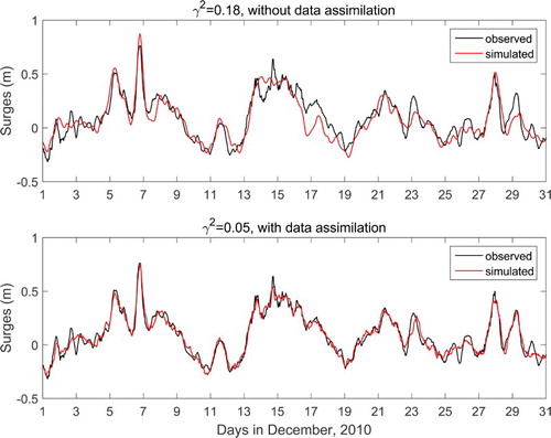
The smaller this value is, the better the fit between the simulations and the observations. The value for the non-data-assimilative solution is 0.18, which means that 82% of the observed variance is explained by the solution. The value for the assimilative solution is 0.05, so 95% of the observed variance is explained by the assimilative solution. Thus, Fig. 1 is a good illustration of the power of the ASGF regression model. We will use this model for the long-term hindcast and forecast.

In passing, we would like to note that the regression model, Eq. (2), can also be applied to a tidal problem when the atmospheric forcing in matrix is replaced by tide-generating forcing (as described in the last paragraph of Appendix A). The above procedure can then serve as a data-assimilative tidal model to give a good tidal solution, which is important because tides are dominant signals in observed sea levels. When matrix contains both atmospheric forcing and tide-generating forcing, the regression model becomes a data-assimilative model for total sea levels. However, for the scope of our paper we will focus our application on storm surges only. The application to tidal problems will be addressed in a separate paper.

3 Data-assimilative hindcast with the MERRA forcing field

We used data from MERRA for the forcing field for the short-term test case shown in Fig. 1. We will also use this forcing field for the long-term hindcast. This forcing dataset is preferable because it is highly realistic, has an hourly temporal resolution (which is high compared with other similar products), and covers the entire globe, which suits the ASGF approach. For any hour, the MERRA forcing field gives a vector of 408,622 elements consisting of the data points for air pressure and wind stress over the global ocean. Figure 2 shows the Sept-Îles storm surge hindcast results in three different ways. The simulations are shown in red and the observations in black; the period of the hindcast is from 30 July 1979 to 31 December 2011.

Fig. 2 Long-term simulations of storm surges (top) without data assimilation, (middle) with equally weighted data assimilation, and (bottom) with surge-weighted data assimilation. The simulations are shown in red and the observations are shown in black with data gaps. The data outside the yellow band are larger than 35 cm in absolute value and are referred to as surge data. The simulations are continuous but are not shown when there are data gaps.

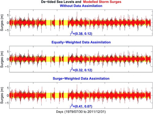
The top panel shows the simulation without data assimilation; the middle panel shows the data-assimilative simulations with all the data weighted equally, and the third panel shows the results from the weighted least-squares fit, with the surge data weighted nine times more than the non-surge data. The surge data are those that are outside the yellow band (outside ±35 cm), and these are more likely caused by storms than those within the yellow band; not all detided signals can be attributed to atmospheric forcing. There are 240,903 hourly data in the observations, of which 9318 are outside the yellow band. For simplicity in wording, we will refer to those outside the yellow band as surge data or simply surges, and those within the band will be referred to as non-surge data.

The misfit measurement is indicated in each panel with two values, the first for all misfits and the second for surge data misfits. The first and second values of indicated in the top panel are 0.38 and 0.12, respectively. This means that the simulations and observations agree much better for the surge data than for all the data. The middle panel of the figure shows the results of the data assimilation when all the data are weighted equally. The data assimilation improves the fit, but the improvement is mostly absorbed by the non-surge data: the first value of has dropped from 0.38 to 0.32, whereas the second value remains the same to the second decimal place. We particularly wish to improve the fit for the surge data because the smaller fluctuations are not of much interest. Thus, we performed a weighted least-squares fit by replacing the matrix with , where is a diagonal matrix to weight the surge data nine times more than the non-surge data. The result of this surge-weighted data assimilation is shown in the third panel. The agreement between the simulations and the surge data has improved significantly, with the value dropping from 0.12 to 0.07. However, the improvement comes at the cost of an increase in the for all misfits, the majority (96%) of which are non-surge data. This is a compromise that we can accept given our main interest.

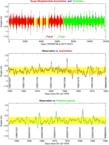
What if we reserve half the data from the data assimilation—could the model be trained with the first half of the data to provide a good prediction for the second half? Figure 3 shows the results of this investigation. The first half of the observations (about 16 years of hourly data) is assimilated with the weighting scheme mentioned above. The red curves are for the assimilative simulations, and the black curves are the observations. The green curves represent predictions for the second half of the period (about 16 years of hourly data also) by the model trained with only the first half of the observations. The value for the surges for the data assimilation half is 0.07 and that for the prediction half is also 0.07; this is satisfactory. Shown in the middle and bottom panels of the figure are two enlarged views of the assimilation half and the prediction half, respectively. The results of this investigation are encouraging; it seems valid to use the trained surge model to predict future surges using a climate model solution as the forcing field.

Fig. 3 (top) Half data assimilation and half prediction: the assimilative solution is shown in red, the prediction is shown in green, and the observations are in black. The misfit measurements (for surges only) for the assimilation and for the prediction are shown by the values in red and in green, respectively. (middle) and (bottom) Two enlarged views of the top panel.

4 Climate forecast of storm surges using the CRCM/AHJ forcing field

By climate forecast we mean a prediction of future storm surges using a climate model solution as the forcing field. The climate is stochastic. A solution output by a climate model run is just one of many possible realizations of the stochastic process. Climate model solutions are not constrained by observations, even though the model run starts in the past. We should, therefore, not expect a one-to-one correspondence between the climate model solutions and real events in the past. Storm surges driven by the climate model solutions will also be stochastic; they should not be expected to correspond to real past events either. The value of having stochastic storm surges is that they can provide a basis for statistics. The more stochastic the storm surges we can produce, the more robust the statistics.

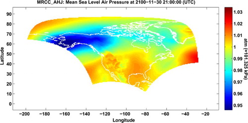
For this study, we will use the CRCM/AHJ climate model solution to provide a forcing field. The CRMC/AHJ is a regional climate model solution. Its regional coverage is outlined in Fig. 4. Its three-hourly forcing field will be interpolated to hourly because the ASGF (i.e., the matrix in Eq. (A16)) is hourly. The forcing field ranges from 0000 utc 1 January 1961 to 2100 utc 30 November 2100, so there are almost 140 years of hourly storm surges to generate. With the ASGF method, this takes less than eight seconds to generate on a personal computer.

Fig. 4 Snapshot of the mean sea level air pressures at 2100 utc 30 November 2100 using the CTRCM/AHJ solution.

To calculate storm surges for the future, we use Eq. (4) with the matrix calculated with the CRCM/AHJ forcing field (see Eq. (A33) in the Appendix) and with obtained from the surge-weighted assimilation of the 32 years of observations (Fig. 2, third panel). The forcing field is regional, whereas the ASGF matrix is prepared for the global ocean. This means that we have to assign null values for the forcing field outside the regional domain. We also subtract a standard air pressure (101.325 kPa) from the air pressure within the regional domain to avoid a large imbalance in the air pressures within the domain and outside. Subtracting a constant value from the air pressure field has no effect on the surge dynamics.

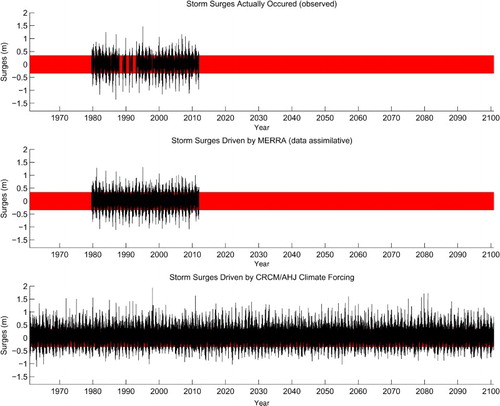
The bottom panel of Fig. 5 shows the time series of storm surges driven by the CRCM/AHJ. For reference, we also show the observations and realistic simulations with the MERRA forcing field in the same time axes in the top and middle panels, respectively. We can see that storm surges driven by the CRCM/AHJ are much stronger than the realistic ones when we compare the bottom panel with the top panel or middle panel for the same period. This indicates that the CRCM/AHJ forcing is too strong and will result in a systematic bias in the simulated future storm surges. We will correct this bias in the next section.

Fig. 5 Time series of storm surges at Sept-Îles, (top) observations, (middle) driven by the MERRA forcing field, and (bottom) driven by the CRMC/AHJ forcing field. Data points outside the red band have an absolute value larger than 35 cm. From the top to the bottom panels, the means of the time series are 0.00, 0.00, and 0.00 cm, respectively and the standard deviations are 15.91, 17.06 19.71 cm, respectively.

5 Extreme value analysis of future storm surges

The time series shown in the bottom panel of Fig. 5 can be explored statistically in many ways. The statistics we explore in this section involve applying Gumbel's extreme value analysis (EVA) to the simulated time series. In probability theory, the limiting distributions of extremes fall into one of three limiting distributions for a sequence of independent and identical parental distributions from which the extremes are drawn (e.g., Coles, 2001). Gumbel's distribution is one of the three limiting distributions and is commonly chosen to describe the extremes of water levels. According to Gumbel (1954, 1958), the return periods of annual storm surge maxima should obey a straight line distribution on a double-logarithmic scale. Shown in the left panel of Fig. 6 are such straight lines, along with the experimental data and confidence intervals, in black and blue, respectively, for the observed and simulated annual maxima from 1979 to 2011.

Fig. 6 (left) EVA results from the simulated annual maxima (blue) and from the observed annual maxima (black). The symbols are the experimental data; the straight lines are the least-squares fit lines, and the shaded intervals are the 67% confidence intervals. The results in blue are systematically biased from those in black. (right) The data and line in blue are corrected for biases.

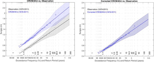
As we can see, the EVA results in blue show a systematic bias compared with those in black. This means that the CRCM/AHJ forcing field is too strong compared with reality, and we need to correct for this bias. The correction can be done by first determining the difference in the slopes and intercepts between the blue and black lines. We can then adjust the line, the data points, and the confidence interval in blue by applying the differences. The results after correction are shown in the right panel of the figure: the line and the confidence interval in blue now overlap those in black. The two sets of data points are not necessarily coincident, but they all fall along the straight line.

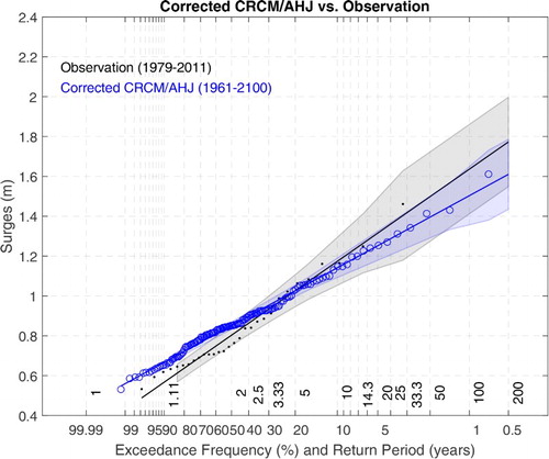
Figure 7 shows the results from applying the EVA to the 140-year hourly time series as a whole after correction for the CMCR/AHJ forcing bias. An obvious benefit from having such a long time series is that the Gumbel line is constrained by more data points, especially at the top end; there are data points beyond the 32-year return period that control the line. Consequently, the confidence interval in light blue becomes somewhat narrower than that in grey. Another noteworthy feature is that the blue line is less steep than the black line. The two lines intersect near the coordinates (5, 1), which means that the model simulation gives a longer return period than the observations for storm surges larger than 1 m. However, their associated confidence intervals still overlap.

Fig. 7 The simulated annual maxima from 1961 to 2100, the best fit Gumbel's straight line, and the associated 67% confidence interval are show in blue; the counterparts from the observed 1979–2011 annual maxima are in black.

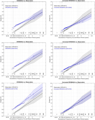
The results of applying EVA to tri-decadal sections of the time series from 2012 to 2100 are shown in Fig. 8. The tri-decadal periods are 2012–2042, 2043–2072, and 2073–2100 (the last period is two years shorter). The left panels give the results without correction for the CRCM/AHJ bias, and the right panels give the results with the correction. The EVA results from past observations (1979–2011) are superimposed on each panel for comparison. This tri-decadal approach attempts to investigate whether there is a progressive shortening or lengthening in the return periods of storm surges, which is a concern with climate change. However, by comparing the blue and black areas on the right panels, we see neither a progressive shortening nor lengthening of the return periods for the same sizes of storm surges; the bottom right panel of Fig. 8 for the 2073–2100 period shows almost the same pattern as the panel on the right of Fig. 6 for the 1979–2011 period. This comparison with the period in the past is valuable because it can indicate whether there is a tendency in the climatically simulated storm surges relative to what has actually happened.

Fig. 8 Results of the EVA applied to tri-decadal segments of the storm surges driven by CRCM/AHJ. (left) Results without bias corrections; (right) results with bias corrections.

6 Summary and discussion

We have demonstrated that the ASGF regression model can be used as an efficient tool for converting appropriate climate model solutions hydrodynamically to a database of future storm surges. The ASGF regression model is derived from a traditional storm surge model but can produce simulations orders of magnitude faster. It can easily assimilate observed data into simulations. Weighted data assimilations can also be executed easily.

For the demonstration, we used the ASGF regression model derived for Sept-Îles to first assimilate 32 years (1979–2011) of detided data, weighting large data values (>0.35 m) more than smaller values. Large data values are more likely driven by storms than smaller data values. The data assimilation produces a continuous hindcast of storm surges at Sept-Îles and yields the best-estimate regression model parameters, which can be used for a climate prediction. For the climate prediction, we used the CRCM/AHJ climate model solution to provide a forcing field from 1961 to 2100. Using the best-estimate regression parameters and with the CRCM/AHJ forcing field, the ASGF regression model produces a 140-year hourly time series of storm surges in a few seconds.

Such a time series can be used for statistical studies with various approaches. For example, our approach was to subject the time series to Gumbel's EVA. A portion of the simulated time series overlaps the observation time series (see Fig. 5), which made it possible to determine whether the simulation driven by CRCM/AHJ was statistically biased compared to reality. Indeed, we found that there is a bias and we corrected for it (see Fig. 6 and Fig. 8). Such a bias correction may also be needed when using other climate model solutions to drive storm surges. We applied EVA to the 140-year time series as a whole, as well as to tri-decadal segments. The tri-decadal approach was an attempt to investigate whether there was any progressive shortening of the return periods of the storm surges, but our investigation does not reveal this to be the case.

We do not wish to interpret the above EVA results as a general conclusion because they are based on only one of many possible climate forcing fields. The main point of this study is to demonstrate that the ASGF regression model shown in Eq. (2) can be used as an efficient tool for converting a long-term climate model solution to a storm surge time series of the same length at a particular POI. The procedure shown by this demonstration can be repeated for other POIs and with other climate forcing fields. As more climate model solutions are collected for this purpose, a larger database of future storm surges can be established, and more robust statistics can be drawn upon. A project is currently underway to apply the same procedure to the permanent tidal gauges operated by the Canadian Hydrographic Service.

Acknowledgements

The CRCM data were generated and supplied by Ouranos. NASA's free access to MERRA data is also greatly appreciated. The authors acknowledge support from their institutes and express thanks to Mr. Michel Beaulieu for his assistance. We also thank two anonymous reviewers for their constructive comments and Ms. Laure Devine for her proofreading and editing.

Funding

This study was partially supported by le Ministère des Transports du Québec and by the Aquatic Climate Change Adaptation Services Program (ACCASP) program of Fisheries and Oceans Canada.

Disclosure statement

No potential conflict of interest was reported by the authors.

Notes

^†A wind and wave hindscast dataset for the first 40 years (1958-1997) produced by the Meteorological Service of Canada (formerly the Atmospheric Environment Service (AES).

Appendix A: From a traditional storm surge model to an ASGF regression model

We chose the following linear and depth-averaged shallow water equations to govern storm surges; written in matrix form, they are(A1)

where t is the time variable; x and y are the arc lengths along circles of latitude and longitude related to longitude λ, latitude ϕ, and the Earth's mean radius R (taken as 6371 km) by x = Rλ cosϕ, and y = Rϕ; , and ; η, u, and v are the sea-surface elevation and the mass fluxes in the longitudinal and latitudinal directions, respectively; f and g are the Coriolis parameter and acceleration due to gravity, respectively; and h and κ are the water depth and bottom friction coefficient, respectively. Note that the partial operator in the matrix affects all the factors to its right (e.g., the multiplication of by v should be understood as ). To avoid the polar singularity, a rotated spherical coordinate system is used, the pole of which is rotated to (40°W, 80°N), a point in Greenland.

The second term of the right-hand side of Eq. (A1) contains the forces of atmospheric pressures and wind stresses. The air pressures at mean sea level, , enter into the momentum equation as the inverse barometer :(A2)

where is seawater density, taken as 1025 kg m⁻³. The wind stresses and are obtained by converting the wind velocity components, and , at 10 m above sea level with(A3)

where refers to the air density, taken as 1.25 kg m⁻³, and is the drag coefficient specified by(A4) The formula for the drag coefficient was modified from Csanady (1982). The second line of the above equation is the trial and error modification to fit our model solutions to an observed storm surge.

At the sea bottom, a linear frictional stress, , is used (following Heaps, 1969). However, Heaps used the constant κ = 0.0024 m s⁻¹, whereas here a spatially varying is adopted following Ding, Jia, and Wang (2004) and Tan (1992) such that it is inversely proportional to the cubic root of water depth. This results in κ ranging from 4.5 × 10⁻⁴m s⁻¹ to 4.6. × 10⁻³m s⁻¹ in the world ocean. This is an attempt to reflect a general fact that there is less bottom friction in deep water than in shallow water. For further details, see Xu (2011).

The world ocean is taken as the model domain and the General Bathymetric Chart of the Ocean (GEBCO08; http://www.gebco.net) is used for the model's bathymetry. An advantage of using the global ocean as the model domain is that the model is free of artificial open-water boundaries: all the lateral boundary conditions are zero normal flow conditions to the true coasts, that is,(A5) (A6)

When discretized with a valid difference scheme, the linear dynamic system of Eqs (A1) to (A6) can always be expressed as(A7)

where k is a zero-based time stepping index and the bold letters are the discretized versions of their continuous counterparts in Eq. (A1). The matrix updates the state vector from the current time step to the next. The initial value of the state vector can be assumed to be zero for the storm surge problem. The matrix maps the atmospheric forcing into momentum to change the state vector with time.

Introducing to denote the state vector and f to denote the forcing vector , then(A8)

Therefore, we can present Eq. (A7) in a compact form,(A9) (A10) where the superscripts with parentheses refer to time steps. The initial value of the state vector, , is assumed to be zero. This is justified because the effect of any non-zero initial condition will become negligibly small after the ocean is fully spun up by external forcing.

The solution to Eqs (A9) and (A10) is(A11)

where is the ith power of matrix . Assuming that we are only interested in the nth component of the state vector x(n), which represents the sea surface elevation η at a POI (i.e., let η = x(n) be of interest) then from the above we have(A12)

where is nth row of the ith power of the matrix , that is,(A13)

where the : symbol represents all the columns ranging successively from 1. To obtain , we do not need to calculate the ith power of the entire matrix ; it can be calculated economically using the following iterations:(A14) (A15) Each iteration involves only the multiplication of a row vector by a matrix, which is very computationally efficient. Xu (2015b) showed that a proper value for is such that , where Δt is the time step associated with the storm surge model Eq. (A1).

Collect all the vectors into another matrix ,(A16)

With this , we can rewrite Eq. (A11) concisely as(A17)

where is a vector of time series and the sign * means a convolution operator defined as(A18)

The matrix defines the ASGF. The rows of are domains of dependence of the solutions at the POI at different times. The columns of are the Green's functions to the impulses placed at different grid points. There are as many columns as the total number of grid points, and all grid points are allowed to be potential source points, as implied by the name “all-source” Green's functions. Xu (2015a) interprets the matrix in more detail and discusses how to reduce the dimensions of the matrix according to the temporal and spatial resolutions of a given forcing field.

Applying SVD to we obtain(A19) and substituting the decomposition into Eq. (A17) we obtain(A20)

It can be proven that the operator * can be moved between and , that is, the following relationship is true (see Xu, 2015b)(A21)

Thus, Eq. (A17) can be further transformed as(A22)

where(A23)

is a compressed forcing field.

It can be proven that(A24)

where is a column vector consisting of the diagonal elements of the matrix in Eq. (A19); is the jth column of ; and is a column vector consisting of the time series of ψ_j, with j = 1,2, … , m. For simplicity, to prove this without loss of generality, let us assume that the dimensions of and are 2 × 2:(A25)

and that the forcing field consists of only two instantaneous vectors, and ,(A26) In this simple case,(A27) (A28) (A29) (A30)

where and stand for the first and second columns of ;  and are defined by(A31) They are vectors in time whereas those defined in Eq. (A26) are vectors in space. The same procedure revealed by this simple example may be used to prove Eq. (A24) by the mathematical induction method.

Substituting the above into Eq. (A22) gives us(A32)

where is a matrix, defined as(A33)

By including an error term, Eq. (A32) becomes(A34) where ε is an error vector consisting of the errors of the observations, of the forcing field, and of the model itself. The parameter vector s can now be relaxed from the given values to be determined by a least-squares fit between the model and the observations.

Thus, a traditional storm surge model represented by Eqs (A9) and (A10) has been simplified to the regression model in Eq. (A34). This ASGF regression model can not only yield data-assimilative solutions but can also run orders of magnitude faster than the traditional model, as reported by Xu (2015b).

It is worthwhile noting here that if we replace η_a with the tide-generating potential and we set the wind stresses τ_x and τ_y in Eqs (A7) and (A8) to zero, then what is considered in this Appendix becomes a tidal problem and the end result, Eq. (A34), is a data-assimilative tidal model for the tides at a POI driven by the global tide-generating forcing.

References

- Bernier, N. B., & Thompson, K. R. (2006). Predicting the frequency of storm surges and extreme sea levels in the northwest Atlantic. Journal of Geophysical Research: Oceans (1978–2012), 111, C10009, 1–15. doi:10.1029/2005JC003168
- Coles, S. (2001). An introduction to statistical modeling of extreme values. London: Springer.
- Csanady, G. T. (1982). Circulation in the coastal ocean. Dordrecht: Reidel.
- Ding, Y., Jia, Y., & Wang, S. S. (2004). Identification of Manning's roughness coefficients in shallow water flows. Journal of Hydraulic Engineering, 130(6), 501–510. doi: 10.1061/(ASCE)0733-9429(2004)130:6(501)
- Gumbel, E. J. (1954). Statistical theory of extreme value and some practical applications. Applied Mathematics Series No. 33 (1st ed.). U.S. Department of Commerce, National Bureau of Standards. ASIN B0007DSHG4.
- Gumbel, E. J. (1958). Statistics of extremes. New York: Columbia Univ. Press.
- Heaps, N. S. (1969). A two-dimensional numerical sea model. Philosophical Transactions for the Royal Society of London. Series A, Mathematical and Physical Sciences, 265(1160), 93–137. doi: 10.1098/rsta.1969.0041
- Jungclaus, J. H., Keenlyside, N., Botzet, M., Haak, H., Luo, J. J., Latif, M., … Roeckner, E. (2006). Ocean circulation and tropical variability in the coupled model ECHAM5/MPI-OM. Journal of Climate, 19(16), 3952–3972. doi: 10.1175/JCLI3827.1
- Music, B., & Caya, D. (2007). Evaluation of the hydrological cycle over the Mississippi River basin as simulated by the Canadian Regional Climate Model (CRCM). Journal of Hydrometeorology, 8(5), 969–988. doi: 10.1175/JHM627.1
- Nakićenović, N., & Swart, R. (Eds) (2000). Special report on emissions scenarios. ISBN 0521804930. Cambridge, UK: Cambridge University Press.
- Ouranos Consortium. (2012). Tri-decadal A2 CRCM4-CGCM3 and CRCM4-ECHAM5 fields on AMNO 45-km grid. Final report for contract No. F5957–120148 for the Ocean Circulation Section of the Bedford Institute of Oceanography. Retrieved from ftp://www2.mar.dfo-mpo.gc.ca/pub/ocean/ACCASP%20Trends%20&%20Projections/Ouranos%20AMNO/Ouranos_DFO_20July2012_v_final.pdf
- Roeckner, E., Bäuml, G., Bonaventura, L., Brokopf, R., Esch, M., Giorgetta, M., … Tompkins, A. (2003). The atmospheric general circulation model ECHAM 5. Part I: Model description. Max Planck Institute for Meteorology. Report No. 349. Retrieved from http://www.mpimet.mpg.de/fileadmin/publikationen/Reports/max_scirep_349.pdf
- Seber, G. A., & Lee, A. J. (2003). Linear regression analysis. Hoboken, New Jersey: John Wiley & Sons, Inc.
- Strang, G. (1986). Introduction to applied mathematics. Wellesley, MA: Wellesley-Cambridge Press.
- Strang, G. (2007). Computational science and engineering. Wellesley: Wellesley-Cambridge Press.
- Swail, V. R., Ceccacci, E. A., & Cox, A. T. (2000). The AES40 North Atlantic wave reanalysis: Validation and climate assessment. In 6th International Workshop on Wave Hindcasting and Forecasting November (pp. 6–10).
- Swail, V. R., & Cox, A. T. (2000). On the use of NCEP-NCAR reanalysis surface marine wind fields for a long-term North Atlantic wave hindcast. Journal of Atmospheric and Oceanic Technology, 17, 532–545. doi: 10.1175/1520-0426(2000)017<0532:OTUONN>2.0.CO;2
- Tan, W. Y. (1992). Shallow water hydrodynamics: Mathematical theory and numerical solution for a two-dimensional system of shallow-water equations. Amsterdam: Elsevier.
- Xu, Z. (2007). The all-source Green's function and its applications to tsunami problems. Science of Tsunami Hazards, 26(1), 59–69.
- Xu, Z. (2011). The all-source Green's function of linear shallow water dynamic system: Its numerical constructions and applications to tsunami problems. In Nils-Axel Mörner (Ed.), The tsunami threat – Research and technology, Rijeka InTech, Retrieved from http://www.intechopen.com/books/the-tsunami-threat-research-and-technology/the-all-source-green-s-function-of-linear-shallow-water-dynamic-system-its-numerical-constructions-a doi:10.5772/14062
- Xu Z. (2015a) The All-Source Green’s Function (ASGF) and its applications to storm surge modelling. Part I: From the governing equations to the ASGF convolution. Ocean Dynamics. in press. doi:10.1007/s10236-015-0893-z
- Xu Z. (2015b) The All-Source Green’s Function (ASGF) and its applications to storm surge modelling. Part II: From the ASGF convolution to forcing data compression and to a regression model. Ocean Dynamics. in press. doi:10.1007/s10236-015-0894-y
- Xu, Z., & Song, Y. T. (2013). Combining the all-source Green's functions and the GPS-derived source functions for fast tsunami predictions–Illustrated by the March 2011 Japan Tsunami. Journal of Atmospheric and Oceanic Technology, 30(7), 1542–1554. doi: 10.1175/JTECH-D-12-00201.1