Large-Scale Atmospheric and Oceanic Control on Krill Transport into the St. Lawrence Estuary Evidenced with Three-Dimensional Numerical Modelling

ABSTRACT

A three-dimensional circulation model, coupled to a Lagrangian particle drift model, is used to understand the processes leading to krill transport from the northwest Gulf of St. Lawrence (nwGSL) towards the head of the Lower St. Lawrence Estuary (LSLE), a well-known site of krill accumulation. An analysis of the circulation at the scale of the Gulf of St. Lawrence (GSL) over five years (2006 to 2010) evidenced four major findings. (i) There are two main seasonal circulation patterns, one in winter–spring and one in summer–fall, driven by local wind forcing and transport at Cabot Strait and at the Strait of Belle Isle. (ii) The freshwater runoff variability does not control the observed inflow events at the mouth of the LSLE. (iii) Extratropical storms passing over the GSL are important for the transport of krill into the LSLE through the generation of inflow events at Pointe-des-Monts. (iv) The contribution of the transport in the surface layer (where krill are found at night) during these inflow events is also important in modulating the variability of the transport of krill into the LSLE. The inflow events, combined with the presence or absence of high krill densities in the nwGSL, partly control the interannual variability of the transport of krill into the LSLE.

RÉSUMÉ

[Traduit par la redaction] Nous utilisons un modèle tridimensionnel de circulation, couplé à un modèle lagrangien de dérive de particules, afin de comprendre les processus menant au transport du krill, du nord-ouest du golfe du Saint-Laurent vers la tête de l'estuaire maritime du Saint-Laurent, un site bien connu d'accumulation de krill. Une analyse de cinq ans (2006 à 2010) de la circulation, menée à l’échelle du golfe du Saint-Laurent, a conduit à quatre découvertes majeures : (i) il existe deux configurations saisonnières principales de circulation, une présente en hiver et au printemps, et une autre en été et en automne, quisont contrôlées par le forçage local du vent, et le transport dans les détroits de Cabot et de Belle Isle; (ii) la variabilité du débit d'eau douce ne régit pas les évènements d'entrée d'eau à l'embouchure de l'estuaire maritime du Saint-Laurent; (iii) les tempêtes extratropicales qui passent au-dessus du golfe du Saint-Laurent s'avèrent importantes pour le transport du krill vers l'estuaire maritime du Saint-Laurent, en raison de la génération d'évènements d'entrée d'eau à Pointe-des-Monts; (iv) la contribution du transport dans la couche de surface (où le krill se trouve la nuit), qui module la variabilité du transport du krill dans l'estuaire maritime du Saint-Laurent durant ces évènements d'entrée d'eau, revêt aussi de l'importance. Les évènements d'entrée d'eau, combinés à la présence ou à l'absence de densités élevées de krill dans le nord-ouest du golf du Saint-Laurent, régissent partiellement la variabilité interannuelle du transport du krill dans l'estuaire maritime du Saint-Laurent.

KEYWORDS:

• marginal seas
• biophysical interactions
• circulation
• seasonal cycle
• modelling
• zooplankton aggregation
• diel vertical migration

1 Introduction

This study is part of an Ecosystem Research Initiative (ERI) led by the Canadian Department of Fisheries and Oceans (Gagné et al., 2013) that targeted the Lower St. Lawrence Estuary (LSLE; between the Saguenay Fjord and Pointe-des-Monts (PdM)). The LSLE is a biologically productive area where large krill aggregations are found, especially in the Saguenay–St. Lawrence Marine Park at the head of the Laurentian Channel (Simard, de Ladurantaye, & Therriault, 1986; Simard & Lavoie, 1999). These aggregations are exploited by marine mammals and fish that feed on them. One of the goals of the ERI was to study the ecological and oceanographic processes determining the presence of pelagic forage species and rorqual whales (blue, fin, etc.) frequenting the LSLE on a seasonal basis.

The hydrodynamic circulation in the Gulf of St. Lawrence (GSL) is generally cyclonic, and two of its main oceanographic features are the Gaspé Current and the Anticosti Gyre (Fig. 1). The GSL is connected to the Atlantic Ocean through two openings: the shallow (less than 60 m) and narrow (15 km) Strait of Belle Isle (hereafter SBI) and the deeper (480 m) and wider (104 km) Cabot Strait (Fig. 1). The transport at SBI, combined with the freshwater outflow of the LSLE, is thought to be important for the maintenance and strength of the Anticosti Gyre and Gaspé Current (Sheng, 2001), while the transport at Cabot Strait has a major influence on the water levels in the GSL (Bobanovic & Thompson, 2001). Wind forcing is also an important source of kinetic energy in the GSL (Koutitonsky & Bugden, 1991). In general, wind velocities are higher in winter than in summer and frequently blow from the northwest in winter (Drinkwater & Pettipas, 1993). The GSL bathymetry is characterized by deep channels that carry waters from the Atlantic Ocean far inland. In particular, the 300–540 m deep Laurentian Channel extends over about 1250 km from its mouth at the continental slope to its head at the Saguenay Fjord confluence, where the bottom shoals rapidly and where tidal upwelling and mixing enhance the estuarine circulation. The GSL has two layers in winter: a near-freezing surface mixed layer and a deep layer of oceanic origin. At the end of spring, increased freshwater runoff, sea-ice melt, and insolation combine to form a buoyant surface layer that isolates the winter surface layer which in turn forms the cold intermediate layer (CIL). The CIL is then advected upstream towards the head of the Laurentian Channel and slowly warms until the following fall when wind mixing and surface cooling cause the surface layer to merge with the CIL again (Galbraith, 2006; Gilbert & Pettigrew, 1997).

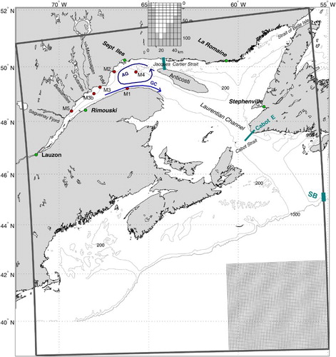
Fig. 1 Map of the study area showing the model domain, with a small sub-area of the grid in the lower right corner. The 200 and 1000 m depth contours are shown. The blue arrows represent the position of the Anticosti Gyre (AG) and Gaspé Current (GC). The red dots show the locations of the five ADCP moorings (M1, M2, M3 (and its relocated position M3b), M4, and M5). The thick blue line shows the position of the Jacques-Cartier Strait transect (see inset for the model depths across the transect from the south towards the north). The thick blue line at the shelf break south of Newfoundland shows the location of the SB valve (i.e., where the shelf break transport was modified for the Cabot Strait transport sensitivity analysis). The eastern half of the Cabot Strait transect (Cabot-E) is also depicted with a blue line.

One peculiarity of the krill population found in the LSLE is that it is mostly composed of older stages of the two dominant species: Thysanoessa raschi and Meganyctiphanes norvegica (Simard & Lavoie, 1999). Younger stages are found downstream in the GSL (Berkes, 1976). Both species perform diel vertical migration (DVM), occupying similar depths when at the surface (0–50 m) at night, but T. raschi is generally found above M. norvegica during the day (e.g., Berkes, 1976; Harvey, Galbraith, & Descroix, 2009). The daytime depth of these two species is in great part related to light levels in the water column and thus varies spatially and temporally (Plourde et al., 2013). Simard and Lavoie (1999) hypothesized that a sorting mechanism would be at play: adults, which spend more time at depth, would be advected upstream from the GSL by the two-layer estuarine circulation, while the younger stages, which spend more time at the surface, would be carried downstream. It is not clear what fraction of krill advected downstream eventually returns to the northwest Gulf of St. Lawrence (nwGSL) and what fraction is eaten downstream by predators in the shallower southern GSL (Simard & Harvey, 2010), or flushed out of the GSL (e.g., Sameoto and Herman (1992) for copepods). However, it is well accepted that the nwGSL is the source of krill for the LSLE and that krill enter the LSLE principally along the north shore (Simard, 2009).

Sourisseau, Simard, and Saucier (2006) tried to reproduce the observed seasonal distribution of krill in the LSLE and GSL using a three-dimensional (3D) sea-ice–ocean circulation model coupled to a krill biomass-concentration equation with an active DVM. Their results showed aggregations forming in the LSLE when particles remained at depth at all times, demonstrating the importance of upstream advection of krill while at their daytime depth. However, they failed to reproduce aggregations in the LSLE when the organisms were undergoing DVM. Some processes were thus missing in their model, either in the krill DVM (Sourisseau, Simard, & Saucier, 2008) or 3D circulation (Saucier, Roy, Gilbert, Pellerin, & Ritchie, 2003) models. Various processes that could influence the circulation at the mouth of the estuary were discussed but the actual mechanisms responsible for the large inflow of vertically migrating krill at PdM were not established.

The circulation at the mouth of the LSLE is indeed complex. Numerous studies showed the importance of meteorological forcing within the LSLE and on the variability of the exchanges between the GSL and the LSLE (e.g., Mertz, El-Sabh, & Koutitonsky, 1988; Mertz, Koutitonsky, Gratton, & El-Sabh, 1992; Tee, 1989). Meteorological forcing generates oscillations in the current and salinity fields with periods of 10–15 and 40–50 days in the LSLE and would be the dominant source of synoptic variability at the mouth of the LSLE (Mertz et al., 1988). Seasonal time-scale variations in the surface current field of the LSLE were also observed and attributed to the runoff cycle of the St. Lawrence River (Koutitonsky, Wilson, & El-Sabh, 1990; Mertz, El-Sabh, & Koutitonsky, 1989). The freshwater runoff from the St. Lawrence River and the Saguenay Fjord drives a surface outflow that forms a jet along the south shore of the estuary downstream of the Saguenay Fjord. This jet can remain along the south shore as far as the tip of the Gaspé Peninsula, but it sometimes bifurcates towards the north shore near Rimouski to form a north shore jet. This jet detaches from the shore near PdM, crossing the mouth of the LSLE and reinforces the Gaspé Current (e.g., Koutitonsky and Bugden (1991) and references therein). Depending on these circulation patterns, an anticyclonic or a cyclonic eddy can be found between Rimouski and the mouth of the LSLE. A shift between these two regimes in July 1979 was observed by Mertz et al. (1989) and Koutitonsky et al. (1990).

In order to properly simulate the transport of migrating krill in this hydrodynamically complex environment, currents were measured at five stations specifically located to validate the simulated LSLE and nwGSL circulation obtained with our 3D ocean circulation model (Fig. 1). A Lagrangian particle-tracking model was then coupled to the 3D circulation model to investigate the physical processes leading to the transport of krill from the nwGSL and up the LSLE. This study has similar goals to those of Sourisseau et al. (2006), but we used a different hydrodynamic model, also eddy resolving, that allows inflow of surface and sub-surface water along the north shore of the LSLE and a refined krill DVM model based on extensive in situ observations. We used a particle-tracking model to avoid the conservation problems inherent with advection-diffusion in Eulerian models (Campin, Adcroft, Hill, & Marshall, 2004) and a photoperiod-responding krill DVM model and daytime and nighttime vertical distributions based on year-round acoustic in situ observations at the same stations where currents were measured. A companion study by Maps, Plourde, Lavoie, McQuinn, and Chassé (2013) looked at the influence of differences in the daytime depth of the two main krill species on their transport across three specific transects in the GSL. Our goal is to identify the processes that lead to major inflow of krill from the nwGSL towards the LSLE on a seasonal basis.

2 Methods

a Ocean Circulation Model

The ocean circulation model used in our study is based on the Nucleus for European Modelling of the Ocean (NEMO) system, which is described in detail in Brickman and Drozdowski (2012). The modelling system is based on the Océan PArallélisé code, version 9.0 (OPA; Madec, 2012). A thermodynamic-dynamic sub-model, Louvain-la-Neuve Sea Ice Model (LIM2; Goosse & Fichefet, 1999; Madec, Delecluse, Imbard, & Lévy, 1998), is coupled to the circulation model. The grid of the model covers the GSL, the Scotian Shelf, and the Gulf of Maine (Fig. 1). The grid has a horizontal resolution of 1/12° in latitude and longitude (about 6 × 8 km depending on the location) and 46 layers of variable thickness (from 6 m close to the surface to 250 m at depth in the ocean). The first 19 layers cover all depths of the GSL (maximum depth of ∼540 m). It is a prognostic model, meaning that the temperature and salinity fields are free to evolve with time and are only constrained through open boundary conditions, freshwater runoff, and surface forcing. Monthly temperature and salinity climatologies, built from extensive Fisheries and Oceans Canada databases over the 1971–2000 period, are used to initialize the model and set the open boundary conditions. An annual cycle of the barotropic transport is prescribed at the SBI in addition to a smaller baroclinic transport calculated from the monthly temperature and salinity fields. Five tidal components (M₂, S₂, N₂, O₁, K₁) are included in the model through surface elevation and transports at the open boundaries. Freshwater enters the domain through precipitation and runoff from the 78 main rivers. The monthly runoff of the St. Lawrence River is estimated from sea level measurements at Lauzon using the approach of Bourgault and Koutitonsky (1999) and obtained from the St. Lawrence Global Observatory (http://ogsl.ca/en.html). Runoff for all other rivers is obtained from a simple hydrological model described in Lambert et al. (2013). The hydrological model provides natural runoff curves (i.e., following precipitation and evaporation). However, the runoff from the Saguenay, Manicouagan, Betsiamites and Outardes rivers is heavily regulated by the presence of large hydroelectric dams. To reproduce the regulation effect on the runoff of these rivers, we calculated the proportion of the annual runoff released at the dams for each month of the year based on measurements made between 1970 and 2000. We then redistributed the annual runoff calculated by the hydrological model according to these proportions for each river. Three-hourly surface forcing data for the ice–ocean model (air temperature, relative humidity, winds, cloud cover, and precipitation) were obtained from the Canadian Meteorological Centre-Global Environmental Multiscale (CMC-GEM) atmospheric model (Pellerin, Lefaivre, Houtekamer, & Girard, 2003). The vertical mixing coefficient was multiplied by six in parts of the shallow Upper St. Lawrence Estuary to account for mixing processes not resolved by the model (as suggested by Saucier et al. (2003)).

b ADCP Moorings and Acoustic Backscatter

Mooring positions were chosen to validate the cyclonic circulation in the nwGSL (M1, M2, M4) and the inflow along the north shore (M3) and up the LSLE (M5) (Fig. 1). The moorings were first deployed at the end of October 2007. The instruments were retrieved in June 2008 for maintenance and redeployed in August or October 2008 until early November 2009. Mooring M3 was relocated to M3b in June 2009 after it was accidentally dragged by a fishing vessel. Each mooring had an upward-pointing 300 kHz acoustic Doppler current profiler (ADCP Sentinel, Teledyne RDI, http://www.rdinstruments.com/sen.aspx) at a depth of about 110 m and measured currents in 4 m bins up to 10 m from the surface. At station M4, an additional ADCP, pointing downward, was installed just below the upward-pointing ADCP to measure currents down to about 220 m. The raw acoustic backscatter from the ADCPs was converted to volume backscattering strength (S_v; in dB re 1 m⁻¹) following Deines (1999), providing an index of macro-zooplankton density, especially krill, and tracking their DVM (e.g., Sourisseau et al., 2008) and their relative distributions over the water column (Fig. 2).

Fig. 2 Typical mean krill nighttime and daytime vertical distribution observed with the ADCP at station M4 in July 2009. The light grey line shows a modified daytime vertical distribution to simulate aggregation of krill near the bottom in areas shallower than 100 m.

c Particle-Tracking Model

The particle-tracking module originally developed for lobster larvae by Chassé and Miller (2010) is used to follow krill within the domain. Particles are initially released uniformly over the GSL domain (400 particles per grid cell) with boundaries at Cabot Strait and SBI. Each trajectory is calculated using the common Runge-Kutta method (e.g., Butcher, 2003) with a predictor–corrector scheme. The nighttime and daytime vertical distributions of krill were determined from the ADCP backscatter (Fig. 2). The particles are redistributed from one vertical distribution to the other one hour before sunrise or sunset to mimic the civil twilight-triggered krill DVM ascent and descent. The vertical position of an individual particle within the specified daytime or nighttime profile is determined randomly. Sunrise and sunset times were calculated according to the National Oceanic and Atmospheric Administration (NOAA) solar calculator (http://www.esrl.noaa.gov/gmd/grad/solcalc/calcdetails.html) at a location (69.3°W, 48.5°N) corresponding to station M5 (Fig. 1). The vertical distribution in areas shallower than 226 m is compressed in proportion to the water column depth. In areas shallower than 100 m, the daytime vertical distribution profile was truncated at 175 m before being compressed (see light grey line in Fig. 2 for resulting distribution for a depth of 100 m) to reproduce the krill tendency of accumulating close to the bottom along shelf breaks and over shallows during daytime (e.g., Cotté & Simard, 2005; Fig. 8a in Lavoie, Simard, & Saucier, 2000). The particles are transported by the horizontal currents and are not affected by the vertical currents (only active migration generates vertical particle movement), permitting aggregation to occur with horizontal convergence.

At SBI and Cabot Strait, the particles are allowed to leave the domain with outflowing currents. New particles are created and transported into the GSL with inflowing currents so that the concentration at the boundaries is always 200 particles per grid cell (inflowing number of particles is not dependent on number of outflowing particles). The inflowing number of particles is smaller than the initial conditions to account for the fact that more krill are advected out of the GSL than into the GSL. Little is known about krill import into the GSL (quantity, seasonality, etc.) but, from a multi-year simulation (2006 to 2010), we found that some particle inflow was required to maintain the simulated amount of particles at a reasonable level over the five years.

d Simulations Description

The circulation model is spun up from rest, starting 1 May 2005, and evolves in time purely on the basis of the external forcing described above, with no restoring conditions until December 2010. This simulation will hereafter be called the Control run. Daily average currents for each grid cell are output and used thereafter in offline mode by the particle-tracking model. Five one-year simulations (one for each year between 2006 and 2010) were performed with the krill model using the hourly currents interpolated from the daily averages produced by the circulation model. The simulations were launched 1 December of the previous year to allow the particles to form aggregations along shelf breaks. To better understand the importance of the vertical distribution of krill in the system, three types of simulation were performed with (i) particles migrating between the daytime and nighttime distribution at sunset and sunrise as described in Section 2c (MIGR), (ii) particles maintaining the daytime distribution (DAY), or (iii) the nighttime distribution (NIGHT) at all times (Fig. 2). We also performed a five-year simulation to make sure that our set-up (initiation in December, number of particles per cell) did not influence our results and conclusions.

Different sensitivity analyses were also performed to determine the importance of freshwater runoff, wind forcing, and transport at the bounding straits on the processes controlling the inflow of krill in the LSLE.

1 SMOBSLcst

In this simulation, the runoff from the main rivers flowing into the St. Lawrence Estuary (St. Lawrence, Saguenay, Manicouagan, Betsiamites, and Outardes rivers) was set to their annual mean (i.e., constant runoff at all times; 10,908, 1492, 933, 344, and 381 m³ s⁻¹, respectively).

2 LowBI

The annual barotropic transport at SBI is obtained using a sinusoidal function that fits the summer and winter transport calculated by Petrie, Toulany, and Garrett (1988). In this simulation, the mean and amplitude of this sinusoidal function is reduced to obtain a small, relatively constant, transport over the year.

3 HighSB

The transport on the northern side of Cabot Strait is controlled in part by the shelf break current south of Newfoundland (SB in Fig. 1). Similar to SBI, a barotropic transport perturbation (see Brickman & Drozdowski, 2012) was added to the mean currents at SB. In this simulation, we increased the open boundary inflow along the eastern boundary at SB by doubling the mean of the sinusoidal function, from 1.5 (in the Control simulation) to 3.0. These changes then propagate to Cabot Strait, although in a non-linear fashion.

4 SWwind

To evaluate the impact of wind forcing variability on the inflow events and circulation regimes described in our paper, we made a simulation in which the wind stress components were kept positive at all times (i.e., blowing from the southwest at all times). The magnitude of the winds, however, was not modified.

3 Model performance in simulating the hydrographic conditions in the GSL

a Circulation

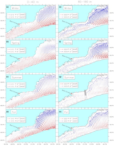
The simulated currents were averaged by season and over two different layers that correspond to the layers where most of the krill are found during night (0–40 m) and day (80–180 m, Fig. 2). Recurrent seasonal patterns were obvious for the five years simulated and are presented as a five-year mean of the simulated currents (Fig. 3). The model reproduces the known GSL circulation features, such as the Anticosti Gyre in the nwGSL, the Gaspé Current and the southeastward flow along the Magdalen Shallows (e.g., Koutitonsky & Bugden, 1991; Urrego-Blanco & Sheng, 2014b). Our mean fall and winter currents in the 0–40 m layer (Figs 3a and 3d) are very similar to the mean 0–30 m currents obtained by Urrego-Blanco and Sheng (2014a; see their Fig. 8). As the latter authors mention, there are very few measurements of currents for comparison. However, our mooring arrays allow us to validate the circulation in the nwGSL and along the north shore of the LSLE. We compared the ADCP measured currents with the simulated currents at the closest grid cell to each mooring site (Fig. 4). Both observed and simulated currents were averaged over two layers, 10–40 m and 40–100 m for observations and 6–37 m and 37–103 m for simulations, and over 24 hours. The current coordinate system (u and v) was rotated to lie in the direction of the main flow (alongshore).

Fig. 3 Mean 2006–2010 currents averaged over krill mean nighttime ((a) to (d) 0–40 m) and daytime ((e) to (h) 80–180 m) depths for each season. Blue arrows indicate westward-flowing currents and red arrows eastward-flowing currents.

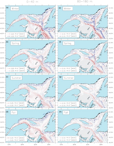
Fig. 4 Comparison of observed (blue) and simulated (red) daily mean currents over two layers, 10–40 m and 40–100 m, at stations M1, M2, M3, and M3b shown in Fig. 1. The current coordinate system was rotated by 15° to match the alongshore axis at M1, by 60° at M2, by 10° at M3, and by 30° at M3b (positive values indicate an eastward flow out except for M2 where they indicate a northward flow). The x-axis shows the time from October 2007 to November 2009. The greyed areas correspond to the events described in Fig. 13. The γ² values calculated by Eq. (1) are also displayed in the upper left corner of each panel.

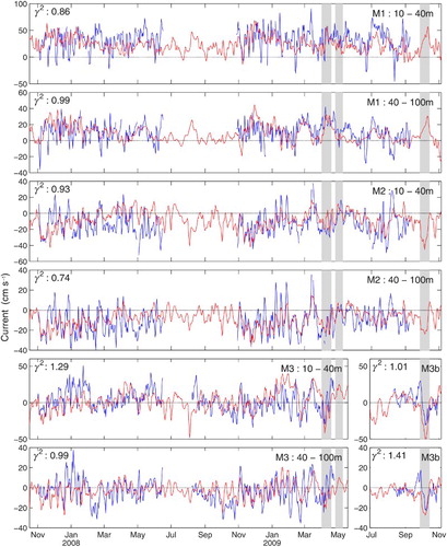
The observed and simulated currents compare well in general although there is less energy and variability in the simulated currents (i.e., the amplitudes of the oscillations are sometimes smaller in the simulated currents, which translates into weaker currents rather than current reversals). A variance discrepancy is expected with such comparisons on velocity estimates computed on different unit volumes (i.e., sample support, Chiles & Delfiner, 2012). However, most observed current reversals (from positive to negative currents and vice versa) at stations M2 and M3 are well simulated by the model. These two stations are the ones that best monitor the alongshore flow in the nwGSL and the inflow events into the LSLE.

To quantify the error we looked at the mean velocity differences for the three stations depicted (M1, M2, and M3), which are 14 cm s⁻¹ for the 10–40 m layer and 9 cm s⁻¹ for the 40–100 m layer, and we also calculated the ratio of the simulated error variance to the observed variance (γ²) as in Ohashi and Sheng (2013):(1)

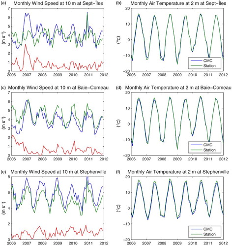
where O and M denote the observed and simulated values, respectively. The results for the entire series are displayed in each panel of Fig. 4. Using only the 2008–2009 portion of the observations, we see a reduction in the errors at M1 and M2, with γ² equal to 0.73 and 0.66, respectively, in the 10–40 m layer and 0.95 and 0.59, respectively, in the 40–100 m layer. Contrary to M1 and M2, the agreement between the simulated and observed currents at M3 does not improve during the second mooring period (2008–2009). We attribute this difference, in part, to discrepancies between the winds simulated by GEM and used as forcing and the observed winds. At Sept-Îles, a station representative of the wind forcing over the nwGSL, the difference between the observed and simulated winds is greater during the 2006–2008 period than afterwards, which could explain the lower fit between observed and simulated currents during that period (Fig. 5a). As we will see later, the interannual variability in the forcing at the model boundaries, not included in these simulations, could also contribute to the differences between the observed and simulated currents.

Fig. 5 GEM-simulated (blue line) versus observed (green line) monthly mean winds at 10 m at (a) Sept-Îles, (c) Baie-Comeau, and (e) Stephenville and (b), (d), and (f) air temperature at 2 m at the same locations. The red line on (a), (c), and (e) represents the absolute difference between observed and simulated winds. The location of the stations is displayed in Fig. 1, except for Baie-Comeau, which is displayed in Fig. 10. Wind and air temperature data were obtained from Environment Canada.

b Transport at Cabot Strait

The seasonal mean temperatures and velocities at Cabot Strait are shown in Fig. 6 for comparison with those simulated by Urrego-Blanco and Sheng (2014b) and Han, Loder, and Smith (1999). Very few in situ transport estimates are available for Cabot Strait. Our transport estimates across the eastern and western sections of Cabot Strait compare well with those of Han et al. (1999) from spring to fall (e.g., 0.8 and −0.6 Sv (1 Sv=10⁶ m³ s⁻¹) for the east and west sections, respectively (the negative value represents an inflow), compared with values of 0.8 and −0.7 Sv for Han et al. (1999). Our winter values (2 Sv and −1.6 Sv) are twice those calculated by Han et al. (1999). Our annual mean southward transport at western Cabot Strait and northward transport at eastern Cabot Strait are also slightly higher than those simulated by Urrego-Blanco and Sheng (2014b) with means of 1.48 Sv and −1.00 Sv compared with 0.91 Sv and −0.72 Sv, respectively.

Fig. 6 Mean normal velocities (lines) and temperature (colours, °C) for the five-year period (2006–2010) simulated by the model for each season (Control run) at Cabot Strait. Positive (negative) values indicate outflowing (inflowing) currents, and distance 0 is the western side of the strait.

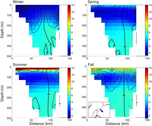
We also compared our simulated transport with unpublished estimates made by Denis Gilbert (Maurice Lamontagne Institute, personal communication, 2013) from current measurements made from May to September 1996, which gave a total outflow of 0.86 Sv and a total inflow of –0.78 Sv. Comparatively, we obtain a total outflow of 0.9 Sv and a total inflow of –0.7 Sv over the same period (average of May to September for 2006 to 2010).

c Temperature and Salinity

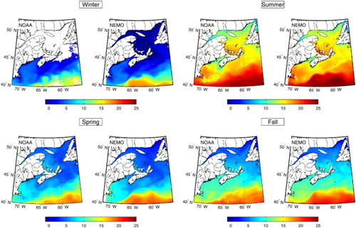
Although some discrepancy is observed with the wind forcing, the simulated surface air temperature used as forcing fits well with observations at different stations around the GSL (Figs 5b, 5d, and 5f). The annual cycle of sea surface temperature (Fig. 7), which correlates with the surface air temperature (Galbraith, Larouche, Chassé, & Petrie, 2012), compares very well with the sea surface temperatures obtained from the Maurice Lamontagne Institute remote sensing laboratory over the entire model domain in 2009.

Fig. 7 Comparison of seasonal sea surface temperatures (in °C) between the satellite and the model (Control run) for 2009. The SST data are generated using NOAA Advanced Very High Resolution Radiometer (AVHRR) satellite images.

The vertical structure (Fig. 6) and composition of the different water masses found in the GSL are also well reproduced by the model year-round. In Fig. 8, we compare all the in situ vertical temperature and salinity profiles acquired by the Department of Fisheries and Oceans in 2009, mainly as part of the Atlantic Zone Monitoring Program, with the corresponding temperature and salinity from the model at the same location and on the same date. The agreement between the observed and simulated values is evaluated with the root mean square error (RMSE; Table 1).

Fig. 8 Observed (conductivity, temperature, depth (CTD) sensor) and simulated (NEMO) monthly T-S diagrams of the water masses in the GSL in 2009 at corresponding locations, shown on map (colours), and times. Simulated water masses have the same composition as observed water masses. Temperature units on the y-axis are °C.

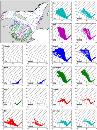
Table 1 RMSEs for salinity and temperature from the Control run in 2009 and the data presented in Fig. 8.

	March	April	May	June	July	August	September	October	November
Salinity	0.58	1.62	0.65	0.69	0.60	0.82	0.73	0.61	0.48
Temperature	0.96	1.14	1.17	1.35	1.83	2.78	2.48	1.19	1.38

d Sea-Ice Concentration

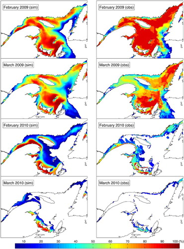
The model also reproduces the seasonal sea-ice cycle reasonably well, as illustrated in Fig. 9, with the comparison of the concentrations obtained from the Control run with the weekly estimates from the Canadian Ice Service. The model reproduces the greater 2009 ice cover, the accumulation over the Magdalen Shallows, as well as ice advection over the Scotian Shelf. The model also reproduces the very light sea-ice conditions observed in 2010. Additional validation of the model performance in reproducing the sea-ice characteristics of the system can be found in Brickman and Drozdowski (2012). Using a model similar to ours, Urrego-Blanco and Sheng (2014a) describe in detail the thermodynamics and dynamics of sea ice in the GSL.

Fig. 9 Sea-ice concentration in February and March of 2009 and 2010, with (left) the Control run and (right) the weekly estimates from the Canadian Ice Service.

In conclusion, taking into account the limitations of such comparisons between model outputs and in situ observations, we consider that our model has the ability to reproduce the seasonal cycle of the horizontal and vertical temperature, salinity, sea ice, and circulation fields of the entire GSL, as well as the complex circulation of the nwGSL and LSLE. It can, therefore, be used to investigate the physical processes leading to krill import in the estuary. Additional capacities of the model applied to fish larval drift in this region can be found in Ouellet et al. (2013).

4 Results

a Two Seasonal Circulation Modes

The model results show two circulation modes. One in the winter–spring period, called Mode 1, and one in the summer–fall period named Mode 2. In Mode 1, the Anticosti Gyre is well defined at all depths (Figs 3a, 3b, 3e, and 3f) and the LSLE surface outflow exits the estuary via a north-shore current that bifurcates south close to Baie-Comeau in winter (Figs 3a and 10a) and near PdM in spring (Figs 3b and 10b) and reinforces the Gaspé Current. Another characteristic of Mode 1 circulation is a reduction in the mean westward currents north of Anticosti Island, accompanied by an intensification of the circulation around the southeastern tip of the island, in both layers (Figs 3a, 3b, 3e, and 3f). At depth, part of the water that circulates around the southeastern tip of the island is entrained by the outflowing water along the southern slope of the Laurentian Channel, but another part of the flow remains close to the island's south shore, making its way upstream to the nwGSL, especially in winter (Fig. 3e). The upstream transport in the deep layer of the LSLE is also intensified (Figs 10e and 10f).

Fig. 10 Enlarged version of Fig. 3. Mean 2006–2010 currents averaged over krill mean nighttime ((a) to (d) 0–40 m) and daytime ((e) to (h) 80–180 m) depths for each season in the LSLE and nwGSL. The location of the PdM transect is displayed in (g), with the northern portion (nPdM) in grey and the southern portion (sPdM) blank. Blue arrows indicate westward-flowing currents and red arrows eastward-flowing currents.

In Mode 2, the circulation in the nwGSL follows a “C” shape (i.e., the gyre is not closed west of Anticosti Island), the circulation along the GSL north shore intensifies (north of Anticosti Island up to PdM; Figs 3c and 3d), and the flow around Anticosti Island is reduced. The upper-layer circulation along the north shore of the LSLE changes direction, from a dominant downstream to an upstream flow, while the outflow from the LSLE is constrained to the south shore (Figs 3c, 3d, 10c, and 10d). In Mode 2, we thus have a somewhat continuous flow along the GSL and LSLE north shores, from SBI to the head of the Laurentian Channel. In the deep layer (80–180 m), the mean upstream flow is reduced compared with Mode 1. This reduction results, in part, from changes in vertical stratification and in part from the advection of the CIL into the LSLE. After restratification of the water column by increased runoff and solar insolation in spring and summer, the CIL is the layer that is principally advected towards the Laurentian Channel head. The deeper Atlantic layer that had been uplifted during winter deepens and flows in the opposite direction (outward), on average. In summer, the inflection point (between inflow and outflow) occurs at depths ranging between 110 and 170 m. Averaging over the 80–180 m layer thus leads to small currents over that period. In the fall, the inflection point gradually deepens. In summer, the inflow peaks at around 50 m, whereas in winter it peaks around 120 m.

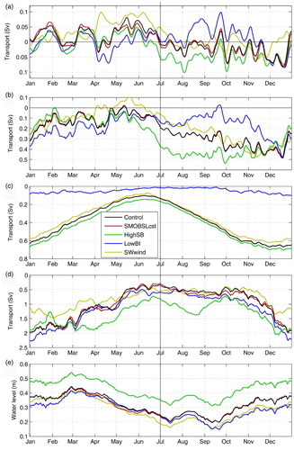
These two circulation modes correspond to transport changes at the bounding straits (SBI and Cabot Strait), at the Jacques-Cartier Strait (JCS) and nPdM transects (nPdm located on Fig. 10g), and in the mean LSLE water level (Fig. 11). A clear shift in the mean transport at nPdM (five-year average), from positive (outflow) to negative (inflow), can be seen in July (Fig. 11a). From January to June (Mode 1), the transport at SBI and eastern Cabot Strait decreases, reaching a minimum in June (Figs 11c and 11d). During that period (Mode 1), the transport at JCS is low and sometimes in the reverse direction (i.e., flow towards the northeast GSL, Fig. 11b). In contrast to Mode 1, the inward transport at SBI and Cabot Strait increases during the July to December period (Mode 2), reaching a maximum in December (Figs 11c and 11d). The westward transport at JCS increases, also reaching a maximum around December (Fig. 11b). During Mode 2, the transport at nPdM becomes negative (inflow to LSLE, Fig. 11a), and the mean water level in the LSLE generally increases (Fig. 11e).

Fig. 11 Yearly time series of the seven-day moving average of (a) 0–40 m averaged transport across the nPdM cross-section, (b) transport across JCS, (c) transport across SBI, (d) transport at the eastern half cross-section of Cabot Strait, and (e) mean water level in the LSLE (between the Saguenay Fjord and PdM), for the five years of the simulation. The bold line on each panel is the five-year mean. The vertical line represents the approximate timing of the mean circulation shift. Negative transport denotes inward transport (i.e., westward).

b Wind-Forced Inflow Events at PdM

In order to determine which processes control the advection of krill from the nwGSL to the LSLE, we examined the transport across the nPdM cross-section for each year (2006 to 2010; see Fig. 12 which displays the results for 2009) as well as the mean circulation in the region. Even though clear seasonal patterns were derived (e.g., Figs 3 and 10), Figs 12b to 12d show that current reversals at the nPdM section are frequent. Surface inflow along the north shore occurs at different times of the year (February, April, July, October, November, and December) over periods of variable duration, from a few days up to about 40 days (e.g., end of June to beginning of August 2009). The inflow events at PdM are also apparent in the 80–180 m layer (Fig. 12c), although they are damped when the CIL is present (June to November), as mentioned in Section 4a.

Fig. 12 (a) North–south (thin line) and east–west (bold line) component of the mean winds over the GSL, north of Îles de la Madeleine (positive pointing north or east). Mean daily transport across the two PdM half sections (see Fig. 10g) in 2009, nPdM (thick line), and sPdM (thin line) and over three different layers: (b) 0–40 m, (c) 80–180 m, and (d) entire water column for the Control run and for the sensitivity analysis with constant runoff over the year for the large rivers flowing into the LSLE (SMOBSLcst, see Section 2d). The large negative pulses at nPdM are indicative of inflow events (grey shading), and the arrows point to the two inflow events detailed in Fig. 13.

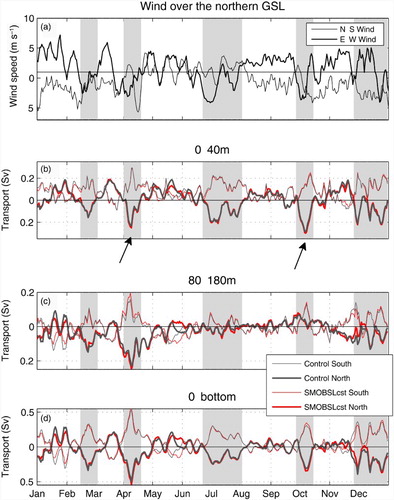
There is a clear correlation between the inflow events at nPdM (Figs 12b to 12d) and the eastern component of the winds over the GSL (Fig. 12a). The maximum correlation between the east–west wind component and the flow in the 0–40 m layer (R = 0.61) is found at a four-day lag. Analyzing daily weather maps produced by NOAA (http://www.wpc.ncep.noaa.gov/dailywxmap/), we found that, in most cases, the inflow events were associated with the passage of extratropical depressions travelling from the west with their centre passing over the southern GSL (which is the zone with a higher frequency of cyclones in the area (Piccolo & El-Sabh, 1993)). Isobars for these systems tend to align with the north shore of the GSL during their northeastward displacements and as the winds rotate cyclonically around the low pressure centre, alongshore winds develop. These alongshore winds, which cause Ekman transport towards the coast, then lead to a sea level set-up along the shore and to an acceleration of the westward alongshore flow in the northwest GSL. This alongshore flow then maintains its path along the coast, as well as around the bend at PdM, and intrudes into the LSLE. Intrusions of GSL water into Chaleur Bay following an intensification of the Gaspé Current were also observed by Gan, Ingram, and Greatbatch (1997).

This coastal set-up effect is shown in (Figs 13a and 13d) and Figs 13c and 13f, which illustrate the inflow events indicated by the arrows on Fig. 12, as well as one case when no inflow occurs (Figs 13b and 13e). We can see the higher sea level along the north shore of the GSL and the inflowing currents at PdM on 7 April and 5 October. These events were also measured by the ADCPs. We can clearly see the southward accelerating currents at M2 in April 2009 on Fig. 4, as well as the inflowing currents at M3 in both layers. The October inflow was also captured by the ADCP at station M3b. Unfortunately, we had no measurements at the M1 and M2 moorings during that time. However, the current reversal simulated at M2 on 2 May 2009 (Fig. 13b) was captured by the ADCPs (Fig. 4, M2, 10–40 m).

Fig. 13 Circulation and wind conditions during the two nPdM inflow events indicated by the arrows in Fig. 12 and a no-inflow case on 2 May. (a), (b), and (c) Daily vertically averaged current for the surface layer (0–40 m) overlain on the surface salinity. The insets show current speed cross-sections across the PdM transect (negative values are upstream). (d), (e), and (f) Daily wind stress calculated by the atmospheric model and used to force the ocean circulation model overlain on the daily mean water level.

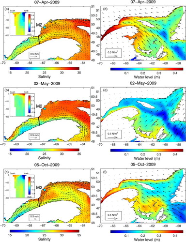
We found that the inflow events occurred over greater depths (down to 250 m) in winter and spring, whereas they were more intense and constrained closer to the surface and the north shore in summer and fall (not shown but see insets in Fig. 13a for spring and Fig. 13c for fall). These differences result from changes in stratification and water mass composition that affect the vertical structure of the circulation. In summer and fall, mostly the surface and CIL layers are advected into the LSLE.

Inflow through the nPdM section is generally mirrored by outflow through the sPdM section (Fig. 12). During the main inflow events, outflow along the south shore lags the inflow along the north shore by three days in the 0–40 m layer (in all five years analyzed) but precedes it by one or two days in the 80–100 m layer (depending on the year). Inflow events also lead to a rise in the mean sea level of the LSLE (e.g., Figs 13d and 13f). These mean sea level rises can also be clearly seen in Fig. 11e for three major events (August 2008 and March and December 2010).

c Krill Distribution and Transport

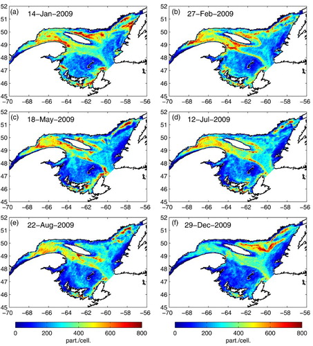
We now examine the effect of the seasonal circulation and inflow events on the transport of migrating krill (MIGR simulation) in the GSL and towards the LSLE in 2009 (Fig. 14). In January (beginning of Mode 1), a little over one month after a uniformly distributed release on 1 December 2008, simulated krill are gradually advected out of the LSLE and aggregations form along the Gaspé Peninsula. Krill found in the northeast GSL are advected north of Anticosti Island where they accumulates (Fig. 14a). Krill that accumulated north of Anticosti Island then moved around the southeastern corner of the island and along the southern shore to reach the nwGSL at the end of February (Fig. 14b). During April and May, krill accumulate in the nwGSL (with krill coming from both south and north of Anticosti Island; Fig. 14c). At the beginning of July (Mode 2), the seasonal circulation regime shift occurred and the krill found in the nwGSL, near PdM, were advected towards the LSLE (Fig. 14d). In August, the inflow of krill into the LSLE diminishes and the number of krill found in the LSLE starts to decline (Fig. 14e). Some recirculation and inflow events (containing smaller numbers of krill) occurred during the fall, and in December the cycle started over with important accumulation of krill north of Anticosti Island (Fig. 14f).

Fig. 14 Daily mean krill density at each grid cell (integrated number of particles from the surface to the bottom) at different times of 2009 for the DVM krill scenario (MIGR). The initial density on 1 December of the previous year was 400 individuals per horizontal cell.

To investigate in more detail the impact of the two circulation modes and of the set-up of the simulations (start up in December and number of initial particles), we looked at the average number of particles in the LSLE obtained for the three krill scenarios (MIGR, DAY, and NIGHT; Fig. 15) for the yearly runs and for the five-year simulation. The first thing we note is that running yearly or five-year simulations does not affect our analysis. The main difference between the two set-ups is that particles found in the surface layer in the LSLE in the yearly run are flushed out over the entire Mode 1 period, except during the inflow events (Figs 15a and 15c). This leads to a decrease in the total number of particles found in the LSLE, even when the particles are migrating and although the inflow of krill at depth is more important, as illustrated with the DAY simulation (Fig. 15b). This important decrease results from the advection of krill out of the LSLE during their night stay at the surface (Fig. 15c). After winter, krill density from the MIGR experiment continues to decrease. This is not unexpected because of the imbalance between the initial conditions (400 particles per cell), the inflow of particles at the eastern boundaries (200 particles per cell), and the lack of production inside the boundaries of the model.

Fig. 15 Mean krill density (number of individuals per vertically integrated grid cell) in the LSLE (between the Saguenay Fjord and PdM) for each year and for the three vertical distribution scenarios (MIGR, DAY, and NIGHT) (a), (b), and (c) for the yearly simulations and (d), (f), and (e) for the five-year simulations, each year being represented separately for comparison with the yearly simulations. The initial density on 1 December of the previous year was 400 individuals per horizontal cell for the yearly simulations. The five-year run started on 1 December 2005. Note that the vertical scale of the DAY simulation is twice as large as for the other simulations. For the five-year DAY scenario (e), in which LSLE krill steadily accumulate, the krill density at the beginning of each year was brought down to 500 for the comparison (actual mean densities at the end of each year were 894, 1020, 1296, 1432, and 1509 individuals per grid cell for 2006 to 2010, respectively).

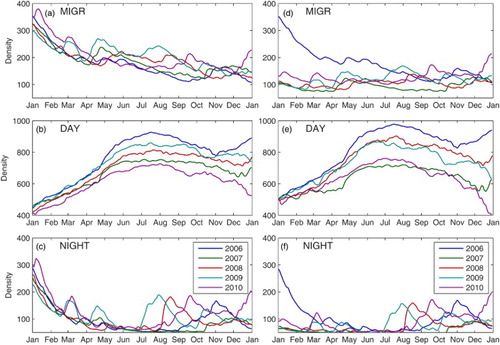
To determine the relative importance of krill transport towards the LSLE when they are at their daytime depths compared with when they are at their nighttime depths, we calculated the monthly mean inflow and outflow across the mouth of the LSLE (full PdM transect) with the MIGR simulation of the five-year run for the years 2007 to 2010 (shown in Fig. 15d). During these four years, the monthly mean krill inflow was always more important in the deep layer (80–180 m) over the entire Mode 1 period. In Mode 2, the mean inflow is also more important in the deeper layer except for those months when inflow events occurred (i.e., October and November 2007; August and November 2008; July, October, and December 2009; and August, September, and December 2010). The simulated increases in the number of particles in the Mode 2 period in (Fig. 15d) all corresponded to these events.

These experiments highlight the importance of krill inflow at depth during the first half of the year and the importance of surface inflow at nPdM during the second half of the year for the maintenance of a krill population in the LSLE. Indeed, Figs 15b and 15e show that the number of particles in the DAY simulations decreases in Mode 2, while it increases by pulses for the krill remaining at the surface at all times (Figs 15c and 15f). These figures also reveal that particles remaining in the surface layer at all times are retained within the GSL system and accumulate in the nwGSL, where they are available for advection into the LSLE during the passage of a storm.

5 Sensitivity analyses

In this section, different sensitivity analyses are performed to test the relative importance of the main forcings on the timing of the circulation shift between Mode 1 and Mode 2 and on the inflow events.

a Constant Runoff in the LSLE

Koutitonsky et al. (1990) attributed the observed circulation shift at the end of July 1979 to the seasonal decrease in runoff in the LSLE. Saucier et al. (2009) found a weak (though significant) negative correlation between freshwater runoff and the 0–30 m surface transport at PdM. They suggested that the runoff variability could have an impact on the inflow of water from the nwGSL at nPdM. To investigate whether freshwater runoff could indeed have an effect on the seasonal circulation shift (from Mode 1 to Mode 2) and on the inflow events at the mouth of the LSLE, we performed a simulation with the runoffs from the main rivers flowing into the St. Lawrence Estuary set to their annual mean (SMOBSLcst, Section 2d).

River runoff has an important impact on the stratification, tidal upwelling, mixing, and entrainment of deeper water at the head of the Laurentian Channel, as well as on the estuarine circulation (e.g., Ohashi & Sheng, 2013; Saucier et al., 2009). However, our results show that suppressing the runoff seasonal variability does not affect the timing of the inflow events at nPdM in general (Figs 12b to 12d). Similarly, it brings only small changes to the circulation features described in Section 3a (Figs 16a and 16b). These results show that seasonal changes in river runoff from the main LSLE rivers do not control the circulation shift at the mouth of the LSLE and in the nwGSL as suggested by Koutitonsky et al. (1990). However, modifying the runoff strength does have an impact on the transport across the nPdM and eastern Cabot Strait cross-sections although the departures from the Control run are small (Figs 17a and 17d).

Fig. 16 Mean currents in the 0–40 m layer for the summer with (a) the Control simulation and the sensitivity analyses, (b) SMOBSLcst, (c) LowBI, (d) HighSB, and (e) SWwind, with the mean 0–40 m summer salinity colour mapped, as well as (f) the climatological (1971–2000) mean 0–40 m salinity.

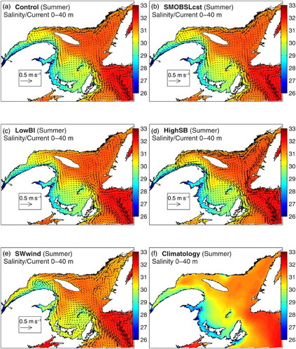
Fig. 17 As in Fig. 11, but showing only the five-year means for the Control simulation and the sensitivity analyses. Seven-day moving average of (a) transport across the nPdM cross-section averaged over the 0–40 m layer, (b) transport at JCS, (c) transport at SBI, (d) transport at the eastern half of Cabot Strait, and (e) mean water level in the LSLE (between the Saguenay Fjord and PdM. The vertical line represents the approximate timing of the mean circulation shift. Negative transport denotes inward transport (westward).

b Modified Transport at SBI and Cabot Strait

From the transport presented in Fig. 11, we concluded that the circulation shift at nPdM (from Mode 1 to Mode 2) was largely caused by the changes in transport (from decelerating to accelerating) at the bounding straits. To further investigate the impact of the transport at SBI and Cabot Strait on the dynamics of the exchanges between the nwGSL and the LSLE, we performed two additional sensitivity analyses (LowBI and HighSB) described in Section 2d. Figure 3 was reproduced with all the sensitivity analyses for comparison of the results and description of the changes (figures not shown).

The transport at SBI obtained with the LowBI simulation is shown in (Fig. 17c). The large reduction in transport at SBI in winter led to a weaker coastal current along the north shore between La Romaine and SBI, to a reduction in the current deflection observed at La Romaine (Fig. 3), and consequently to a stronger coastal current along the north shore west of La Romaine. These changes are reflected in the intensified westward transport at JCS (Fig. 17b) and reduced outflow and increased inflow at nPdM (Fig. 17a).

In spring, the flow coming through SBI is further off the coast, which leads to a stronger circulation around Anticosti Island through Honguedo Strait. The changes in the transport at JCS are small (Fig. 17b) but, combined with the intensified circulation south of Anticosti Island, they intensify the Anticosti Gyre and the inflow at nPdM in April and reduce the outflow in May and June (Fig. 17a). In summer, the circulation along the north shore is considerably reduced (Figs 16a, 16c, and 17b), and there is no inflow at nPdM, except for a short period in early August (Fig. 17a).

In fall, the reduced circulation along the north shore even led to the reversal of the gyre in the nwGSL (from cyclonic to anticyclonic). But most importantly, Fig. 17a shows that there are no longer two circulation modes at nPdM, with inflows occurring mainly in April and in December. The circulation in the deep layer (80–180 m) is, in general, also reduced. Some of these findings were also reported by Smith, Saucier, and Straub (2006a) and Urrego-Blanco and Sheng (2014b) in their simulations with a closed SBI.

The sensitivity analysis to the transport at Cabot Strait was made by increasing the open boundary inflow along the eastern boundary at SB (see Section 2d). Increasing the shelf-break transport led to a larger inflowing transport at eastern Cabot Strait from spring to fall but to a decrease in winter (Fig. 17d). The reduced inflow at eastern Cabot Strait resulted in reduced transport at JCS but not at nPdM (Figs 17a and 17b) because of the intensified upstream circulation south of Anticosti Island (not shown). In spring, the inflow at eastern Cabot Strait is greater but the changes at JCS and nPdM are small, except in June, when westward transports are greater (Figs 17a and 17b), leading to an earlier regime shift by two to three weeks. The greater inward transport at eastern Cabot Strait led to an intensification of the currents along the western Newfoundland coast which in turn strengthened the westward coastal current along the north shore of the GSL, which then slightly intensified the circulation in the Anticosti Gyre in the nwGSL (Figs 16a, 16d, 17a, and 17b). Simulating realistic transport at Cabot Strait thus appears important in obtaining a realistic aggregation of krill in the nwGSL and in the LSLE during the summer–fall period.

c Constant Southwest Wind Direction

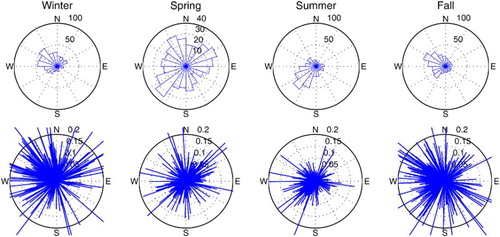
Figure 18 shows the direction from which the wind blows for each season. In winter, strong northwest winds dominated, whereas in summer, weaker southwest winds dominated. In spring, the direction of the wind is more variable, with a larger contribution of eastern winds relative to the other seasons, while in fall, western winds are dominant. In this simulation, we kept the sign of both wind components positive, effectively keeping the winds blowing from the southwest quadrant. In winter, this change in direction led to a large reduction in inflow at eastern Cabot Strait and to a somewhat smaller reduction in fall (Fig. 17d). Using constant atmospheric forcing, Urrego-Blanco and Sheng (2014b) also noticed the strong influence of wind variability on the transport at Cabot Strait.

Fig. 18 Wind roses for each season for the northern GSL, (upper) total number of days with the wind blowing from each direction between 2006 and 2010, (lower) wind stress intensity from the corresponding directions.

The fall and winter transports at SBI were also reduced (Fig. 17c) because of higher sea levels in the northeast GSL. In spring, the outflow at nPdM intensifies (Fig. 17a), and the alongshore current between nPdM and La Romaine flows in the reverse direction (as illustrated by the reversed transport at JCS; Fig. 17b). There is still a circulation regime shift in July, although delayed by a few weeks (Fig. 17a). Although the mean transports at nPdM in Mode 1 are now mainly outflowing, there is an oscillation between outflow and inflow in Mode 2. The sensitivity analyses thus confirm the importance of the transport at the bounding straits and of the variable wind direction on the presence of two circulation regimes (Mode 1 and Mode 2) in the GSL.

6 Discussion

As reported by different authors (e.g., Koutitonsky et al., 1990; Mertz et al., 1989), we noted a seasonal shift in the circulation at the mouth of the LSLE during summer (Fig. 11a). Numerous week-long inflow events from the nwGSL into the LSLE along the north shore are sporadically superimposed on the mean seasonal circulation patterns. These inflow events were attributed to the passage of atmospheric depressions above the GSL and sustained easterly winds, which generate an elevation of the water level along the north shore and an acceleration of the coastal currents towards the LSLE. The coastal current then remains attached to the coast at PdM in a manner similar to the Gaspé Current that remains attached to the coast and intrudes into Chaleur Bay when in an acceleration phase (Gan et al., 1997). The effect of inflowing events on krill transport into the LSLE will depend on the accumulation, or not, of krill near PdM in the previous months or weeks. Some of these processes are discussed in more detail in the following subsections.

a Seasonal Circulation Shift at the Beginning of Summer

Many forcings act simultaneously on the GSL, and it has been difficult to separate the effect of each one (Koutitonsky & Bugden, 1991; Saucier et al., 2009). Koutitonsky et al. (1990) observed a circulation shift at the end of July 1979 that they attributed to the decrease in runoff in the LSLE. Mertz et al. (1988), using the same dataset, noted a reduction in the current variability at the mouth of the LSLE when the shift occurred in July 1979. Smith et al. (2006a, 2006b) also suggested that a seasonal change occurred in the nwGSL circulation which affected the CIL and deep-layer circulation in the LSLE. However, the shift in their observations occurred at the end of March 2003 when multiple intense extratropical storms successively crossed the region (between 25 March and 6 April; http://www.wpc.ncep.noaa.gov/dailywxmap/). The sudden appearance of the CIL in the LSLE observed by Smith et al. (2006a) could thus result from an inflow event, as described in our study. We suggest that the simulated seasonal circulation shifts (early winter and early summer) result from a combination of the two main forcings: (i) large-scale atmospheric forcing (greater than the GSL scale), which influences the circulation along the Labrador and Newfoundland coasts and the transport at SBI and Cabot Strait (Han et al., 2008) and (ii) the variability of atmospheric forcing at the scale of the GSL through direct forcing of coastal currents along the north shore of the GSL and through changes in transport at Cabot Strait.

A strong westward coastal current is generated along the north shore of the eastern GSL (Fig. 3a) by the stronger transport at the SBI in winter (Fig. 11c; Petrie et al., 1988). This coastal current is partially deflected southward in the vicinity of La Romaine (Figs 1 and 3a). This change in the direction of the current is accompanied by a reduction in the westward circulation north of Anticosti Island and by an intensification of the currents around the southeastern tip of Anticosti Island (Figs 3a and 3e). Although many different forcings could explain this deflection (e.g., changes in the lateral salinity gradient, lower stratification that leads to stronger barotropicity and topographic steering, strong and persistent northwesterly winds), our sensitivity analysis showed that reducing the SBI transport in winter led to a coastal current located further offshore and to a reduction in the southward deflection at La Romaine (i.e., the current followed the topography better around the tip of the topographic feature near La Romaine).

In spring, the transport at SBI is reduced, as is the transport at JCS, with the mean even displaying a reversal in direction in May (e.g., towards the northeast GSL). At the end of June, the transport at SBI starts to increase after reaching a minimum (Fig. 11c); the coastal current accelerates and remains attached to the coast near La Romaine, leading to stronger coastal currents from La Romaine to PdM (Fig. 3c). The winter–spring circulation configuration is ready to be tipped over. We showed that the tipping of the circulation is caused by the passage of a storm. Thus, as suggested by Mertz et al. (1992), changes in the basic state of the circulation change the characteristics of the response of the system to wind forcing.

b Accumulation of Krill in the nwGSL

For significant amounts of krill to be advected into the LSLE, large aggregations must first form in the nwGSL and near PdM. The nwGSL is indeed the known source of krill for the LSLE (see review by Simard, 2009). Even though the initial spatial distribution is uniform, krill rapidly (within days) form aggregations along shelf breaks as a result of tidal effects and other high-frequency oscillations. Even though the currents used for particle advection are daily averages, there are still some tidal effects in the circulation because both the diurnal and semi-diurnal constituent periods do not coincide exactly with the length of the day (except for S2 at some locations). Maps et al. (2015), using the same daily average currents, found that convergence zones generated by topographic forcing and sheared horizontal currents explained over 50% of the observed krill aggregations in the GSL. The inclusion of higher-frequency flows certainly has an impact on the aggregation and retention of krill in the LSLE (e.g., Cotté & Simard, 2005; Lavoie et al., 2000). The impact is less known in the GSL, but it would most likely lead to a greater concentration of krill in the patches found along the shelf edges.

Aggregations form north of Anticosti Island in winter and later make their way towards the nwGSL, around the eastern tip and up the southern side of Anticosti Island. Krill are also advected north of Anticosti Island, especially when krill are in the surface layer (see narrow shallow channel (<80 m) in JCS on Fig. 1 inset) and principally in April and May after the reduction in the dominant northwesterly winds (e.g., Fig. 18). Inflow events before that period also result in the passage of krill from north of Anticosti Island towards the nwGSL along the north shore. Sensitivity analysis with the DVM model, which resulted in our shallow (<100 m) daytime vertical distribution (Fig. 2), showed that the formation of aggregations along shelf breaks and over shallow plateaus is important for krill travelling along the north shore of the GSL and around Anticosti Island to make their way to the nwGSL. Indeed, a large amount of krill found south of Anticosti Island in February and March that are not hugging the island shelf break are likely to be caught in the outflowing current and advected out of the GSL towards the Scotian Shelf.

To verify that the uniform initial krill distribution was not influencing our analysis we made an uninterrupted five-year simulation (Fig. 15). Fewer particles remained in the system, but the general features described above were still present. Although few data are available to validate the simulated accumulation of krill in the northeast GSL (e.g., Berkes, 1976) in winter (Fig. 8f), it appears essential for the subsequent accumulation of krill in the nwGSL. In turn, a certain amount of particle inflow at SBI and Cabot Strait is necessary to maintain this feature from one year to the next in the five-year simulation.

c Krill Transport into the LSLE

In general, the simulated quantity of krill present in the LSLE decreases faster in winter and spring. The upstream transport in the 80–180 m layer at this time of year is greater than in summer and fall (Figs 3e to 3h) but so is the flushing at the surface along the north shore (Figs 3a to 3d), which, in the end, leads to a decrease in mean krill density (Fig. 15a). The effect of this circulation mode on krill transport is also obvious in Figs 15b and 15c, with a doubling of krill density in the LSLE for the krill remaining at depth at all times and of a rapid flushing of nearly all krill that reside in the surface layer at all times. During inflow events, both the surface and the deeper layers flow upstream along the north shore of the GSL, leading to an increase in krill density in both the migrating and surface-dwelling (NIGHT) krill (Figs 15a and 15c).

The end of spring is a period of transition when the GSL system changes from a two-layer to a three-layer system with the formation and advection of the CIL. At the head of the Laurentian Channel, the increase in stratification leads to the advection of CIL water, rather than the deep Atlantic layer (e.g., Lavoie et al., 2000; Saucier et al., 2009). Thus, there is a faster upstream advection of CIL waters at nPdM while an outflow of the deep layer sometimes occurs. The averaging of these two layers (inflowing and outflowing) leads to the small average currents observed for the 80–180 m layer in summer (see Figs 3g and 10g). The advection of krill remaining at their daytime depths (DAY) consequently slows and the total number of krill in the LSLE sometimes decreases (Fig. 15b), until the deepening of the surface layer in November and December.

As mentioned earlier, for a circulation inflow event to translate into a significant krill inflow event, a certain quantity of krill must be present in the nwGSL near PdM. Our model focuses on the control of krill transport and only accounts for the main vertical distribution behaviour of adult krill. It ignores the intrinsic population dynamics (growth, mortality, age, and size-dependent behaviours, etc.) and is thus lacking important population increase and decrease factors. However, we can say that favourable conditions for inflow and retention into the LSLE are not met in winter (except in 2010 due to anomalous easterly winds in winter) because of both the circulation and the longer residence time of krill in the upper layer in response to the longer nighttime.

In our simulations, the quantity of krill present in the nwGSL and available for transport within the LSLE in summer and fall depends, in large part, on the wind forcing that prevailed in winter and spring over the GSL. The latter indeed determines the size and locations of krill aggregation prior to the passage of atmospheric depressions. Thus, the large interannual variability of LSLE krill density observed in the MIGR simulation (Fig. 15a) results, in part, from the quantity of krill that accumulated in the nwGSL during spring and, in part, on the strength and duration of the inflow events generated by the passage of atmospheric depressions in the GSL. Once the PdM entrance to the LSLE is crossed, the extent of krill inflow towards the head of the Laurentian Channel and the residence time in the LSLE are subject not only to the large-scale dynamic processes presented above but also to smaller-scale ones, such as the ones discussed by Lavoie et al. (2000). Of course, with the coarse resolution of our present large-scale modelling, the dense krill aggregation observed at the head of the Laurentian Channel (Simard, 2009; Simard & Lavoie, 1999) cannot be replicated.

5 Conclusions

Our study attempted to explain the physical processes controlling the exchanges of krill between the nwGSL and the LSLE. We found that the average circulation switches between two regimes: Mode 1 covering winter and spring and Mode 2 covering the summer and fall. The seasonal circulation regimes are governed by the transport at SBI and Cabot Strait and by wind forcing at the scale of the GSL. The timing of flow reversal near PdM appears to be determined by the passage of extratropical cyclones that, depending on their trajectory, generate a sea level set-up along the north shore of the GSL, leading to strong coastal currents in the direction of the wind component parallel to shore that propagate into the LSLE. Depending on whether the conditions during the previous months were favourable or not for important krill accumulation in the nwGSL, these inflow events can translate into massive entry of krill into the LSLE, where important whale feeding areas are found.

The importance of krill inflow to the surface layer along the north shore of the LSLE for the maintenance of the large aggregations found at the head of the Laurentian Channel was not fully appreciated before this study (but see companion paper by Maps et al., 2013). The surface layer was traditionally considered mainly as an exit conduit (Simard, 2009; Sourisseau et al., 2006, 2008). Sourisseau et al. (2006) did not have an accumulation in the estuary when their krill densities were migrating because their circulation model rarely reproduced the surface inflow along the north shore due to their large horizontal mixing coefficients in the LSLE. Our study shows that inflows both at the surface and below are essential for large krill import up to the head of the Laurentian Channel.

This study did not consider local krill production, which will undoubtedly be affected (for better or worse depending on the species) by our changing climate. Moreover, although local production is not accounted for, our study suggests that large quantities of krill are flushed out of the GSL system on a seasonal basis and that inflow of individuals from upstream regions (e.g., Labrador Sea) might be necessary for the maintenance of the populations in the long term.

The projected increase in the GSL freshwater runoff (Lambert et al., 2013) could reduce the overall transport of the deeper layers towards the Laurentian Channel head in the future because of reduced ventilation of the deep layer at the Laurentian Channel head in winter (Saucier et al., 2009). Moreover, changes in transport along the Labrador and Newfoundland shelves, as well as changes in the path, frequency, and strength of storms in the northwest Atlantic region (e.g., Perrie, Yao, & Zhang, 2010; Teng, Washington, & Meehl, 2008; Woollings, Gregory, Pinto, Reyers, & Brayshaw, 2012), will affect the transport of krill towards the GSL and between the different regions of the GSL in the future. Exactly how the transport of the dominant krill species in the GSL (T. raschi and M. norvegica) will be affected remains to be seen because krill abundance and transport in the different regions of the northwest Atlantic will most likely be modified as well.

Acknowledgements

We are grateful to two anonymous reviewers whose comments greatly improved the manuscript, to Dr. Denis Gilbert for providing his transport estimations at Cabot Strait, to Dr. Pierre Larouche for the satellite sea surface temperature data, and to Amin Mohammadpour for the wind and air temperature data.

Disclosure statement

No potential conflict of interest was reported by the authors.

Additional information

Funding

This research was funded by Fisheries and Oceans Canada as part of the Ecosystem Research Initiative in the Lower St. Lawrence Estuary.

References

- Berkes, F. (1976). Ecology of euphausiids in the Gulf of St. Lawrence. Journal of the Fisheries Research Board of Canada, 33(9), 1894–1905. doi: 10.1139/f76-242
- Bobanovic, J., & Thompson, K. R. (2001). The influence of local and remote winds on the synoptic sea level variability in the Gulf of Saint Lawrence. Continental Shelf Research, 21(2), 129–144. doi: 10.1016/S0278-4343(00)00079-0
- Bourgault, D., & Koutitonsky, V. G. (1999). Real-time monitoring of the freshwater discharge at the head of the St. Lawrence Estuary. Atmosphere-Ocean, 37(2), 203–220. doi: 10.1080/07055900.1999.9649626
- Brickman, D., & Drozdowski, A. (2012). Development and validation of a regional shelf model for maritime Canada based on the NEMO-OPA circulation model. Canadian Technical Report of Hydrography and Ocean Sciences, No. 278. Dartmouth, Nova Scotia: DFO.
- Butcher, J. C. (2003). Numerical methods for ordinary differential equations. New-York: John Wiley & Sons.
- Campin, J. M., Adcroft, A., Hill, C., & Marshall, J. (2004). Conservation of properties in a free-surface model. Ocean Modelling, 6(3–4), 221–244. doi:10.1016/S1463-5003(03)00009-X
- Chassé, J., & Miller, R. J. (2010). Lobster larval transport in the southern Gulf of St. Lawrence. Fisheries Oceanography, 19(5), 319–338. doi:10.1111/j.1365-2419.2010.00548.x
- Chiles, J.-P., & Delfiner, P. (2012). Geostatistics: Modeling spatial uncertainty (2nd ed.). New York: Wiley.
- Cotté, C., & Simard, Y. (2005). Formation of dense krill patches under tidal forcing at whale feeding hot spots in the St. Lawrence Estuary. Marine Ecology Progress Series, 288, 199–210. doi: 10.3354/meps288199
- Deines, K. L. (1999). Backscatter estimation using broadband acoustic Doppler current profilers. In Proceedings of the IEEE Sixth Working Conference on Current Measurement, 11–13 March 1997, San Diego, Calif. pp. 249–253. doi:10.1109/CCM.1999.755249
- Drinkwater, K. F., & Pettipas, R. G. (1993). Climatic data for the Northwest Atlantic: Surface wind stresses off eastern Canada, 1946–1991. Data and Reports Hydrography Ocean Science, No. 123.
- Gagné, J. A., Ouellet, P., Savenkoff, C., Galbraith, P. S., Bui, A. O. V., & Bourassa, M.-N. (2013). Rapport intégré de l'initiative de recherche écosystémique (IRÉ) de la région du Québec pour le projet : les espèces fourragères responsables de la présence des rorquals dans l'estuaire maritime du Saint-Laurent. : Secrétariat Canadien de Consultation Scientifique du MPO. Document de recherche 2013/086. Ottawa.
- Galbraith, P. S. (2006). Winter water masses in the Gulf of St. Lawrence. Journal of Geophysical Research, 111, C06022, 1–23. doi:10.1029/2005JC003159
- Galbraith, P. S., Larouche, P., Chassé, J., & Petrie, B. (2012). Sea-surface temperature in relation to air temperature in the Gulf of St. Lawrence: Interdecadal variability and long term trends. Deep-Sea Research II, 77–80, 10–20. doi:10.1016/j.dsr2.2012.04.001
- Gan, J., Ingram, R. G., & Greatbatch, R. J. (1997). On the unsteady separation/intrusion of the Gaspé Current and variability in Baie des Chaleurs: Modeling studies. Journal of Geophysical Research, 102(C7), 15567–15581. doi: 10.1029/97JC00589
- Gilbert, D., & Pettigrew, B. (1997). Interannual variability (1948–1994) of the CIL core temperature in the Gulf of St. Lawrence. Canadian Journal of Fisheries and Aquatic Sciences, 54(Suppl. 1), 57–67.
- Goosse, H., & Fichefet, T. (1999). Importance of ice-ocean interactions for the global ocean circulation: A model study. Journal of Geophysical Research, 104(C10), 23337–23355. doi:10.1029/1999jc900215
- Han, G., Loder, J. W., & Smith, P. C. (1999). Seasonal-mean hydrography and circulation in the Gulf of St. Lawrence and on the eastern Scotian and southern Newfoundland shelves. Journal of Physical Oceanography, 29(6), 1279–1301. doi: 10.1175/1520-0485(1999)029<1279:SMHACI>2.0.CO;2
- Han, G., Lu, Z., Wang, Z. B., James, H. L., Chen, N., & de Young, B. (2008). Seasonal variability of the Labrador Current and Shelf circulation off Newfoundland. Journal of Geophysical Research, 113, C10013, 1–23. doi:10.1029/2007jc004376
- Harvey, M., Galbraith, P. S., & Descroix, A. (2009). Vertical distribution and diel migration of macrozooplankton in the St. Lawrence marine system (Canada) in relation with the cold intermediate layer thermal properties. Progress in Oceanography, 80(1–2), 1–21. doi: 10.1016/j.pocean.2008.09.001
- Koutitonsky, V. G., & Bugden, G. L. (1991). The physical oceanography of the Gulf of St. Lawrence: A review with emphasis on the synoptic variability of the motion. In J. C. Therriault (Ed.), The Gulf of St. Lawrence: Small ocean or big estuary, Canadian special publication of fisheries and aquatic sciences (Vol. 113, pp. 57–60). Ottawa, Ontario: DFO.
- Koutitonsky, V. G., Wilson, R. E., & El-Sabh, M. I. (1990). On the seasonal response of the lower St. Lawrence Estuary to buoyancy forcing by regulated river runoff. Estuarine, Coastal and Shelf Science, 31(4), 359–379. doi: 10.1016/0272-7714(90)90032-M
- Lambert, N., Chassé, J., Perrie, W., Long, Z., Guo, L., & Morrison, J. (2013). Projection of future river runoffs in eastern Atlantic Canada from global and regional climate models. Canadian Technical Report of Hydrography and Ocean Sciences, No. 288, Mont-Joli, Quebec: DFO.
- Lavoie, D., Simard, Y., & Saucier, F. J. (2000). Aggregation and dispersion of krill at channel heads and shelf edges: The dynamics in the Saguenay-St. Lawrence Marine Park. Canadian Journal of Fisheries and Aquatic Sciences, 57(9), 1853–1869. doi: 10.1139/f00-138
- Madec, G. (2012). NEMO ocean engine Note du Pole de modélisation de l'Institut Pierre-Simon Laplace (No. 27): France: Institut Pierre-Simon Laplace, Paris.
- Madec, G., Delecluse, P., Imbard, M., & Lévy, C. (1998). OPA 8.1 ocean general circulation model reference manual. (No. 11). Institut Pierre-Simon Laplace (IPSL), France.
- Maps, F., Plourde, S., Lavoie, D., McQuinn, I., & Chassé, J. (2013). Modelling the influence of daytime distribution on the transport of two sympatric krill species (Thysanoessa raschii and Meganyctiphanes norvegica) in the Gulf of St Lawrence, eastern Canada. ICES Journal of Marine Science, 71, 71, 282–292. doi:10.1093/icesjms/fst021
- Maps, F., Plourde, S., McQuinn, I., St-Onge-Drouin, S., Lavoie, D., Chassé, J., & Lesage, V. (2015). Linking acoustics and Finite-Time Lyapunov Exponents (FTLE) reveals areas and mechanisms of krill aggregation wihtin the Gulf of St. Lawrence, eastern Canada. Limnology and Oceanography. doi:10.1002/lno.10145
- Mertz, G., El-Sabh, M. I., & Koutitonsky, V. G. (1988). Wind-driven motions at the mouth of the lower St. Lawrence Estuary. Atmosphere-Ocean, 26(4), 509–523. doi: 10.1080/07055900.1988.9649315
- Mertz, G., El-Sabh, M. I., & Koutitonsky, V. G. (1989). Low frequency variability in the lower St. Lawrence Estuary. Journal of Marine Research, 47(2), 285–302. doi: 10.1357/002224089785076280
- Mertz, G., Koutitonsky, V. G., Gratton, Y., & El-Sabh, M. I. (1992). Wind-induced eddy motion in the lower St. Lawrence Estuary. Estuarine, Coastal and Shelf Science, 34(6), 543–556. doi: 10.1016/S0272-7714(05)80061-7
- Ohashi, K., & Sheng, J. Y. (2013). Influence of St. Lawrence River discharge on the circulation and hydrography in Canadian Atlantic waters. Continental Shelf Research, 58, 32–49. doi:10.1016/j.csr.2013.03.005
- Ouellet, P., Bui, A. O. V., Lavoie, D., Chassé, J., Lambert, N., Ménard, N., Sirois, P. (2013). Seasonal distribution, abundance, and growth of larval capelin (Mallotus villosus) and the role of the lower estuary (Gulf of St. Lawrence, Canada) as a nursery area. Canadian Journal of Fisheries and Aquatic Sciences, 70(10), 1508–1530. doi:10.1139/cjfas-2013–0227
- Pellerin, G., Lefaivre, L., Houtekamer, P., & Girard, C. (2003). Increasing the horizontal resolution of ensemble forecasts at CMC. Nonlinear Processes in Geophysics, 10, 463–468. doi: 10.5194/npg-10-463-2003
- Perrie, W., Yao, Y. H., & Zhang, W. Q. (2010). On the impacts of climate change and the upper ocean on midlatitude northwest Atlantic landfalling cyclones. Journal of Geophysical Research-Atmospheres, 115, D23110, 1–14, doi:10.1029/2009jd013535
- Petrie, B., Toulany, B., & Garrett, C. (1988). The transport of water, heat and salt through the Strait of Belle Isle. Atmosphere-Ocean, 26(2), 234–251. doi: 10.1080/07055900.1988.9649301
- Piccolo, M. C., & El-Sabh, M. I. (1993). Cyclone climatology of southeastern Canada. Climatological Bulletin, 27(3), 81–95.
- Plourde, S., McQuinn, I. H., Maps, F., St-Pierre, J.-F., Lavoie, D., & Joly, P. (2013). Daytime depth and thermal habitat of two sympatric krill species in response to surface salinity variability in the Gulf of St Lawrence, eastern Canada. ICES Journal of Marine Science, 71, 272–281. doi:10.1093/icesjms/fst023
- Sameoto, D. D., & Herman, A. W. (1992). Effect of the outflow from the Gulf of St. Lawrence on Nova Scotia shelf zooplankton. Canadian Journal of Fisheries and Aquatic Sciences, 49(5), 857–869. doi: 10.1139/f92-096
- Saucier, F. J., Roy, F., Gilbert, D., Pellerin, P., & Ritchie, H. (2003). Modeling the formation and circulation processes of water masses and sea ice in the Gulf of St. Lawrence, Canada. Journal of Geophysical Research, 108(C8), 3269. 1–20, doi:10.1029/2000jc000686
- Saucier, F. J., Roy, F., Senneville, S., Smith, G., Lefaivre, D., Zakardjian, B., & Dumais, J.-F. (2009). Modélisation de la circulation dans l'estuaire et le golfe du Saint-Laurent en réponse aux variations du débit d'eau douce et des vents. Revue des Sciences de l'Eau, 22(2), 159–176. doi: 10.7202/037480ar
- Sheng, J. (2001). Dynamics of a buoyancy-driven coastal jet: The Gaspé Current. Journal of Physical Oceanography, 31(11), 3146–3162. doi: 10.1175/1520-0485(2001)031<3146:DOABDC>2.0.CO;2
- Simard, Y. (2009). Le Parc Marin Saguenay–Saint-Laurent: processus océanographiques à la base de ce site d'alimentation unique des baleines du Nord-Ouest Atlantique. The Saguenay–St. Lawrence Marine Park: oceanographic process at the basis of this unique forage site of northwest Atlantic whales. Rev. Sc. Eau / J. Water Sci., 22(2), 177–197.
- Simard, Y., de Ladurantaye, R., & Therriault, J. C. (1986). Aggregation of euphausiids along a coastal shelf in an upwelling environment. Marine Ecology Progress Series, 32, 203–215. doi: 10.3354/meps032203
- Simard, Y., & Harvey, M. (2010). Predation on northern krill (Meganyctiphanes Norvegica Sars). In A. T. Geraint (Ed.), Advances in marine biology (Vol. 57, pp. 277–306). London, UK: Academic Press.
- Simard, Y., & Lavoie, D. (1999). The rich krill aggregation of the Saguenay–St. Lawrence Marine Park: Hydroacoustic and geostatistical biomass estimates, structure, variability, and significance for whales. Canadian Journal of Fisheries and Aquatic Sciences, 56(7), 1182–1197. doi: 10.1139/f99-063
- Smith, G. C., Saucier, F. J., & Straub, D. (2006a). Formation and circulation of the cold intermediate layer in the Gulf of Saint Lawrence. Journal of Geophysical Research, 111, C06011. 1–18, doi:10.1029/2005jc003017
- Smith, G. C., Saucier, F. J., & Straub, D. (2006b). Response of the lower St. Lawrence estuary to external forcing in winter. Journal of Physical Oceanography, 36(8), 1485–1501. doi:10.1175/JPO2927.1
- Sourisseau, M., Simard, Y., & Saucier, F. J. (2006). Krill aggregation in the St. Lawrence system, and supply of krill to the whale feeding grounds in the estuary from the gulf. Marine Ecology Progress Series, 314, 257–270. doi: 10.3354/meps314257
- Sourisseau, M., Simard, Y., & Saucier, F. J. (2008). Krill diel vertical migration fine dynamics, nocturnal overturns, and their roles for aggregation in stratified flows. Canadian Journal of Fisheries and Aquatic Sciences, 65(4), 574–587. doi: 10.1139/f07-179
- Tee, K.-T. (1989). Subtidal salinity and velocity variations in the St. Lawrence Estuary. Journal of Geophysical Research, 94(C6), 8075–8090. doi: 10.1029/JC094iC06p08075
- Teng, H., Washington, W., & Meehl, G. (2008). Interannual variations and future change of wintertime extratropical cyclone activity over North America in CCSM3. Climate Dynamics, 30(7), 673–686. doi:10.1007/s00382-007-0314-1
- Urrego-Blanco, J., & Sheng, J. Y. (2014a). Formation and distribution of sea ice in the Gulf of St. Lawrence: A process-oriented study using a coupled ocean-ice model. Journal of Geophysical Research: Oceans, 119, 7099–7122. doi:10.1002/2014JC010185
- Urrego-Blanco, J., & Sheng, J. Y. (2014b). Study on subtidal circulation and variability in the Gulf of St. Lawrence, Scotian Shelf, and Gulf of Maine using a nested-grid shelf circulation model. Ocean Dynamics, 64(3), 385–412. doi:10.1007/s10236-013-0688-z
- Woollings, T., Gregory, J. M., Pinto, J. G., Reyers, M., & Brayshaw, D. J. (2012). Response of the North Atlantic storm track to climate change shaped by ocean-atmosphere coupling. Nature Geoscience, 5(5), 313–317. doi: 10.1038/ngeo1438