Climate Comparisons and Change Projections for the Northwest Atlantic from Six CMIP5 Models

Abstract

Key physical variables for the Northwest Atlantic (NWA) are examined in the “historical” and two future Representative Concentration Pathway (RCP) simulations of six Earth System Models (ESMs) available through Phase 5 of the Climate Model Intercomparison Project (CMIP5). The variables are air temperature, sea-ice concentration, surface and subsurface ocean temperature and salinity, and ocean mixed-layer depth. Comparison of the historical simulations with observations indicates that the models provide a good qualitative and approximate quantitative representation of many of the large-scale climatological features in the NWA (e.g., annual cycles and spatial patterns). However, the models represent the detailed structure of some important NWA ocean and ice features poorly, such that caution is needed in the use of their projected future changes. Monthly “climate change” fields between the bidecades 1986–2005 and 2046–2065 are described, using ensemble statistics of the changes across the six ESMs. The results point to warmer air temperatures everywhere, warmer surface ocean temperatures in most areas, reduced sea-ice extent and, in most areas, reduced surface salinities and mixed-layer depths. However, the magnitudes of the inter-model differences in the projected changes are comparable to those of the ensemble-mean changes in many cases, such that robust quantitative projections are generally not possible for the NWA.

Résumé

[Traduit par la redaction] Nous examinons des variables physiques d'importance pour l'Atlantique Nord-Ouest, dans le cadre d'une simulation du passé et de deux simulations du futur, effectuées suivant les profils représentatifs d’évolution des concentrations (RCP), à l'aide de six modèles du système terrestre (ESM), exploités dans le cadre de la phase 5 du projet d'intercomparaison de modèles couplés (CMIP5). Les variables visées sont la température de l'air, la concentration de la glace de mer, la température et la salinité en surface et subsurface de la mer, et la profondeur de la couche de mélange marine. La comparaison des simulations du passé avec les observations indique que les modèles fournissent une bonne représentation qualitative et une représentation quantitative approximative de plusieurs des caractéristiques climatologiques de grande échelle dans l'Atlantique Nord-Ouest (p. ex. des cycles annuels et des configurations spatiales). Toutefois, les modèles représentent mal la structure fine de certaines caractéristiques marines et glaciaires importantes du nord-ouest de l'Atlantique. Ainsi, la prudence s'impose si l'on utilise l’évolution prévue de celles-ci. Nous décrivons des champs mensuels d’« évolution climatique » entre les périodes de vingt ans allant de 1986 à 2005 et de 2046 à 2065, et ce, à l'aide de statistiques d'ensemble représentant les changements que prévoient les six modèles du système terrestre. Les résultats laissent présager une augmentation généralisée des températures, une hausse des températures de la surface de l'océan dans la plupart des régions, une diminution de l’étendue de la glace marine et, dans la plupart des régions, une réduction de la salinité de surface ainsi que de la profondeur de la couche de mélange. Néanmoins, dans plusieurs cas, les écarts entre les modèles qui prévoient ces changements s'avèrent comparables à ceux des moyennes d'ensemble des changements, de façon que des projections quantitatives fiables ne soient généralement pas possibles pour le nord-ouest de l'Atlantique.

KEYWORDS:

• climate change projections
• Northwest Atlantic
• Earth System Models
• air temperature
• ocean temperature
• salinity
• sea ice
• mixed-layer depth

1 Introduction

Projections of future climate change are needed for many applications, including assessments of potential impacts and planning for mitigation and adaptation activities. However, necessary steps for a scientifically sound approach include observational validation of climate models used in developing the projections and understanding the limitations of these models so that uncertainties can be properly represented. Specific challenges include the representation of decadal-scale (taken here as decadal to multi-decadal) variability on global and smaller scales (e.g., Maher, Sen Gupta, & England, 2014), including regional modes of natural variability such as the Arctic Oscillation, the North Atlantic Oscillation (NAO), and the Atlantic multi-decadal oscillation (AMO) (e.g., Chen & Tung, 2014). For example, it is well documented that there is strong natural decadal-scale variability in the Northwest Atlantic (NWA) apparently associated with coupled atmosphere–ice–ocean interactions (e.g., Hurrell & Deser, 2010; Polyakov, Alexeev, Bhatt, Polyakov, & Zhang, 2010; Terray, 2012) and that, at mid-latitudes, the NWA is a complex confluence and transition zone between the western boundary currents of the North Atlantic's subpolar and subtropical ocean gyres (e.g., Dewar, 2001; Loder, Petrie, & Gawarkiewicz, 1998; Zhai, Johnson, & Marshall, 2014; Zhang & Vallis, 2007). This results in the NWA being one of the Earth's more challenging regions for reliable climate change projections (e.g., Knutti & Sedláček, 2013).

The Fourth (AR4; IPCC, 2007) and Fifth (AR5; IPCC, 2013) Assessment Reports of the Intergovernmental Panel on Climate Change (IPCC), together with their referenced studies and climate model simulations available through Phases 3 (CMIP3) and 5 (CMIP5) of the Climate Model Intercomparison Project (e.g., Knutti, Masson, & Gettelman, 2013; Taylor, Stouffer, & Meehl, 2012), provide a broad foundation for climate change projections, particularly on large scales. These reports provide overwhelming evidence for anthropogenic climate change in many variables during the past century on global and hemispheric scales, as well as ensemble projections for future changes on these scales over the next century (albeit with uncertainties). However, they also point to strong spatial and decadal-scale variability in many areas which is much more difficult to predict. For example, a large region of reduced warming in the surface air and ocean in the subpolar North Atlantic has been observed and projected (e.g., see Fig. TS-2 and Box TS.6 in Giorgetta et al., 2013), sometimes referred to as a “warming hole” (Drijfhout, van Oldenborgh, & Cimatoribus, 2012). It has been attributed, at least in part, to an influence of the Atlantic Meridional Overturning Circulation (AMOC) which contributes to the global ocean's regulation of the Earth's climate system. Sea surface temperature (SST) observations (e.g., Loder & Wang, 2015; Polyakov et al., 2010; Ting, Kushnir, & Li, 2014) indicate that the region has been dominated by decadal-scale variability over the past century. There is evidence for linkages among the NAO, AMO, AMOC, and the North Atlantic's major gyres, which have significant implications for future climate change and variability in the NWA. But, these linkages are complex and remain to be unravelled and represented adequately in climate models.

The purpose of this paper is to summarize the results of an exploratory examination of CMIP5 simulations and projections for key variables in or affecting the NWA that was carried out as part of Fisheries and Oceans Canada's (DFO's) Aquatic Climate Change Adaptation Services Program (ACCASP). The examination provided input to a summary of observed trends and projected changes of ocean climate affecting the NWA off Canada for consideration in a DFO climate change impacts assessment (DFO, 2013). More detailed results from the examination, which took an ensemble approach involving six Earth System Models (ESMs), can be found in Loder and van der Baaren (2013). The underlying goals here are to provide indications of the level of agreement between the “historical” simulations from the ESMs and observations and of the ensemble mean and spread of the projected future changes over a period of 60 years. This paper is not intended to be a definitive investigation of past and future climate change in the NWA nor of the particular ESMs examined or the larger CMIP5 ensemble of global Atmosphere–Ocean General Circulation Models (AOGCMs) but rather an initial NWA examination of a subset of models that were available at the time of the DFO assessment.

Although detailed evaluations of the CMIP5 models have been underway for some time (Flato et al., 2013) and many papers have appeared in the literature (e.g., Andrews, Gregory, Webb, & Taylor, 2012; Cheng, Chiang, & Zhang, 2013; Diffenbaugh & Giorgi, 2012; Jones, Stott, & Christidis, 2013; Knutti & Sedláček, 2013; Markovic, de Elía, Frigon, & Matthews, 2013; Sillmann, Kharin, Zhang, Zwiers, & Bronaugh, 2013a, 2013b; Stroeve et al., 2012; Wang & Overland, 2012), reports with rigorous evaluations of these models on ocean basin scales (other than for sea ice in the Arctic) are generally not available. A pragmatic approach was adopted in this work, involving the use of fields that are readily available from a subset of similar models from leading climate modelling institutions.

The ESMs were chosen because of the availability of their output fields at the time the study was initiated from DFO colleagues who were also examining the fields (Christian & Foreman, 2013; Lavoie, Lambert, ben Mustafa, & van der Baaren, 2013a, Lavoie, Lambert, & van der Baaren, 2013b; Steiner, Christian, Six, Yamamoto, & Yamamoto-Kawai, 2014). These models are not necessarily more advanced than other recently available ESMs or other CMIP5 (or CMIP3) AOGCMs in their representation of the regional atmosphere–ice–ocean coupling of physical variables (e.g., heat, freshwater, and momentum), particularly in complex regions such as the eastern Arctic and NWA. In some cases, these ESMs have lower spatial resolution than other AOGCMs (including ESMs) run by their institutions. Thus, the models should be considered a subset of the approximately 50 AOGCMs (including ESMs) examined in AR5 (Flato et al., 2013) and perhaps a representative subset of the ESMs (Steiner et al., 2014), but not necessarily the “best” AOGCMs for representing the NWA.

Considering that Loder and van der Baaren (2013) confirmed the expected finding (e.g., Taylor et al., 2012) that these coarse-resolution ESMs do not resolve the detailed structure of important ice and ocean features in the NWA, one could ask why there is a need for the information in this paper. Our answer is multi-fold: we consider it important that the representation of these features be described and the level of agreement between the models and observations be presented in the literature, in order to help understand the processes in and the limitations of the models, motivate improvements, help determine whether the simulations are adequate for regional downscaling, and alert the community that caution should be used in downscaled projections. The paper also provides the ensemble mean and inter-model variability of the projected 60-year changes in key variables in the NWA, which may be useful in some applications or may provide an indication of potential (or probable) changes and uncertainties.

The paper is organized by variable. After a brief description of the methodology in Section 2, results are presented for surface air temperature (SAT) in Section 3 and sea-ice concentration (SIC) in Section 4. Results are then presented for ocean temperature and salinity in Section 5 and for ocean mixed-layer depth in Section 6. The paper concludes with a discussion of some particular aspects of air–sea coupling in the models’ projections for the NWA in Section 7 and a summary and discussion in Section 8.

2 Models, data, and methodology

a Models and Simulations

The six ESMs whose historical simulations (e.g., Flato et al., 2013; Taylor et al., 2012) were used in the study are listed in Table 1, together with their originating institutions and grid sizes. The atmospheric grid resolution is in the 150–300 km range and the ocean grid resolution typically in the 50–150 km range, which are coarse relative to the scales of the actual coastal geometry, ocean shelf bathymetry, and some ocean circulation features in the NWA and eastern Arctic.

Table 1. Information on the six ESMs examined in the study. Grid sizes are presented as latitude x longitude. Further information can be obtained from the CMIP5 website (http://cmip-pcmdi.llnl.gov/cmip5/), the websites of the institutions which provided the model fields, or the references indicated.

Model Name	Institution	Reference	Atmospheric Grid	Oceanic Grid
CanESM2: Canadian Earth System Model, version 2	EC's Canadian Centre for Climate Modelling and Analysis (CCCma)	Arora et al. (2011)	∼2.8°	∼0.9° × 1.4°
GFDL-ESM2M: Geophysical Fluid Dynamics Laboratory's Earth System Model, version 2M	GFDL of the National Oceanic and Atmospheric Administration (NOAA, USA)	Dunne et al. (2012)	∼2° × 2.5°	0.3°–1°
HadGEM2-ES: Hadley Centre Global Environmental Model, version 2	Met Office Hadley Centre (United Kingdom)	Collins et al. (2011)	∼1.2° × 1.9°	0.3°–1°
IPSL-CM5A-LR: Low Resolution version of the Earth System Model based on the IPSL's Climate Model, version 5A	Institut Pierre-Simon Laplace (France)	Dufresne et al. (2013)	∼1.9° × 3.8°	0.5°–2°
MIROC-ESM: Earth System Model based on the global climate Model for Interdisciplinary Research on Climate	Japan Agency for Marine-Earth Science and Technology, Atmosphere and Ocean Research Institute (The University of Tokyo), and National Institute for Environmental Studies	Watanabe et al. (2011)	∼2.8°	0.5°–1.7° × 1.4°
MPI-ESM-LR: Low Resolution version of the Max-Planck-Institute Earth System Model	Max Planck Institute for Meteorology (Germany)	Giorgetta et al. (2013)	∼1.9°	∼1.6°

The historical simulations from approximately 1850 to 2005 and the forced simulations for Representative Concentration Pathways (RCPs) 4.5 and 8.5 from 2006 to 2100 (Moss et al., 2010; Taylor et al., 2012; van Vuuren et al., 2011) were considered. These RCPs were chosen to approximate the range of potential future atmospheric greenhouse gas (GHG) concentrations, based on recent emissions and discussions about future emissions (Peters et al., 2013). For the 60-year time scale (∼1990s to 2050s) of primary focus here, the future radiative forcing associated with these RCPs is roughly in the range of that of scenarios B1 and A1FI, respectively, from the Special Report on Emissions Scenarios (SRES; Nakićenović et al., 2000) used in AR4 (Knutti & Sedláček, 2013; Rogelj, Meinshausen, & Knutti, 2012). Results are presented here for RCP8.5 which is a “high-emissions” pathway consistent with recent GHG emissions (Peters et al., 2013) and whose mean effective radiative forcing estimated from the CMIP5 ensemble increases from approximately 1.8 W m⁻² in 2005 to approximately 5.4 W m⁻² in 2065 and approximately 7.6 W m⁻² in 2100 (Collins et al., 2013). The projected 60-year changes for RCP4.5, whose mean effective CMIP5 radiative forcing is approximately 3.5 W m⁻² in 2065, are generally a substantial fraction (e.g., ∼70% for SAT) of those for RCP8.5 (Loder & van der Baaren, 2013).

The primary fields examined here are time-averaged (monthly and then bidecadally) horizontal fields from Run or “member” 1 (r1i1p1) of the six ESMs in Table 1, interpolated (using inverse-distance weighting of the four nearest neighbours) onto a common 2° × 2° grid (J. Christian, personal communication, 2012). The key benefit of using these “interpolated bidecadal monthly” fields is that further computations were greatly facilitated by the common grid (instead of dealing with each model's native grid). The disadvantages include some spatial smoothing of the fields and some loss of resolution of the ice and ocean fields in the vicinity of land–ocean boundaries.

The bidecadal monthly means from six successive periods from 1966–1985 to 2066–2085 were examined, with results presented here for the 1986–2005 and 2046–2065 periods. The variables considered (with their acronyms and CMIP5 variable names in parentheses) are surface air temperature (SAT, tas), sea-ice concentration (SIC, sic), sea surface temperature (SST, tos), sea surface salinity (SSS, sos), and the monthly maximum ocean mixed-layer depth (OML-max, omlmax) (see Taylor (2012) for more detail on these variables); SAT is included because it is one of the primary Earth System variables that is changing with increasing GHGs, and it has a strong influence on the upper ocean; SIC is included because it is also changing with increasing GHGs and is a key factor in fluxes between the atmosphere and ocean in the NWA. The ensemble mean for each variable, month, and grid point was computed by arithmetic averaging over the bidecadal means from the individual models, and the inter-model standard deviation (SD_m, for the models about the ensemble mean) and spread (maximum minus minimum value) were used to indicate variability within the ensemble. With six models, the SD_m is approximately twice the standard error (SE) of the mean (2SE = 2SD_m/(6)^1/2 = 0.8SD_m), which can be used in assessing whether the differences between the means in different periods are statistically significant at the 95% confidence level. These interpolated bidecadal monthly fields were further bilinearly interpolated to prescribed positions (e.g., observation sites) to obtain the annual cycles of selected variables at positions of interest.

In addition to the bidecadal means for the above surface variables, the vertical and cross-basin distribution of subsurface ocean temperature and salinity were examined on sections (Fig. 1a) across the Labrador Shelf, Slope, and Sea (LSSS, approximating the observational AR7W line; Yashayaev, 2007) and across the Scotian Shelf, Slope, and Rise (SSSR). Three-dimensional annual-mean data from Run 1 of five of the ESMs on their native grids (D. Lavoie, personal communication, 2012) were projected to a set of points constituting each section (by simply using the value for the cell in which each point was located), then averaged over the 1986–2005 and 2046–2065 bidecadal periods. These and corresponding biogeochemical data were used by Lavoie et al. (2013a, 2013b) in complementary examinations of the ESM fields for the NWA and eastern Arctic.

Fig. 1 (a) Map showing land areas (italics) and locations of the two sections (LSSS and SSSR) used for displays of subsurface temperature and salinity (blue lines); the seven model sites where temporal variability in SST and SSS is examined (red squares); and the ocean observation site (Station 27 or S27; green square) that is not collocated with the model site. (b) Map showing ocean areas (italics) and locations of the seven model sites (including six meteorological observation stations) where temporal variability in SAT is examined (red squares).

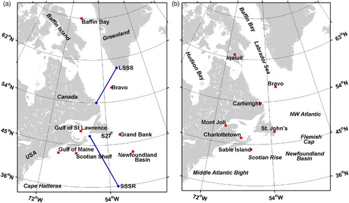
Finally, annual cycles of bidecadal monthly means, and annual-mean time series, of SAT, SST and SSS at selected sites (Fig. 1) in the historical and future RCP simulations were examined in more detail for five runs (Runs 1 to 5) of CanESM2 (chosen because of its usage in Canada; full model names can be found in Table 1) and Run 1 of GFDL-ESM2M, derived from monthly-mean data on their native grids (downloaded directly from the Canadian Centre for Climate Modelling and Analysis (CCCma) and GFDL data portals, respectively). The computations with the five-member CanESM2 ensemble allowed a brief examination of inter-run (or inter-member) variability (Loder and van der Baaren (2013) and Section 7a), for comparison with inter-model variability using Run 1 from the six ESMs. In all cases, model values at the selected sites were obtained using bilinear interpolation.

b Comparison with Observations

The observational realism of climate models is a limiting factor in their value for climate change projections. The exploratory comparisons of the historical simulations with observations included here are intended to provide an indication of how well the ESMs represent some key atmospheric, ice, and oceanic features in the NWA.

For SAT (whose spatial gradient across the land–ocean boundary is recognized to be coarsely represented in AOGCMs), annual cycles of bidecadal monthly means for the 1986–2005 period in the historical simulations of the six ESMs are compared with the corresponding observations from six meteorological stations (Fig. 1b) in the NWA region, using the Adjusted Homogenized Canadian Climate Dataset (AHCCD; Vincent et al., 2012) from Environment Canada (EC). In addition, interannual variability in SAT in the CanESM2 and GFDL-ESM2M historical simulations is compared with that observed since 1950 (Section 7a), using annual-mean time series from AHCCD and, for Bravo, from the National Centers for Environmental Prediction/National Center for Atmospheric Research (NCEP/NCAR) Reanalysis data (http://www.esrl.noaa.gov/psd/data/gridded/data.ncep.reanalysis.html).

For SIC, SST, SSS, and OML-max, the bidecadal monthly-mean spatial distributions in the six ESMs for 1986 to 2005 are compared with observational fields. For SIC, the observed monthly SIC distributions for 1986 to 2005 were computed from an updated version (http://www.metoffice.gov.uk/hadobs/hadisst) of the Hadley Centre Sea Ice and Sea Surface Temperature (HadISST1) dataset (Rayner et al., 2003). For SST, the monthly distributions from HadISST1 for 1986 to 2005 and observed monthly climatologies for the 10 m interval to 2002 were used, for representative cold (February) and warm (August) months. For SSS, the observed monthly climatologies for the 0–10 m interval, chosen to approximate the vertical smoothing associated with the 10 m surface layer in most of the models, were used. The 0–10 m climatologies were obtained using a multi-pass horizontal weighting and interpolation scheme to estimate monthly means on an initial 0.3° × 0.3° grid from available observations for 1946 to 2002 (see the Appendix for more details). These initial climatologies were further smoothed in order to have horizontal resolution closer to that of the interpolated ESM fields.

For the observational comparison with the ESMs’ bidecadal (1986–2005) OML-max for February, mixed-layer depths (MLDs) were estimated from all available individual Argo float profiles during the 2002–2014 period using a temperature change criterion of 0.15°C with a reference depth of 50 m, which is similar to that used by de Boyer Montégut, Madec, Fischer, Lazar, and Iudicone (2004) in their global climatology. Averages (over all years) of the highest 50% of the MLD values in 2° × 2° grid squares between mid-February and mid-March were used as approximations for OML-max because the data were too sparse to provide estimates of the OML-max for individual years.

For the observational bidecadal monthly means of SAT, SST, and SSS used in the annual-cycle comparisons, the standard deviation (SD_o) of the individual-year means about their bidecadal mean is included; in this case, the 95% statistical significance indicator is 2SE ≈ 0.4SD_o, assuming limited autocorrelation in the time series during the 1986–2005 period.

The 1986–2005 annual cycles of monthly SST and SSS in the interpolated historical data from the six ESMs, as well as the 1950–2012 annual-mean time series of SST and SSS in CanESM2 (five runs) and GFDL-ESM2M (one run), are compared with hydrographic profile observations from DFO's Atlantic Zone Monitoring Program (AZMP; http://www.bio.gc.ca/science/monitoring-monitorage/azmp-pmza-en.php) at two sites and its Atlantic Zone Off-shelf Monitoring Program (AZOMP; http://www.bio.gc.ca/science/monitoring-monitorage/azomp-pmzao/azomp-pmzao-en.php) at one site (Fig. 1a). The sites are Station 27 on the northern Grand Bank (∼47.5°N, 52.6°W; Colbourne et al., 2014), Emerald Basin on the central Scotian Shelf (∼44°N, 63°W; Hebert, Pettipas, Brickman, & Dever, 2014), and Bravo (∼56.5°N, 51°W; former location of the Ocean Weather Ship) in the central Labrador Sea where Argo profiles are also used (Yashayaev et al., 2014). From previous studies (e.g., Petrie, Loder, Akenhead, & Lazier, 1992; Umoh & Thompson, 1994; Yashayaev, 2007), the observations at these sites are expected to provide a reasonable representation of near-surface conditions over broader areas; time series from the nominal surface depth (0–5 m) are used for the first two sites and from the 10–30 m interval for Bravo in order to reduce aliasing of seasonal and vertical changes in the sparser data there.

For the vertical distributions of subsurface temperature and salinity across the LSSS section, the decadal means over the 1996–2005 period from the five ESMs are compared with observations for the 1996–2008 period from DFO's AZOMP and other sampling (e.g., Argo float profiles) on the AR7W line (e.g., Yashayaev et al., 2014).

c Projected Changes

The projected (60-year) climate changes from the ESMs were computed as the differences between the bidecadal monthly means for 2046 to 2065 from the RCP simulations and those for 1986 to 2005 from the historical simulations.

For a particular variable and season, there is substantial similarity between the spatial patterns of the projected changes for the two RCPs, and the differences between the ensemble-mean changes for the RCPs are generally less than the differences among the projected changes from the different models (Loder & van der Baaren, 2013). The similarity of the patterns for the two RCPs is not surprising considering that the climate system appears to have some fundamental modes of response to increased radiative forcing from GHGs (e.g., Ishizaki et al., 2012; Markovic et al., 2013). The limited differences in magnitude are not surprising considering the “committed” climate change during the next few decades that is associated with the increase in radiative forcing to date (e.g., Collins et al., 2013).

It is widely recognized in the climate science community that no single AOGCM or ESM is able to provide a robust representation of all the important processes in the climate system (e.g., Taylor et al., 2012), especially those affecting regional climate (e.g., Li, Zhang, Zwiers, & Wen, 2012; Shepherd, 2014). Consequently, IPCC projections are based on the statistics of an ensemble of models, numbering approximately 40 in AR5. Such an ensemble approach is also needed to represent regional climate change, perhaps even more so (e.g., Mearns et al., 2013). Although our subset of six ESMs is probably not representative of the CMIP5 AOGCMs in a broad statistical sense, we have nevertheless taken an ensemble approach in order to consider and take into account differences among the models. Examination of the inter-run variability of SAT and SST in the five-member ensemble of CanESM2 simulations (Loder & van der Baaren, 2013) indicated that there is little difference in the bidecadal means (e.g., annual cycles) from the different runs. Therefore, for the 60-year bidecadal climate changes, we only consider Run 1 from the six ESMs.

3 Surface air temperature

a Comparison with Observations at Selected Meteorological Stations

To provide an indication of the extent to which the annual cycles of SAT in the historical simulations are in agreement with observed air temperatures, Fig. 2 compares bidecadal monthly means for 1986–2005 from the AHCCD at six meteorological stations scattered across Atlantic Canada with those from the ESMs for the same period. Notable features include the large seasonal variation, the differences in the annual cycles among the sites, and the limited (4°–8°C, or approximately 20% of the annual range) spread among the annual cycles in the different ESMs except at the two northernmost sites (Iqaluit and Cartwright) where SAT in HadGEM2-ES is lower than in the other ESMs. The observed bidecadal means lie within or near the envelope of the model cycles and generally within the inter-model standard deviations (SD_m) of the ensemble-mean annual cycles (see Fig. 3-2b in Loder and van der Baaren (2013)). The observed and ensemble means are well within their combined observational (interannual; Fig. 2) and inter-model SEs of each other (0.4SD_o + 0.8SD_m). There are differences of a month in the timing of the annual minima and maxima among the models and between some models and observations, but there are only small differences in the timing of the extrema in the ensemble-mean and observed annual cycles (Loder & van der Baaren, 2013).

Fig. 2 Annual cycles of the bidecadal monthly means of SAT for 1986–2005 at six sites from observations (AHCCD, red; see Fig. 1b for locations) and from historical Run 1 of the six ESMs (see colour legend). The SD_o of the individual-year AHCCD monthly means about each bidecadal mean is indicated by the red error bar.

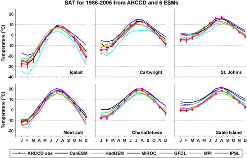
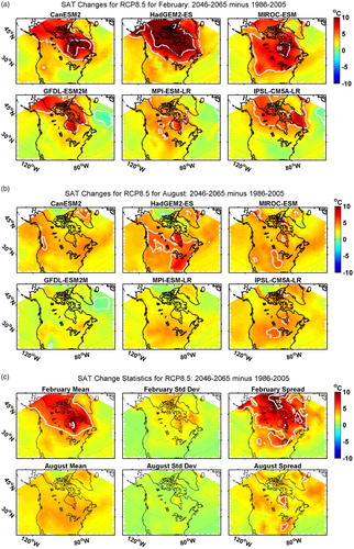
Fig. 3 Changes in bidecadal SAT for Canada from 1986–2005 to 2046–2065 from six ESMs for RCP8.5 in (a) February and (b) August. The ensemble mean, SD_m, and spread of the changes in (a) and (b) are shown in (c) for (top row) February and (bottom row) August. The white contours represent the 0°, 5°, and 10°C isotherms.

This comparison indicates that the ESMs have both a qualitative and reasonable quantitative representation of the large seasonal and broad spatial variation in bidecadal SAT over Atlantic Canada, although the SD_m is typically 2°–3°C (and larger in winter at the northernmost sites) and the differences between the ensemble and observed monthly means are typically 1°–4°C. Comparison of the time series of observed annual means (since 1950) with annual means from CanESM2 and GFDL-ESM2M at three sites (Section 7a) indicates that the observed interannual and decadal-scale SAT variability is not reproduced in the models, but this is as expected for AOGCM simulations initialized randomly about a century earlier (e.g., Taylor et al., 2012).

b Projected Changes

In this subsection, we focus on the projected climate changes in SAT from the six ESMs and their seasonal and spatial structure. We consider a Canada-wide domain in order to place the changes over the NWA in a larger-scale context. The patterns described below are similar to those in Diffenbaugh and Giorgi's (2012) examination of seasonal changes between 1986–2005 and 2080–2099 in a CMIP5 ensemble of 20 models.

Figures 3a and 3b show the projected changes in bidecadal mean SAT between 1986–2005 and 2046–2065 from each of the six ESMs for RCP8.5, for winter (February) and summer (August), and the ensemble statistics for the changes are presented in Fig. 3c. It is apparent that, over a large portion of the domain (including much of the NWA), the spread of the change estimates from the different models is comparable to (or exceeds) the ensemble mean of the changes, particularly in winter, pointing to uncertainty in their regional climate change projections. However, in general, the SD_m is substantially smaller than the magnitude of the ensemble-mean change, such that a confidence interval based on two SEs (≈0.8SD_m) would point to SAT increases that are significantly different from zero in most areas. The comparable magnitudes of the SD_m values for the historical and future ensemble means (Loder & van der Baaren, 2013) suggest that the inter-model differences in the change fields are related to inter-model differences in both the historical and future simulations.

The winter change pattern in all six ESMs (Fig. 3a) shows a broad (warming) maximum of Arctic amplification (e.g., Serreze & Barry, 2011) over northern central Canada but with substantial inter-model variability (by a factor of two) in its extent, shape, and magnitude. For Atlantic Canada and the NWA, some models show the largest increases extending southeastward from northern central Canada while others show the largest increases over the northern Labrador Sea and/or Hudson Bay (pointing to a possible regional sea-ice influence on the change patterns). In some models there is a suggestion of a tail of larger increases extending eastward from the continent across the southern part of Atlantic Canada and the NWA and, in most models, an area of smaller increases (with decreases in two models) in the northern North Atlantic southeast of Greenland consistent with IPCC AR4 and AR5 (e.g., Collins et al., 2013; Meehl et al., 2007).

The summer change pattern in all six ESMs (Fig. 3b) shows a weaker broad (warming) maximum at mid-latitudes over the North American continent, again similar to AR4 and AR5, with substantial inter-model variability in extent, shape, and magnitude (by a factor of two). A clear feature in five of the ESMs is the eastward extension of a zonal band of enhanced increases across southern Atlantic Canada and the NWA that is more pronounced than in winter. Possible contributing factors to this band are offshore advection of the mid-latitude continental maximum and northward expansion of the North Atlantic's subtropical ocean gyre (Sections 5a and 7b).

The ensemble-mean 60-year SAT increases in February (for RCP8.5) are greater than 3°C over almost all of Canada and its adjacent waters (Fig. 3c). The increases exceed 5°C north of 50°–55°N and peak at 10°C over Hudson Bay. Over Atlantic Canada and the NWA, the (ensemble-mean) increases range from about 2°–3°C in the south and east to 6°–8°C in the north. In August, the increases range from approximately 4°C over southern Canada to approximately 1°C over the Arctic Ocean, with increases over Atlantic Canada and the NWA in the 2°–3°C range.

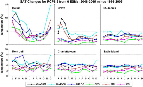
The 60-year monthly changes in SAT at five of the meteorological sites and at Bravo are shown in Fig. 4 for the individual ESMs. For the four southernmost sites (south of 50°N), the increases are approximately the same year-round although the inter-model differences are comparable in magnitude to the ensemble-mean changes (Loder & van der Baaren, 2013). There is some indication of weak winter and summer maxima at these sites, reflecting the different winter and summer spatial patterns discussed above (Fig. 3), but the amplitude of the seasonal variation in the ensemble means is much less than the SD_m values (Loder & van der Baaren, 2013). In contrast to the southern sites, there is a seasonal variation in the increases at the two northernmost sites (Iqaluit and Bravo), with the largest magnitudes occurring in February (consistent with Fig. 3) and weak minima in May (Bravo) and September (both sites). The winter–summer differences exceed the SD_m values at Iqaluit (and Cartwright, not shown), but not at Bravo (Loder & van der Baaren, 2013). In summary, increased SAT is projected over all of Atlantic Canada and most of the NWA on the 60-year time scale, but there is strong spatial structure and substantial uncertainty in its magnitude, particularly in winter.

Fig. 4 Changes in bidecadal monthly SAT from 1986–2005 to 2046–2065 for RCP8.5 at six locations (shown in Fig. 1b) from Run 1 of the six ESMs.

4 Sea-ice concentration

In this section we briefly examine the distributions of one metric of sea-ice variability, namely the sea-ice area fraction or SIC expressed as a percentage. The goal is as much to obtain an indication of the realism of the representation of sea-ice variability in the ESMs affecting air–sea interactions and ocean properties, as to obtain specific projections for SIC changes. Studies of sea-ice variability in the Arctic Ocean using the CMIP5 models have been published with particular focus on the observed and expected reductions in summer ice cover and volume (e.g., Stroeve et al., 2012; Wang & Overland, 2012). However, limited attention has been given to the representation of sea-ice variability in the NWA in the CMIP3 and CMIP5 models, although some climate change simulations for the Canadian Arctic Archipelago using ice–ocean models have been reported (Hu & Myers, 2014; Sou & Flato, 2009).

a Comparison with Observed Spatial Distributions

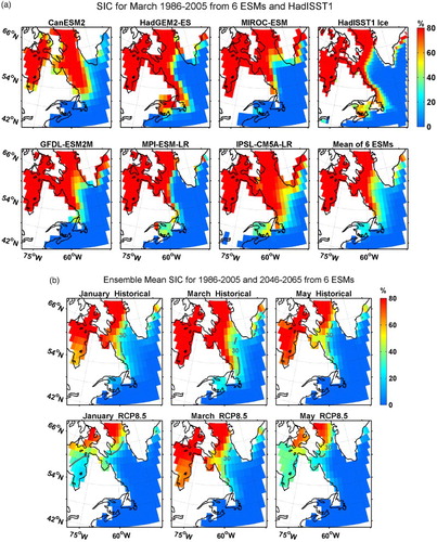
Figure 5a shows the bidecadal SIC distributions from the historical simulations of the six ESMs, their ensemble mean, and the HadISST1 observations for March, which approximates the seasonal maximum of sea ice in the eastern Arctic and NWA. On a broad scale, all of the models show the approximate southward extent of sea ice to approximately 50°N in March and the retreat to the vicinity of northern Baffin Bay and the Arctic Archipelago in September (see Loder & van der Baaren, 2013). However, if the spatial pattern and seasonal timing of sea-ice cover between Baffin Bay and the Gulf of St. Lawrence is examined in more detail (see Fig. 1 for locations), significant differences among the models and between the models and observations are apparent. As examples, only three of the models (HadGEM2-ES, IPSL-CM5A-LR and MPI-ESM-LR) have winter ice cover occurring in the Gulf of St. Lawrence as observed; all the models have greater March ice cover in the Labrador Sea than observed, by a substantial amount in some cases (e.g., CanESM2 and IPSL-CM5A-LR), and the springtime (April–May) extension of ice cover to the Grand Bank is not reproduced in any of the models (Loder & van der Baaren, 2013). This lack of agreement is actually not surprising considering the relatively coarse spatial resolution of the ice and ocean models in the region compared with the scales of important ocean features, such as the straits connecting the Arctic and NWA oceans, as well as the width of the Labrador Current (e.g., Cooke, Demirov, & Zhu, 2014; Wang, Myers, Hu, & Bush, 2012). Nevertheless, it raises questions about the adequacy of the regional representation of air–sea fluxes and meltwater (with implications for SST, SSS, and other variables) in the ESMs.

Fig. 5 (a) Comparison of SIC in March from the historical simulation (1986–2005) of each of six ESMs, the HadISST1 dataset for 1986–2005 (upper right), and the ensemble mean from the ESMs (only shown for grid points with values from all six ESMs). The differences in the apparent land areas (white) in the different models largely reflect differences in their native grids. (b) Ensemble-mean bidecadal monthly SIC for (left) January, (middle) March, and (right) May for 1986–2005 from (upper) the historical simulations and (lower) for 2046–2065 for RCP8.5 from the six ESMs (only shown for grid points with values from at least three ESMs). The grey contour in (b) represents the 30% isoline, approximating the ice edge.

b Projected Changes

The ensemble-mean bidecadal SIC fields in January, March, and May for the 1986–2005 period (from the historical simulations) and for the 2046–2065 period (for RCP8.5) are shown in Fig. 5b, indicating the overall winter–spring evolution of SIC in the ESMs. While the detailed SIC patterns differ in the various models, there is a clear future reduction in the equatorward extent of sea ice in both seasons in all of the models (Loder & van der Baaren, 2013). This general feature of reduced SIC in the NWA is consistent with observations of an overall decline in sea-ice extent in the region over the past half century (e.g., Cavalieri & Parkinson, 2012; Peterson & Pettipas, 2013; Tivy et al., 2011) and the ice–ocean model simulations of future change (Hu & Myers, 2014; Sou & Flato, 2009). Although it appears that the exact locations and spatial extent of the areas of the reduction in SIC in the present models, as well as the magnitude of the reductions, are not reliable, there is an indication in the projections that, for some months, some sub-regions such as the Gulf of St. Lawrence and Hudson Bay (e.g., Joly, Senneville, Caya, & Saucier, 2011) could change from largely to barely (if at all) ice covered over the next 60 years. Also, there is a substantial reduction in SIC in the Labrador Sea in winter in the model projections that, even if not realistic in magnitude because the historical SIC is overestimated, probably has a substantial influence on the projected SAT and SST changes (e.g., Jahn & Holland, 2013; Markovic et al., 2013).

5 Ocean temperature and salinity

In this section we examine the spatial and temporal variability of ocean temperature and salinity in the ESMs, focusing on the NWA and starting with SST and SSS.

a Sea Surface Temperature

1 Comparison with observed spatial and temporal variability

Figure 6 shows the bidecadal mean distributions of SST for February 1986–2005 from the historical simulations, together with the observed SST from HadISST1 for 1986–2005 and a smoothed version of the 0–10 m temperature climatology for 1946–2002 for the same month. There is qualitative and some quantitative similarity among the modelled and observed fields in the large-scale contrast (∼20°–25°C) of subpolar and subtropical waters in the NWA (e.g., Loder et al., 1998) and in the seasonal change (∼10°–15°C; Fig. 7) from winter to summer (see Loder and van der Baaren (2013) for the corresponding August fields). However, there are notable differences among the models and observations in the spatial structure of the important subpolar-subtropical water boundary. In particular, the separation position of the Gulf Stream from the shelf edge (illustrated by the 18°C isotherm) is too far north in all the models compared with its observed position off Cape Hatteras, and the North Atlantic Current (illustrated by the 10°C isotherm) does not extend far enough north to the east of Flemish Cap in five of the models (with GFDL-ESM2M being the exception). This results in water of subtropical origin extending too far north to the west of the Grand Bank and not far enough north to the northeast of Flemish Cap. This can alternatively be described as water of subpolar origin generally not extending far enough equatorward along the east coast of North America and extending too far eastward in the offshore North Atlantic north of Flemish Cap. There are similar discrepancies in summer, with warm water of subtropical origin extending too far north towards the Gulf of Maine and Scotian Shelf and cool water of subpolar origin not extending far enough south onto the Grand Bank in the ESMs (Loder & van der Baaren, 2013).

Fig. 6 Comparison of SST in February from the historical simulation of each of six ESMs for 1986–2005, the HadISST1 dataset for 1986–2005 (upper right), and the observed 0–10 m temperature climatology for 1946–2002 smoothed over an approximate 2° scale (for comparable resolution to the ESMs). The white contours represent the 2°, 10°, and 18°C isotherms.

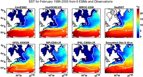
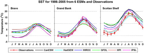
Fig. 7 Annual cycles of SST at the three DFO monitoring sites from observations (red; see Fig. 1a for locations) and for 1986–2005 from historical Run 1 of the six ESMs (see colour legend). The observed annual cycle for Bravo is from a harmonic fit to data over all years with an overall SD_o of 0.9°C (not shown on plot), and the cycles for the other sites are from monthly means for 1986–2005 with each vertical (red) bar indicating the SD_o of the individual-year means about the bidecadal mean.

The ESMs’ difficulty in reproducing the position of the Gulf Stream is not surprising considering their typical 50–150 km ocean grid size and previous ocean model sensitivity studies that point to the importance of high resolution, low dissipation, and (advective) ocean heat flux convergence in resolving its separation position and recirculation (e.g., Bryan, Hecht, & Smith, 2007; Dewar, 2001). The misrepresentation of the position of the North Atlantic Current is similar to that described by van Oldenburgh et al. (2009) in CMIP3 models (also see Jungclaus et al. (2013) for a discussion of these ocean circulation features in one of the ESMs).

Figure 7 compares the seasonal variation in SST during the 1986–2005 period in the ESM historical simulations with the observed near-surface temperature annual cycles at the three DFO monitoring sites. At Bravo, four of the ESMs have means and annual cycles similar to those observed, while the other two (CanESM2 and IPSL-CM5A-LR) have substantially lower (by ∼4°C) winter values than observed. On the Grand Bank, the amplitude of the annual cycle is smaller than observed in five of the ESMs and slightly larger than observed in one, with winter SSTs in the models higher than observed and summer SSTs generally lower than observed. On the Scotian Shelf, winter SSTs in all the models are higher than observed in winter, in some (e.g., CanESM2 and GFDL-ESM2M) by more than 5°C, whereas summer SSTs in the different models bracket the observations. The differences between the ensemble monthly means from the ESMs (Loder & van der Baaren, 2013) and the observed means are generally less than the combined SEs (0.4SD_o + 8SD_m), except on the Scotian Shelf in winter, pointing to approximate agreement except in the subpolar-subtropical transition zone.

Comparison of the time series of annual-mean SSTs in the historical simulations of CanESM2 and GFDL-ESM2M with the observed annual means (for 1950–2012) at these same sites (Section 7a) confirms that the observed interannual and decadal-scale SST variability is not reproduced in the models, as expected (e.g., Taylor et al., 2012).

2 Spatial distribution of projected changes

The 60-year SST change fields in February and August for RCP8.5 in Figs 8a and 8b show the magnitudes and spatial patterns in winter and summer. Notable general features include i) the substantial spatial structure with latitudinal gradients; ii) the differences in the patterns among the models; iii) warming in most areas but also areas with cooling, particularly in winter; and iv) the greater overall warming in summer than winter. There is an overall tendency for a mid-latitude zonal band of greater warming, with the largest magnitude occurring in summer, extending eastward from the Scotian Shelf. There is considerable similarity in this band in three models in winter and in four models in summer. Candidate contributors to this band include a poleward expansion of or shift in the subtropical gyre in the models (e.g., Saenko, Fyfe, & England, 2005; Wu et al., 2012) and the band of enhanced SAT warming extending eastward over the region (Fig. 3).

Fig. 8 Changes in bidecadal monthly SST from 1986–2005 to 2046–2065 for the NWA for RCP8.5 from the six ESMs (first three columns) for (a) February and (b) August. The ensemble mean, SD_o, and spread of the changes are also shown (last two columns) for grid points with values from at least three ESMs. The white contours represent the −4°, 0°, and 4°C isotherms.

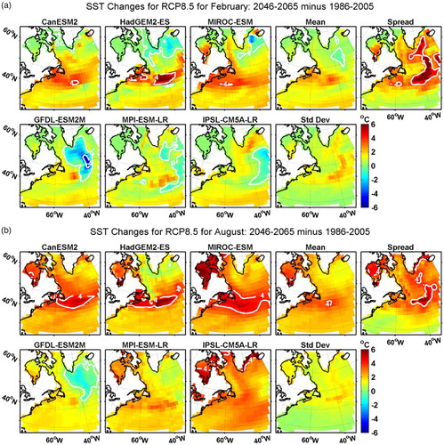
There is also a general tendency for limited warming in northern areas in winter (Fig. 8a), which is consistent with continued sea-ice cover (Fig. 5). However, there is wide variation in the summer changes among the models in these areas (Fig. 8b) that is probably related to their different spring sea-ice cover. All the models have an area of cooling or substantially reduced warming south or southeast of Greenland, similar to that in AR4 and AR5 and often attributed to a reduction in the AMOC (e.g., Collins et al., 2013; Drijfhout et al., 2012), although a change in the advection of subtropical water into the subpolar gyre may also be a factor. On the sub-basin (e.g., subpolar, subtropical, and mid-latitude transition zone) and sub-regional (e.g., Labrador Shelf, Grand Bank, and Scotian Shelf) scales (see Annex 1 of Brock, Kenchington, and Martinez-Arroyo (2012) for context), there are similarities in the change patterns across most of the models but also differences such that the reliability of the specific projections from any particular model is unclear.

The ensemble statistics for the SST changes are included in Fig. 8. For a particular season, there is close similarity in the patterns of the statistics for RCP4.5 and RCP8.5 (Loder & van der Baaren, 2013), with slightly greater mean warming for RCP8.5, particularly in August. The amplified warming in August (3°–4°C at mid-latitudes) is consistent with much of the spring–summer surface heat input being trapped in the shallow spring–summer mixed layer. The spread of the SST changes among the models is noticeably larger than the magnitude of the ensemble-mean changes, in contrast to the situation for SAT (Fig. 3c) for which the spread and the mean are comparable. The SD_m values for the SST changes are also larger (than those for the SAT changes) relative to the ensemble means, with comparable magnitudes to the mean changes in winter in some areas.

Considering the spread among the different ESMs and the simulations for both RCP4.5 and RCP8.5, the 60-year changes in winter SST for the shelf sub-regions off Atlantic Canada are projected to be in the range of 0°–1°C for the northern Labrador Shelf, 0°–2°C from the central Labrador Shelf to Flemish Cap, 1°–3°C for the Grand Bank and southern Newfoundland Shelf, and 1°–4°C for the Gulf of St. Lawrence, Scotian Shelf, and Gulf of Maine (see Loder and van der Baaren (2013) for more detail). In summer, the corresponding changes are in the range of 1°–3°C for the northern Labrador Shelf; 0°–3°C for the central Labrador Shelf and northeast Newfoundland Shelf; 1°–4°C for the Grand Bank, western Scotian Shelf, and Gulf of Maine; and 1°–5°C for the Gulf of St. Lawrence, southern Newfoundland Shelf, and central Scotian Shelf.

3 Temporal variability of projected changes

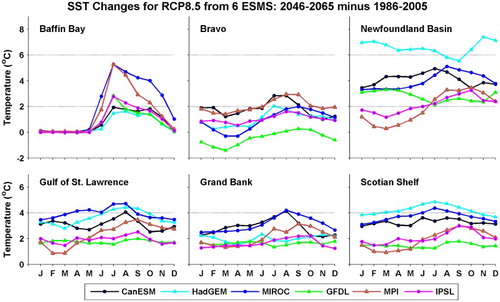
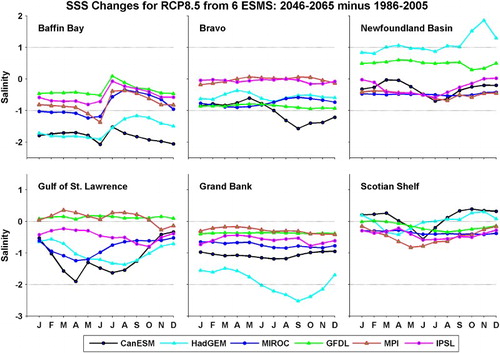
The ensemble bidecadal monthly means of SST for 1986–2005 (historical) and 2046–2065 (RCP8.5) at nine sites off Atlantic Canada are within their combined SD_m values for all months and sites (see Figs 5-9a of Loder and van der Baaren (2013)), reflecting the modest magnitude of the climate changes relative to the model uncertainties. The inter-model and seasonal variability in the climate changes is apparent in the monthly SST changes for the individual ESMs at six of these sites (Fig. 9). The inter-model spreads of the changes are typically in the 2°–4°C range at most sites, with the notable exceptions of Baffin Bay where there are no changes in winter (associated with continued sea-ice cover), the Newfoundland Basin where the spreads are 3°–6°C (associated with a 7°C increase in one model (HadGEM2-ES in winter)), and the Grand Bank where the spreads in winter are < 2°C (probably related to the influence of upstream sea ice). At the Baffin Bay and Bravo sites, there is a qualitatively consistent seasonal variation in the magnitude of the changes across all the models, whereas at the other sites the variation is consistent across only some of the models. At all sites except Baffin Bay, the seasonal variation of the ensemble-mean changes is smaller than or comparable to the inter-model SD_m values (Loder & van der Baaren, 2013). There are, however, indications in most models of larger increases in summer than winter at most sites, consistent with the broadscale differences between the February and August mean change fields in Fig. 8.

Fig. 9 Changes in bidecadal monthly SST from 1986–2005 (historical) to 2046–2065 (RCP8.5) at six sites in Fig. 1a for Run 1 of the six ESMs.

The projected future evolution of annual-mean SST in CanESM2 and GFDL-ESM2M for RCP8.5 at the three DFO monitoring sites is discussed in Section 7a.

b Sea Surface Salinity

In this subsection we examine the spatial and temporal variability of SSS in the ESMs, in an analogous approach to that for SST in the preceding section.

1 Comparison with observed spatial and temporal variability

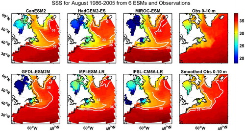
Figure 10 shows the bidecadal mean SSS distributions in the six ESMs for August during 1986–2005, together with two versions of the observed 0–10 m August climatology for 1946–2002, one on its original 0.3° × 0.3° grid and the other smoothed to have comparable resolution to the ESMs. The corresponding offshore model distributions for February are similar, reflecting the limited seasonal variation except in coastal areas (Loder & van der Baaren, 2013). Similarities in the broadscale SSS patterns among the different models and observations can be seen, especially for the mid-latitude transition zone from the relatively fresh subpolar (and continental run-off) waters to water of subtropical origin. However, similar to SST, there are notable differences both among the models and with the observations. In particular, high-salinity water of subtropical origin (S > 35 in Fig. 10) extends too far north in the Middle Atlantic Bight and Gulf of Maine region in all six ESMs and low-salinity subpolar-origin water extends (S < 33) too far east in the Grand Bank region in five of them (with GFDL-ESM2M being the exception, as found earlier with SST). In addition, there are differences in more northerly areas and in Hudson Bay in particular. The differences in the northward extent of water of subtropical origin reinforce the concerns based on SST regarding the detailed boundary of the subtropical and subpolar gyres in the ESMs, whereas the differences in the LSSS region reinforce the concerns based on SIC regarding the extent of sub-Arctic meltwater in the northern part of the NWA.

Fig. 10 Comparison of SSS in August from the historical simulation of each of six ESMs for 1986–2005, the observed 0–10 m salinity climatology for 1946–2002 on a 0.3° × 0.3° grid, and the climatology smoothed over an approximate 2° scale. The white contours represent the 33 and 35 isohalines.

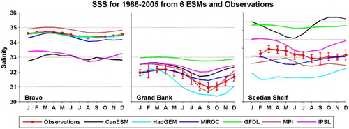
The observational comparison for the bidecadal annual cycles from the six ESMs at the three DFO monitoring sites is shown in Fig. 11. One striking feature of the comparison is the substantially larger variability in mean SSS among the models at the Scotian Shelf site in the subpolar-subtropical transition zone than at the Bravo and Grand Bank sites in the subpolar region. This reflects the previously discussed difficulty of resolving the subpolar-subtropical boundary in the models. At Bravo, the seasonal variation in all the ESMs shows some similarity to the weak variation observed, and four of the ESMs are in approximate agreement with the observed mean SSS. However, the SSS in the other two (CanESM2 and IPSL-CM5A-LR) is low by about 2, which is a significant amount from the perspective of the important role of salinity in deep convection in the Labrador Sea (e.g., Yashayaev, 2007). On the Grand Bank, there is also similarity in the phase of the seasonal variation among the models and observations, but there is substantial spread in the variation's amplitude (∼1) and in the annual mean (∼1.5) compared with those observed (with the means in CanESM2 and GFDL-ESM2M high by > 1 and those in HadGEM2-ES low by >1). In contrast, there is little similarity among the amplitude and phase of the modelled and observed seasonal variations at the Scotian Shelf site, and there is a wide spread (∼3) in the ESMs’ annual means around that observed. Nevertheless, the observed and ensemble means are within their combined SEs (0.4SD_o + 0.8SD_m) in all months at all three sites (Loder & van der Baaren, 2013), but this should be interpreted with caution in view of the above discrepancies and the complexity of the region.

Fig. 11 Annual cycles of SSS at the three DFO monitoring sites from observations (red) and for 1986–2005 from historical Run 1 of the six ESMs. The observed annual cycle for Bravo is from a harmonic fit to data over all years with an overall SD_o of 0.2, and the cycles for the other sites are from monthly means for 1986–2005 with each vertical (red) bar indicating the SD_o of the individual-year means about the bidecadal mean.

The time series of the observed SSS annual means at the three sites during 1950–2012, as well as those from the five CanESM2 runs and Run 1 of GFDL-ESM2M, show pronounced differences and only weak or insignificant correlations in the interannual-to-decadal variability among the observations, runs and models (see Fig. 6-4 in Loder and van der Baaren (2013)). The long-term trends in both the models and observations are weak compared with this variability, consistent with the strong interannual to multi-decadal variability observed in the NWA (Bindoff et al., 2007; Durack & Wijffels, 2010; Reid & Valdés, 2011; Yashayaev, 2007).

2 Spatial distribution of projected changes

The projected 60-year changes for August and RCP8.5 are shown in Fig. 12. Unlike those for SST, there is little seasonal variation in the SSS change patterns (Loder & van der Baaren, 2013). A clear broadscale pattern is apparent, with decreasing SSS in the subpolar and mid-latitude transition regions (north of about 40°N) and increasing SSS in the waters of subtropical origin to the south. This pattern is consistent with expectations from the CMIP3 and CMIP5 models (Capotondi, Alexander, Bond, Curchitser, & Scott, 2012; Durack, Wijffels, & Matear, 2012; Meehl et al., 2007) that also show freshening associated with the intensified hydrological cycle and ice melt in the north and increasing salinity associated with increased evaporation in areas under subtropical influences. However, as with the projected SST changes, there are substantial differences among the ESMs in the detailed spatial structure of the changes.

Fig. 12 Changes in bidecadal monthly SSS from 1986–2005 to 2046–2065 for RCP8.5 for August from the six ESMs (first three columns). The ensemble mean, SD_m, and spread of the changes are also shown for grid points with values from at least three ESMs. The grey contour represents the 0 isohaline.

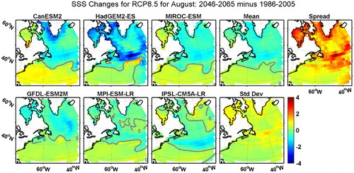
The ensemble statistics for these SSS changes are included in Fig. 12. The boundary for the latitudinal change in sign (0 isohaline) of the ensemble-mean changes lies around 40°N. There is an associated zonal band of enhanced inter-model spread (in the 1–3 range) extending across the North Atlantic in the vicinity of the subtropical-subpolar gyre boundary, reflecting the ESMs’ differences in the representation of this important feature. The largest decreases (in the open NWA) in the ensemble mean are in a zonal band at approximately 45°N, east of the Grand Bank, with a magnitude of approximately 1, while the largest increases are less than 1 in the subtropical gyre to the south. All of the ESMs show a decrease in SSS along the Labrador and Newfoundland Shelves in both winter and summer (Loder & van der Baaren, 2013), but the sign of the (small) changes on the Scotian Shelf and in the Gulf of Maine depends on the model and season.

3 Temporal variability of projected changes

The ensemble bidecadal monthly means of SSS at the nine sites off Atlantic Canada (see Fig. 6-9a in Loder and van der Baaren (2013)) show a decrease from 1986–2005 to 2046–2065 at all sites in all months, except in the south at the Gulf of Maine, Scotian Shelf, and off-shelf Newfoundland Basin and Scotian Rise sites where there are small increases in some months. However, in all cases, the mean changes are less than the combined inter-model SEs (of the bidecadal means), reflecting the model uncertainties.

The seasonal variations of the 60-year SSS changes in the individual ESMs at six sites are shown in Fig. 13. The seasonal variations are small relative to the inter-model differences, with the most consistent changes across models occurring in Baffin Bay where there is an enhanced decrease in SSS in May and June followed by a smaller decrease (or slight increase) in July and August (probably related to the end of the sea-ice season there).

Fig. 13 Changes in bidecadal monthly SSS from 1986–2005 (historical) to 2046–2065 (RCP8.5) at six sites shown in Fig. 1a, in Run 1 from the six ESMs.

The projected future evolution of the annual SSS means from CanESM2 and GFDL-ESM2M at the three DFO sites indicates clear differences in the nature and magnitude of the variability among those models and sites, as well as differences in the interannual-to-decadal variability among the CanESM2 runs (see Fig. 6-10 of Loder and van der Baaren (2013)), further indicating uncertainty in future SSS in the NWA.

c Cross-Basin Structure of Ocean Temperature and Salinity

In this subsection, we examine annual-mean subsurface temperature and salinity from five of the ESMs on vertical sections across the LSSS and the SSSR (see Fig. 1a for their locations).

1 Comparison with observations

We start by comparing the modelled decadal-mean temperature and salinity across the LSSS during 1996–2005 (Fig. 14) with observed distributions on the nearby AR7W line (Yashayaev et al., 2014).

Fig. 14 Comparison of decadal means (1996–2005) of (a) potential temperature and (b) salinity across the LSSS section from five ESMs, with observations from the AR7W line over the period 1996–2008 (data from Yashayaev et al., 2014).

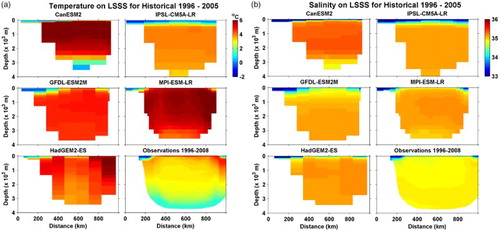
All the ESMs include a crude representation of the relatively cool and fresh water over the Labrador Shelf, but the extent of this layer across the Labrador Sea varies among the models, with it extending completely across in one of the models (IPSL-CM5A-LR). The offshore intermediate-layer water is too warm and salty in all of the models but by significantly varying amounts. The CanESM2 and MPI-ESM-LR models produce the largest overestimation of temperature at intermediate depths and CanESM2 produces the largest overestimation of salinity. This points to a poor representation of Labrador Sea Water that is formed in this region by wintertime convection (Yashayaev, 2007; Yashayaev & Loder, 2009), reminiscent of de Jong, Drijfhout, Hazeleger, van Aken, and Severijns (2009) findings for the AR4 models. The deep waters in the ESMs are also too warm and salty in general (also similar to the findings of de Jong et al.), with the exception of the bottom water being too cold in CanESM2.

2 Projected changes

The projected changes in bidecadal mean temperature and salinity from 1986–2005 to 2046–2065 in the five ESMs on the LSSS section are shown in Fig. 15 and those for the SSSR section in Fig. 16 (see Loder and van der Baaren (2013) for a discussion of the bidecadal mean SSSR fields).

Fig. 15 Changes in bidecadal means of (a) potential temperature and (b) salinity from 1986–2005 (historical) to 2046–2065 (RCP8.5) on the LSSS section from five ESMs, with the 0 isolines shown in grey.

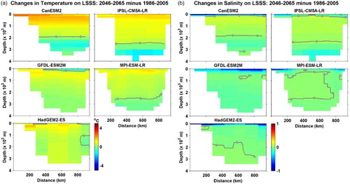
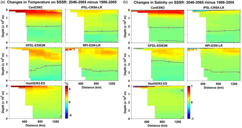
Fig. 16 Changes in bidecadal means of (a) potential temperature and (b) salinity from 1986–2005 (historical) to 2046–2065 (RCP8.5) on the SSSR section from five ESMs, with the 0 isolines shown in grey.

Warming by differing amounts with somewhat different spatial patterns is apparent in the temperature change fields in Figs 15a and 16a. The greatest warming on the LSSS section is in CanESM2 on the Labrador Shelf (>2°C) and decreasing offshore in the upper 800 m across the Labrador Sea, whereas the greatest warming on the SSSR section is in CanESM2 and HadGEM2-ES on the Scotian Shelf (>4°C) and decreasing offshore in the upper 200–600 m. On the other hand, there are small (<0.5°C) decreases in near-surface temperature in parts of the Labrador Sea in GFDL-ESM2M and HadGEM2-ES, with those in the former extending to approximately 200 m and small decreases in temperature at depth (>2000 m) on the LSSS section in three models and on the SSSR section in four models. Overall, warming is projected to a depth of at least 2000 m on both sections in the ESMs, which is at least qualitatively consistent with the ocean's established role as a major heat reservoir and important regulator of the Earth's climate system (e.g., Levitus et al., 2012; Stocker et al., 2013).

The projected salinity changes on the two sections are in contrast to the temperature changes in that they have greater variability in sign, in addition to differing magnitudes in the different models and on the two sections. On the LSSS section there is a decrease in near-surface salinity in all of the models. However, in only two models (GFDL-ESM2M and HadGEM2-ES) do the decreases extend to the intermediate waters (>500 m) over most of section, while in two others (CanESM2 and IPSL-CM5A-LR) there are widespread salinity increases below the upper 200–300 m. Thus, although all the models show the subpolar surface freshening expected from ice melt and the intensified hydrological cycle, there are indications of differing circulation or upstream water mass changes affecting subsurface salinity. On the SSSR section, there is a broad pattern of surface freshening in a thin layer (<100–200 m) in all the models extending offshore from the Scotian Shelf and of increasing salinity in the remainder of the upper 2000–3000 m with the largest magnitudes being in the upper 500–1000 m consistent with the northward expansion of the subtropical gyre. Below 2000 m there is weak freshening in four models. These patterns are broadly consistent with the anticipated competition between subpolar surface freshening and subtropical salinification and expansion in the North Atlantic's confluence/transition zone (e.g., Capotondi et al., 2012; Meehl et al., 2007; Palmer, Good, Haines, Rayner, & Stott, 2009), but the inter-model differences reflect the challenges in reproducing the ocean dynamics and thermodynamics in this complex region.

6 Ocean mixed-layer depth

In this section we examine the maximum depth of OML-max in winter in the four ESMs for which data were available. Figure 17a presents the spatial distribution of OML-max for February from 1986 to 2005 (historical) and from 2046 to 2065 (RCP8.5), together with a representation of the observed late-winter OML-max climatology from 2002 to 2014. There is a common coarse-scale pattern across the historical model fields and the observed climatology, with enhanced MLDs (>200 m) in a mid-latitude band extending eastward from the Middle Atlantic Bight in the Gulf Stream region (possibly related to the observed subtropical mode water referred to as “Eighteen Degree Water”; Talley & Raymer, 1982) and more localized areas with much larger enhancements in the subpolar region (consistent with its well-known deep convection; e.g., de Boyer Montégut et al., 2004; Våge et al., 2009; Yashayaev, 2007). There are also important differences among the models and observed climatologies (also see de Boyer Montégut et al., 2004). In three models, the mid-latitude and subpolar areas with enhanced mixed layers are not connected, whereas they are in GFDL-ESM2M and in the climatologies. There are large differences in the magnitudes and spatial structure of the enhanced subpolar MLDs among the models and climatologies. There is no deep (>500 m) convection in the Labrador Sea in two models (CanESM2 and IPSL-CM5A-LR) and only a small area of convection to 1000 m in the southern Labrador Sea in a third (GFDL-ESM2M), such that intermediate-depth water mass modification in the Labrador Sea in these models is much less than observed (as in earlier versions of these models; de Jong, Drijfhout, Hazeleger, van Aken, & Severijns, 2009). In contrast, in MPI-ESM-LR, there is a large area of deep mixed layers that extend to the bottom (2800 m) in some locations, which is much broader and deeper than observed. These poor representations of deep convection in the subpolar NWA are probably interrelated with those described earlier for sea-ice coverage (too much in the Labrador Sea) and the subtropical-subpolar gyre boundary (not far enough north to the east of Flemish Cap) and may be particularly significant in their influences on the globally important AMOC.

Fig. 17 (a) Bidecadal mean fields of OML-max in February from four ESMs for 1986–2005 from their historical simulations (top row) and for 2046–2065 from their RCP8.5 simulations (bottom row). The right panel in the top row shows an observational approximation to OML-max in February from Argo profiles during the 2002–2014 period. (b) Projected changes from 1986–2005 to 2046–2065 for the ESM fields in (a), with the 0 isoline shown in grey.

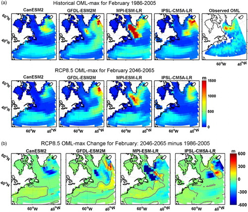
The OML-max fields for February 2046–2065 (Fig. 17a) show similar patterns to those for 1986–2005, with a reduction in the magnitude and extent of the large values in the subpolar areas apparent. The projected changes in OML-max are best seen in the change fields between these periods (Fig. 17b). There are substantial (by >200 m) reductions in OML-max in the subpolar areas with deep mixed layers, as well as patches with substantial increases in OML-max at the fringes of these areas. The former is expected with surface warming and freshening, whereas the latter probably reflects changes in ocean circulation of uncertain reliability (and slight horizontal shifts of the water with deep mixed layers). There is also a broad area with small (<100 m) increases in OML-max in the area of the enhanced depths extending eastward from the Middle Atlantic Bight to beyond the Grand Bank in three of the models. These increases are probably related to some combination of changes in the position and structure of the gyre-gyre boundary and the Eighteen Degree Water. Considering the discrepancies between the model and observed distributions of OML-max discussed in relation to Fig. 17a, the projected changes from these ESMs should be interpreted with caution, except for the general reduction in MLDs in the subpolar deep convection areas, which is consistent with expectations (e.g., Collins et al., 2013).

7 Air–sea variability and linkages

In this section we follow up on some issues arising from the results presented above.

a Inter-Run, Inter-Model, and Interannual-to-Decadal Variability

As part of this study, the seasonal and interannual variabilities in SAT and SST among Runs 1–5 of CanESM2 and Run 1 of GFDL-ESM2M for the historical, RCP4.5, and RCP8.5 simulations were compared for selected sites. The SST changes for the Bravo, Grand Bank, and Scotian Shelf sites (Fig. 1a), together with SAT changes at (collocated or nearby) Bravo, St. John's, and Sable Island (Fig. 1b), were examined in conjunction with consideration of the ensemble change statistics for the six ESMs in Figs 3 and 8. The inter-run SDs of SAT for the bidecadal (1986–2005) monthly means (in CanESM2) were found to be much less (<25%) than the corresponding inter-model SD_m values of SAT (using Run 1 from each ESM), whereas the inter-run SDs of SST were found to be much less than the inter-model SD_m values of SST. The inter-run SDs of both the SAT and SST changes (from 1986–2005 to 2046–2065) were found to be substantially smaller (although not much less) than the corresponding inter-model SD_m values of these respective changes. These relative magnitudes point to more variability in SAT and SST among the different ESMs examined than among the different members of CanESM2, which suggests that examination of multiple AOGCMs should be given priority over the examination of multiple runs (of the same AOGCM) in projecting climate changes in the NWA.

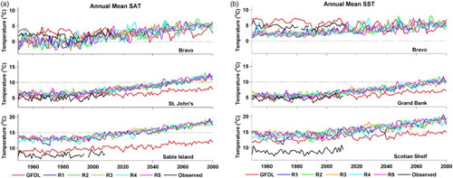
The time series of annual-mean SAT for the 1950–2080 period (historical and RCP8.5) for the five CanESM2 runs are noticeably different from each other (Fig. 18a) and very different from those for GFDL-ESM2M, with none having the same interannual-to-decadal variability as observed (with no, or only weakly, significant correlations after detrending). Similarly, the time series of annual-mean SST from these same simulations have substantial differences in their interannual-to-decadal variability among the CanESM runs and when compared with DFO observations (Fig. 18b), and are also very different from those for GFDL-ESM2M (again with no, or only weakly, significant correlations). As apparent in Figs 3, 4, 8, and 9, the long-term changes at all three sites are smaller in GFDL-ESM2M than in CanESM2, but Fig. 18 also indicates a different temporal structure of the variability in GDFL-ESM2M at Bravo—there is more decadal-scale variability in both SAT and SST, and there is a long-term decrease in SST compared with little long-term change in SAT. The latter points to an ocean origin for the long-term SST variability in GFDL-ESM2M in this region. On the Scotian Shelf, the modelled SATs and SSTs are both higher than those observed (also apparent in Figs 2 and 7), reflecting subtropical water being too far north in the models in this region, as discussed previously.

Fig. 18 Time series of annual means of (a) SAT and (b) SST at three nearby pairs of sites from the historical (1950–2005) and RCP8.5 (2006–2080) simulations of CanESM2 (five runs: R1–R5) and GFDL-ESM2M (1 run), with observed SAT and SST annual means included (up to 2011–2014 depending on site and variable). The nearby sites for SAT and SST, respectively, are Bravo in the Labrador Sea (top row), St. John's and the Grand Bank (second row), and Sable Island and the Scotian Shelf (lower row). See Figs. 1a and 1b for the specific locations.

b Mid-Latitude SAT and SST Changes in the NWA

As already pointed out, there are similarities in the 60-year SAT and SST change patterns over the NWA at mid-latitudes. In particular, there is a tail of amplified SAT increases extending eastward from the continent over the Scotian Shelf, Grand Bank, Newfoundland Basin, and waters to the south and east (Fig. 3), and a zonal band of enhanced SST increases in the same area (Fig. 8). Closer examination of the change patterns indicates that there are similarities in these features in each ESM (not shown), as well as in the ensemble-mean patterns (Fig. 19a).

Fig. 19 (a) Changes in ensemble-mean SAT (top row) and SST (bottom row) from 1986–2005 (historical) to 2046–2065 (RCP8.5) for (left panels) February and (right panels) August (only shown for grid points with values from at least three ESMs). (b) Differences between the (ensemble-mean) SAT changes and SST changes for February and August shown in (a). The 0° and 3°C isotherms are shown in grey.

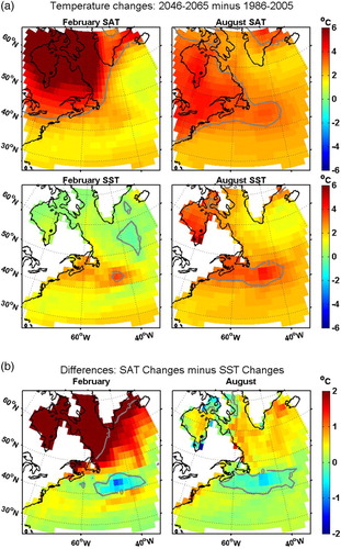
To examine the interrelation of these features further, the differences between the 60-year changes in SAT and the 60-year changes in SST were computed for each model (not shown) and for the ensemble-mean fields (shown in Fig. 19b for illustration). The SAT increases are larger than the SST increases in most parts of the open NWA in winter and summer, consistent with atmospheric warming being the primary driver of ocean warming (e.g., Collins et al., 2013; Hegerl et al., 2007). However, there is a mid-latitude zonal band extending from near the Scotian Shelf across the Newfoundland Basin to the central North Atlantic (and present in all of the ESMs to some degree, although at varying locations) in which the SST changes are larger than the SAT changes, approximately collocated with the enhanced SAT and SST change features. This suggests that changes in ocean circulation in the ESMs, and the northward expansion of the subtropical gyre in particular, are important factors to the projected enhanced SAT changes in the mid-latitude zonal band extending eastward from the Scotian Shelf. An examination of the corresponding 60-year climate changes in sea surface height (SSH) in two of the ESMs (CanESM2, GFDL-ESM2M) in Loder and van der Baaren (2013) confirmed SSH changes in this region consistent with a relaxation and northward expansion of the subtropical gyre.

It should be cautioned, however, that although the potential for a northward expansion of the NWA's subtropical gyre (and a northward shift of the Gulf Stream) is substantive (e.g., Saenko et al., 2005) with a potential influence on local SAT, it is unclear whether the enhanced mid-latitude SAT and SST changes in the present ESMs are reliable, in view of the latter's poor representation of the gyre–gyre boundary discussed earlier. This is an example of how deficiencies in the representation of ocean circulation and its variability in AOGCMs could contaminate projections of atmospheric changes. On the other hand, an additional atmospheric advective contribution from the enhanced SAT over the continent to the enhanced SAT and SST in its lee (especially where the SAT changes exceed those in SST) remains probable.

Somewhat similarly, the area of simulated past and future SST decreases to the south of Greenland in most of the ESMs (Fig. 8) reflects a change in ocean circulation that dominates atmospheric warming. This may have some realism (e.g., in contributing to the observed warming hole; Drijfhout et al., 2012), but it could also reflect an unreliable change in the gyre–gyre interaction and/or AMOC in the models.

8 Summary and discussion

We have examined the spatial and temporal variability of selected physical variables in the NWA in the historical and two RCP simulations of six CMIP5 ESMs. A set of observational comparisons and projected 60-year changes for four variables (SAT, SIC, SST, and SSS) using interpolated bidecadal monthly means from a six-member ensemble of Run 1 from the ESMs has been presented, and we also examinedvariability in SAT, SST, and SSS among five runs of CanESM2. Subsurface temperature and salinity, as well as OML-max were examined in five and four of the ESMs, respectively, and long-term variability in SAT, SST, and SSS was examined in two ESMs.

The climatological annual cycles of SAT (during 1986–2005) are approximately reproduced at most sites in most of the ESMs, but past decadal-scale regional variability (since 1950) is not. For SST and SSS, agreement between the model and observed annual cycles is reduced compared with that for SAT, particularly for SSS. The large-scale SST and SSS patterns of the NWA's subpolar and subtropical gyres are approximately reproduced in the models, but there are significant differences in the location and structure of the boundary between the gyres. In particular, the subtropical gyre is too far north to the west of the Grand Bank in the models and not far enough north to the east of Flemish Cap. Seasonal ice cover in most of the models does not extend as far equatorward along the coast as observed but extends too far south in the Labrador Sea and, probably related to the latter, the OML-max distributions indicate that there is much less deep convection in the Labrador Sea than observed (in three of the four models). Further, observed decadal-scale SST and SSS variability in the NWA is not reproduced by the ESMs which, as for SAT, is not unexpected considering their initialization and coarse resolution (Taylor et al., 2012).

Collectively, the comparisons indicate that there are substantial differences in the representation of coupled ice–ocean variability in the NWA among the models and in the detailed spatial and temporal patterns between the models and observations. It appears doubtful that any of the models have an adequate representation of regional ice–ocean dynamics to reliably simulate ocean climate variability and change in the NWA, but it is also unclear whether any single model examined is worse than any of the others to the point that it should be rejected from an ensemble approach to regional climate change projections. The observational annual-cycle comparisons for SAT, SST, and SSS at selected sites, indicating that the observed bidecadal monthly means are generally within the combined observational and inter-model SEs of the ensemble monthly means in the historical simulations, provide some encouragement for the utility of an ensemble approach to coarse-scale climate change projections from the ESMs. On the other hand, because the models do not have an adequate representation of some key dynamical and thermodynamical processes in the NWA, their structural as well as parametric uncertainties need to be recognized in using their projections even in an ensemble approach (e.g., Collins et al., 2013; Shepherd, 2014).

The projected ensemble-mean increases in SAT show the previously identified (e.g., Meehl et al., 2007) Arctic amplification in winter and the weaker mid-latitude continental amplification in summer, with both having mid-latitude extensions over the NWA. As a result, the winter SAT changes are larger at higher latitudes and smaller at mid-latitudes, and there is no clear seasonal variation at mid-latitudes. However, the inter-model spread of the projected changes is of comparable magnitude to the ensemble-mean changes (except for northern areas in winter), such that there is substantial uncertainty regarding the magnitude of the changes. The projected ensemble-mean 60-year changes in SIC show seasonal reductions in the areas of the NWA that are near the limit of seasonal ice cover in the historical simulations, consistent with expectations for atmospheric warming. It is noteworthy that, in the different models, the offshore extent of the winter area of amplified SAT increase approximates that of the winter offshore extent of sea ice in the Labrador Sea, suggesting an interrelation (e.g., excessive initial ice resulting in excessive future warming) that may have implications for the reliability of detailed projections of both SAT and SIC for the region (e.g., Bracegirdle & Stephenson, 2013).

The projected ensemble-mean SST changes over the NWA are largest in a mid-latitude zonal band of warming extending eastward from the Scotian Shelf and Grand Bank region, with largest magnitudes (>4°C for RCP8.5) and extent in summer. This feature bears some similarity to the zonal band of amplified SAT increases that extends offshore from the continent at mid-latitudes in summer, pointing to the likelihood of an interrelation between the SAT and SST changes. The larger magnitudes of the SST increases (compared with the SAT increases) in a zonal band in, and/or just south of, the Grand Bank region in both summer and winter (Fig. 19) indicate that the northward expansion of the subtropical gyre in the models is a major contributor to this feature. Considering the models’ poor representation of the gyre–gyre boundary, this raises questions about the reliability of the details of both the SAT and SST mid-latitude change features, which may have implications for other atmospheric changes in the region, such as the projected northward shift of storm tracks identified in an earlier version of CanESM2 (e.g., Jiang & Perrie, 2007).

In the NWA's northern areas, the ensemble-mean SST climate changes are smaller (than in mid-latitudes), except in the Baffin Bay and coastal regions in summer where there is notable warming. In winter, there is an area of cooling south of Greenland similar to that in previous model projections and usually attributed to a projected reduction in the AMOC (e.g., Meehl et al., 2007). This feature extends into the Labrador Sea in some of the ESMs, resulting in little (ensemble-mean) warming in its eastern part in winter and only weak warming in summer. There is also no winter (SST) warming in the parts of Baffin Bay that remain ice covered in winter in the model projections (because of the insulating effect brought about by the sea ice and the SST remaining below freezing), in stark contrast to the amplified warming of the overlying atmosphere. Quantitative estimates of the 60-year SST changes for various NWA shelf regions, considering the ESMs’ simulations for both RCP4.5 and RCP8.5 (Loder & van der Baaren, 2013), are in the range of 0°–4°C in winter and 0°–5°C in summer. The ranges are similar for off-shelf areas, except for some models that project (near-surface) cooling in the Labrador Sea and waters south of Greenland (particularly in winter) and some that project localized areas of greater warming near the boundary of the subpolar and subtropical gyres.

The projected ensemble-mean SSS changes indicate a general pattern of year-round freshening over most of the NWA, as expected in subpolar waters, and a slight increase in SSS in the subtropical waters that encroach at mid-latitudes, also as expected. The transition line (no change in SSS) varies from model to model and lies near 40°N in the ensemble-mean pattern. However, the spread in the magnitude of the changes in both the six-member ESM ensemble and the five-member CanESM2 ensemble generally exceeds the magnitude of the ensemble-mean change, and there are qualitative inconsistencies among the annual cycles from some of the models in some areas, such that the magnitudes and detailed spatial structure of the SSS changes remain uncertain.

The projected changes in the vertical distribution of annual-mean temperature and salinity on the sections indicate that the SST and SSS changes are representative of widely varying upper-layer depths in the various models and areas covered. The peak warming is below the surface in some areas and at the surface in others, whereas the largest changes in salinity are generally at or near the surface. Considering the differences among the models in temperature and salinity on these sections in the 1986–2005 historical periods (Loder & van der Baaren, 2013), it is difficult to interpret the vertical structure of the changes and to assess their reliability without a more detailed examination.

The differing patterns of OML-max among the models and the poor agreement of these patterns with the subpolar areas of observed deep convection, raise further questions about the reliability of the projected subsurface temperature and salinity changes in the NWA. Realistic representation of the Labrador Sea's deep convection area appears to be particularly challenging for coarse-resolution AOGCMs because of the multiple contributing atmosphere, ice, and ocean factors (e.g., de Jong et al., 2009), including ocean eddies (Saenko et al., 2014). Nevertheless, the projected climate changes in OML-max in the four ESMs examined point to reduced depths of deep convection in the subpolar areas where it occurs, consistent with expectations, but also smaller increases in MLD in the subtropical gyre.

In conclusion, it should be emphasized that the six ESMs examined here are only one subset of the CMIP5 AOGCMs examined in IPCC AR5, and the CMIP5 models are only one of a number of information sources that need to be considered in developing projections and assessing their reliability for use in impact assessments, planning, and decision-making. With the limited number of models and information sources considered here (and the limitations of, and differences among, the models), it is not possible to provide firm quantitative estimates of the projected changes or to quantify their uncertainty. However, it is clear from the discrepancies between the historical simulations and observations for a number of key variables in the NWA that the present generation of AOGCMs continue to have problems with resolving important features (e.g., Arctic outflows, sea ice, ocean convection zones, ocean gyre boundaries, decadal variability) of the region's coupled atmosphere–ice–ocean system. There are also indications that some of these inadequacies may be degrading the representation of regional atmospheric variability. Thus, caution is needed in the use of projected changes from these (and previous) AOGCMs for the NWA, whether in using their outputs directly for impact assessments and adaptation planning or indirectly through inputs to regional downscaling models.

Acknowledgements

We acknowledge the World Climate Research Programme's Working Group on Coupled Modelling, which is responsible for CMIP, and we thank the climate modelling groups (listed in Table 1 of this paper) for producing and making available their model output. For CMIP the US Department of Energy's Program for Climate Model Diagnosis and Intercomparison provides coordinating support and led development of software infrastructure in partnership with the Global Organization for Earth System Science Portals.

We also gratefully acknowledge the availability of observational data from DFO's AZMP and AZOMP, EC's AHCCD, the international Argo program, and other institutes and international organizations. Key contributions to the study were the availability of surface fields from the six ESMs interpolated to a common grid provided by Jim Christian of DFO's Institute of Ocean Science (IOS) and observational time series from DFO's AZMP provided by Roger Pettipas of DFO's Bedford Institute of Oceanography, to whom we are very grateful. We also thank Diane Lavoie of DFO's Maurice Lamontange Institute (MLI) and colleagues at EC's CCCma for sharing model fields, Zeliang Wang for providing the HadISST1 bidecadal fields, and the following for other inputs to the study and/or comments on our earlier report or this paper: David Brickman, Jim Christian, Brendan DeTracey, Guoqi Han, Diane Lavoie, Warren Lee, Bill Merryfield, Ingrid Peterson, Jean-Philippe Paquin, and Oleg Saenko, as well as three anonymous reviewers.

Disclosure statement

No potential conflict of interest was reported by the authors.

Additional information

Funding

The work presented here was partly funded by DFO's ACCASP and Climate Change Science Initiative.

Appendix

The 0 and 10 m February and August climatologies for ocean temperature and salinity developed by co-author I. Yashayaev were computed as part of a North Atlantic Climatology atlas for standard depths (0 to 500 m) for the 1946–2002 period. A multi-pass horizontal weighting scheme was used to estimate monthly, seasonal, and annual means on a 0.3° × 0.3° grid from all available in situ observations, after screening for outliers and biases. Data sources included the World Ocean Database (http://www.nodc.noaa.gov/OC5/WOD/pr_wod.html), the Oceanographic database of the International Council for the Exploration of the Sea (http://ocean.ices.dk/HydChem/), databases of the World Ocean Circulation Experiment (from its website and CD-ROM), and archives of DFO's BIO, the State Oceanographic Institute (Moscow), the Institute of Oceanology of the Russian Academy of Science, and other institutions and groups. Discrete (e.g., bottle) data within 5 m of each of the 0 and 10 m levels were used directly, and higher-resolution (e.g., conductivity-temperature-depth (CTD) profiler) data within 5 m of each level were vertically averaged before being used.

The first pass of horizontal weighting and interpolation used only nearby data (within the distance between the horizontal grid points), whereas subsequent passes used more distant data in order to fill gaps left after the first pass. Various weighting schemes were used in the different passes including inverse distance, spatial anisotropy, statistical closeness of measurements, and representativeness based on the number of points used in the previous pass. The 0 and 10 m climatologies were averaged to obtain the 0–10 m climatologies, and these were further smoothed using an inverse-distance weighting scheme in order to obtain spatial resolution similar to that in the interpolated ESM fields.

References

- Andrews, T., Gregory, J. M., Webb, M. J., & Taylor, K. E. (2012). Forcing, feedbacks and climate sensitivity in CMIP5 coupled atmosphere-ocean climate models. Geophysical Research Letters, 39, L09712. doi:10.1029/2012GL051607
- Arora, V. K., Scinocca, J. F., Boer, G. J., Christian, J. R., Denman, K. L., Flato, G. M., … Merryfield, W. J. (2011). Carbon emission limits required to satisfy future representative concentration pathways of greenhouse gases. Geophysical Research Letters, 38, L05805. doi:10.1029/2010GL046270
- Bindoff, N. L., Willebrand, J., Artale, V., Cazenave, A., Gregory, J., Gulev, S., … Unnikrishnan, A. (2007). Observations: Oceanic climate change and sea level. In S. Solomon, D. Qin, M. Manning, Z. Chen, M. Marquis, K. B. Averyt, … H. L. Miller (Eds.), Climate change 2007: The physical science basis. Contribution of Working Group I to the Fourth Assessment Report of the Intergovernmental Panel on Climate Change (pp. 385–432). Cambridge, UK: Cambridge University Press.
- de Boyer Montégut, C., Madec, G., Fischer, A. S., Lazar, A., & Iudicone, D. (2004). Mixed layer depth over the global ocean: An examination of profile data and a profile-based climatology. Journal of Geophysical Research, 109, C12003. doi:10.1029/2004JC002378
- Bracegirdle, T. J., & Stephenson, D. B. (2013). On the robustness of emergent constraints used in multimodel climate change projections of Arctic warming. Journal of Climate, 26, 669–678. doi:10.1175/JCLI-D-12–00537.1
- Brock, R. J., Kenchington, E., & Martinez-Arroyo, A. (Eds.) (2012). Scientific guidelines for designing resilient Marine Protected Area networks in a changing climate. Commission for Environmental Cooperation. Montreal, Canada. Retrieved from http://www3.cec.org/islandora/en/item/10820-scientific-guidelines-designing-resilient-marine-protected-area-networks-in-changing-en.pdf
- Bryan, F. O., Hecht, M. W., & Smith, R. D. (2007). Resolution convergence and stability studies with North Atlantic circulation models. Part I: The western boundary current system. Ocean Modelling, 16, 141–159. doi:10.1016/j.ocemod.2006.08.005
- Capotondi, A., Alexander, M. A., Bond, N. A., Curchitser, E. N., & Scott, J. D. (2012). Enhanced upper ocean stratification with climate change in the CMIP3 models. Journal of Geophysical Research, 117, C04031. doi:10.1029/2011JC007409
- Cavalieri, D. J., & Parkinson, C. L. (2012). Arctic sea ice variability and trends, 1979–2010. The Cryosphere, 6, 881–889. doi:10.5194/tc-6–881–2012
- Chen, X., & Tung, K.-K. (2014). Varying planetary heat sink led to global-warming slowdown and acceleration. Science, 345(6199), 897–903. doi:10.1126/science.1254937
- Cheng, W., Chiang, J. C. H., & Zhang, D. (2013). Atlantic Meridional Overturning Circulation (AMOC) in CMIP5 models: RCP and historical simulations. Journal of Climate, 26, 7187–7197. doi:10.1175/JCLI-D-12–00496.1
- Christian, J. R., & Foreman, M. G. G. (Eds.) (2013). Climate trends and projections for the Pacific Aquatic Basin. (Canadian Technical Report of Fisheries and Aquatic Sciences, 3032). Retrieved from http://www.dfo-mpo.gc.ca/Library/350212.pdf
- Colbourne, E., Holden, J., Craig, J., Senciall, D., Bailey, W., Stead, P., & Fitzpatrick, C. (2014). Physical oceanographic conditions on the Newfoundland and Labrador Shelf during 2013. (Fisheries and Oceans Canada, Canadian Science Advisory Secretariat, Research Document, 2014/094). Retrieved from http://www.dfo-mpo.gc.ca/csas-sccs/publications/resdocs-docrech/2014/2014_094-eng.pdf
- Collins, M., Knutti, R., Arblaster, J., Dufresne, J.-L., Fichefet, T., Friedlingstein, P., … Wehner, M. (2013). Long-term climate change: Projections, commitments and irreversibility. In T. F. Stocker, D. Qin, G.-K. Plattner, M. Tignor, S. K. Allen, J. Boschung, A. Nauels, Y. Xia, V. Bex, & P. M. Midgley (Eds.), Climate change 2013: The physical science basis. Contribution of Working Group I to the Fifth Assessment Report of the Intergovernmental Panel on Climate Change (pp. 1029–1136). Cambridge, UK: Cambridge University Press.
- Collins, W. J., Bellouin, N., Doutriaux-Boucher, M., Gedney, N., Halloran, P., Hinton, T., … Woodward, S. (2011). Development and evaluation of an Earth-system model – HadGEM2. Geoscientific Model Development, 4, 1051–1075. doi:10.5194/gmd-4-1051-2011
- Cooke, M. A., Demirov, E., & Zhu, J. (2014). A model study of the relationship between sea-ice variability and surface and intermediate water mass properties in the Labrador Sea. Atmosphere-Ocean, 52, 142–154. doi:10.1080/07055900.2013.877417
- Dewar, W. K. (2001). On ocean dynamics in midlatitude climate. Journal of Climate, 14, 4380–4397. doi: 10.1175/1520-0442(2001)014<4380:OODIMC>2.0.CO;2
- DFO. (2013). Risk-based assessment of climate change impacts and risks on the biological resources and infrastructure within Fisheries and Oceans Canada's mandate – Atlantic Large Aquatic Basin. (Fisheries and Oceans Canada, Canadian Science Advisory Secretariat Science Response, 2012/044). Retrieved from http://www.dfo-mpo.gc.ca/csas-sccs/Publications/ScR-RS/2012/2012_044-eng.html
- Diffenbaugh, N. S., & Giorgi, F. (2012). Climate change hotspots in the CMIP5 global climate model ensemble. Climatic Change, 114, 813–822. doi:10.1007/s10584-012-0570-x
- Drijfhout, S., van Oldenborgh, G. J., & Cimatoribus, A. (2012). Is a decline of AMOC causing the warming hole above the North Atlantic in observed and modeled warming patterns?. Journal of Climate, 25, 8373–8379. doi:10.1175/JCLI-D-12-00490.1
- Dufresne, J.-L., Foujols, M.-A., Denvil, S., Caubel, A., Marti, O., Aumont, O., … Vuichard, N. (2013). Climate change projections using the IPSL-CM5 Earth System Model: From CMIP3 to CMIP5. Climate Dynamics, 40(9–10), 2123–2165. doi:10.1007/s00382-012-1636-1
- Dunne, J. P., John, J. G., Adcroft, A. J., Griffies, S. M., Hallberg, R. W., Shevliakova, E., … Zadeh, N. (2012). GFDL's ESM2 global coupled climate–carbon Earth System Models. Part I: Physical formulation and baseline simulation characteristics. Journal of Climate, 25, 6646–6665. doi:10.1175/JCLI-D-11-00560
- Durack, P. J., & Wijffels, S. E. (2010). Fifty-year trends in global ocean salinities and their relationship to broad-scale warming. Journal of Climate, 23, 4342–4362. doi:10.1175/2010JCLI3377.1
- Durack, P. J., Wijffels, S. E., & Matear, R. J. (2012). Ocean salinities reveal strong global water cycle intensification during 1950 to 2000. Science, 336, 455–458. doi:10.1126/science.1212222
- Flato, G., Marotzke, J., Abiodun, B., Braconnot, P., Chou, S. C., Collins, W., … Rummukainen, M. (2013). Evaluation of climate models. In T. F. Stocker, D. Qin, G.-K. Plattner, M. Tignor, S. K. Allen, J. Boschung, … P. M. Midgley (Eds.), Climate change 2013: The physical science basis. Contribution of Working Group I to the Fifth Assessment Report of the Intergovernmental Panel on Climate Change (pp. 741–866). Cambridge, UK: Cambridge University Press.
- Giorgetta, M. A., Jungclaus, J., Reick, C. H., Legutke, S., Bader, J., Böttinger, M., … Stevens, B. (2013). Climate and carbon cycle changes from 1850 to 2100 in MPI-ESM simulations for the Coupled Model Intercomparison Project 5. Journal of Advances in Modeling Earth Systems, 5(3), 572–597. doi:10.1002/jame.20038
- Hebert, D., Pettipas, R., Brickman, D., & Dever, M. (2014) Meteorological, sea ice and physical oceanographic conditions on the Scotian Shelf and in the Gulf of Maine during 2013. (Fisheries and Oceans Canada, Canadian Science Advisory Secretariat Research Document, 2014/070). Retrieved from http://www.dfo-mpo.gc.ca/csas-sccs/publications/resdocs-docrech/2014/2014_070-eng.pdf
- Hegerl, G. C., Zwiers, F. W., Braconnot, P., Gillet, N. P., Luo, Y., Marengo, J. A., … Stott, P. A. (2007). Understanding and attributing climate change. In S. Solomon, D. Qin, M. Manning, Z. Chen, M. Marquis, K. B. Averyt, … H. L. Miller (Eds.), Climate change 2007: The physical science basis. Contribution of Working Group I to the Fourth Assessment Report of the Intergovernmental Panel on Climate Change (pp. 663–745). Cambridge, UK: Cambridge University Press.
- Hu, X., & Myers, P. G. (2014). Changes to the Canadian Arctic Archipelago sea ice and freshwater fluxes in the twenty-first century under the Intergovernmental Panel on Climate Change A1B climate scenario. Atmosphere-Ocean, 52(4), 331–350. doi:10.1080/07055900.2014.942592
- Hurrell, J. W., & Deser, C. (2010). North Atlantic climate variability: The role of the North Atlantic Oscillation. Journal of Marine Systems, 79, 231–244. doi:10.1016/j.jmarsys.2009.11.002
- IPCC. (2007). Climate change 2007: The physical science basis. Contribution of Working Group I to the Fourth Assessment Report of the Intergovernmental Panel on Climate Change. In S. Solomon, D. Qin, M. Manning, Z. Chen, M. Marquis, K. B. Averyt, … H. L. Miller (Eds.). Cambridge, UK: Cambridge University Press.
- IPCC. (2013). Climate change 2013: The physical science basis. Contribution of Working Group I to the Fifth Assessment Report of the Intergovernmental Panel on Climate Change. In T. F. Stocker, D. Qin, G.-K. Plattner, M. Tignor, S. K. Allen, J. Boschung, … P. M. Midgley (Eds.) (p. 1535). Cambridge, UK: Cambridge University Press.
- Ishizaki, Y., Shiogama, H., Emori, S., Yokohata, T., Nozawa, T., Ogura, T., … Takahashi, K. (2012). Temperature scaling pattern dependence on representative concentration pathway emission scenarios. Climatic Change, 112, 535–546. doi:10.1007/s10584-012-0430-8
- Jahn, A., & Holland, M. (2013). Implications of Arctic sea ice changes for North Atlantic deep convection and the meridional overturning circulation in CCSM4-CMIP5 simulations. Geophysical Research Letters, 40, 1206–1211. doi:10.1002/grl.50183
- Jiang, J., & Perrie, W. (2007). The impacts of climate change on autumn North Atlantic midlatitude cyclones. Journal of Climate, 20, 1174–1187. doi:10.1175/JCLI4058.1
- Joly, S., Senneville, S., Caya, D., & Saucier, F. J. (2011). Sensitivity of Hudson Bay sea ice and ocean climate to atmospheric temperature forcing. Climate Dynamics, 36, 1835–1849. doi:10.1007/s00382-009-0731-4
- Jones, G. S., Stott, P. A., & Christidis, N. (2013). Attribution of observed historical near surface temperature variations to anthropogenic and natural causes using CMIP5 simulations. Journal of Geophysical Research, 118, 4001–4024. doi:10.1002/jgrd.50239
- de Jong, M. F., Drijfhout, S. S., Hazeleger, W., van Aken, H. M., & Severijns, C. A. (2009). Simulations of hydrographic properties in the northwestern North Atlantic Ocean in coupled climate models. Journal of Climate, 22, 1767–1786. doi:10.1175/2008JCLI2448.1
- Jungclaus, J. H., Fischer, N., Haak, H., Lohmann, K., Marotzke, J., Matei, D., … von Storch, J. S. (2013). Characteristics of the ocean simulations in MPIOM, the ocean component of the MPI-Earth System Model. Journal of Advances in Modeling Earth Systems, 5, 422–446. doi:10.1002/jame.20023
- Knutti, R., Masson, D. and Gettelman, A. (2013). Climate model genealogy: Generation CMIP5 and how we got there. Geophysical Research Letters, 40, 1194–1199. doi:10.10002/grl.50526
- Knutti, R., & Sedláček, J. (2013). Robustness and uncertainties in the new CMIP5 climate model projections. Nature Climate Change, 3, 369–373. doi:10.1038/nclimate1716
- Lavoie, D., Lambert, N., ben Mustafa, S., & van der Baaren, A. (2013a). Projections of future physical and biogeochemical conditions in the Northwest Atlantic from CMIP5 Global Climate Models. (Canadian Technical Report of Hydrography and Oceanographic Sciences, 285). Retrieved from http://www.dfo-mpo.gc.ca/Library/349066.pdf
- Lavoie, D., Lambert, N., & van der Baaren, A. (2013b). Projections of future physical and biogeochemical conditions in Hudson and Baffin Bays CMIP5 Global Climate Models. (Canadian Technical Report of Hydrography and Oceanographic Sciences, 289). Retrieved from http://www.dfo-mpo.gc.ca/Library/349552.pdf
- Levitus, S., Antonov, J. I., Boyer, T. P., Baranova, O. K., Garcia, H. E., Locarnini, R. A., Zweng, M. M. (2012). World ocean heat content and thermosteric sea level change (0–2000 m), 1955–2010. Geophysical Research Letters, 39, L10603. doi:10.1029/2012GL051106
- Li, G., Zhang, X., Zwiers, F., & Wen, Q. H. (2012). Quantification of uncertainty in high-resolution temperature scenarios for North America. Journal of Climate, 25, 3373–3389. doi:10.1175/JCLI-D-11-00217.1
- Loder, J. W., & van der Baaren, A. (2013). Climate change projections for the Northwest Atlantic from six CMIP5 Earth System Models. (Canadian Technical Report Hydrography and Oceanographic Sciences, 286). Retrieved from http://www.dfo-mpo.gc.ca/library/349550.pdf
- Loder, J. W., Petrie, B., & Gawarkiewicz, G. (1998). The coastal ocean off northeastern North America: A large-scale view. In A. R. Robinson & K. H. Brink (Eds.), The sea, volume 1: The global coastal ocean-regional studies and synthesis (pp. 105–133). New York: John Wiley & Sons, Inc.
- Loder, J. W., & Wang, Z. (2015). Trends and variability of sea surface temperature in the Northwest Atlantic from three gridded historical datasets. Atmosphere-Ocean. doi:10.1080/07055900.2015.1071237
- Maher, N., Sen Gupta, A., & England, M. H. (2014). Drivers of decadal hiatus periods in the 20th and 21st centuries. Geophysical Research Letters, 41(16), 5978–5986. doi:10.1002/2014GL060527
- Markovic, M., de Elía, R., Frigon, A., & Matthews, H. D. (2013). A transition from CMIP3 to CMIP5 for climate information providers: The case of surface temperature over eastern North America. Climatic Change, 120, 197–210. doi 10.1007/s10584-013-0782-8 doi: 10.1007/s10584-013-0782-8
- Mearns, L. O., Sain, S., Leung, L. R., Bukovsky, M. S., McGinnis, S., Biner, S., … Sloan, L. (2013). Climate change projections of the North American Regional Climate Change Assessment Program (NARCCAP). Climatic Change, 120, 965–975. doi:10.1007/s1058401308
- Meehl, G. A., Stocker, T. F., Collins, W. D., Friedlingstein, P., Gaye, A. T., Gregory, J. M., … Zhao, Z.-C. (2007). Global climate projections. In S. Solomon, D. Qin, M. Manning, Z. Chen, M. Marquis, K. B. Averyt, M. Tignor, & H. L. Miller (Eds.), Climate change 2007: The physical science basis. Contribution of Working Group I to the Fourth Assessment Report of the Intergovernmental Panel on Climate Change (pp. 747–845). Cambridge, UK: Cambridge University Press.
- Moss, R. H., Edmonds, J. A., Hibbard, K. A., Manning, M. R., Rose, S. K., van Vuuren, D. P., … Wilbanks, T. J. (2010). The next generation of scenarios for climate change research and assessment. Nature, 463, 747–756. doi:10.1038/nature08823.
- Nakićenović, N., Alcamo, J., Davis, G., de Vries, B., Fenhann, J., Gaffin, S., … Dadi, Z. (2000). IPCC special report on emissions scenarios. Cambridge, UK: Cambridge University Press. Retrieved from http://www.grida.no/publications/other/ipcc_sr/
- van Oldenburgh, G. J., Drijfhout, S. S., van Ulden, A. P., Haarsma, R., Sterl, C., Severijns, A., … Dijkstra, H. A. (2009). Western Europe is warming much faster than expected. Climate of the Past, 5, 1–12. doi: 10.5194/cp-5-1-2009
- Palmer, M. D., Good, S. A., Haines, K., Rayner, N. A., & Stott, P. A. (2009). A new perspective on warming of the global oceans. Geophysical Research Letters, 36, L20709. doi:10.1029/2009GL039491
- Peters, G. P., Andrew, R. M., Boden, T., Canadell, J. G., Ciais, P., Le Quéré, C., … Wilson, C. (2013). The challenge to keep global warming below 2° C. Nature Climate Change, 3, 4–6. doi:10.1038/nclimate1783
- Peterson, I. K., & Pettipas, R. (2013). Trends in air temperature and sea ice in the Atlantic Large Aquatic Basin and adjoining areas. (Canadian Technical Report of Hydrography and Oceanographic Sciences, 290). Retrieved from http://www.dfo-mpo.gc.ca/Library/350061.pdf
- Petrie, B., Loder, J. W., Akenhead, S., & Lazier, J. (1992). Temperature and salinity variability on the eastern Newfoundland Shelf: The residual field. Atmosphere-Ocean, 30, 120–139. doi: 10.1080/07055900.1992.9649433
- Polyakov, I. V., Alexeev, V. A., Bhatt, U. S., Polyakov, E. I., & Zhang, X. (2010). North Atlantic warming: Patterns of long-term trend and multidecadal variability. Climate Dynamics, 34, 439–457. doi:10.1007/s00382-008-0522-3
- Rayner, N. A., Parker, D. E., Horton, E. B., Folland, C. K., Alexander, L. V. Rowell, D. P., … Kaplan, A. (2003). Global analyses of sea surface temperature, sea ice, and night marine air temperature since the late nineteenth century. Journal of Geophysical Research, 108(D14), 4407. doi:10.1029/2002JD002670
- Reid, P. C., & Valdés, L. (2011). ICES status report on climate change in the North Atlantic. ICES Cooperative Research Report No. 310.
- Rogelj, J., Meinshausen, M., & Knutti, R. (2012). Global warming under old and new scenarios using IPCC climate sensitivity range estimates. Nature Climate Change, 2, 248–253. doi:10.1038/nclimate1385
- Saenko, O. A., Dupont, F., Yang, D., Myers, P. G., Yashayaev, I. & Smith, G. C. (2014). Role of resolved and parameterized eddies in the Labrador Sea balance of heat and buoyancy. Journal of Physical Oceanography, 44, 3008–3032. doi:10.1175/JPO-D-14-0041.1
- Saenko, O. A., Fyfe, J. C. & England, M. H. (2005). On the response of the oceanic wind-driven circulation to atmospheric CO2 increase. Climate Dynamics, 25, 415–426. doi: 10.1007/s00382-005-0032-5
- Serreze, M. C., & Barry, R. G. (2011). Processes and impacts of Arctic amplification: A research synthesis. Global and Planetary Change, 77, 85–96. doi:10.1016/j.gloplacha.2011.03.004.
- Shepherd, T. G. (2014). Atmospheric circulation as a source of uncertainty in climate change projections. Nature Geoscience, 7, 703–708. doi:10.1038/ngeo2253
- Sillmann, J., Kharin, V. V., Zhang, X., Zwiers, F. W., & Bronaugh, D. (2013a). Climate extremes indices in the CMIP5 multimodel ensemble: Part 1. Model evaluation in the present climate. Journal of Geophysical Research Atmospheres, 118, 1716–1733. doi:10.1002/jgrd.50203
- Sillmann, J., Kharin, V. V., Zhang, X., Zwiers, F. W., & Bronaugh, D. (2013b). Climate extremes indices in the CMIP5 multimodel ensemble: Part 2. Future climate projections. Journal of Geophysical Research Atmospheres, 118, 2473–2493. doi:10.1002/jgrd.50188
- Sou, T., & Flato, G. (2009). Sea ice in the Canadian Arctic Archipelago: Modeling the past (1950–2004) and the future (2041–60). Journal of Climate, 22, 2181–2198. doi:10.1175/2008JCLI2335.1
- Steiner, N. S., Christian, J. R., Six, K. D., Yamamoto, A., & Yamamoto-Kawai, M. (2014). Future ocean acidification in the Canada Basin and surrounding Arctic Ocean from CMIP5 earth system models. Journal of Geophysical Research: Oceans, 119, 332–347.
- Stocker, T. F., Qin, D., Plattner, G.-K., Alexander, L. V., Allen, S. K., Bindoff, N. L., … Xie, X.-P. (2013). Technical summary. In T. F. Stocker, D. Qin, G.-K. Plattner, M. Tignor, S. K. Allen, J. Boschung, … P. M. Midgley (Eds.), Climate change 2013: The physical science basis. Contribution of Working Group I to the Fifth Assessment Report of the Intergovernmental Panel on Climate Change (pp. 33–115). Cambridge, UK: Cambridge University Press.
- Stroeve, J. C., Kattsov, V., Barrett, A., Serreze, M., Pavlova, T., Holland, M. & Meier, W. N. (2012). Trends in Arctic sea ice extent from CMIP5, CMIP3, and observations. Geophysical Research Letters, 39, L16502. doi:10.1029/2012GL052676.
- Talley, L. D. & Raymer, M. E. (1982). Eighteen degree water variability. Journal of Marine Research, 40, 757–775.
- Taylor, K. (2012). CMIP5 standard_output. Retrieved from http://cmip-pcmdi.llnl.gov/cmip5/docs/standard_output.pdf
- Taylor, K. E., Stouffer, R. J., & Meehl, G. A. (2012). An overview of CMIP5 and the experiment design. Bulletin of the American Meteorological Society, 93, 485–498. doi:10.1175/BAMS-D-11-00094.1
- Terray, L. (2012). Evidence for multiple drivers of North Atlantic multi-decadal climate variability. Geophysical Research Letters, 39, L19712. doi: 10.1029/2012GL053046
- Ting, M., Kushnir, Y., & Li, C. (2014). North Atlantic multidecadal SST oscillation: External forcing versus internal variability. Journal of Marine Systems, 133, 27–38. doi:10.1016/j.jmarsys.2013.07.006
- Tivy, A., Howell, S. E. L., Alt, B., McCourt, S., Chagnon, R., Crocker, G., … Yackel, J. J. (2011). Trends and variability in the Canadian Arctic based on the Canadian Ice Service Digital Archive, 1960–2008 and 1968–2008. Journal of Geophysical Research, 116, C03007. doi:10.1029/2009JC005855
- Umoh, J. U., & Thompson, K. R. (1994). Surface heat flux, horizontal advection, and the seasonal evolution of water temperature on the Scotian Shelf. Journal of Geophysical Research, 99, 20403–20416. doi:10.1029/94JC01620
- Våge, K., Pickart, R. S., Thierry, V., Reverdin, G., Lee, C. M., Petrie, B., … Ribergaard, M. H. (2009). Surprising return of deep convection to the subpolar North Atlantic Ocean in winter 2007–2008. Nature Geoscience, 2, 67–72. doi:10.1038/NGEO382
- Vincent, L. A., Wang, X. L., Milewska, E. K., Wan, H., Yang, F., & Swail, V. (2012). A second generation of homogenized Canadian monthly surface air temperature for climate trend analysis. Journal of Geophysical Research, 117, D18110. doi:10.1029/2012JD017859
- van Vuuren, D. P., Edmonds, J., Kainuma, M., Riahi, K., Thomson, A., Hibbard, K., … Rose, S. K. (2011). The representative concentration pathways: An overview. Climatic Change, 109, 5–31. doi:10.1007/s10584-011-0148-z
- Wang, M., & Overland, J. E. (2012). A sea ice free summer Arctic within 30 years – an update from CMIP5 models. Geophysical Research Letters, 39, L18501. doi:10.1029/2012GL052868
- Wang, Q., Myers, P. G., Hu, X., & Bush, A. B. G. (2012). Flow constraints on pathways through the Canadian Arctic Archipelago. Atmosphere-Ocean, 50, 373–385. doi:10.1080/07055900.2012.704348
- Watanabe, S., Hajima, T., Sudo, K., Nagashima, T., Takemura, T., Okajima, H., … Kawamiya, M. (2011). MIROC-ESM 2010: Model description and basic results of CMIP5–20c3 m experiments. Geoscientific Model Development Discussions, 4, 845–872. doi:10.5194/gmd-4-845-2011
- Wu, L., Cai, W., Zhang, L., Nakamura, H., Timmerman, A., Joyce, T., … Giese, B. (2012). Enhanced warming over the global subtropical western boundary currents. Nature Climate Change, 2, 161–166. doi:10.1038/nclimate1353
- Yashayaev, I. (2007). Hydrographic changes in the Labrador Sea, 1960–2005. Progress in Oceanography, 73, 242–276. doi: 10.1016/j.pocean.2007.04.015
- Yashayaev, I., Head, E. J., Azetsu-Scott, K., Wang, Z., Li, W. K. W., Greenan, B. J. W., … Punschon, S. (2014) Oceanographic and environmental conditions in the Labrador Sea during 2012. (Fisheries and Oceans Canada, Canadian Science Advisory Document Research Document, 2014/046). Retrieved from http://www.dfo-mpo.gc.ca/csas-sccs/Publications/ResDocs-DocRech/2014/2014_046-eng.html
- Yashayaev, I., & Loder, J. W. (2009). Enhanced production of Labrador Sea Water in 2008. Geophysical Research Letters, 36, L01606. doi:10.1029/2008GL036162
- Zhai, X., Johnson, H. L., & Marshall, D. P. (2014). A simple model of the response of the Atlantic to the North Atlantic Oscillation. Journal of Climate, 27, 4052–4069. doi:10.1175/JCLI-D-13-00330.1
- Zhang, R., & Vallis, G. K. (2007). The role of bottom vortex stretching on the path of the North Atlantic western boundary current and on the northern recirculation gyre. Journal of Physical Oceanography, 37(8), 2053–2080. doi:10.1175/JPO3102.1