Investigating the Effect of Oceanographic Conditions and Swimming Behaviours on the Movement of Particles in the Gulf of St. Lawrence Using an Individual-Based Numerical Model

ABSTRACT

In this study an individual-based numerical model with three-dimensional (3D) and time-dependent fields of circulation and hydrography is used to examine the effects of the physical environment and various biological behaviours on the distribution and movement of particles in the Gulf of St. Lawrence and adjacent waters. The 3D circulation and hydrographic fields are simulated by a numerical ocean circulation model. The model domain covers the St. Lawrence Estuary (SLE), the Gulf of St. Lawrence (GSL), the Scotian Shelf, the Gulf of Maine, and their adjacent waters. The basis of the individual-based model is a numerical scheme that tracks the movement of particles carried by ocean currents. Several swimming behaviours of marine animals are considered with efficient seaward migration in the GSL as the goal. Electronic tagging data for the American eel (Anguilla rostrata) are used as guidance in specifying the behaviours. It is demonstrated that particles that undergo an observed behaviour, known as selective tidal stream transport, are able to exit the SLE more efficiently than particles that are carried passively by the 3D ocean currents. Outside the SLE, particles that search for and swim towards higher salinity move further downstream than those that have a preference for deeper water or swim in random directions.

RÉSUMÉ

[Traduit par la rédaction] Pour cette étude, nous utilisons un modèle numérique fondé sur les individus et dont les champs tridimensionnels hydrographiques et de circulation varient en fonction du temps, afin d'examiner les effets de l'environnement physique et de divers comportements biologiques sur la répartition et le mouvement des particules dans le golfe du Saint-Laurent et dans les eaux adjacentes. Un modèle numérique de circulation océanique simule les champs tridimensionnels hydrographiques et de circulation. Le domaine du modèle couvre l'estuaire et le golfe du Saint-Laurent, le plateau néo-écossais, le golfe du Maine, et les eaux adjacentes. Le modèle individu-centré s'appuie sur un schème numérique qui suit le mouvement de particules, que transportent les courants océaniques. Nous examinons le comportement natatoire de plusieurs animaux marins et visons notamment l'efficacité de la migration vers la mer à partir du golf du Saint-Laurent. Les données de marquage électronique d'anguilles (Anguilla rostrata) aident à déterminer les comportements. Nous démontrons que les particules manifestant un comportement, connu sous le nom de transport sélectif par courant de marée, sont capables de sortir plus efficacement de l'estuaire que les particules passivement transportées dans toutes les directions par les courants marins. Hors de l'estuaire, les particules qui recherchent une salinité accrue et nagent vers ce but se déplacent davantage vers l'aval que celles qui préfèrent les eaux profondes ou qui nagent dans des directions aléatoires.

KEYWORDS:

• ocean circulation model
• particle tracking
• individual-based model
• marine animal migration
• American eel
• St. Lawrence Estuary
• Gulf of St. Lawrence

1 Introduction

The world's fish consumption has grown steadily over the last five decades, with the global annual fish consumption increasing from an average of 9.9 kg per capita in the 1960s to 19.2 kg per capita in 2012 (Food and Agriculture Organization of the United Nations, 2014). One consequence of this continuous growth in fish consumption has been the depletion of many wild fish stocks. For example, the estimated loss of more than 90% of the world's large oceanic fish occurred between the 1950s and l990s as a result of industrialized fisheries (Myers and Worm, 2003). In order to protect the remaining fish stocks, fishery management policies have to be formulated on the ecosystem scale, as indicated by the statistical study of Worm et al. (2006) who found that the viability of fisheries is correlated with the health of the ecosystem in which they reside. Management on the ecosystem scale, in turn, requires better understanding of the distribution and migration of marine animals.

In the last few decades, the development of various electronic tag technologies has greatly aided in the collection of information about the distribution and migration of marine animals (Cooke et al., 2011). One type of electronic tag is the acoustic tag, which transmits information about its identity (and possibly other types of data) received and recorded by hydrophones when the tag is within their detection range (generally <1 km). Another type is the archival tag, which stores data internally. The data can be collected when the archival tag is retrieved or transmitted to satellites when the tag is at the water surface (Nelson et al., 2013).

In parallel to the tracking of marine animals using electronic tags and other observational methods, such as the use of genetic analysis to determine the origin of individuals in seasonal aggregations (Wirgin et al., 2012), various statistical and numerical methods have been increasingly used to study the abundance and movement of marine animals on time scales of days to months. One such method is the state-space model, which can be used to identify the types of behaviours represented in the electronic tag records and to estimate the values of parameters for those behaviours (Jonsen, Mills Fleming, and Myers, 2005). Another approach is to simulate a marine animal population by mathematically formulating its biological processes, such as recruitment and vulnerability to fishing at a given age (Walters, Martell, and Korman, 2006). Traditionally, the output of population-scale numerical biological models has been the population-averaged values of variables. However, the increasing availability of computing resources in recent decades has given rise to the individual-based model, which simulates biological processes at the level of individuals or small groups of individuals in the population (Gentleman, 2002). The use of an individual-based model requires information about biological behaviours and physical environmental conditions that are specific to the species and geographical area to be studied. For example, Bonhommeau et al. (2009) included a behaviour known as diel vertical migration in a numerical particle-tracking model to examine the effect of this behaviour on the distribution of European eel (Anguilla anguilla) larvae as they are carried by ocean currents in the North Atlantic. The inclusion of diel vertical migration was motivated by the observational study of Castonguay and McCleave (1987), who collected vertically discrete water samples at different times of the day to observe diel vertical migration of eel larvae in the North Atlantic.

In our study, we combine an individual-based model of marine animal movement with three-dimensional (3D), time-varying fields of circulation and hydrography. The latter are produced by a numerical ocean circulation model. The main objective of our study is to investigate the effects of the physical environment and various biological behaviours on the spatial distribution of animals in the ocean at time scales of O(weeks) using the individual-based model. The basis of the individual-based model is a numerical particle-tracking scheme, in which the particles represent marine animals. In its basic application, particle-tracking schemes calculate the movement of passive particles carried by ocean currents. Passive particle-tracking has been used in many applications including trajectories of oil from a spill incident (e.g., Mariano et al., 2011) and planktons that cause shellfish poisoning (Trites and Drinkwater, 1991). In this study, the distribution of particles in the passive case is used as a baseline in the discussion of numerical experiments that include various observed and hypothesized biological behaviours. It will be shown that particles carried passively by the ocean currents tend to be trapped in the estuary where the particles are released, and it is necessary to include biological behaviours in the particle-tracking schemes in order for particles to effectively exit the estuary and move seaward. To the best of our knowledge, the current study is one of the first attempts (if not the first) to parameterize biological behaviours in an individual-based model for the nektonic maturing phase of a fish species by using electronic tag-based field observations of swimming behaviour undertaken by that species. It should be noted, however, that, as will be described in Section 2, there have been several past studies using individual-based models of planktonic species or the planktonic phase of fish species in the St. Lawrence Estuary (SLE)–Gulf of St. Lawrence (GSL) region in which the specified biological behaviours were inferred from observations.

The individual-based model is applied to the SLE and the GSL. We based the choice of this region on three factors: (i) this region is home to a rich ecosystem (including several commercial fisheries) and is also an economically active area with heavily used shipping lanes; (ii) a numerical ocean circulation model for the region has been developed and extensively validated (Ohashi, Sheng, Thompson, Hannah, and Ritchie, 2009; Ohashi and Sheng, 2013); and (iii) marine nektonic animals were tracked in this region using electronic tag technologies as part of an international research project (Cooke et al., 2011). The tag-based field observations are used here to parameterize biological behaviours undertaken by particles in the model.

We provide a brief description of the study region in the next section and describe the numerical circulation model in Section 3. We describe the individual-based model and the numerical experiments in Section 4 and describe the results of the experiments in Section 5. A discussion of the results and possibilities for future research are presented in Section 6.

2 Study region

The SLE–GSL system (Fig. 1) is one of the largest estuary-like bodies of water in the world by surface area (about 2 × 10⁵ km²). Its main source of fresh water is the St. Lawrence River (SLR), whose annual mean discharge at Québec is about 1.1 × 10³ m³ s⁻¹ (Bourgault and Koutitonsky, 1999). Just downstream of Québec, fresh water from the SLR meets the upstream reach of salt water at the head of the SLE. About 400 km downstream of Québec, the SLE widens abruptly and connects with the GSL. Exchanges between the GSL and the North Atlantic Ocean occur largely through Cabot Strait to the south of the GSL. Cabot Strait has a width of approximately 100 km and a maximum depth of approximately 480 m. A smaller amount of exchange also occurs through the Strait of Belle Isle at the northeast corner of the GSL. One of the major bathymetric features of the GSL is a trough known as the Laurentian Channel, which starts at the continental slope outside Cabot Strait and extends landward through the Strait into the GSL, with one channel shoaling in the SLE and two channels shoaling in the northeastern GSL. The southwest portion of the GSL, known as the Magdalen Shallows, has water depths that are generally less than 80 m (Koutitonsky and Bugden, 1991).

Fig. 1 The model domain and its major bathymetric features. Abbreviations are used for Rivière-du-Loup (RdL), the St. Lawrence Estuary (SLE), Strait of Belle Isle (SBI), Prince Edward Island (PEI), and the Bay of Fundy (BoF). Black lines with circles indicate idealized channels that represent rivers in the model. The initial release area of particles is outlined with a solid red line in the SLE. The dashed red line at the mouth of the SLE indicates the location at which STST ceases. Atlantic Zone Monitoring Program (AZMP) stations are indicated by numbers, and tide gauges are indicated by letters.

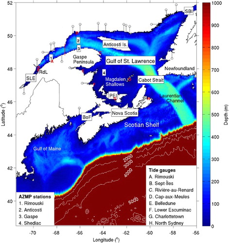
The main forcing for the circulation and hydrographic distributions over the SLE–GSL system includes the buoyancy forcing associated with river runoff, net heat and freshwater fluxes at the sea surface, wind stress, atmospheric pressure perturbations at sea level, tides, and oceanic input from the North Atlantic (Koutitonsky and Bugden, 1991). Freshwater discharge from the SLR is a major source of buoyancy forcing for the SLE–GSL system, which drives a buoyant estuarine plume with a surface-intensified outward (eastward) flow in the SLE. At the mouth of the SLE there is a southward flow from the north shore to the south shore that results in convergence of the SLE's outflow into the eastward-flowing Gaspé Current (Mertz, El-Sabh, and Koutitonsky, 1988). A portion of the Gaspé Current recirculates cyclonically within the northwest GSL and, together with westward flow along the north shore of the GSL, forms a cyclonic gyre known as the Anticosti Gyre (Sheng, 2001). The main branch of the Gaspé Current continues eastward along the Gaspé Peninsula and leaves the coast at the eastern tip of the Peninsula, carrying buoyant estuarine waters onto the Magdalen Shallows. The low-salinity estuarine waters exit the GSL through Cabot Strait (mainly on its western side). The above-mentioned buoyancy-driven surface circulation in the SLE and western GSL forms one limb of a cyclonic circulation pattern, which also consists of a northeastward flow along the Newfoundland coast and westward flow along the north shore of the GSL (Koutitonsky and Bugden, 1991). Variations in the atmospheric forcing, due to weather systems passing through the region, superimpose variations on the synoptic (O(days)) time scale over the general circulation pattern (Koutitonsky and Bugden, 1991).

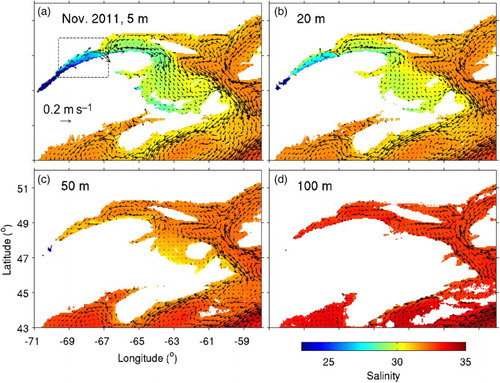
Figure 2 presents monthly-mean fields of salinity and currents in November 2011 at various depths in the SLE–GSL region and adjacent waters simulated by the ocean circulation model used in this study (more details are given in the next section). The 3D circulation model is able to reproduce the major features of the regional circulation discussed above, such as the Gaspé Current, the Anticosti Gyre, and the outflow from the GSL through the western side of Cabot Strait. The near-surface salinity fields (Figs 2a and 2b) have distinct spatial variations. The lowest salinity (<29) occurs in the SLE, and salinity in the northwest GSL and over the Magdalen Shallows is lower (<31) than in the northeastern part of the GSL (>31). The subsurface salinity fields (Figs 2c and 2d) are more homogeneous (about 32–34).

Fig. 2 Monthly-mean fields of salinity and currents for November 2011 calculated from model results at depths of (a) 5, (b) 20, (c) 50, and (d) 100 m in the St. Lawrence Estuary, Gulf of St. Lawrence, and eastern Scotian Shelf. Velocity vectors are shown at every fourth grid point. The dashed lines in (a) outline the area that will be shown in Fig. 3.

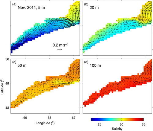
Figure 3 presents the simulated monthly-mean salinity and circulation fields within the SLE. The simulated circulation fields reproduce major observed circulation features of the SLE, such as the surface-intensified outward flow and the southward flow at the SLE mouth that results in the Gaspé Current. In the subsurface, there is flow towards the SLE head (especially along the north shore of the lower SLE), which is consistent with the circulation pattern that generally occurs in estuaries.

Fig. 3 Monthly-mean fields of salinity and currents for November 2011 calculated from model results at depths of (a) 5, (b) 20, (c) 50, and (d) 100 m in the St. Lawrence Estuary. Velocity vectors are shown at every model grid point.

Because of the significance of the SLE and GSL as fishery grounds, several studies have been made in the past to investigate the relationship between their physical and biological conditions. Statistical relationships were found between the discharge from the SLR and the abundance of commercially important fish species (Sutcliffe, 1973; Castonguay, Plourde, Robert, Runge, and Fortier, 2008). Interactions between physical conditions and life cycles of plankton species were studied using three-dimensional numerical circulation models coupled to ecosystem models (Zakardjian et al., 2003; Le Fouest, Zakardjian, and Saucier, 2005). The movement of the toxic dinoflagellate Alexandrium tamarense in this region has been studied by Trites and Drinkwater (1991) who treated them as passive, near-surface particles in a particle-tracking scheme and by Fauchot, Saucier, Levasseur, Roy, and Zakardjian (2008) in a coupled biological-physical model that demonstrated the role of wind-driven circulation in the development and movement of A. tamarense blooms in the lower SLE. Chassé and Miller (2010) identified important source and sink areas of American lobster (Homarus americanus) larvae in the GSL using an individual-based model, treating the larvae as passive particles that underwent settling to the bottom as a function of age and bottom temperature. Ouellet et al. (2013) applied Chassé and Miller's approach to capelin (Mallotus villosus) larvae in the SLE and GSL; particles representing larvae were inserted into the model at hatching locations determined from net surveys, and the model results provided new insights on the source regions of the larvae aggregations observed in various parts of the region. A behaviour known as diel vertical migration, whose effects on the migration of eels will be examined in this paper, has been included in several coupled biological-physical models of zooplanktons in this region (e.g., Sourisseau, Simard, and Saucier (2006), Maps, Zakardjian, Plourde, and Saucier (2011), Maps, Plourde, Lavoie, McQuinn, and Chassé (2014)).

The American eel (Anguilla rostrata) has traditionally been a commercially important species of fish in the SLE and GSL, as well as other coastal waters of North America. The spatial distribution of its larvae has suggested that the American eel spawns in the Sargasso Sea (Schmidt, 1925; McCleave, Kleckner, and Castonguay, 1987). The larvae, known as leptocephali, drift with ocean currents towards the east coast of North America (Fig. 4a). Within about a year of birth, they metamorphose into the juvenile stage, known as glass eel, and migrate into coastal and inland waters. They metamorphose through stages known as elvers and yellow eels, and after several years they metamorphose into a stage known as the silver eel as they migrate back to the Sargasso Sea for spawning (Tesch, 1977; Committee on the Status of Endangered Wildlife in Canada, 2012).

Fig. 4 (a) The life cycle of the American eel. Spawning takes place in the Sargasso Sea, and the larvae (leptocephali) are transported by ocean currents towards the east coast of North America. The juveniles (glass eels) migrate into coastal and inland waters and eventually metamorphose into yellow eels. During their seaward spawning migration, they metamorphose into silver eels. (Image reproduced by permission of the American Eel Monitoring Program at the Virginia Institute of Marine Science (http://www.vims.edu/research/departments/fisheries/programs/eel_survey/life_history/index.php). (b) Depth recorded every 15 minutes by an electronic tag attached to a silver American eel, released from Rivière-du-Loup in the SLE (Fig. 1). This dataset was also used in Fig. 2 of Béguer-Pon et al. (2012).

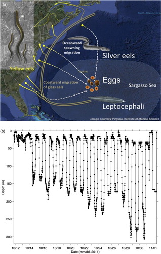
As part of an interdisciplinary research program known as the Ocean Tracking Network (OTN), American eels equipped with satellite archival tags or acoustic tags were released from the SLR and the SLE in an attempt to track their seaward migration to the Sargasso Sea (Béguer-Pon et al., 2012, 2014). The satellite archival tags (Béguer-Pon et al., 2012) recorded depth and temperature and indicated that the eels undertake a behaviour known as diel vertical migration (described in Section 4). These eels were lost to predation before they exited the GSL. Detection of acoustic tags (Béguer-Pon et al., 2014) strongly suggested that the eels undertake a behaviour known as selective tidal stream transport (described in Section 4) in the SLE, but no longer do so when they pass through Cabot Strait. In this study, information about the vertical movement of American eels from these tagging studies is used in the design of numerical experiments that include active swimming behaviour (described in Section 4).

3 The ocean circulation model

A brief description is given in this section of the numerical ocean circulation model that produces the 3D, time-varying fields of circulation and hydrography. These simulated 3D fields are subsequently used in various numerical experiments with the individual-based model (to be described in the next section). Passive particles are transported solely by the simulated circulation fields and by parameterized subgrid-scale processes. In the case of active particles, the particles also undertake various behaviours in response to the simulated 3D circulation and hydrography.

The regional ocean circulation model used in this study is based on the Princeton Ocean Model (POM; Mellor, 2004). The model set-up is similar to the one used by Ohashi and Sheng (2013), and the reader is referred to that paper for a more detailed discussion of the model set-up and validation. The model, as well as recent updates, is described briefly below.

The ocean circulation model uses a horizontal resolution of 1/16° in both the longitudinal and latitudinal directions. The model domain is 71.5°W–56°W and 38.5°N–52°N, which includes the GSL, the Scotian Shelf, the Bay of Fundy–Gulf of Maine system, and adjacent deep waters of the northwest Atlantic Ocean (Fig. 1). The model uses the terrain-following sigma vertical coordinate system, with 40 sigma layers. The model bathymetry was recently upgraded using the 30-arcsecond resolution General Bathymetric Chart of the Oceans (GEBCO; http://www.gebco.net). This was done by interpolating the GEBCO data onto the model's horizontal grid using one iteration of Barnes’ (1964) algorithm. The interpolated topographic data were smoothed using the algorithm of Martinho and Batteen (2006). The minimum water depth in the resulting model bathymetry is 10 m and the maximum water depth is approximately 5780 m. The model's horizontal eddy viscosity is calculated using the Smagorinsky scheme (i.e., the viscosity coefficient is a function of model grid size and horizontal current velocity gradients). It is recommended that the horizontal eddy diffusivity be kept small relative to the eddy viscosity (Mellor, 2004), so it is set to 1/10 of the viscosity (except in the southwest corner of the model domain, where it was found that setting the diffusivity equal to the viscosity was necessary in order to suppress spurious currents). The vertical mixing coefficients are calculated from the turbulence closure scheme suggested by Mellor and Yamada (1982).

To suppress systematic seasonal drift and bias in the model, the spectral nudging method (Thompson, Ohashi, Sheng, Bobanovic, and Ou, 2007) is used. This method includes frequency-dependent nudging terms in the tracer equations, which nudge the model temperature and salinity towards gridded climatologies of observed temperature and salinity at the mean, annual, and semi-annual time scales. Outside these time scales, the model's dynamics are not directly affected by the nudging and the model state variables evolve prognostically. In this study, spectral nudging is applied to the model temperature at all model grid cells and all depths. For the model salinity, the spectral nudging method is applied at all model grid cells at depths greater than 40 m, in order to prevent interference of the nudging method with the propagation of low-salinity waters from the SLE. In addition, the semi-prognostic method (Sheng, Greatbach, and Wright, 2001) is also used (at all model grid cells) to reduce drift in the simulated circulation. In this method, the simulated density in the hydrostatic equation is replaced by an average of that simulated density and the density calculated from climatological temperature and salinity. This is equivalent to adding a correction term to the horizontal momentum equations to prevent the simulated circulation from becoming unrealistic, while keeping the temperature and salinity equations prognostic.

At the sea surface, the ocean circulation model is forced by three-hourly atmospheric forcing including sea-level atmospheric pressure and wind stress. The atmospheric pressure was extracted from the North American Regional Reanalysis dataset (NARR; Mesinger et al., 2006). The wind stress was calculated from wind velocity in the NARR dataset (at 10 m above sea level) using the bulk formula of Large and Pond (1981). The ocean circulation model is also forced at the surface by the net heat flux, calculated from sea surface temperature (computed by the ocean circulation model) in combination with three-hourly NARR fields of air temperature, cloud cover, downward shortwave radiation flux, and precipitation (Mellor, 2004). The model does not include sea ice. As a result, the model does not simulate such physical processes as the contribution of sea-ice formation to the reduction in surface heat flux in winter or the contribution of sea-ice melt to the development of stratification in spring. The effect of salinity on the freezing point of water is also excluded by setting the minimum possible water temperature to −2°C regardless of the ambient salinity. We note, however, that using the spectral nudging method (described above) can account for these shortcomings to a certain extent, because the long-term averages of observed temperature and salinity (to which the simulated values are nudged) include the effects of sea-ice formation and melt.

Along lateral open boundaries of the ocean circulation model, the following three types of fields are specified: (i) hourly values of sea level and depth-mean currents produced by a barotropic version of the model covering the eastern Canadian seaboard, (ii) hourly values of tidal sea level and depth-mean currents, and (iii) daily values of 3D temperature, salinity, and currents simulated by a circulation model covering the northwest Atlantic (Urrego-Blanco and Sheng, 2012). The tidal forcing was recently upgraded to the “East coast of the USA” dataset of Oregon State University Tidal Prediction Software (OTPS; http://volkov.oce.orst.edu/tides/), which has a resolution of 1/30° (Egbert and Eroveeva, 2002). Rivers are represented by idealized channels cut into the model's coastline (Fig. 1). Daily values of river discharge are specified at the heads of these channels using the numerical scheme discussed by Ji, Sheng, Tang, Liu, and Yang (2011). For the SLR, the daily discharge values are obtained by temporal interpolation of monthly discharge estimates for the study period. For all other rivers, the daily discharge values are obtained by temporal interpolation of monthly climatological discharge observations. Details about the river discharge values and updates to them are described in Appendix A.

The ocean circulation model is initialized with monthly-mean climatological fields of temperature and salinity (unpublished data) processed using the methodology of Geshelin, Sheng, and Greatbach (1999). The ocean circulation model was started on 1 January 2010, and the 3D fields of currents and salinity were archived every hour between 15 September 2011 and 31 January 2012 to be used in this study.

Figure 5 shows scatterplots between the observed and simulated amplitudes and phases of tidal elevation for the M₂ and K₁ constituents at eight tide gauge locations (Fig. 1). Agreement between the observed and simulated values is quantified by γ², defined as the ratio of the hindcast error variance to the observed variance (Thompson and Sheng, 1997):(1)

Fig. 5 Scatterplots between observed and simulated amplitudes and phases of tidal elevations for the M₂ and K₁ tidal constituents for 2011 at the eight tide gauge locations shown in Fig. 1.

where Var stands for variance, and O and M denote, respectively, the observed and simulated values of a variable. Because γ² is dimensionless, its values for different variables (e.g., tidal elevations and salinity) can be compared directly as a way of evaluating model performance. For the eight tide gauge locations in the SLE and GSL, γ² is about 0.01 for both the amplitude and phase of both tidal constituents, which we consider to be very good agreement.

Figure 6 shows scatterplots between salinity values simulated by the circulation model for 2011 and their observed counterparts at Rimouski (in the SLE), Anticosti and Gaspé (both in the northwest GSL), and Shediac (over the Magdalen Shallows). The observations were made by the Atlantic Zone Monitoring Program (AZMP) managed by Fisheries and Oceans Canada (DFO). Agreement between the observed and simulated values of salinity is best in the SLE (Rimouski, where γ²= 0.08) and at the north shore of the northwest GSL (Anticosti, where γ²= 0.07), and deteriorates downstream with γ²= 0.34 at Shediac. Possible reasons for discrepancies between the simulated and observed salinity include the lack of sea ice in the circulation model and the use of climatological discharge values for rivers other than the SLR (Ohashi and Sheng, 2013). The other plausible reason for the high value of γ² at Shediac is the small number of observations available for comparison with model results (691 observations from nine cruises for Shediac compared with 3536 observations from 18 cruises for Rimouski).

Fig. 6 Scatterplots between simulated and observed salinity for 2011 at AZMP stations: (a) Rimouski, (b) Anticosti, (c) Gaspé, and (d) Shediac.

Comparisons between simulated and observed data for currents are not made in this study because of a lack of appropriate flow observations. It should be noted that Ohashi and Sheng (2013) compared simulated currents for the years 2000–2003 with observations from DFO's Ocean Data Inventory (Gregory, 2004) and demonstrated that the model performance is reasonable in simulating currents over the study region. The reader is referred to Ohashi and Sheng (2013) for a more detailed discussion of comparisons between the hydrography and circulation simulated by the circulation model and their observed counterparts.

4 The individual-based model

a Passive Movement

The passive movement of a particle can be described as the sum of movements due to currents and a “random walk” component:(2)

where and x^t are the 3D position vectors of a particle at times t+Δt and t, respectively, u(x, t) is the 3D vector of ambient currents, and δ is the 3D random walk component that represents movements associated with unresolved local processes (Shan, Sheng, and Greenan, 2014). In this study, the 3D movement of particles due to currents is calculated using the fourth-order Runge-Kutta method (Press, Teukolsky, Vetterling, and Flannery, 1992). The 3D components of δ, which are expressed as δ x, δ y, and δ z in the x, y, and z directions, respectively, can be expressed as (Taylor, 1922):(3)

where ξ _x, ξ _y, and ξ _z are random numbers in the range [−1,1] that have a Gaussian distribution centred on zero, and K_h and K_z are, respectively, the horizontal and vertical eddy diffusivity coefficients. It should be noted that the eddy diffusivity in Eq. (3) represents model-unresolved local processes such as small-scale circulation features associated with high-frequency winds. It differs from the eddy diffusivity used in the Reynolds-averaged temperature and salinity equations in the numerical ocean circulation model. The latter represents the contribution of subgrid-scale eddy processes to the Reynolds-averaged temperature and salinity fields.

The values of K_h and K_z estimated from field experiments have a large range; for example, Tseng (2002) estimated the horizontal diffusivity to range from 0.2 to 5 m² s⁻¹ in an estuary and around an island, and Riddle and Lewis (2000) found the vertical diffusivity estimated from experiments in various coastal and estuarine sites to range from 0.2 × 10⁻³ to about 10 × 10⁻³ m² s⁻¹. In this study, we follow Shan and Sheng (2012) and use values of diffusivity that lie in the middle of the orders of magnitude found in these studies, setting K_h to 1 m² s⁻¹ and K_z to 10⁻³ m² s⁻¹. Eddy diffusivity coefficients can vary in space and time; for example, Cyr, Bourgault, and Galbraith (2011) found that K_z at a location in the SLE ranges from O(10⁻⁵) m² s⁻¹ to O(10⁻³) m² s⁻¹ depending on the depth. A study of the sensitivity of particle movements to changes in the horizontal and vertical eddy diffusivity coefficients is presented in Section 4c1.

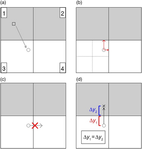
Calculation of a particle's movement defined in Eq. (2) does not consider the effect of local bathymetry. As a result of numerical errors in the particle-tracking scheme, it is possible that a particle is located within a wet grid cell of the circulation model at time t, but its predicted position is within a dry grid cell at time t+Δt. The following method is used to move such a particle back into a wet model grid cell (a schematic diagram of the method is shown in Fig. 7). If, for example, the predicted position of the particle is within the northeast quadrant of a dry grid cell of the model, the particle-tracking scheme searches for a wet grid cell among neighbouring cells to the north, east, and northeast. The order in which the neighbouring cells are checked depends on whether the particle is closer to the northern or eastern edge of the dry grid cell. If a wet grid cell is found among these neighbours, the particle is moved into that cell, and the particle's new position is such that its horizontal distance from the coast is the same as the distance by which it had moved inland from the coast before the correction. If none of the three neighbouring grid cells are located over water, the particle is moved back to its original position x^t. An alternative way to reduce the problem of particles moving into dry grid cells is to use simulated currents saved at shorter time intervals, but this approach was not pursued in our study.

Fig. 7 Schematic diagram for the manner in which the numerical particle-tracking scheme moves particles that have moved into a dry grid cell of the model back to a wet grid cell. The grey squares represent wet grid cells, and the white squares represent dry grid cells. (a) The particle is in cell 1 (a wet grid cell) at time t (at the position denoted by a square), but its calculated position for time t+Δt (denoted by a circle) is in cell 3 (a dry grid cell); (b) the particle-tracking scheme determines that the closest grid cell to the particle's provisional new position is cell 4, followed by cell 1; (c) however, the particle cannot move into cell 4 because it also is a dry grid cell; and (d) the particle moves northward into cell 1, and its new meridional distance from the coast (Δy₂) is of the same magnitude as the meridional distance by which it had moved inland in the provisional position (Δy₁).

b Particles with Biological Behaviour

The tracking scheme for passive particles discussed in the preceding section can be used to determine movements of inanimate particles such as marine debris or an oil slick. This scheme can also be used to track trajectories of fish larvae or small organisms that do not actively swim against currents. Some objects may undergo passive horizontal movements but maintain a constant vertical position because of buoyancy or vertical swimming, and the tracking scheme can be modified to simulate their movements. To track realistic movements of adult marine animals, however, it is necessary to include biological behaviours such as active swimming, feeding, and mortality. In this study, we focus solely on active swimming of marine animals.

To demonstrate the effect of specifying swimming behaviour in the movements of particles, this study uses example behaviours that have been observed or hypothesized for the American eel's seaward migration. The observed behaviours are those that were recorded by satellite archival tags and acoustic tags as the eels moved through the SLE and GSL (Béguer-Pon et al., 2012, 2014).

The behaviours observed in the American eel to be included in this study are diel vertical migration (DVM) and selective tidal stream transport (STST). These behaviours have also been observed in other species that inhabit the SLE and GSL; for example, the Greenland shark (Somniosus microcephalus) exhibits a daily cycle of depth preference in the SLE (Stokesbury, Harvey-Clark, Gallant, Block, and Myers, 2005), and the Atlantic mackerel (Scomber scombrus) appears to take advantage of the tidal cycle when entering the GSL through Cabot Strait (Castonguay and Gilbert, 1995). Thus, our model can be applied, with appropriate modifications, to other species.

1 Diel vertical migration

The definition of DVM is a biological behaviour in which a marine animal moves into deep waters at sunrise and moves towards the surface at sunset. This behaviour can be expressed as:(4)

where t+Δt is the time for which the particle's updated position is being calculated, t_rise is the time of sunrise, t_set is the time of sunset, is the particle's vertical position at time t+Δt, z_d is a depth near the bottom, and z_s is a depth near the surface. Both z_d and z_s are specified for each experiment (see Section 4c3). At times other than t_rise and t_set, the particle's updated vertical position is due to the vertical component of the random walk only (i.e., without vertical advection).

The proposed reasons for DVM include avoidance of visual predators (Iwasa, 1982) and, in the case of maturing European eel, regulation of body temperature in order to time their maturation to their arrival at spawning grounds (Aarestrup et al., 2009). It should be noted that some marine animals undergo reverse DVM, in which they ascend at dawn and descend at dusk, possibly to avoid predators (Ohman, Frost, and Cohen, 1983).

In this study, the ascent and descent in DVM are assumed to occur instantaneously at sunset and sunrise, respectively, based on the fact that vertical movements of silver American eels associated with DVM are mostly completed within one or two hours (Fig. 4b). Sunrise and sunset times at Rivière-du-Loup, Quebec (where the eels were released by Béguer-Pon et al. (2014)) were obtained from the website of the National Research Council of Canada (https://www.nrc-cnrc.gc.ca/eng/services/sunrise/advanced.html) and rounded to the nearest hour. The resulting sunrise and sunset times are shown in Table 1. Changes in sunrise and sunset times as particles move southward and eastward are relatively small. For example, during our study period (19 October to 18 December 2011), the maximum difference in sunrise times between Rivière-du-Loup and Sydney, Nova Scotia (on the western side of Cabot Strait) was 44 minutes, and the maximum difference in sunset times was 35 minutes. As a result, the latitudinal and longitudinal changes in sunrise and sunset times are ignored in this study.

Table 1. Sunrise and sunset times used in experiments that include DVM.

Dates	Sunrise	Sunset
19 October–6 November	1100 utc (0600 local time)	2200 utc (1700 local time)
7 November–1 December	1100 utc (0600 local time)	2100 utc (1600 local time)
2 December–3 February	1200 utc (0700 local time)	2100 utc (1600 local time)

2 Selective tidal stream transport

Another biological behaviour is STST in which a marine animal moves up the water column and moves laterally (either passively or swimming with the currents) when the tidal current is in a favourable direction and holds its position at the bottom during unfavourable tides. In the case of the American eel's seaward migration through an estuary, the eel moves to the bottom and ceases lateral movement during flood tide and moves up the water column and downstream during ebb tide (Parker and McCleave, 1997). (STST in the opposite direction with respect to tidal currents is undertaken, for example, by fish larvae that use STST to stay in estuaries (Rowe and Epifanio, 1994)). The acoustic telemetry observations of Béguer-Pon et al. (2014) strongly suggested that migrating silver American eels in the SLE undertake STST although the lack of depth measurements prevented the authors from making definite conclusions. The same study also found that the eels no longer undertake STST when they pass through Cabot Strait. Because it is not known where eels cease to undertake STST, in our numerical experiments the particles are programmed to carry out STST only within the SLE, with the mouth of the SLE defined at 67.3°W (Fig. 1).

To determine whether currents are in the flood or ebb phase in our experiments, they are first projected onto axes that are rotated 45° counter-clockwise (to approximately match the orientation of the SLE). If the zonal component of these currents (i.e., the component that is approximately parallel to the SLE) has a negative speed, the currents are considered to be in the flood phase; otherwise, the currents are considered to be in the ebb phase. A combination of STST with DVM is used to determine the vertical position of a particle as follows:(5)

where if u(x′, t) is the zonal component of the 3D, time-varying current simulated by the circulation model that has been projected onto the rotated grid, t_rise and t_set are the sunrise and sunset times of that day, and is the sunrise time of the following day. If the zonal component of the rotated current is negative (i.e., during flood tide), the particle moves to the bottom (z_d) regardless of the time of day. During ebb tide, the particle moves to z_d if it is daytime or to the surface (z_s) if it is night. The horizontal movement in experiments that include STST is defined as:(6a) (6b)

During flood tide, the particle stays at the bottom and does not undergo any horizontal movement. During ebb tide, the particle's new position is determined by physical processes (Eqs (2) and (3)), as well as any other biological behaviours (B_x and B_y) that are included in the numerical experiment.

3 swimming in horizontal directions

Although a marine animal can actively swim in three dimensions, in this study we only consider swimming behaviours in the horizontal directions because vertical swimming behaviour is at least partially accounted for by the DVM and STST. As examples of hypothesized behaviour, we formulate horizontal swimming behaviours that may guide the American eel as it swims across the GSL towards the open ocean. They are (i) swimming with a preference for deeper waters and (ii) swimming with a preference for higher-salinity waters (the latter having been suggested by the laboratory study of Hain (1975)). Numerical experiments using these three hypothesized swimming behaviours will be compared with a baseline case in which horizontal swimming is in random directions with the direction of swimming defined as:(7) where rand is a random number in the range [0,1]. Active swimming behaviours in the horizontal directions take place only outside the SLE (defined as the region to the east of 67.3°W).

c Description of Numerical Experiments

Particle movements in 19 numerical experiments are examined in our study (Table 2). In all the experiments, particles are released near Rivière-du-Loup, Quebec, from an area spanning 69.625°W to 69.500°W and 47.625°N to 48.375°N. The initial horizontal positions of the particles are 100 m apart. As a result, 11,921 particles are released in the area outlined in Fig. 1. Unless otherwise noted, all the particles are released at 1300 utc on 19 October 2011 at a depth of 20 m. The time and location of particle release were chosen to match those of the release of tagged silver American eels by Béguer-Pon et al. (2014). The numerical experiments are grouped as follows.

Table 2. List of the 19 numerical experiments conducted in this study. In experiments H1, H2, S1, S2, and W1, the lateral swimming speed is 0.5 m s⁻¹. The experiments are grouped as follows: Group A (experiments P1, P2, P3, P4, HM1, HP1, VM1, VP1, P1H, and P1D), Group B (experiments M1, M2, M3, and T1), and Group C (experiments H1, H2, S1, S2, and W1).

Experiment	Description
Group A
P1	Passive, released 20 m from surface, movement due to advection and subgrid-scale processes
P2	Similar to P1 but released 20 m above bottom or 90% of water depth if water depth <60 m
P3	Similar to P1 but with no vertical advection
P4	Similar to P2 but with no vertical advection
HM1	Similar to P1 but with horizontal eddy diffusivity set to 0.1 times the default value
HP1	Similar to P1 but with horizontal eddy diffusivity set to 10 times the default value
VM1	Similar to P1 but with vertical eddy diffusivity set to 0.1 times the default value
VP1	Similar to P1 but with vertical eddy diffusivity set to 10 times the default value
P1H	Similar to P1 but with release time of particles varied by up to 12 hours before and after default time, in one-hour increments
P1D	Similar to P1 but with release time of particles varied by up to 360 hours (15 days) before and after default time, in 24-hour increments
Group B
M1	Including DVM with upper limit (zs) set to 20 m below sea surface and lower limit (zd) set to 20 m above sea bottom or 90% of water depth if water depth <60 m. Particles cannot move below 300 m depth. Lateral movement is passive (similar to P3 and P4)
M2	Similar to M1 but with upper limit (zs) set to 5 m below the sea surface
M3	Similar to M1 but with lower limit (zd) set to 5 m above sea bottom for water depth >60 m
T1	Including DVM and STST with upper limit for both (zs) set to 20 m below sea surface and lower limit for both (zd) set to 20 m above sea bottom or 90% of water depth if water depth < 60 m. Lateral movement is passive
Group C
W1	Including DVM and STST as defined in T1 and, outside the SLE, lateral swimming in random directions generated every hour
H1	Including DVM and STST as defined in T1 and, outside the SLE, lateral swimming towards deeper water (up to 300 m depth) if found among surrounding model grid points. Search for deeper water occurs every hour during the day. If none is found or if it is night, lateral swimming in random direction generated every hour
H2	Similar to H1 but with search for deeper water occurring every other hour during the day
S1	Including DVM and STST as defined in T1 and, outside the SLE, lateral swimming towards higher salinity if found among surrounding model grid points. Search for higher salinity occurs every hour during the night. If none is found or if it is daytime, lateral swimming in random direction generated every hour
S2	Similar to S1 but with search for higher salinity occurring every four hours during the night

1 group a: particles with passive movement

Particles in the first group of experiments are purely passive and transported by the 3D currents. Particles are released at the 20 m depth in experiment P1 and near the bottom (20 m above the bottom for waters deeper than 60 m and 90% of the water depth for shallower waters) in experiment P2. Experiments P3 and P4 are similar to P1 and P2, respectively, except that the vertical movement of particles in P3 and P4 is due only to the vertical component of the random walk (i.e., there is no vertical advection).

To examine the effect of variations in the horizontal and vertical eddy diffusivities of the random walk component in experiments HM1 and HP1, the horizontal eddy diffusivity coefficient is decreased or increased by an order of magnitude, respectively, from the default value of 1 m² s⁻¹. In experiments VM1 and VP1, the vertical eddy diffusivity coefficient is decreased or increased by an order of magnitude, respectively, from the default value of 1 × 10⁻³ m² s⁻¹.

To examine the effect of temporal variations in the 3D circulation field on particle movement, two variations of experiment P1 are conducted. In experiment P1H, the release time is varied in 1–hour increments, up to 12 hours before or after the default release time. In experiment P1D, the release time of the particles is varied in 24-hour increments, up to 360 hours (15 days) before or after the default release time.

2 group b: the effect of diel vertical migration and selective tidal stream transport

In this group of experiments DVM and STST are added. The vertical movement of particles due to DVM is defined in Eq. (4). In experiment M1, the depth to which particles move at sunset (z_s in Eq. (4)) is set to 20 m, based on the typical near-surface position of the eels recorded in the archival tag data of Béguer-Pon et al. (2012; see our Fig. 4b). Because the horizontal coordinates of the eels as they migrated are not known, the lower limit of the eels’ vertical movement relative to the local water depth is not known. In this study, we set z_d (the depth to which a particle moves at sunrise) to 20 m above the bottom for local water depths deeper than 60 m and 90% of water depths for shallower waters. Particles cannot move below the 300 m depth, which is approximately the deepest vertical position recorded in the archival tag data of Béguer-Pon et al. (2012; see our Fig. 4b). In experiment M2, z_s is raised to 5 m, and in experiment M3, z_d for water depths greater than 60 m is lowered to 5 m above the bottom. The vertical movements are assumed to take place instantaneously. The horizontal movement of the particles is passive in both experiments.

In experiment T1 STST is added. The vertical movement of a particle due to STST and DVM is defined in Eq. (5). (No lower limits for vertical movements are defined for STST because this behaviour only takes place within the SLE where the maximum water depth is about 300 m.) Within the SLE, where STST is in effect, horizontal movement occurs as defined in Eq. (6). Outside the SLE, STST ceases but DVM continues to take place as defined in Eq. (4), and the horizontal movement of the particles is passive.

3 group c: the effect of active swimming in horizontal directions

In the remaining experiments, active swimming in horizontal directions is specified for particles outside the SLE (east of 67.3°W), so that the displacement of particles in these experiments is due to a combination of physical processes (as in the previous experiments) and swimming. The swimming speed is set to be constant at 0.5 m s⁻¹. This speed is equivalent to 0.5 body lengths (BL) per second for an average-length silver American eel starting its seaward migration from the SLE and corresponds to the shortest travel time of the four silver eels observed at Cabot Strait (out of 98 released in the SLE) by Béguer-Pon et al. (2014). Silver European eels are, however, estimated to travel at an average speed of about 0.5 BL s⁻¹ during their spawning migration, and in laboratory experiments they have been able to swim continuously at this speed for three months (van den Thillart et al., 2004) and at speeds as high as about 2 BL s⁻¹ continuously for at least several hours (Burgerhout et al., 2013). We therefore believe 0.5 m s⁻¹ to be a reasonable swimming speed in our experiments. In these experiments, STST (within the SLE only) and DVM are the same as in experiment T1.

In experiment W1, the horizontal swimming is in random directions. At each hour and for each particle, a random swimming direction is generated as defined in Eq. (7). Particles in experiments H1 and H2 include a preference for deeper waters. In experiment H1, each hour during the day (i.e., when the particle is in deep water because of DVM), the particle searches among the eight neighbouring model grid points for one with deeper water than the current model grid point. Model grid points with water depths greater than 300 m are ignored in the search. The particle swims in the direction of the neighbouring model grid point with the deepest water. If no neighbouring model grid points with deeper water are found, the particle swims in a random direction. Experiment H2 is similar to H1, but the search for deeper water takes place every other hour during the day. In both experiments the particle swims in random directions during the night, as in experiment W1.

Experiments S1 and S2 are similar to experiments H1 and H2, respectively, except that the search in S1 and S2 is for higher salinity instead of deeper water, and the search takes place during the night when the particle is near the surface where the salinity has a more pronounced horizontal structure (Fig. 3). The nighttime search for higher salinity takes place every hour in S1 and every four hours in S2. (The search interval for S2 was chosen so that a clear difference could be seen between the results of S1 and S2.) The particle swims in random directions during the day in both S1 and S2.

4 quantitative comparison of the numerical experiments

Differences in particle distributions among the numerical experiments described above are quantified in terms of the horizontal “centre of mass” of particles, which is defined as the average longitudinal and latitudinal coordinates of all particles. The experiments are compared in terms of the position of the centre of mass relative to the release location of the particles, as well as the mean and standard deviation of the particles’ distance from the centre of mass (rounded to the nearest kilometre) 60 days after the release of the particles. The results of different experiments are also compared in terms of the mean and standard deviation of the particles’ vertical positions (rounded to the nearest metre) after 60 days.

5 Results

a The Effects of Initial Depth and Vertical Advection, Diffusivity Coefficients, and Release Times (Group A)

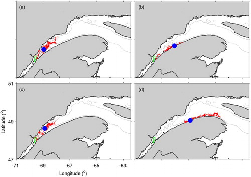
Figure 8 presents distributions of particles after 60 days in experiments P1 to P4. As mentioned above, in experiments P1 (Fig. 8a) and P2 (Fig. 8b) the movement of particles is purely passive, and the difference between the experiments is the initial vertical positions of the particles (near the surface in P1 and near the bottom in P2). The distribution of particles and the position of their centre of mass after 60 days are similar between the two experiments, with particles spanning the width of the SLE, some particles moving upstream from the release area, and a band of particles stretching from the mouth of the SLE along the north shore of the Gaspé Peninsula. The positions of the particles’ centre of mass are also similar between the two experiments.

Fig. 8 Distributions of particles after 60 days in (a) experiment P1 (passive particles released at 20 m depth), (b) experiment P2 (passive particles released near the bottom), (c) experiment P3 (similar to P1 but with no vertical advection), (d) experiment P4 (similar to P2 but with no vertical advection). The blue circle indicates the location of the centre of mass of the particles, and the area outlined in green represents the release area for the particles.

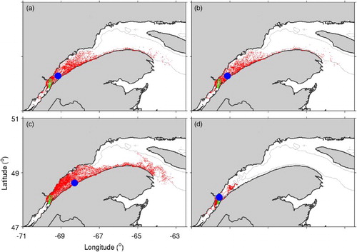
The similarity in particle distribution between experiments P1 and P2, despite the difference in circulation patterns between the near-surface and deeper waters (Figs 2 and 3), suggests that vertical advection plays an important role by moving particles away from their initial vertical positions and entraining them in different circulation patterns at different depths and the averaging of this effect over the more than 10,000 particles results in similar distributions despite the different initial depths of the particles. This is corroborated by experiments P3 and P4, which are similar to experiments P1 and P2, respectively, except that vertical advection is eliminated, such that the only vertical movement is due to the vertical component of the random walk. The distribution of particles in these experiments (Figs 8c and 8d) are very different, with the particle distribution in experiment P3 (released near the surface) being similar to those in P1 and P2 but with fewer particles upstream from the release area, more particles along the Gaspé Peninsula, and the centre of mass further downstream than in P1 and P2. This result reflects the outward flow near the surface in an estuarine circulation pattern (Fig. 3). In experiment P4 the particles are concentrated near the release area, reflecting the inward or weakly outward flow that exists in the subsurface of an estuary. Thus, the existence or lack of vertical advection plays an important role in the passive horizontal movement of particles on the time scale of O(weeks) in the SLE.

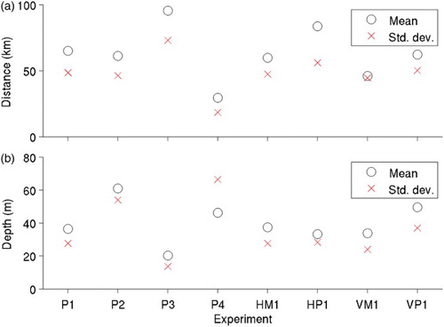
Figure 9 presents means and standard deviations of horizontal distances of particles from their centres of mass (Fig. 9a) and the particles' depths (Fig. 9b) at 60 days after release in experiments P1 to P4. The differences in the particles’ depths between experiments P1 and P3 and between P2 and P4 again indicate the important role played by vertical advection. Figure 9 also presents variations in distributions of particles when the horizontal and vertical eddy diffusivities of the random walk component (K_h and K_z, respectively) are increased or decreased by an order of magnitude from the default values used in experiment P1. The means and standard deviations of the particles’ horizontal distances from their centres of mass (Fig. 9a) are similar to that of experiment P1 when K_h is decreased in experiment HM1 or when K_z is increased in experiment VP1 (60 ± 47 km for HM1 and 62 ± 50 km for VP1 compared with 65 ± 49 km for P1). Increasing K_h (experiment HP1) or decreasing K_z (experiment VM1) results in larger differences from P1 (84 ± 56 km for HP1 and 46 ± 45 km for VM1). Increasing or decreasing K_h and decreasing K_z results in depth distributions (Fig. 9b) that are similar to that for experiment P1 (about 35 ± 25 m), but increasing K_z moves the particles deeper (50 ± 37 m). As discussed in Section 4a, the choice of an appropriate diffusivity value is difficult, and results of these experiments indicate that varying the diffusivity among possible values can have a large effect on the passive movement of particles.

Fig. 9 Means (circles) and standard deviations (crosses) for (a) horizontal distances of particles relative to the centre of mass and (b) depths of particles after 60 days, in experiments P1 to P4 and the experiments in group B (in which the horizontal eddy diffusivity of the random walk component is decreased (HM1) or increased (HP1) by an order of magnitude, or the vertical eddy diffusivity is decreased (VM1) or increased (VH1) by an order of magnitude.)

Figure 10 presents characteristics of particle distributions after 60 days in experiments P1H and P1D in terms of different particle release times. In experiment P1H, in which the particle release times are varied in one-hour increments, up to 12 hours before and after the default release time, differences in horizontal distances of particles from their centres of mass (Fig. 10a) and the particles' depths (Fig. 10b) appear to have semi-diurnal cycles, suggesting the influence of the semi-diurnal M₂ tidal constituent on the particles’ movements. The means and standard deviations of the distances of the particles from their centres of mass vary between 60 ± 49 km (when particles are released 12 hours before the default release time) and 78 ± 52 km (when particles are released six hours after the default release time). These two release times also result in the maximum (39 ± 27 m) and minimum (33 ± 30 m) particle depths, respectively.

Fig. 10 Means (circles) and standard deviations (crosses) for (a) horizontal distances of particles relative to the centre of mass and (b) depths of particles, in experiment P1H (passive particles with release times varied in one-hour increments, up to 12 hours, before and after the release time used in experiment P1); (c) and (d) are similar to (a) and (b) but for experiment P1D (similar to experiment P1H but with particle release times varied in one-day increments, up to 15 days, before and after the release time used in experiment P1).

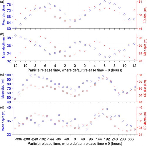
In experiment P1D (Figs 10c and Figs 10d), the particle release time is varied in one-day increments, up to 360 hours (15 days) before and after the default release time. The distances of the particles from their centres of mass vary in a way that suggests the influence of the spring-neap cycle, but the lack of a clear cycle suggests that the influence of the synoptic-scale (time scale of O(days)) variability in the circulation (due mainly to changes in atmospheric forcing) is also strong. The distances of the particles from their centres of mass reach a minimum value of 46 ± 44 km when particles are released 15 days before the default time and a maximum value of 99 ± 63 km when particles are released 10 days before the default time. The particles’ depths do not have a clear cycle, and their range is similar to that in experiment P1H, varying between 33 ± 29 m (when particles are released three days after the default time) and 39 ± 34 m (when particles are released eight days after the default time).

The results of experiments in this group indicate that the movement of particles on time scales of days to weeks can vary significantly depending on the existence or lack of vertical advection, the choice of eddy diffusivity coefficients, and changes in the circulation field resulting from the tidal cycle and atmospheric input. Despite these variations, in all of the experiments in this group, a large portion of the particles remained in the SLE after 60 days, which points to the necessity of particles employing active behaviour in order to efficiently move out of the SLE.

b The Effect of Diel Vertical Migration and Selective Tidal Stream Transport (Group B)

Figure 11 shows distributions of particles after 60 days from experiments M1 to M3, in which the particles undertake DVM and from experiment T1 in which they also undertake STST. The results of experiments M1 to M3 (Figs 11a–11c) reflect the fact that particles move twice a day between the near-surface and deeper waters but do not undergo vertical advection otherwise; the horizontal distribution can be seen as a combination of the downstream movement that occurred in experiment P3 and the horizontal concentration of particles that occurred in experiment P4. The larger concentration of particles along the south shore in experiment M2 reflects the horizontal shear in the near-surface currents simulated by our circulation model (Fig. 3a) in which currents are weaker along the south shore of the SLE. The distances of the particles from their centres of mass are 48 ± 21 km, 17 ± 18 km, and 25 ± 23 km, respectively, for experiments M1, M2, and M3, comparable to the distance of 29 ± 18 km for experiment P4.

Fig. 11 Distributions of particles after 60 days in (a) experiment M1 (the upper limit of DVM is the 20 m depth and the lower limit is 20 m above the bottom or 90% of the water depth if the water depth < 60 m); (b) experiment M2 (the upper limit of DVM is changed to the 5 m depth); (c) experiment M3 (the lower limit of DVM is changed to 5 m above the bottom if the water depth is > 60 m); and (d) experiment T1 (DVM is the same as in experiment M1, but STST is added). The blue circle indicates the location of the centre of mass of the particles and the area outlined in green represents the release area of particles.

Regardless of the changes in the upper and lower limits of the DVM among experiments M1 to M3, particles are still in the SLE after 60 days in these experiments. Although it is not exactly known why silver American eels undertake DVM (as discussed in Section 4b), the results of these experiments strongly suggest that DVM does not contribute to an efficient migration out of the SLE (unless the phases of DVM and STST happen to match favourably with ebb tides during the near-surface phase of DVM and flood tides during the bottom phase).

Figure 11d shows the distribution of particles from experiment T1, in which particles undertake DVM as in experiment M1 but also undertake STST. In this case, all the particles have exited the SLE after 60 days. This indicates that STST is a useful strategy for marine animals trying to exit an estuary, allowing them to take advantage of the seaward phase of strong tidal flows. The position of the particles’ centres of mass, however, indicates that many particles are still located near the mouth of the SLE after 60 days. The spread of particles about the centre of mass is again relatively low (40 ± 34 km).

c The Effect of Active Swimming in Horizontal Directions (Group C)

The previous group of experiments showed that although DVM does not contribute to migration out of the SLE, STST is an efficient strategy for moving out of the SLE. In this section, we examine the effect of adding different horizontal swimming behaviours once the particles have moved out of the SLE. We compare two behaviours, swimming with a preference for deeper water (experiments H1 and H2) and with a preference for higher salinity (experiments S1 and S2), to a baseline case in which particles swim in random directions (experiment W1). Although the focus of this study is the fall (when the American eel starts its seaward migration) and the experiments have focused on a 60-day period from October to December, for experiment W1 the distribution of particles after 120 days will also be shown in order to illustrate the tendency of particle movement in the GSL over a longer time scale.

In experiments H1, H2, S1, and S2, distributions of particles are sensitive to the frequency at which the particles check their surrounding conditions. In experiment H1 (Fig. 12a), in which particles look for deeper water every hour during the day (when they are in deeper water due to DVM), the particles are concentrated in a narrow band and their centre of mass is near the mouth of the SLE. In terms of moving downstream, this case is even less efficient than experiment W1 (Fig. 12e), in which particles swim in random directions. In experiment H2 (Fig. 12b), in wich particles look for deeper water every other hour during the day, the particles are still concentrated in a band, but their centre of mass is now at about the same location as in experiment W1. These results suggest that, although searching for deeper water may seem to be an efficient strategy for marine animals to orient themselves towards the open ocean, performing the search too frequently will cause to the particles to become “trapped” in local features. (It should also be noted that, in an estuarine circulation system, subsurface currents tend to be towards the head or weakly seaward).

Fig. 12 Distributions of particles after 60 days in (a) experiment H1 (when outside the SLE, particles search for surrounding model grid points with deeper water every hour during the day and swim towards it if one is found; otherwise, they swim in random directions); (b) experiment H2 (similar to H1 but searching for deeper water every other hour during the day); (c) experiment S1 (when outside the SLE, particles search for surrounding model grid points with higher salinity every hour during the night and swim towards it if one is found; otherwise, they swim in random directions); (d) experiment S2 (similar to S1 but searching for higher salinity every four hours during the night); and (e) experiment W1 (particles swim in random directions during all hours when outside the SLE). (f) Distribution of particles after 120 days in experiment W1.

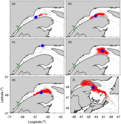
In experiment S1 (Fig. 12c), in which particles look for higher salinity every hour during the night (when they are in shallower water), after 60 days the particles are concentrated on the north shore of the GSL, where the salinity tends to be higher (Fig. 2). In experiment S2 (Fig. 12d) the centre of mass is slightly more downstream than in the other experiments. Thus, as was the case for deeper water, swimming with a preference for higher salinity becomes more efficient when the search for higher salinity is performed less frequently. These results suggest that, if marine animals are to migrate seaward by orienting themselves with respect to their surroundings, they need to use a strategy to detect large-scale gradients and ignore small-scale changes.

When experiment W1 is run for 120 days (Fig. 12f), particles tend to travel along the edge of the Magdalen Shallows and leave through the western side of Cabot Strait, consistent with the prevailing circulation pattern (Fig. 2). However, many particles are trapped in the northwest GSL, where a cyclonic gyre exists. This again suggests that marine animals migrating seaward from the SLE and GSL need to employ effective orientation and swimming strategies in order to reach the open ocean in a timely manner.

6 Discussion and conclusions

In this study we used an individual-based model with 3D currents and hydrography to examine the effects of physical oceanographic conditions and various swimming behaviours on the movements and distributions of particles in the SLE and the GSL at time scales of O(weeks). The time-varying, 3D fields of currents and hydrography were simulated by a numerical ocean circulation model. Electronic tag observations of the movements of the American eel in the SLE and GSL were used as a guide in formulating the swimming behaviours. The basis of the individual-based model used in this study is a numerical particle-tracking scheme that calculates movement of particles carried by ocean currents. In experiments in which the particle movements were purely passive, most of the particles tended to stay inside the SLE for several weeks or longer. More particles escaped from the SLE if they were released near the surface and did not undergo vertical advection, but even in this case, a large portion of the particles remained in the SLE even after 60 days. This suggests that other strategies, such as STST and active swimming behaviours, must be undertaken by marine animals, such as the American eel, in order to exit quickly from the SLE. Experiments in which the release time of particles was varied suggest that both the release times and temporal and spatial variations of the circulation field can influence the movements and distributions of passive particles in the study region.

Several types of swimming behaviours were formulated and added to the passive movement of particles. The swimming behaviour known as DVM was recorded by archival tags attached to eels, and STST behaviour was strongly suggested by acoustic telemetry observations of the eels’ lateral movements. The addition of DVM resulted in movement of the particles through the SLE that was even less efficient than in the passive cases, which suggests that migrating American eels must have a strong motivation to undertake this behaviour despite its negative effect on migration efficiency. This is consistent with the results of past studies in which simulation of zooplankton populations in the SLE–GSL region using coupled biological-physical models suggested that, although DVM likely evolved in these species to balance the need to be near the surface (to feed) and in deeper waters (to avoid predators), this behaviour can also help these populations from being flushed out of the region. For example, Maps et al. (2011) suggested that DVM is one of the crucial factors that maintain the population of the copepod Calanus finmarchicus in the SLE–GSL region, while Sourisseau et al. (2006) and Maps et al. (2014) suggested, respectively, that the lengths of time spent near the surface and near the bottom in DVM and the vertical extents of DVM have a significant effect on the lateral transport of krill populations in the region. By comparison, the addition of STST resulted in all the particles leaving the SLE within 60 days, which suggests that STST is an important swimming strategy for marine animals, such as American eels, to migrate from estuarine waters to the open ocean.

Our study also examined several other hypothesized biological behaviours that may help orient the eels seaward. These hypothesized behaviours took effect once the particles left the SLE. Among these behaviours, searching for and swimming towards higher salinity every four hours when near the surface was the most efficient in terms of moving the particles downstream. However, all the particles in the experiments in our study were within or just outside the SLE after 60 days, whereas the tagging study of Béguer-Pon et al. (2014) found that silver American eels released at the same location as the particles in our study were able to reach Cabot Strait between 18.5 and 39.4 days after release. This suggests that silver American eels employ very efficient swimming strategies for orienting themselves and swimming through the SLE and across the GSL. Possibilities for these strategies include active STST (in which eels anchoring themselves at the sea bottom detect the direction of ambient currents during favourable tide phases and swim in that direction) and the use of geomagnetic orientation (which has been suggested by the laboratory study of Durif et al. (2013)).

In summary, four major scientific findings have been made in this study based on analyses of particle movements produced by the individual-based model in 19 experiments. (i) Active swimming behaviour plays a very important role for silver American eels to efficiently exit the SLE. (ii) STST is a useful strategy for the eels to exit the SLE. (iii) By comparison, DVM is not a useful strategy for the eels to exit the SLE; therefore, this behaviour must be motivated by other reasons. (iv) Orientation with respect to water depth or salinity is not a very efficient strategy; therefore, eels probably employ other strategies to orient themselves as they swim across the GSL.

This study can be expanded to include (i) temporal variation in the behaviours (e.g., ceasing STST according to ambient salinity), (ii) a combination of several behaviours, and (iii) tests of additional behaviours (e.g., active STST or geomagnetic orientation) and parameters (e.g., variations in swimming speed), in order to identify the behaviours and parameters that can best reproduce the observed movements and migrations of the American eel and other marine animals.

Acknowledgements

We thank Mélanie Béguer-Pon, Julian Dodson (Laval University), and Martin Castonguay (DFO) for sharing observational data of the movement of American eels in the SLE–GSL and information about past studies on anguillid species. Numerical simulations using the circulation model were made on clusters maintained by the Atlantic Computational Excellence Network (ACENet). NARR data are made publicly available by the Physical Sciences Division, Earth System Research Laboratory, (U.S.) National Oceanic and Atmospheric Administration (http://esrl.noaa.gov/psd/data/narr/). Observations from tide gauges and the AZMP are made publicly available by DFO (http://www.meds-sdmm.dfo-mpo.gc.ca/isdm-gdsi/index-eng.html). Comments from two anonymous reviewers led to significant improvements in the manuscript. We also benefited from discussions with Keith Thompson and Shiliang Shan.

Disclosure statement

No potential conflict of interest was reported by the authors.

Additional information

Funding

This work is a contribution to OTN Canada, funded by the National Science and Engineering Research Council of Canada. Jinyu Sheng is supported by the Lloyd's Register Foundation, which helps protect life and property by supporting engineering-related education, public engagement, and the application of research.

Appendix A. Specification of freshwater discharge from rivers in the model

Freshwater discharge from rivers is specified in the ocean circulation model using the methodology described in Ohashi and Sheng (2013). Major upgrading of freshwater discharge in the model was made recently for major rivers in the GSL and adjacent waters. Freshwater discharge from the SLR is taken from estimates of monthly-mean discharge at Québec calculated by the Canadian Hydrographic Service using the regression model of Bourgault and Koutitonsky (1999) and obtained from the St. Lawrence Global Observatory (http://slgo.ca/en/runoffs/data/tables.html). Monthly-mean discharges of remaining rivers in the study region were obtained from the Water Survey of Canada (http://wateroffice.ec.gc.ca/search/search_e.html?sType=h2oArc) and averaged over all years with complete records. Table A1 lists rivers that have recently been added to our circulation model or those whose mean discharges have been recalculated with updated data, along with the stations and years used.

Table A1. List of major rivers in the St. Lawrence Estuary and Gulf of St. Lawrence, station names, and years of observation periods.

Status in the model	River name	Station name	Year(s) of observations used
Updated Rivers	St. Lawrence	Québec	2011
	Moisie	02UC002	1966–2012 excluding 1967, 1999, 2000, 2002, and 2006
	Romaine	02VC001	1957–2012 excluding 1960, 2002, and 2007
	Petit Mécatina	02XA008	1995 and 1998–2012 excluding 2005–2006
	Saint-Paul	02XC001	1968–2012 excluding 1972, 1981, 1990, 1996–1999, 2002, and 2005–2006
	Restigouche	01BJ007	1969–2012
New Rivers	Saguenay	02RH019	1943–1993
	Betsiamites	02SB004	1964–1994 excluding 1990
	Outardes	02TE001	1923–1977 excluding 1929–1931
	Manicouagan	02TC001	1947–1979
	Matane	02QB001	1927–2012 excluding1940
	Nabisipi	02WA001	1963–1987
	Aguanus	02WA002	1963–1981
	Humber	02YL003	1983–2013

References

- Aarestrup, K., Okland, F., Hansen, M. M., Righton, D., Gargan, P., Castonguay, M., … McKinley, R. S. (2009). Oceanic spawning migration of the European eel (Anguilla anguilla). Science, 325, 1660. doi: 10.1126/science.1178120
- Barnes, S. L. (1964). A technique for maximizing details in numerical weather map analysis. Journal of Applied Meteorology, 3, 396–409. doi:http://dx.doi.org/10.1175/1520-0450(1964)003<0396:ATFMDI>2.0.CO;2
- Béguer-Pon, M., Benchetrit, J., Castonguay, M., Aarestrup, K., Campana, S. E., Stokesbury, M. J., & Dodson, J. J. (2012). Shark predation on migrating adult American eels (Anguilla rostrata) in the Gulf of St. Lawrence. PLoS ONE, 7(10), e46830, 1–11. doi:10.1371/journal.pone.0046830
- Béguer-Pon, M., Castonguay, M., Benchetrit, J., Hatin, D., Legault, M., Verreault, G., … Dodson, J. (2014). Large scale migration patterns of silver American eels (Anguilla rostrata) from the St. Lawrence River to the Gulf using acoustic telemetry. Canadian Journal of Fisheries and Aquatic Sciences, 71, 1579–1592. doi:10.1139/cjfas-2013-0217
- Bonhommeau, S., Le Pape, O., Gascuel, D., Blanke, B., Tréguier, A.-M., Grima, N., … Rivot, E. (2009). Estimates of the mortality and the duration of the trans-Atlantic migration of European eel Anguilla anguilla leptocephali using a particle tracking model. Journal of Fish Biology, 74, 1891–1914. doi:10.1111/j.1095–8649.2009.02298.x
- Bourgault, D., & Koutitonsky, V. G. (1999). Real-time monitoring of the freshwater discharge at the head of the St. Lawrence Estuary. Atmosphere-Ocean, 37, 203–220. doi: 10.1080/07055900.1999.9649626
- Burgerhout, E., Tudorache, C., Brittijn, S. A., Palstra, A. P., Dirks, R. P., & van den Thillart, G. E. E. J. M. (2013). Schooling reduces energy consumption in swimming male European eels, Anguilla anguilla L. Journal of Experimental Marine Biology and Ecology, 448, 66–71. doi: 10.1016/j.jembe.2013.05.015
- Castonguay, M., & Gilbert, D. (1995). Effects of tidal streams on migrating Atlantic mackerel, Scomber scombrus L. ICES Journal of Marine Science, 52, 941–954. doi: 10.1006/jmsc.1995.0090
- Castonguay, M., & McCleave, J. D. (1987). Vertical distributions, diel and ontogenic vertical migrations and net avoidance of leptocephali of Anguilla and other common species in the Sargasso Sea. Journal of Plankton Research, 9, 195–214. doi: 10.1093/plankt/9.1.195
- Castonguay, M., Plourde, S., Robert, D., Runge, J. A., & Fortier, L. (2008). Copepod production drives recruitment in a marine fish. Canadian Journal of Fisheries and Aquatic Sciences, 65, 1528–1531. doi: 10.1139/F08-126
- Chassé, J. & Miller, R. (2010). Lobster larval transport in the southern Gulf of St. Lawrence. Fisheries Oceanography, 19, 319–338. doi:10.1111/j.1365-2419.2010.00548.x
- Committee on the Status of Endangered Wildlife in Canada. (2012). COSEWIC assessment and status report on the American Eel Anguilla rostrata in Canada. Ottawa: Committee on the Status of Endangered Wildlife in Canada.
- Cooke, S. J., Iverson, S. J., Stokesbury, M. J., Hinch, S. G., Fisk, A. G., VanderZwaag, D. L., … Whoriskey, F. (2011). Ocean tracking network Canada: A network approach to addressing critical issues in fisheries and resource management with implications for ocean governance. Fisheries, 36, 583–592. doi: 10.1080/03632415.2011.633464
- Cyr, F., Bourgault, D., & Galbraith, P. S. (2011). Interior versus boundary mixing of a cold intermediate layer. Journal of Geophysical Research, 116, C12029, 1–12. doi:10.1029/2011JC007359
- Durif, C. M. F., Browman, H. I., Phillips, J. B., Skiftesvik, A. B., Vøllestad, L. A., & Stockhausen, H. H. (2013). Magnetic compass orientation in the European eel. PLoS ONE, 8, e59212, 1–7. doi:10.1371/journal.pone.0059212
- Egbert, G. D., & Eroveeva, S. Y. (2002). Efficient inverse modeling of barotropic ocean tides. Journal of Atmospheric and Oceanic Technology, 19, 183–204. doi:10.1175/1520-0426(2002)019
- Fauchot, J., Saucier, F. J., Levasseur, M., Roy, S., & Zakardjian, B. (2008). Wind-driven river plume dynamics and toxic Alexandrium tamarense blooms in the St. Lawrence estuary (Canada): A modeling study. Harmful Algae, 7, 214–227. doi:10/1016/j.hal.2007.08.002
- Food and Agriculture Organization of the United Nations. (2014). The state of world fisheries and aquaculture 2014. Rome: Food and Agriculture Organization of the United Nations.
- Gentleman, W. (2002). A chronology of plankton dynamics in silico: How computer models have been used to study marine ecosystems. Hydrobiologia, 480, 69–85. doi: 10.1023/A:1021289119442
- Geshelin, Y., Sheng, J., & Greatbatch, R. J. (1999). Monthly mean climatologies of temperature and salinity in the western North Atlantic (Canadian Technical Report of Hydrography and Ocean Sciences 153). Dartmouth: Bedford Institute of Oceanography.
- Gregory, D. N. (2004). Ocean Data Inventory (ODI): A database of ocean current, temperature and salinity time series for the northwest Atlantic (Canadian Science Advisory Secretariat Research Document 2004/097). Dartmouth: Bedford Institute of Oceanography.
- Hain, J. H. W. (1975). The behaviour of migratory eels, Anguilla rostrata, in response to current, salinity, and lunar period. Helgoländer wissenschaftliche Meerersuntersuchungen, 27, 211–233. doi: 10.1007/BF01611808
- Iwasa, Y. (1982). Vertical migration of zooplankton: A game between predator and prey. The American Naturalist, 120, 171–180. doi: 10.1086/283980
- Ji, X., Sheng, J., Tang, L., Liu, D., & Yang, X. (2011). Process study of circulation in the pearl river estuary and adjacent coastal waters in the wet season using a triply-nested circulation model. Ocean Modelling, 38, 138–160. doi:10.1016/j.ocemod.2011.02.010
- Jonsen, I. D., Mills Fleming, J., & Myers, R. A. (2005). Robust state-space modeling of animal movement data. Ecology, 86, 2874–2880. doi: 10.1890/04-1852
- Koutitonsky, V. G., & Bugden, G. L. (1991). The physical oceanography of the Gulf of St. Lawrence: A review with emphasis on the synoptic variability of the motion. In J.-C. Therriault (Ed.), The Gulf of St. Lawrence: Small ocean or big estuary? ( Canadian Special Publication of Fisheries and Aquatic Sciences 113, pp. 57–90). Ottawa, Ontario: Fisheries and Oceans Canada.
- Large, W. G., & Pond, S. (1981). Open ocean momentum flux measurements in moderate to strong winds. Journal of Physical Oceanography, 11, 324–336. doi: 10.1175/1520-0485(1981)011<0324:OOMFMI>2.0.CO;2
- Le Fouest, V., Zakardjian, B., & Saucier, F. J. (2005). Seasonal versus synoptic variability in planktonic production in a high-latitude marginal sea: The Gulf of St. Lawrence (Canada). Journal of Geophysical Research, 110, C09012, 1–21. doi:10.1029/2004JC002423
- Maps, F., Plourde, S., Lavoie, D., McQuinn, I., & Chassé, J. (2014). Modelling the influence of daytime distribution on the transport of two sympatric krill species (Thysanoessa raschii and Meganyctiphanes norvegica) in the Gulf of St. Lawrence, eastern Canada. ICES Journal of Marine Science, 71, 282–292. doi:10.1093/icesjms/fst021
- Maps, F., Zakardjin, B. A., Plourde, S., & Saucier, F. J. (2011). Modeling the interactions between the seasonal and diel migration behaviours of Calanus finmarchicus and the circulation in the Gulf of St. Lawrence (Canada). Journal of Marine Systems, 88, 183–202. doi:10.1016/j.jmarsys.2011.04.004
- Mariano, A. J., Kourafalou, V. H., Srinivasan, A., Kang, H., Halliwell, G. R., Ryan, E. H., & Roffer, M. (2011). On the modeling of the 2010 Gulf of Mexico oil spill. Dynamics of Atmospheres and Oceans, 52, 322–340. doi:10.1016/j.dynatmocd.2011.06.001
- Martinho, A. S., & Batteen, M. L. (2006). On reducing the slope parameter in terrain-following numerical ocean models. Ocean Modelling, 13, 166–175. doi:10.1016/j.ocemod.2006.01.003
- McCleave, J. D., Kleckner, R. C., & Castonguay, M. (1987). Reproductive sympatry of American and European eels and implications for migration and taxonomy. American Fisheries Symposium, 1, 286–297.
- Mellor, G. L. (2004). Users guide for a three-dimensional, primitive equation, numerical ocean model. Princeton, NJ: Princeton University.
- Mellor, G. L. & Yamada, T. (1982). Development of a turbulence closure model for geophysical fluid problems. Reviews of Geophysics and Space Physics, 20, 851–875. doi: 10.1029/RG020i004p00851
- Mertz, G., El-Sabh, M. I., & Koutitonsky, V. G. (1988). Wind-driven motions at the mouth of the Lower St. Lawrence Estuary. Atmosphere-Ocean, 26, 509–523. doi: 10.1080/07055900.1988.9649315
- Mesinger, F., DiMego, G., Kalnay, E., Mitchell, K., Schaffran, P. C., Ebisuzaki, W., … Shi, W. (2006). North American regional reanalysis. Bulletin of the American Meteorological Society, 87, 343–360. doi:10.1175/BAMS-87-3-343
- Myers, R. A., & Worm, B. (2003). Rapid worldwide depletion of predatory fish communities. Nature, 423, 280–283. doi:10.1038/nature01610
- Nelson, T. C., Doukakis, P., Lindley, S. T., Schreier, A. D., Hightower, J. E., Hildebrand, L. R., … Webb, M. A. H. (2013). Research tools to investigate movements, migrations, and life history of sturgeons (Acipensderidae), with an emphasis on marine-oriented populations. PLoS ONE, 8(8), e71552, 1–22. doi:10.1371/journal.pone.0071552
- Ohashi, K., & Sheng, J. (2013). Influence of the St. Lawrence river discharge on the circulation and hydrography in Canadian Atlantic waters. Continental Shelf Research, 58, 32–49. doi:10.1016/j.csr.2013.03.005
- Ohashi, K., Sheng, J., Thompson, K. R., Hannah, C. G., & Ritchie, H. (2009). Numerical study of three-dimensional shelf circulation on the Scotian shelf using a shelf circulation model. Continental Shelf Research, 29, 2138–2156. doi:10.1016/j.csr.2009.08.005
- Ohman, M. D., Frost, B. W., & Cohen, E. B. (1983). Reverse diel vertical migration: An escape from invertebrate predators. Science, 220, 1404–1407. doi: 10.1126/science.220.4604.1404
- Ouellet, P., Bui, A. O. V., Lavoie, D., Chassé, J., Lambert, N., Ménard, N., & Sirois, P. (2013). Seasonal distribution, abundance, and growth of larval capelin (Mallotus villosus) and the role of the Lower Estuary (Gulf of St. Lawrence, Canada) as a nursery area. Canadian Journal of Fisheries and Aquatic Sciences, 70, 1508–1530. doi: 10.1139/cjfas-2013-0227
- Parker, S. J., & McCleave, J. D. (1997). Selective tidal stream transport by American eels during homing movements and estuarine migration. Journal of the Marine Biological Association of the United Kingdom, 77, 871–889. doi: 10.1017/S0025315400036237
- Press, W. H., Teukolsky, S. A., Vetterling, W. T., & Flannery, B. P. (1992). Numerical recipes in FORTRAN (2nd ed.). Cambridge: Cambridge University Press.
- Riddle, A. M. & Lewis, R. E. (2000). Dispersion experiments in U.K. coastal waters. Estuarine, Coastal, and Shelf Science, 51, 243–254. doi:10.1006/ecss.2000.0661
- Rowe, P. M., & Epifanio, C. E. (1994). Tidal stream transport of weakfish larvae in Delaware Bay, USA. Marine Ecology Progress Series, 110, 105–114. doi: 10.3354/meps110105
- Schmidt, J. (1925). The breeding places of the eel. In Annual report of the board of regents of the Smithsonian institution, 1924 (pp. 279–316). Washington, DC: Government Printing Office.
- Shan, S. & Sheng, J. (2012). Examination of circulation, flushing time and dispersion in Halifax Harbour of Nova Scotia. Water Quality Research Journal of Canada, 47, 353–374. doi:10.2166/wqrjc.2012.041
- Shan, S., Sheng, J., & Greenan, B. J. W. (2014). Modelling study of three-dimensional circulation and particle movement over the Sable Gully of Nova Scotia. Ocean Dynamics, 64, 117–142. doi:10.1007/s10236-013-0672-7
- Sheng, J. (2001). Dynamics of a buoyancy-driven coastal jet: The Gaspé Current. Journal of Physical Oceanography, 31, 3146–3162. doi: 10.1175/1520-0485(2001)031<3146:DOABDC>2.0.CO;2
- Sheng, J., Greatbatch, R. J., & Wright, D. G. (2001). Improving the utility of ocean circulation models through adjustment of the momentum balance. Journal of Geophysical Research, 106, 16711–16728. doi: 10.1029/2000JC000680
- Sourisseau, M., Simard, Y., & Saucier, F. J. (2006). Krill aggregation in the St. Lawrence system, and supply of krill to the whale feeding grounds in the estuary from the gulf. Marine Ecology Progress Series, 314, 257–270. doi: 10.3354/meps314257
- Stokesbury, M .J. W., Harvey-Clark, C., Gallant, J., Block, B. A., & Myers, R. A. (2005). Movement and environmental preferences of Greenland sharks (Somniosus microcephalus) electronically tagged in the St. Lawrence Estuary, Canada. Marine Biololgy, 148, 159–165. doi:10.1007/s00227-005-0061-y
- Sutcliffe, W. H. Jr. (1973). Correlations between seasonal river discharge and local landings of American lobster (Homarus americanus) and Atlantic halibut (Hippoglossus hippoglossus) in the Gulf of St. Lawrence. Journal of the Fisheries Research Board of Canada, 30, 856–859. doi:10.1139/f73-146
- Taylor, G. I. (1922). Diffusion by continuous movements. Proceedings of the London Mathematical Society, s2-20, 196–212. doi:10.1112/plms/s2-20.1.196
- Tesch, F.-W. (1977). The eel. London: Chapman and Hall.
- van den Thillart, G., van Ginneken, V., Körner, F., Heijmans, R., van der Linden, R., & Gluvers, A. (2004). Endurance swimming of European eel. Journal of Fish Biology, 65, 312–318. doi: 10.1111/j.0022-1112.2004.00447.x
- Thompson, K. R., Ohashi, K., Sheng, J., Bobanovic, J., & Ou, J. (2007). Suppressing bias and drift of coastal circulation models through the assimilation of seasonal climatologies of temperature and salinity. Continental Shelf Research, 27, 1303–1316. doi:10.1016/j.csr.2006.10.011
- Thompson, K. R., & Sheng, J. (1997). Subtidal circulation on the Scotian Shelf: Assessing the hindcast skill of a linear, barotropic model. Journal of Geophysical Research, 102, 24987–25003. doi: 10.1029/97JC00368
- Trites, R. W., & Drinkwater, K. F. (1991). The possible role of the surface circulation in the spread of PSP in the western Gulf of St. Lawrence in 1988. In J.-C. Therriault (Ed.), The Gulf of St. Lawrence: Small ocean or big estuary? ( Canadian Special Publication of Fisheries and Aquatic Sciences 113, pp. 153–160). Ottawa, Ontario: Fisheries and Oceans Canada.
- Tseng, R.-H. (2002). On the dispersion and diffusion near estuaries and around islands. Estuarine, Coastal and Shelf Science, 54, 89–100. doi:10.1006/ecss.2001.0830
- Urrego-Blanco, J., & Sheng, J. (2012). Interannual variability of the circulation over the eastern Canadian shelf. Atmosphere-Ocean, 50, 277–300. doi:10.1080/07055900.2012.680430
- Walters, C. J., Martell, S. J. D., & Korman, J. (2006). A stochastic approach to stock reduction analysis. Canadian Journal of Fisheries and Aquatic Sciences, 63, 212–223. doi:10.1139/F05-213
- Wirgin, I., Maceda, L., Waldman, J. R., Wehrell, S., Dadswell, M., & King, T. (2012). Stock origin of migratory Atlantic sturgeon in Minas Basin, inner Bay of Fundy, Canada, determined by microsatellite and mitochondrial DNA analyses. Transactions of the American Fisheries Society, 141, 1389–1398. doi:10.1080/00028487.2012.700899
- Worm, B., Barbier, E. B., Beaumont, N., Duffy, J. E., Folke, C., Halpern, B. S., … Watson, R. (2006). Impacts of biodiversity loss on ocean ecosystem services. Science, 314, 787–790. doi:10.1126/science.1132294
- Zakardjian, B. A., Sheng, J., Runge, J. A., McLaren, I., Plourde, S., Thompson, K. R., & Gratton, Y. (2003). Effects of temperature and circulation on the population dynamics of Calanus finmarchicus in the Gulf of St. Lawrence and Scotian Shelf: Study with a coupled, three-dimensional hydrodynamic, stage-based life history model. Journal of Geophysical Research, 108(C11), 8016, GLO 17-1 – GLO 17-22. doi:10.1029/2002JC001410