The Impacts of Climate Change on the Autumn North Atlantic Wave Climate

Abstract

In this study, we investigate the impact of global warming induced by possible climate change on the autumn winds, the related storm climate, and the wave climate over the North Atlantic Ocean. These analyses are based on a third-generation wave model, WAVEWATCHIII™ and dynamically downscaled winds, obtained from the Canadian Regional Climate Model driven by the third version of the Coupled Global Climate Model (T47) from the Canadian Centre for Climate Modelling and Analysis following the A1B climate change scenario of the Special Report on Emission Scenarios from the Intergovernmental Panel on Climate Change. Compared with the present wave climate, represented as 1970–1999, the significant wave heights in the northeast North Atlantic will increase, whereas in other areas, such as the mid-latitudes, they will decrease, with associated changes in winds in the future climate (2040–2069). An analysis of inverse wave ages is used to suggest that wind-driven wave regimes tend to occur more frequently in the northeast North Atlantic and decrease in the mid-latitudes in the climate change scenario. The dominant North Atlantic storm-track region is estimated to shift northward, especially over the northern Northeast Atlantic, where the frequency of occurrence of the most intense cyclones is estimated to increase. We suggest that changes in storm densities are related to changes in the upper level steering flow in the atmosphere, which are the precursor to changes in the winds and ocean waves.

Résumé

[Traduit par la rédaction] Nous examinons ici l'impact du réchauffement de la planète, qu'engendreraient d’éventuels changements climatiques, sur les vents automnaux, sur la climatologie connexe des tempêtes et sur la climatologie des vagues de l'océan Atlantique Nord. Ces analyses se fondent sur une troisième génération de modèle de vague, WAVEWATCHIII®, et sur une réduction d’échelle dynamique des vents obtenue à partir du Modèle régional canadien du climat que pilote la troisième version du Modèle couplé climatique global (T47) du Centre canadien de la modélisation et de l'analyse climatique, suivant le scénario de changements climatiques A1B, tiré du Rapport spécial sur les scénarios d’émissions, qu'a publié le Groupe d'experts intergouvernemental sur l’évolution du climat. En comparaison avec la climatologie actuelle des vagues, représentée par les données de 1970 à 1999, la hauteur significative des vagues dans le nord-est de l'Atlantique Nord augmentera, tandis que dans d'autres régions, comme les latitudes moyennes, elle diminuera, et ce, selon la modification des vents liée au climat futur (2040 à 2069). Une analyse de l'inverse de l’âge des vagues laisse penser que les régimes de vagues dues au vent ont tendance à se manifester plus fréquemment dans le nord-est de l'Atlantique Nord et à faiblir dans les latitudes moyennes, selon le scénario de changements climatiques. Nous estimons que les trajectoires dominantes de tempêtes de l'Atlantique Nord se déplaceront vers le nord, notamment sur la partie nord de l'Atlantique Nord-Est, où la fréquence d'occurrence des cyclones les plus intenses est censée augmenter. Nous pensons que les modifications de la répartition des tempêtes sont liées aux transformations du courant atmosphérique de guidage en altitude, qui sont les précurseurs des changements dans les vents et les vagues océaniques.

KEYWORDS:

• North Atlantic wave climate
• climate change
• marine winds
• Canadian Regional Climate Model (CRCM)
• WAVEWATCHIII wave model
• IPCC scenario A1B

1 Introduction

Ocean surface gravity waves are an important climate factor affecting both coastal regions and the open ocean. How wave activity might change under global warming is a major concern for coastal erosion, marine risk and hazards to coastal populations and ecosystems, offshore operations and structures, maritime transport, and fishing activities. From a scientific perspective, changes in the ocean wave climate may influence the processes that determine the exchange of momentum, heat, and mass across the air–sea interface in the climate system. However, because of limited confidence in model-generated projections of climate change, particularly their impacts on the storm climate and ocean waves, this topic received limited attention in the fourth and fifth assessment reports from the Intergovernmental Panel on Climate Change (IPCC; Solomon et al., 2007; Church et al., 2013). An important source of uncertainty in projections of regional wave climates is the wind, which is ultimately generated by general circulation model (GCM) projections. This uncertainty and its impact on the wave climate need to be addressed (Hemer, Wang, Church, & Swail, 2010a).

Because the spatial resolution of GCMs are often relatively coarse, for example 1° or 2° or greater, it is ultimately necessary to downscale GCM outputs to finer spatial resolutions. In recent years, there has been a proliferation of studies on possible future climate changes using downscaling methodologies to estimate fine spatial resolution projections for the ocean wave climate. One approach is statistical downscaling methodologies (Mori, Shimura, Yasuda, & Mase, 2013; Wang, Feng, & Swail, 2014, 2015; Wang & Swail, 2006a, 2006b) that use empirical relationships between sea level pressure and significant wave height to relate large-scale changes in the ocean wave climate to relatively fine spatial resolutions. In this approach, the estimated future wave climate changes are mostly consistent with results from other methodologies reported in the literature; changes are more pronounced in the southern hemisphere than in the northern hemisphere and are consistent with changes in mid-latitude storm tracks. In this way, analyses related to large-scale changes in ocean wave climate were obtained specifically for significant wave heights. One of the primary advantages of these techniques is that they are computationally inexpensive and thus can be easily applied to outputs from different GCM experiments. Another advantage is that they can be used to provide site-specific information, which can be critical for many climate change impact studies. The main disadvantage is that these studies were not able to investigate the associated changes in wave periods or wave directions. However, mean wave periods (T_m) and mean wave directions () are important climate parameters for design criteria related to coastal infrastructure, for example, estimates of fatigue and ship bending moments. Moreover, Hemer, Church, and Hunter (2010b) suggest that changes in wave height distributions are likely accompanied by changes in wave periods and directions.

Another approach is a dynamical downscaling methodology, using a relatively high-resolution regional climate model to downscale outputs from a GCM. Often an ensemble of these studies has been carried out using different model combinations and emission scenarios (Debernard, Sætra, & Røed, 2003; Debernhard & Røed, 2008; Grabemann & Weisse, 2008; Hemer et al., 2010b; Hemer, Katzfey, & Trenham, 2013, Hemer, McInnes, & Ranasinghe, 2012b; Hemer, Wang, Weisse, & Swail, 2012a; Zacharioudaki, Pan, Simmonds, Magar, & Reeve, 2011). Dynamic downscaling has allowed studies that focus on additional wave climate parameters, such as wave periods and dominant wave directions. However, there are limitations to this methodology; for example, the uncertainties in the downscaled results are related to (i) uncertainties in climate models, (ii) different approaches to construct climate change information from global model simulations, and (iii) different climate change forcing scenarios (Wang & Swail, 2006a). Many of these studies have been carried out for the Northeast Atlantic and the North Sea.

Studies have been conducted on dynamical global wave climate projection. In some of the studies, the projections of wave climate are generated by running the wave models with wind fields obtained from high-resolution global climate models (Mori, Yasuda, Mase, Tom, & Oku, 2010; Semedo et al., 2013; Shimura, Mori, & Mase, 2015). Fan, Lin, Held, Yu, and Tolman (2012) developed a global simulation system by coupling the wave model with a high-resolution atmospheric model, which was employed for investigating the wave climate response to global warming (Fan, Held, Lin, & Wang, 2013; Fan, Lin, Griffies, & Hemer, 2014).

In summary, whether by statistical or by dynamical downscaling methodologies, it is ultimately necessary to use some method to downscale GCM results in order to obtain high-resolution estimates of the effects of climate change, especially for extreme events that may become stronger and more frequent in a future climate. In this paper, we present a preliminary assessment of the impacts of climate change for the wave climate of the North Atlantic in the autumn. A more comprehensive assessment of possible future changes in the autumn wave climate of the North Atlantic requires an ensemble of simulations, that is, application of different models and climate change emission scenarios, including the Representative Concentration Pathways (RCPs) suggested by Moss et al. (2010), van Vuuren et al. (2011), and IPCC (2012).

The precursor to change in the wave climate is change in the winds, driven by changes in the atmospheric regime. Changes in storm activity and global wind patterns affect the wave climate (Kushnir, Cardone, Greenwood, & Cane, 1997; Wang & Swail, 2001). In using the GCM outputs, Wang et al. (2006a) developed a statistical analysis to investigate climate change effects on marine cyclones and associated wave heights. Bacon and Carter (1993) noticed a relationship between wave heights and the north–south atmospheric pressure gradients in the North Atlantic. These results suggest that we might be able to understand changes in the wave climate as a response to changes in the atmospheric zonal circulation, possibly reflecting structural changes in the atmosphere. In this paper, we explore the relationships between wave climate variability, storm activity, and the large-scale atmospheric circulation. Hart and Evans (2001) found that a large portion of the tropical cyclones that experience extra-tropical transition in the North Atlantic, occur in September and October; therefore, we focus on these two months.

The purpose of our study is to analyze projected changes in significant wave height (SWH), dominant wave direction, wave period, inverse wave age, and related winds and storms for the North Atlantic under a global warming climate scenario. Our methodology also includes an automated storm detection method to detect and track storms, adapted from Long, Perrie, Gyakum, Laprise, and Caya (2009), which we apply to GCM estimates that have been dynamically downscaled using a regional climate model. To evaluate and verify the dynamically downscaled regional climate results for the present climate, we use reanalysis datasets, including ERA-40, the 40-year reanalysis dataset from the European Centre for Medium-range Weather Forecasts (ECMWF; Uppala et al., 2005), QSCAT/NCEP^† blended winds (Chin, Milliff, & Large, 1998), and the National Centers for Environmental Prediction (NCEP) Climate Forecast System Reanalysis (CFSR) by Saha et al. (2010). Finally, the resulting wave climate is verified with a 21-year wave hindcast created using a third-generation wave model, WAVEWATCHIII™ (hereafter WW3), forced by CFSR winds. The latter dataset is essentially the same as that presented by Chawla, Spindler, and Tolman (2013).

We present the models and the experimental design, including the storm detection methodology in Section 2, and verify that the methodologies can reliably simulate the present climate in Section 3. We present the impacts of climate change on winds and waves in Section 4. We discuss and explore the atmospheric precursors to changes in the wave climate and wind climate in Section 5, and present our conclusions in Section 6.

2 Model and data

a Atmospheric Model

In our study, the Canadian Regional Climate Model (CRCM), version 3.7.1 (Caya & Laprise, 1999; Tanguay, Robert, & Laprise, 1990), is set up for simulations on the computational domain shown in Fig. 1, covering much of the North American continent, the North Atlantic Ocean, and part of western Europe. The CRCM was initially constructed by combining the semi-Lagrangian, semi-implicit mesoscale compressible community model dynamical kernel with the atmospheric GCM physics parameterization package from the Canadian Centre for Climate Modelling and Analysis. The CRCM constitutes a valuable downscaling technique for simulating the regional climate and can be set up to run on a limited domain covering any part of the globe. There are 259 × 169 polar stereographic grid points, with a horizontal resolution of 45 km (at 60°N), which gives a relatively fine representation of the coastline. Vertically, 29 Gal-Chen levels (Gal-Chen & Somerville, 1975) are distributed from the ground to the model's upper lid at 29 km. Initial and lateral boundary conditions are taken from the third version of the Coupled Global Climate Model (CGCM3) (T47) outputs, with a horizontal resolution of approximately 3.75°, allowing for two grid points per truncation wavelength around any great circle. A modern spectral nudging technique is applied within the regional domain to weakly force CRCM's large-scale fields towards values that are consistent with those of the driving data from CGCM3 (T47) from the Canadian Centre for Climate Modelling and Analysis, following Riette and Caya (2002). Time steps are 15 minutes. A detailed description of the CRCM is given by Caya and Laprise (1999), Laprise, Caya, Frigon, and Paquin (2003), and Caya and Biner (2004).

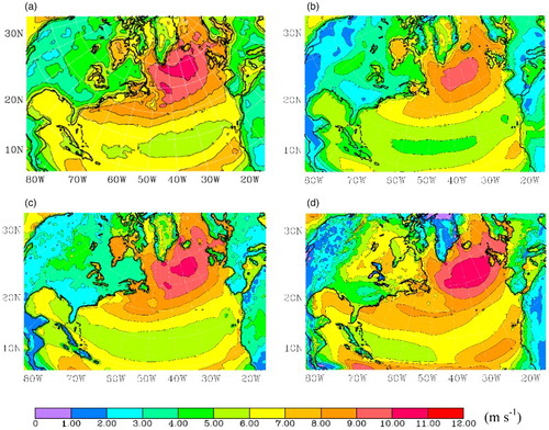
Fig. 1 The seasonal mean of 6-hourly 10 m wind speed (m s⁻¹): (a) QSCAT/NCEP, (b) ERA-40, (c) CFSR, and (d) CRCM.

For our study, simulation of a 30-year period from 1970 to 1999 is performed to represent the present climate, with the initial and lateral boundary conditions taken from CGCM3 outputs; these years represent the last tri-decadal period of the IPCC (2007) twentieth century simulations for the years 1850–2000. The Special Report on Emissions Scenarios (SRES) A1B climate change experiment is for the years 2001–2100, initialized from the end of the twentieth century climate simulations (IPCC, 2007; Solomon et al., 2007). Therefore, to investigate the influences of different scenarios, we compare later tri-decadal periods to the present climate given by 1970–1999. The SRES A1B scenario is marked by very high economic growth and a convergence of socioeconomic conditions. This scenario is a “middle usage” of the energy sources whereby CO₂ concentrations will likely reach 720 ppm by 2100 (Nakićenović & Swart 2000). The future climate change is represented by a CRCM simulation of the 30-year period from 2040 to 2069, also driven by CGCM3 outputs and the A1B scenario. The WW3 wave model is driven by the 10 m winds and ice cover, which are linearly interpolated in space to match the wave model grid every 6 hours. For this study, the autumn wave climate is represented by the 2-month period from 1 September to 31 October.

b Wave Model

We used the WW3 wave model (version 3.14), which is a third-generation spectral model, for ocean surface gravity waves, as described by Tolman (2009), with the usual source terms, such as energy input by wind, wave dissipation, non-linear wave–wave interactions, and bottom dissipation parameterizations. The model domain is the North Atlantic (20°N–70°N, 82°W–18°E). The wave model grid spacing is 0.5° × 0.5°, and the spectral domain is divided into 29 frequency and 24 directional bins (15°). Binned frequencies range from 0.035 to 0.6 Hz using an increment factor of 1.07. Wave simulations are driven by CRCM winds from 27 August to 31 October for each year during 1970–1999 and 2040–2069, allowing the first five days as spin-up time for the model. Hereafter, this dataset is denoted CRCM-w.

c ERA-40 Wave Reanalysis

The ERA-40 reanalysis data were produced by ECMWF's Integrated Forecasting System, incorporating a coupled atmosphere–wave model and data assimilation (Simmons, 2001; Uppala et al., 2005). The dataset is given on a 2.5° × 2.5° latitude/longitude grid covering the entire globe from September 1957 to August 2002, including variables such as SWH, mean wave period, and mean wave direction. This continuous 45-year period makes it suitable for studying wave climate variability and estimating the climatology of specific wave parameters. Our initial concern is verification of our simulation of the present wave climate produced by WW3. As a baseline, we compare our results to those of the ERA-40 wave dataset. However, Caires and Sterl (2003) found that ERA-40 underestimates the highest wind speeds for the present climate, which thus also affects its wave climate.

d CFSR Winds and its Wave Hindcast

The capability of our model results to represent the present climate is also assessed by comparing our results with the wave climate resulting from CFSR reanalysis winds. The CFSR dataset is generated by NCEP, using a spectral atmospheric model (Saha et al., 2006) at T382 resolution (38 km) with 64 hybrid vertical levels and the Modular Ocean Model, version 4p0d, from the Geophysical Fluid Dynamics Laboratory (Griffies, Harrison, Pacanowski, & Rosati, 2004). The CFSR winds at the 10 m reference height were used to generate an associated wave climate using WW3. The winds are at 6-hourly intervals and 1/2° spatial resolution over the same simulation domain as described in Section 2b. Thus, a 21-year hindcast was provided for SWH, mean wave period, mean wave direction, peak period (T_p), and mean direction at the peak period, with 1/2° spatial resolution from 1979 to 1999. Hereafter, this wave dataset is denoted CFSR-w. The comparisons were made between the CRCM winds and CRCM-w waves (1979–1999) and CFSR winds and CFSR-w waves (1979–1999).

e Storm Detection Methodology

A two-step system, adapted from an earlier work by Long et al. (2009), is used to detect and track storms automatically in this study. The cyclone detection algorithm begins by searching the grid points for a relative minimum of mean sea level pressure (MSLP). For a given initial array area of 11 × 11 grid points (∼500 km × 500 km), the criterion is that a candidate cyclone must have a minimum pressure lower than 1010 hPa. However, MSLP cannot be the sole criterion for determination of cyclones because other factors can influence MSLP's use in storm-track determination. For example, complicating factors can be related to the tendency for storm tracks to shift to regions with preferentially lower pressure in a warmer climate. Thus, vorticity is also used because vorticity is less influenced by large-scale background changes (Anderson, Hodges, & Hoskins, 2003; Hoskins & Hodges, 2002; Sinclair & Watterson, 1999). Therefore, we require that a candidate cyclone also have a local maximum of relative vorticity at the 850 hPa level, within a specified distance (five grid points, ∼200 km) from the MSLP minimum.

After a database of snapshots of potential storms is created satisfying the above conditions, a simple nearest neighbour search is used to track the individual cyclones from the preceding (6 h) “time steps.” If a cyclone falls within 800 km of a previously identified cyclone from a preceding time step, it is assumed to be a continuation of the previous cyclone. Otherwise, it is considered a new cyclone. A candidate storm is required to have a lifetime of at least 24 h in order to be considered viable.

f Student's t-test

The Student's t-test is used to determine whether the differences between the two sets of data are statistically significant and can be written as follows:

where and are the means; and are the standard deviations, which have sample sizes n₁ and , respectively. For a given significance level , if the absolute value of the value is above the critical t-test value , the differences between the two datasets are significant at that level with + -2 degrees of freedom.

3 Present climate

a Wind Fields

One of the important uncertainties in climate change projections of the wave climate is the variability in wind forcing. Therefore, the first priority is to examine the 10 m winds in our simulation of the present climate. Figure 1 presents the average of 6-hourly 10 m wind fields for the present autumn climate, as represented by 21 years (1979–1999) for ERA-40, CRCM, and CFSR, and a somewhat delayed 10 years (1999–2008) of available data for QSCAT/NCEP blended winds. In this comparison, the maximum winds appear in the high-latitude areas of the Northeast Atlantic in all these climate datasets.

Figure 1a shows the QSCAT/NCEP blended winds. An important feature of these wind data is that they contain high-wavenumber (spatial) information from QuikSCAT measurements and, therefore, contain more highly resolved spatial information than the ERA-40 data or the other wind data displayed in Fig. 1. The ERA-40 winds are presented in Fig. 1b, and CFSR winds are presented in Fig. 1c. Compared with QSCAT/NCEP winds, ERA-40 winds appear to be underestimated, whereas the CFSR winds are in general agreement. Winds from the CRCM simulation are given in Fig. 1d and appear to be generally consistent with the QSCAT/NCEP winds over the Northeast Atlantic although they are weaker in the northwestern area off the North American east coast by about 1 m s⁻¹. Moreover, spatial details, such as the well-known tip-jet winds off the southern end of Greenland, and coastal features, such as the winds over the Gulf of St. Lawrence coastland areas seen in QSCAT/ NCEP winds, are better reproduced by CFSR and CRCM simulations than by ERA-40.

Figure 2 presents the highest 10% wind speeds for the wind data shown in Fig. 1. Here, we define extreme wind speed as the average of the highest 10% of the 6-hourly 10 m wind speeds for each autumn, following the approach of Sasaki, Iwasaki, Matsuura, and Iizuka (2005). These winds are hereafter denoted Wtop10. A prominent feature of the QSCAT/NCEP data (Fig. 2a) is that the strongest winds occur at high latitudes, particularly the Greenland tip jet (Moore, 2003; Moore & Renfrew, 2005; Pickart, Spall, Ribergaard, Moore, & Milliff, 2003; Våge, Spengler, Davies, & Pickart, 2009) and over waters off the southeast coast of Greenland. Qualitatively, CFSR and CRCM reproduce patterns that are similar to those from QSCAT/NCEP. However, consistent with Caires and Sterl (2003), we find that the Wtop10 values from ERA-40 appear to underestimate those shown in the QSCAT/NCEP data (Fig. 2b). A possible reason for this is that the relatively coarse resolution of the ERA-40 data cannot represent the small spatial distribution features off Greenland's southern tip.

Fig. 2 The mean of 10% strongest 6-hourly 10 m wind speed (m s⁻¹): (a) QSCAT/NCEP, (b) ERA-40, (c) CFSR, and (d) CRCM.

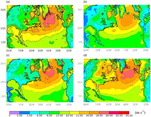
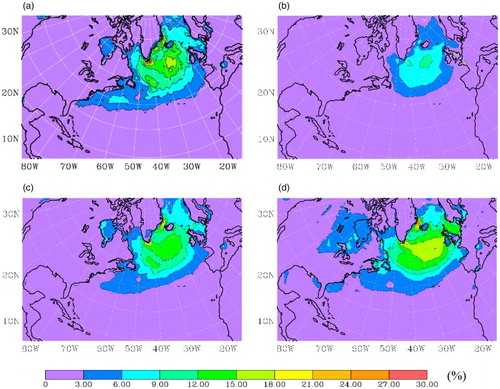
As an alternative representation, we calculate the frequency of occurrence of 6-hourly winds greater than 15 m s⁻¹, shown in Fig. 3. Once again, it is shown that CFSR and CRCM can capture the high wind spatial and temporal distributions suggested by the QSCAT/NCEP data, specifically in the Northeast Atlantic, with a frequency of occurrence that is more than 15%. However, in the Northwest Atlantic, the CRCM winds appear to be underestimated compared with QSCAT/NCEP data (Fig. 3d), suggesting a reduced storm-track density for this region. Also, the ERA-40 data again appear to underestimate the strongest winds (Fig. 3b).

Fig. 3 The frequency (%) of 6-hourly 10 m wind speed ≥15 m s⁻¹: (a) QSCAT/NCEP, (b) ERA-40, (c) CFSR, and (d) CRCM.

b Storm Climates

We apply the methodology for cyclone detection and tracking described in Section 2e, to estimate the distributions of the storm-track densities. Figure 4 presents storm-track densities calculated by counting the number of storm tracks that pass through each 1000 km × 1000 km box. The cyclone numbers are determined by counting the cyclone occurrences that are connected to their trajectories. Each cyclone is counted just once, per track, per grid point. Thus multi-counting at a given grid point is avoided. Results shown in Fig. 4 are for the months of September and October, averaged over 21 years (1979–1999). We also include NCEP/NCAR reanalysis data (Kalnay et al., 1996) in this comparison.

Fig. 4 Storm-track densities (1 yr⁻¹) averaged over the present climate period from (a) ERA-40, (b) NCEP, (c) CFSR, and (d) CRCM.

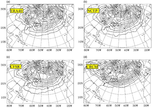
The highest density of storm events tends to occur off the southeast coast of Greenland, just south of Iceland, in proximity to the centre of the Icelandic Low, as suggested by the three reanalysis datasets, ERA-40, NCEP, and CFSR (Figs 4a–4c) and by the CRCM results (Fig. 4d). The dominant North Atlantic storm tracks are reflected in these datasets although results from CRCM exhibit a low bias in the southeastern part of the North Atlantic, in coastal waters off the North American east coast (from Florida to Chesapeake Bay), suggesting the model domain and set-up does not capture the initial storm tracks of extra-tropical hurricanes and cyclones well in their subtropical genesis region.

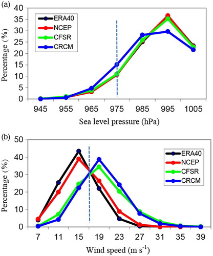
Corresponding estimates for the distribution of storm intensity are shown in Fig. 5 for minimum SLP and maximum wind speed, . Thus, the percentage of storms with minimum SLP less than 975 hPa is approximately 21% for CRCM, which is higher than results for the three reanalysis datasets (NCEP, CFSR, and ERA-40), approximately 14%, 15%, and 14%, respectively, in this category. In the most populated segment of the distribution, 985–1005 hPa, the portion of storms in the CRCM simulation is lower than corresponding results in the NCEP, CFSR, and ERA-40 datasets. Figure 5b shows storm distributions in terms of maximum wind speed. Here, the maximum wind speed is defined as the highest wind speed within a distance of 1000 km from the cyclone centre. As before, we find that the highest winds (above ∼17 m s⁻¹) are biased low in the ERA-40 data compared with CFSR and the results from other datasets. Moreover, it is apparent that both NCEP and ERA-40 appear to be biased low compared with CFSR results for densities of the most intense storms; a possible cause is their relatively coarse resolutions. This finding is consistent with Caires, Sterl, Bidlot, Graham, and Swail (2004), who point out that the ERA-40 data tend to underestimate SWH at high wind speeds. By comparison, CRCM achieves a distribution of storms with maximum wind speeds that are in good agreement with CFSR results.

Fig. 5 (a) Frequency (%) of storms as a function of minimum MSLP (hPa) for present climate (1979–1999) cyclones from ERA-40, NCEP, CFSR, and CRCM over the CRCM domain; (b) frequency (%) of storms as a function of maximum 10 m wind speed (m s⁻¹).

c Wave Climate

The autumn wave climate, represented in terms of the mean distributions of 6-hourly SWHs for September and October are shown in Figs 6a–6c. These figures give a visualization of the WW3 domain, defined in Section 2b. Thus, for the boreal fall, the mean SWH is characterized by high waves at high latitudes in the northeast region of the North Atlantic. The maximum seasonal mean SWH is approximately 2.5 m when WW3 is driven by ERA-40 winds (Fig. 6a), compared with approximately 3.5 m in results from CFSR-w (Fig. 6b) and approximately 4 m in results driven by CRCM winds (Fig. 6c). Results from CRCM-w are similar to those of CFSR-w and stronger than those of ERA-40, reflecting the respective characteristics of the winds.

Fig. 6 Seasonal mean SWH (m) from (a) ERA-40, (b) CFSR-w, and (c) CRCM-w; 10% strongest SWH (m) from (d) ERA-40, (e) CFSR-w, and (f) CRCM-w. The contour intervals are 0.5 m for (a)–(c), and 1 m for (d)–(f).

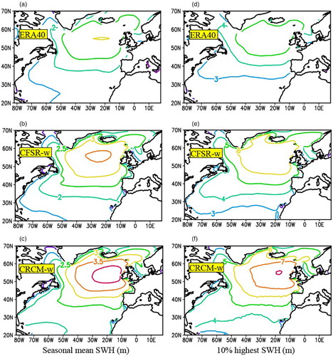
We also consider the autumn extreme SWH fields, defined as the average of the highest 10% of the SWH results for each autumn (hereafter Htop10). These results are shown in Figs 6d–6f. The simulated maximum Htop10 is approximately 8 m for WW3 results driven by CRCM, which is stronger than those from ERA-40 at 5 m or from CFSR-w at about 7 m. Qualitatively, Htop10 patterns for CRCM-w are more similar to those of CFSR-w than those produced by ERA-40. For example, similar features for the former two datasets occur in waters off eastern Canada; around the Gulf of St. Lawrence; Newfoundland and Labrador; the Labrador Sea; in waters off Greenland, especially the southern tip; and the northeast North Atlantic, between Iceland and Europe. These SWH similarities follow the spatial patterns for the 10% strongest winds, denoted Wtop10, and frequencies of high winds (> 15 m s⁻¹) in Figs 2 and 3.

The mean wave direction and mean wave period T_m are additional notable wave parameters, shown in Fig. 7. The mean wave directions tend to be easterly at low latitudes, southerly over mid-latitudes near North America and also at very high latitudes, and westerly in the northeast North Atlantic, near Europe. Again, as in the results for Htop10, mean wave direction results from CRCM-w are qualitatively more comparable to those of CFSR-w than to results from ERA-40. This is evident at lower latitudes in waters off eastern Canada, the Gulf of St. Lawrence, Newfoundland and Labrador, the Labrador Sea, waters around Greenland, and the northeast North Atlantic between Iceland and Europe, where the differences are no more than 10°. In particular, mean wave directions in the mid-latitudes are more westerly in results from CRCM-w and CFSR-w, than in the results of ERA-40.

Fig. 7 Seasonal mean wave direction (^o): (a) ERA-40, (b) CFSR-w, and (c) CRCM-w. Seasonal mean wave period(s) in (d) ERA-40, (e) CFSR-w, and (f) CRCM-w. The contour intervals are 30^o for (a)–(c), and 0.5 s for (d)–(f).

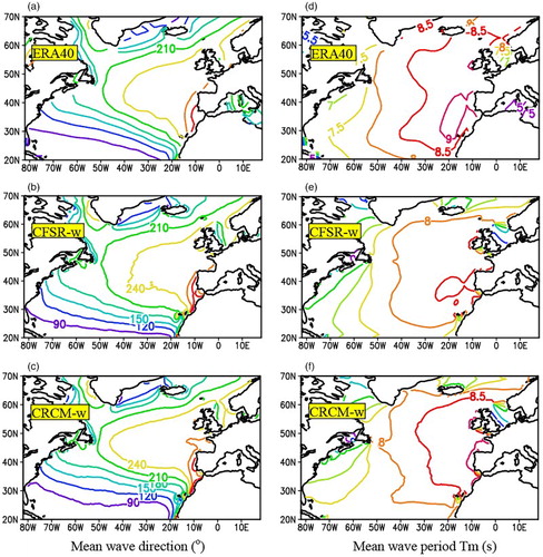
The mean wave period T_m is important for design criteria for offshore structures. Figure 7d shows the mean wave period in ERA-40, featuring a dominant centre for long wave periods in the eastern portion of the North Atlantic and shorter periods in the Northwest Atlantic, for example, in coastal areas of the eastern North American seaboard and the Labrador Sea. Although qualitatively similar to ERA-40, results from CRCM (Fig. 7f) suggest larger values (∼9 s) for T_m in the Northeast Atlantic, in coastal areas off Europe, and relatively smaller values (∼5 s) in the western part of the North Atlantic. Results from CRCM-w appear to be intermediate between those of ERA-40 and CFSR-w. In terms of overall patterns, the WW3 results driven by CRCM are generally more consistent with the T_m climatology generated by CFSR winds than those suggested by ERA-40.

d Wave Regimes

Ocean surface gravity waves may generally be categorized as belonging to three regimes: swell, mixed seas (or intermediate seas), and wind-sea. Swell can be distinguished from wind-sea in terms of criteria such as wave steepness or wave age. Following Charles, Idier, Delecluse, Déqué, and Le Cozaanet (2012) and Hanley, Belcher, and Sullivan (2010), our criteria are based on inverse wave age, , which may be defined as: (1)

where the phase speed at the spectral peak is , the local wind speed at 10 m height is , the mean wave direction is , and the local wind direction is . Following this approach, the three basic wave regimes may be specified as: (2) (3) (4)

As well as being an indicator of the wind-wave regime, inverse wave age can also be a good indicator of the degree of coupling between the wind and the waves: for higher values of the inverse wave age, the waves are younger and, therefore, tend to be more strongly coupled to the wind (Hanley et al., 2010). For consideration of wave regimes, the required spectral peak wave parameters are available from CFSR-w and CRCM-w results but not from ERA-40 data per se.

Distributions of inverse wave age, , are shown in Figs 8a and 8b. These results suggest that relatively higher values of appear in the more northern part of the Northwest and Northeast Atlantic, along the area of mid-latitude storm tracks, especially in semi-enclosed seas, suggesting actively generating and developing young waves and wind-sea dominant conditions. In these areas, values of are limited by the effective fetch associated with evolving storm tracks in both CFSR-w and CRCM-w datasets. In the most stormy areas, the differences between and are only a few metres per second, and rapidly developing storm conditions induce the generation of young developing waves with concomitant high values for the inverse wave age. Outside the areas of the highest density of storms and storm tracks, where values for are lower, waves are older and more mature, and the inverse wave age is also generally reduced, with the lowest values occurring on the eastern side of the North Atlantic basin, where is highest, suggesting the longest spectral peak periods. Moreover, for the region between 20°N and 40°N, east of the North Atlantic storm-track area corresponding to relatively lower wind speeds, the inverse wave age is also generally relatively low, as indicated by the CFSR-w results. Results from CRCM can capture the overall characteristics of the inverse wave age given by CFSR-w results although the former has slightly lower values over the Northwest Atlantic storm-track area and higher values in the southeast region over lower latitudes (Fig. 8b).

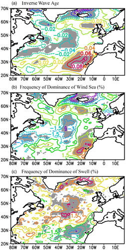
Fig. 8 Seasonal mean inverse wave age in (a) CFSR-w and (b) CRCM-w; the frequency (%) of occurrence of wind-driven waves in results from (c) CFSR-w and (d) CRCM-w; and the frequency (%) of occurrence of swell from (e) CFSR-w and (f) CRCM-w.

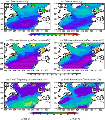
Results from both CFSR-w and CRCM-w (Figs 8a and 8b), over most of the open ocean, exhibit large areas where inverse wave age estimates do not correspond to dominance by either the wind-sea regime (>0.83) or the swell regime (<0.15). This implies that the sea state is mixed, that is, composed of both wave types. However, it is interesting to distinguish which ocean areas are dominated by either wind-sea or swell. Figures 8c and 8d suggest that wind-sea occurs most frequently, apparently more than 20% of the time, in high latitudes of the Northwest Atlantic (e.g., the main storm-track region) and to the northwest of the main storm-track region. The resulting swell waves generated by these storms propagate across the North Atlantic, including southward and eastward areas and tend to be dominant in the southeastern area, where storm generation is relatively less common. Specifically, Figs 8e and 8f suggest that in the eastern portion of the region, between 20° and 40°N, where spectral wave peaks are high, values for are high, is low, and the swell frequency is at least 15% in results from both CFSR-w and CRCM-w. Because wind speeds are generally stronger in CRCM results than in CFSR results, in both the Northwest and the Northeast Atlantic (Fig. 3), the frequency of occurrence of wind-sea dominance in CRCM-w results tends to be higher than in CFSR-w results, particularly in the storm-track areas of the North Atlantic, and the frequency of occurrence of dominance in swell in CRCM-w results tends to be lower than in CFSR-w results (Figs 8e and 8f).

4 Climate change impacts

a Wind

In the future climate scenario, simulated changes in winds can be seen over the entire North Atlantic relative to the present climate mean winds (Fig. 9). Averaged over our entire domain, the mean wind speed is about 6.5 m s⁻¹ and for the 10% strongest wind speeds, also denoted Wtop10, it is 13.0 m s⁻¹ during the 1970–1999 period. For the future climate scenario (2040–2069), mean winds reach essentially the same value, 6.5 m s⁻¹, and Wtop10 reaches 12.9 m s⁻¹.

Fig. 9 Estimates from CRCM. (a) Difference in mean 6-hourly 10 m wind speed (m s⁻¹) and (b) difference in 10% strongest 6-hourly 10 m wind speed (m s⁻¹) for the future climate scenario minus the present climate. The contour interval is 0.3 m s⁻¹ for (a) and 0.5 m s⁻¹ for (b). The grey shading indicates the 90% significance level from a Student's t-test.

Compared with the present climate, weakening wind speeds are observed over the mid-latitudes. Specifically, projected decreases of approximately 0.8 m s⁻¹ are estimated in mean wind speed and as much as 1 m s⁻¹ in Wtop10. The winds increase over high latitudes and in the Northeast Atlantic, with a projected increase of approximately 0.3 m s⁻¹ in the mean wind speed and 0.5 m s⁻¹ in Wtop10. Moderate weakening occurs in the winds in the far Northwest Atlantic and also in the Labrador Sea region, by about 0.6 m s⁻¹ in the mean winds and about 0.2 m s⁻¹ in Wtop10.

b Storm Climate

The changes in winds and wave heights over the North Atlantic reflect the associated changes in storm climate, specifically changes in storm frequency, track, and intensity. These changes are related to changes in the atmospheric circulation.

Under the A1B scenario, the CRCM simulated total cyclone population decreases in the future by 2.5%, but intense cyclones (with central pressures <980 hPa) increase by about 12%. This result is consistent with that of Lambert and Fyfe (2006). Based on different GCMs and results from different IPCC scenarios, they found that the total number of winter cyclones will decrease in the northern and southern hemispheres, whereas the number of the most intense winter cyclones (less than 960 hPa) will increase. Our results also suggest that the number of intense cyclones (defined in terms of wind speed >25 m s⁻¹) will increase in the future climate scenario. Figure 10 estimates the distributions of the total cyclones and the most intense cyclones in the future climate scenario. Differences are also presented, comparing the present populations with the impacts of climate change, showing the changes in cyclone frequencies, tracks and intensities.

Fig. 10 Cyclone track densities from CRCM. Difference between future climate and present climate for (a) total cyclone track densities, (b) intense cyclone densities (MSLP ≤ 970 hPa), and (c) intense cyclone densities defined in terms of winds (>27 m s⁻¹). Densities are in units of 1 yr⁻¹. Grey shading indicates the 90% significance level from a Student's t-test. The contour intervals are 0.2 yr⁻¹ for (a)–(c).

Under the A1B climate change scenario, the CRCM simulation appears to indicate increases in storm frequencies over the area north of approximately 50°N, including the Northeast Atlantic, waters around Greenland, and the Labrador Sea, and decreases over much of the mid-latitude North Atlantic (Fig. 10a). Changes in the distribution of the most intense cyclones (minimum MSLP ≤970 hPa) suggested in Fig. 10b include increases in cyclone frequency in waters east of Greenland and the Northeast Atlantic and reductions over much of the remaining areas, including mid-latitude areas and the Labrador Sea. Similar results are obtained when the most intense cyclones are identified in terms of winds (Fig. 10c).

c Impact of the Steering Flow

The change in storm densities is probably a result of changes in the steering flow (mean climatological flow) in the future climate scenario. Figure 11 shows the impacts of climate change on the 200 hPa westerly wind speed and relative vorticity, as simulated by the CRCM. In the future climate scenario, the upper westerly jet stream is stronger and farther north than in the present climate. This result is consistent with Fyfe (2003) and Jiang and Perrie (2007). The latter suggest that cyclones whose tracks are most closely oriented with the upper westerly jet will be the most affected by climate change.

Fig. 11 CRCM simulation of 200 hPa mean westerly winds and jet (m s⁻¹) showing (a) present climate, (b) future climate, (c) difference between future climate and present climate. Also, mean relative vorticity (10⁻⁵ s⁻¹) results are shown: (d) present climate, (e) future climate, and (f) difference between future and present climate. Grey shading in (c) and (f) indicates the 90% significance level from a Student's t-test. The black solid and dashed lines in (a) to (c) indicate the locations of maximum wind for each longitude for the present and future climates, respectively. The contour intervals are 5 m s⁻¹ for (a) and (b), 0.5 m s⁻¹ for (c), and 0.2 10⁻⁵s⁻¹ for (f).

Corresponding results are shown in Fig. 11d for relative vorticity at 200 hPa. In the climate change scenario, the relative vorticity becomes stronger and is extended westward and northward, with decreasing magnitudes over mid-latitude areas. Therefore, the overall storm density also tends to be extended and to increase in northern areas and decrease over mid-latitudes (Fig. 10). Changes in storm characteristics have a direct influence on winds and, therefore, on waves, particularly for changes in cyclone frequency, intensity, and tracks. These changes suggest that the impact of feedbacks between the ocean surface and the upper atmospheric mean climatological flow could be important (Jiang & Perrie, 2007) and that they also can influence the wave climate, accordingly.

d Waves

The projected changes in the autumn wave climate are indicated in Figs 12–14. Under the A1B climate change scenario, the mean SWH appears to increase by approximately 0.1 m over the Northeast Atlantic, and associated decreases occur in the mid-latitudes and subtropics. For the mean of the 10% strongest SWH, also denoted Htop10, the increases are about +0.5 m in the northeast North Atlantic, with decreases of as much as −0.6 m in the mid-latitudes, particularly in the eastern portion near Europe, and also in the subtropics. Similar results were found by Wang, Zwiers, and Swail (2004) using coarser-resolution CGCM2 projections, although not quite as strong. Averaged over our entire North Atlantic domain, the mean SWH is 2.52 m in 1970–1999 and shows little change over the next several decades, reaching only 2.39 m by 2040–2069. By comparison, the corresponding mean for Htop10 is about 5.01 m, for 1970–1999 and decreases to 4.78 m in the future climate scenario. Therefore, the projected changes in winds are reflected in the changes in mean wind-driven SWH and also in Htop10. Notably, the increases in the strongest waves in the Northeast Atlantic occupy large areas of the open ocean (Fig. 12b).

Fig. 12 Differences between future climate scenario and present climate for (a) mean SWH (m) and (b) 10% strongest SWH (m). The contour interval is 0.1 m for (a) and 0.2 m for (b). The grey shading indicates the 90% significance level from a Student's t-test.

Fig. 13 Differences between future climate scenario and present climate for (a) mean wave direction (^o) and (b) mean wave period (s). The contour interval is 5^o for (a) and 0.05s for (b). The grey shading indicates the 90% significance level from a Student's t-test.

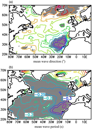
Fig. 14 Differences between future climate scenario and present climate for (a) mean inverse wave age, (b) frequency (%) of dominance of wind-driven waves, and (c) frequency (%) of dominance of swell. The contour interval is 0.02 for (a) and 1.5% for (b) and (c). Grey shading indicates the 90% significance level from a Student's t-test.

Connected with the northward shift of the overall winds climate, the mean wave directions tend to become more westerly over the northern North Atlantic and more easterly over the southern North Atlantic, as shown in Fig. 13a. These changes in mean wave direction reflect the changes in storm intensity and storm tracks and are related to changes in winds, discussed in the previous section.

The impacts of projected climate change on waves should also be reflected in changes to the mean spectral frequency or mean wave periods. Changes in mean wave periods are presented in Fig. 13b. The apparent effect of climate change is to reduce mean wave periods (higher mean peak frequencies) over most of the mid-latitude North Atlantic. The statistical significance is high for most of this area. Conversely, increased mean wave periods of approximately 0.2 s are projected for the climate change impacts in the far Northeast Atlantic corresponding to regions of increased wave heights.

e Wave Regimes

Estimated changes in swell, mixed seas, and wind-generated waves (or wind-sea) are shown in Fig. 14. In particular, Fig. 14a presents the corresponding changes in the inverse wave age under the future climate scenario, showing that in regions where the winds increase and the strongest waves increase (Figs 9 and 12), the inverse wave age, , also tends to increase. These areas include the subtropics from about 20° to 35°N, and the Northeast Atlantic between Europe and Iceland. These are areas of relatively young, rapidly developing waves, related to enhanced storm development. Other areas, such as the mid-latitudes across much of the North Atlantic, experience a slight reduction in , suggesting older waves related to slightly lower winds and waves (Figs 9 and 12), associated with reduced storm development activity and a northward shifting of the dominant storm tracks.

Following the discussion in Section 3d, Fig. 14 suggests the impacts of climate change on the frequency of occurrence of wind-driven waves, mixed seas, and swell. Consistent with the changes in winds and waves in Figs 9 and 12, the suggested changes are reductions in the frequency of dominance of wind–sea in mid-latitudes for most of the North Atlantic and increases in these frequencies in the Northeast Atlantic, between Europe and Iceland, in the subtropics, particularly the eastern portion near Africa, with some changes occurring in the southern Labrador Sea, south of Greenland. As in Section 3d, changes in frequency of dominance of wind-sea appear to correspond to opposite changes in the frequencies of dominance of swell (Figs 8d and 8f). Thus, climate change appears to cause the frequency of occurrence of swell dominance to increase across much of the North Atlantic mid-latitudes and decrease in the far Northeast Atlantic (Fig. 14c). Lower winds in areas like the mid-latitudes imply that swell is more prevalent in the future climate.

5 Discussion

The first requirement for a study on climate change for waves is to establish that the simulated winds are reliable for the present climate. Biases in the model winds directly result in biases in the waves. For autumn (September and October) in the North Atlantic, we have demonstrated that the CRCM winds are reliable by comparing them with accepted high-quality reanalysis wind data, specifically with the QSCAT/NCEP blended wind data and the CFSR reanalysis data. In fact, the CRCM winds compare better with the QSCAT/NCEP blended wind data and the CFSR reanalysis data than with winds from ERA-40 data or NCEP reanalysis data (not shown). Comparisons include mean distributions of wind speeds, 10% strongest winds (denoted Wtop10), and frequency and distribution of mean wind speeds averaged over the present climate.

Wave climate estimates, as provided by WW3 driven by CRCM winds, were shown to be reliable, compared with those generated from CFSR wind data and better than those resulting from ERA-40 wind data. In addition to SWH, averaged over the present climate represented as 1979–1999, comparisons also considered distributions of the 10% highest wave climate estimates, as well as spectral parameters such as mean wave directions and periods. To provide estimates of spatial distributions of wind-sea and swell wave regimes, mean inverse wave age estimates were made, resulting from WW3 driven by CRCM; these results were shown to compare reasonably well with those resulting from CFSR winds. Associated estimates of the frequency of occurrence of wind-sea regimes compared with swell were also made.

In this study, we identified and selected storms by applying an automated storm detection/tracking algorithm for the present climate (1970–1999) and future climate (2040–2069). In terms of the storm climatology, the CRCM simulation agrees reasonably well with the results from the reanalysis datasets considered in this study. Comparisons included spatial densities of autumn storms averaged over the present climate and histograms of storm distributions as a function of MSLP and wind speeds. However, the CRCM results tend to exhibit biases in cyclone density along the North American east coast, particularly from around Florida to the Chesapeake Bay area. On the other hand, because of their relatively coarse resolution, both NCEP and ERA-40 have difficulties resolving intense storms, and the maximum wave heights in their wave climates tend to be underestimated.

Compared with the present climate, the A1B climate change scenario results suggest that mean autumn winds tend to increase over the Northeast Atlantic between Greenland and Europe, as well as in the eastern portion of the subtropics, particularly near Africa, and decrease over much of the mid-latitudes and the Northwest Atlantic including the Labrador Sea. These latter results appear to be statistically significant. Moreover, for autumn, the mean Wtop10 give essentially the same result: an increasing tendency in the Northeast Atlantic and eastern subtropics, particularly off Africa, and slight decreases in the mid-latitudes and elsewhere.

Compared with the present climate, increases in the mean SWH appear over the Northeast Atlantic, and associated decreases are suggested for the subtropics and also for the western North Atlantic, off eastern Canada, and the United States. Although winds may appear to increase in the subtropics off the coasts of Africa, they are easterlies; fetches are relatively very short, and the effects on SWH are not substantial. In terms of the mean 10% highest SWH, denoted Htop10, the impacts of climate change are similar to the changes in the entire mean SWH dataset, except that the largest increases are suggested for the Northeast Atlantic.

In terms of the mean wave direction, the impacts of climate change appear to result in a slight “turning” of the dominant orientation of the overall sea state. Mean wave directions tend to become more westerly over the northern North Atlantic and become more easterly over the southern North Atlantic. In terms of mean wave period, the impact of climate change appears to increase mean wave periods over the Northeast Atlantic, in association with enhanced winds, ongoing wave development, and higher sea states. Mostly decreased mean wave periods occur elsewhere, coinciding with wind changes, reduced wave development, as well as lower sea states, and swell dominance.

In terms of associated mean inverse wave age, the impacts of climate change suggest increased wave ages in the Northeast Atlantic and the subtropics, particularly off the coast of Africa, in the same areas where winds tend to increase and where wave generation continues to increase. Much of the rest of the Atlantic, particularly the mid-latitudes, experience reduced values for mean inverse wave age, where mean winds tend to be diminished and where the prevalent characteristic of the mean wave fields tends to be swell regimes. These characteristics are approximated by using inverse wave age as an indicator of the dominance of the balance between wind-sea and swell, with sufficiently low values identified as swell, sufficiently high values as wind-sea, and intermediate values as mixed seas.

Thus, we investigated the possible impacts of climate change scenario A1B on autumn winds and waves. But what is the mechanism for these impacts? Changes in winds reflect changes in the autumn storm climate, particularly for the most severe storms. Changes in the storm climatology are in response to large-scale changes in the autumn climatological streamflow. The occurrence of increases in the most intense cyclones is a response to a warmer climate change scenario, especially over the Northeast Atlantic. However, over the mid-latitudes of the North Atlantic, consistent with a northward shift of storm tracks, we also find that the autumn storm density decreases in the future climate change scenario, both for the total storm population and also for the most intense storms. Associated with changes in storm activity, the 10 m winds, the Wtop10, and the severe storms appear to decrease over the mid-latitudes and increase over the Northeast Atlantic in autumn in the climate change scenario.

The suggested change in storm tracks is related to the background atmospheric streamflow (Mizuta, Matsueda, Endo, & Yukimoto, 2011; Yin, 2005). In the climate change scenario, it is evident that the upper westerly jet stream is somewhat stronger and farther north than in the present climate. The corresponding relative vorticity at 200 hPa is projected to increase over the high-latitude area and decrease over the mid-latitudes, which will influence the storm climate (Fig. 11). Moreover, results from the climate change scenario suggest an increase in relative vorticity, which tends to occur in upstream regions of cyclone trajectories, potentially inducing an increased population of the most intense cyclones in the downstream area, which is the Northeast Atlantic.

A bias in the CRCM results is the underestimated SWHs for the mid-latitudes on the west side of the North Atlantic, off the coast of the United States, compared with the reanalysis data. Part of this bias may occur because of uncertainties in forcing data (CGCM3) or in differences among A1B climate scenario ensemble members (Teng, Washington, & Meehl, 2008). Additional uncertainties in the regional climate change simulations can also result from alternative future emissions scenarios, for example RCP8.5. Therefore, more CRCM simulations and ensemble members, as well as different climate change simulations, are needed to achieve a more robust ensemble of possible climate change estimates. Thus, we will pursue additional ensemble simulations of climate change scenarios for winds and waves in ongoing research.

6 Conclusions

In this study we investigated the influence of climate change on North Atlantic storms, winds, and waves. The A1B climate change scenario, as simulated by CGCM3, is used to drive the CRCM, thereby providing dynamically downscaled winds to drive the wave model, WW3. The study area is a limited area domain covering the North Atlantic, comparing present climate conditions, represented by the 1970–1999 period, to a future climate scenario for the 2040–2069 period. Autumn storms, winds, and waves occurring in September and October were considered.

Under the climate change scenario, the total number of cyclones is estimated to decrease in the future by about 2.5%, but the intense cyclones (central pressure <980 hPa or winds >25 m s⁻¹) increase by about 12%. Increases in storm frequency occur in areas north of approximately 50°N, in the Northeast Atlantic, around Greenland and the Labrador Sea, and decreases in the mid-latitudes. In terms of winds, no essential climate change impact is expected for mean winds (∼6.5 m s⁻¹) or the 10% strongest mean winds (∼13 m s⁻¹) averaged over the entire North Atlantic. However, there are spatial variations. Over the mid-latitudes, decreases as a result of climate change are approximately 0.8 m s⁻¹ for mean winds and as much as 1 m s⁻¹ for Wtop10, whereas over the high-latitude Northeast Atlantic, projected increases in mean winds are about 0.3 m s⁻¹ and for Wtop10, 0.5 m s⁻¹. Moderate weakening appears to occur in the far Northwest Atlantic and the Labrador Sea, by 0.6 m s⁻¹ in mean winds and 0.2 m s⁻¹ in Wtop10. These changes in storms are related to the overall northward shift of the climate system in a warmer climate.

In terms of corresponding waves, the climate change scenario appears to increase mean SWH in the Northeast Atlantic by 0.5 m for Htop10, with decreases elsewhere by as much as 0.6 m in the mid-latitudes and subtropics. No notable changes are suggested for mean SWH, averaged over the entire North Atlantic, which is 2.5 m in the present climate and 2.4 m in the future climate. For Htop10, the overall North Atlantic average is suggested to decrease from 5.0 m in the present climate to 4.8 m in the future scenario. Corresponding mean wave directions also change, reflecting changes in storms and winds, tending to become more westerly over northern latitudes and more easterly over southern latitudes. Mean wave periods are projected to increase in far northeastern areas and decrease elsewhere.

Enhanced autumn storminess is projected to occur in the Northeast Atlantic, where winds and waves also tend to increase, with increased young rapidly developing waves. This is suggested by increased inverse wave age in these areas, whereas the mid-latitudes and other areas experience inverse wave age reductions, suggesting older waves associated with reduced winds and storm activity. In the same manner, climate change is expected to cause reductions in the frequency of wind–sea dominance in the mid-latitudes, increases in the far Northeast Atlantic, and appropriate opposite tendencies for swell dominances.

Acknowledgements

We thank Michel Giguère at Ouranos for many helpful discussions about CRCM.

Additional information

Funding

We thank the Panel on Energy Research and Development (PERD), the Aquatic Climate Change Adaptations Service Program (ACCASP), and the Marine Environmental Observation Prediction and Response Network (MEOPAR) for supporting this work.

Notes

^†Data available from http://rda.ucar.edu/datasets/ds744.4/. QSCAT/NCEP blended winds are ocean surface wind data derived from spatial blending of high-resolution satellite data (SeaWinds instrument on the QuikSCAT satellite (QSCAT)) and US global weather center reanalyses from the National Centers for Environmental Prediction (NCEP).

References

- Anderson, D., Hodges, K. I., & Hoskins, B. J. (2003). Sensitivity of feature-based analysis methods of storm tracks to the form of background field removal. Monthly Weather Review, 131, 565–573. doi:10.1175/1520-0493(2003)131<0565:SOFBAM>2.0.CO;2
- Bacon, S., & Carter, D. J. T. (1993). A connection between mean wave height and atmospheric pressure gradient in the North Atlantic. International Journal of Climatology, 13, 423–436. doi: 10.1002/joc.3370130406
- Caires, S., & Sterl, A. (2003). Validation of ocean wind and wave data using triple collocation. Journal of Geophysical Research, 108, 3098. doi:10.1029/2002JC001491
- Caires, S., Sterl, A., Bidlot, J.-R., Graham, N., & Swail, V. (2004). Intercomparison of different wind-wave reanalysis. Journal of Climate, 17, 1893–1913. doi: 10.1175/1520-0442(2004)017<1893:IODWR>2.0.CO;2
- Caya, D., & Biner, S. (2004). Internal variability of RCM simulations over an annual cycle. Climate Dynamics, 22, 33–46. doi: 10.1007/s00382-003-0360-2
- Caya, D., & Laprise, R. (1999). A semi-implicit semi-Lagrangian regional climate model: The Canadian RCM. Monthly Weather Review, 127, 341–362. doi:10.1175/1520-0493(1999)127<0341:ASISLR>2.0.CO;2
- Charles, E., Idier, D., Delecluse, P., Déqué, M., Le Cozaanet, G. (2012). Climate change impact on waves in the Bay of Biscay, France. Ocean Dynamics, 62, 831–848. doi: 10.1007/s10236-012-0534-8
- Chawla, A., Spindler, D. M., and Tolman, H. L. (2013). Validation of a thirty year wave hindcast using the climate forecast system reanalysis winds. Ocean Modelling, 70, 189–206. doi:10.1016/j.ocemod.2012.07.005
- Chin, T. M., Milliff, R. F., & Large, W. G. (1998). Basin-scale high-wavenumber sea surface wind fields from multiresolution analysis of scatterometer data. Journal of Atmospheric and Oceanic Technology, 15, 741–763. doi: 10.1175/1520-0426(1998)015<0741:BSHWSS>2.0.CO;2
- Church, J. A., Clark, P. U., Cazenave, A., Gregory, J. M., Jevrejeva, S., Levermann, A., … Unnikrishnan, A. S. (2013). Sea level change. In T. F. Stocker, D. Qin, G.-K. Plattner, M. Tignor, S. K. Allen, J. Boschung, A. Nauels, Y. Xia, V. Bex, & P. M. Midgley (Eds.), Climate change 2013: The physical science basis. Contribution of Working Group I to the fifth assessment report of the Intergovernmental Panel on Climate Change (pp. 65–69). Cambridge, UK and New York, NY, USA: Cambridge University Press.
- Debernhard, J., & Røed, L. P. (2008). Future wind, wave and storm surge climate in the Northern Seas: A revisit. Tellus A, 60, 427–438. doi: 10.1111/j.1600-0870.2008.00312.x
- Debernard, J., Sætra, Ø., & Røed, L. P. (2003). Future wind, wave and storm surge climate in the northern North Atlantic. Climate Research, 23, 39–49. doi: 10.3354/cr023039
- Fan, Y., Held, I. M., Lin, S.-J., & Wang, X. L. (2013). Ocean warming effect on surface gravity wave climate change for the end of the twenty-first century. Journal of Climate, 26, 6046–6066. doi: 10.1175/JCLI-D-12-00410.1
- Fan, Y., Lin, S.-J., Griffies, S. M., & Hemer, M. A. (2014). Simulated global swell and wind-sea climate and their responses to anthropogenic climate change at the end of the twenty-first century. Journal of Climate, 27, 3516–3536. doi.org/10.1175/JCLI-D-13-00198.1 doi: 10.1175/JCLI-D-13-00198.1
- Fan, Y., Lin, S., Held, I., Yu, Z., & Tolman, H. (2012). Global ocean surface wave simulation using a coupled atmosphere-wave model. Journal of Climate, 25, 6233–6252. doi.org/10.1175/JCLI-D-11-00621.1 doi: 10.1175/JCLI-D-11-00621.1
- Fyfe, J. (2003). Extratropical southern hemisphere cyclones: Harbingers of climate change. Journal of Climate, 16, 2802–2805. doi: 10.1175/1520-0442(2003)016<2802:ESHCHO>2.0.CO;2
- Gal-Chen, T., & Somerville, R. C. J. (1975). On the use of a coordinate transformation for the solution of Navier-Stokes. Journal of Computational Physics, 17, 209–228. doi: 10.1016/0021-9991(75)90037-6
- Grabemann, I., & Weisse, R. (2008). Climate change impact on extreme wave conditions in the North Sea: An ensemble study. Ocean Dynamics, 58, 199–212. doi:10.1007/s10236-008-0141-x
- Griffies, S. M., Harrison, M. J., Pacanowski, R. C., & Rosati, A. (2004). A technical guide to MOM4. GFDL Ocean Group Technical Report No. 5. NOAA/Geophysical Fluid Dynamics Laboratory. Version prepared on August 23, 2004. Retrieved from https://www.gfdl.noaa.gov/bibliography/related_files/smg0301.pdf.
- Hanley, K. E., Belcher, S. E., & Sullivan, P. P. (2010). A global climatology of wind–wave interaction. Journal of Physical Oceanography, 40, 1263–1282. doi:10.1175/2010JPO4377.1
- Hart, R., & Evans, J. L. (2001). A climatology of the extratropical transition of Atlantic tropical cyclones. Journal of Climate, 14, 546–564. doi: 10.1175/1520-0442(2001)014<0546:ACOTET>2.0.CO;2
- Hemer, M. A., Church, J. A., & Hunter, J. R. (2010b). Variability and trends in the directional wave climate of the southern hemisphere. International Journal of Climatology, 30, 475–491.
- Hemer, M. A., Katzfey, J., & Trenham, C. E. (2013). Global dynamical projections of surface ocean wave climate for a future high greenhouse gas emission scenario. Ocean Modelling, 70, 221–245. doi: 10.1016/j.ocemod.2012.09.008
- Hemer, M. A., McInnes, K. L., & Ranasinghe, R. (2012b). Exploring uncertainty in regional east Australian wave climate projections. International Journal of Climatology, 33(7), 1615–1632. doi:10.1002/joc.3537
- Hemer, M. A., Wang, X. L., Church, J. A., & Swail, V. R. (2010a). Modelling proposal: Coordinated global ocean wave projections. Bulletin of the American Meteorological Society, 91, 451–454. doi:10.1175/2009BAMS2951.1
- Hemer, M. A., Wang, X. L., Weisse, R., & Swail, V. R. (2012a). Community advancing wind-wave climate science: The COWCLIP project. Bulletin of the American Meteorological Society, 93, 791–796. doi: 10.1175/BAMS-D-11-00184.1
- Hoskins, B. J., & Hodges, K. I. (2002). New perspectives on the northern hemisphere winter storm tracks. Journal of the Atmospheric Sciences, 59, 1041–1061. doi:10.1175/1520-0469(2002)059<1041:NPOTNH>2.0.CO;2
- IPCC (Intergovernmental Panel on Climate Change). (2007). Summary for policymakers. In S. Solomon, D. Qin, M. Manning, Z. Chen, M. Marquis, K. B. Averyt, M. Tignor, & H. L. Miller (Eds.), Climate change 2007: The physical science basis. Contribution of Working Group I to the fourth assessment report of the Intergovernmental Panel on Climate Change (pp. 1–18). Cambridge, United Kingdom and New York, NY USA: Cambridge University Press.
- IPCC (Intergovernmental Panel on Climate Change). (2012). Managing the risks of extreme events and disasters to advance climate change adaptation. In C. B. Field, V. Barros, T. F. Stocker, D. Qin, D. J. Dokken, K. L. Ebi, M. D. Mastrandrea, K. J. Mach, G.-K. Plattner, S. K. Allen, M. Tignor, & P. M. Midgley (Eds.), A special report of Working Groups I and II of the Intergovernmental Panel on Climate Change (pp. 25–108). Cambridge, UK, and New York, NY, USA: Cambridge University Press.
- Jiang, J., & Perrie, W. (2007). The impacts of climate change on autumn North Atlantic midlatitude cyclones. Journal of Climate, 20, 1174–1187. doi: 10.1175/JCLI4058.1
- Kalnay, E., Kanamitsu, M., Kistler, R., Collins, W., Deaven, D., Gandin, L., … Joseph, D. (1996). The NCEP/NCAR 40-year reanalysis project. Bulletin of the American Meteorological Society, 77, 437–471. doi:http://dx.doi.org/10.1175/1520-0477(1996)077<0437:TNYRP>2.0.CO;2
- Kushnir, Y., Cardone, V. J., Greenwood, J. G., & Cane, M. A. (1997). The recent increase in North Atlantic wave heights. Journal of Climate, 10, 2107–2113. doi: 10.1175/1520-0442(1997)010<2107:TRIINA>2.0.CO;2
- Lambert, S. J., & Fyfe, J. C. (2006). Changes in winter cyclone frequencies and strengths simulated in enhanced greenhouse warming experiments: Results from the models participating in the IPCC diagnostic exercise. Climate Dynamics, 26, 713–728. doi:10.1007/s00382-006-0110-3
- Laprise, R., Caya, D., Frigon, A., & Paquin, D. (2003). Current and perturbed climate as simulated by the second-generation Canadian Regional Climate Model (CRCM-II) over northwestern North America. Climate Dynamics, 21, 405–421. doi: 10.1007/s00382-003-0342-4
- Long, Z., Perrie, W., Gyakum, J., Laprise, R., & Caya, D. (2009). Scenario changes in the climatology of winter midlatitude cyclone activity over eastern North America and the Northwest Atlantic. Journal of Geophysical Research, 114, D12111. doi:10.1029/2008JD010869
- Mizuta, R., Matsueda, M., Endo, H., & Yukimoto, S. (2011). Future change in extratropical cyclones associated with change in the upper troposphere. Journal of Climate, 24, 6456–6470. doi:10.1175/2011JCLI3969.1
- Moore, G. W. K. (2003). Gale force winds over the Irminger Sea to the east of Cape Farewell, Greenland. Geophysical Research Letters, 30, 1894. doi:10.1029/2003GLO18012
- Moore, G. W. K., & Renfrew, I. A. (2005). Tip jets and barrier winds: A QuikSCAT climatology of high wind speed events around Greenland. Journal of Climate, 18, 3713–3725. doi: 10.1175/JCLI3455.1
- Mori, N., Shimura, T., Yasuda, T., & Mase, H. (2013). Multi-model climate projections of ocean surface variables under different climate scenarios- Future change of waves, sea level and wind. Ocean Engineering, 71, 122–129. doi: 10.1016/j.oceaneng.2013.02.016
- Mori, N., Yasuda, T., Mase, H., Tom, T., & Oku, Y. (2010). Projection of extreme wave climate change under global warming. Hydrological Research Letters, 4, 15–19. doi:10.3178/hrl.4.15
- Moss, R. H., Edmonds, J. A., Hibbard, K. A., Manning, M. R., Rose, S. K., van Vuuren, D. P., … Wilbanks, T. J. (2010). The next generation of scenarios for climate change research and assessment. Nature, 463, 747–756. doi: 10.1038/nature08823
- Nakićenović, N., & Swart, R. (Eds.). (2000). Special report on emissions scenarios: A special report of Working Group III of the Intergovernmental Panel on Climate Change. Cambridge, UK: Cambridge University Press.
- Pickart, R. S., Spall, M. A., Ribergaard, M. H., Moore, G. W. K., & Milliff, R. F. (2003). Deep convection in the Irminger Sea forced by the Greenland tip jet. Nature, 424, 152–156. doi: 10.1038/nature01729
- Riette, S., & Caya, D. (2002). Sensitivity of short simulations to the various parameters in the new CRCM spectral nudging. Research activities in Atmospheric and Oceanic Modelling, H. Ritchie (Ed.), WMO/TD – No. 1105, Report No. 32: pp. 7.39–7.40.
- Saha, S. Moorthi, S., Pan, H.-L., Wu, X., Wang, J., Nadiga, S., … Goldberg, M. (2010). The NCEP climate forecast system reanalysis. Bulletin of the American Meteorological Society, 91, 1015–1057. doi:10.1175/2010BAMS3001.1
- Saha, S., Nadiga, S., Thiaw, C., Wang, J., Wang, W., Zhang, Q., … Xie, P. (2006). The NCEP climate forecast system. Journal of Climate, 19, 3483–3517. doi:10.1175/JCLI3812.1
- Sasaki, W., Iwasaki, S. I., Matsuura, T., & Iizuka, S. (2005). Recent increase in summertime extreme wave heights in the western North Pacific. Geophysical Research Letters, 32, L15607. doi:10.1029/2005GL023722
- Semedo, A., Weisse, R., Behrens, A., Sterl, A., Bengtsson, L., & Günther, H. (2013). Projection of global wave climate change toward the end of the twenty-first century. Journal of Climate, 26, 8269–8288. doi:10.1175/JCLI-D-12-00658.1
- Shimura, T., Mori, N., & Mase, H. (2015). Future projection of ocean wave climate: Analysis of SST impacts on wave climate changes in the western North Pacific. Journal of Climate, 28, 3171–3190. doi: 10.1175/JCLI-D-14-00187.1
- Simmons, A. (2001). Development of ERA-40 data assimilation system. ERA-40 Proj. Rep. Ser., 3, pp. 11–30, European Centre for Medium-Range Weather Forecasting, Reading, UK.
- Sinclair, M. R., & Watterson, I. G. (1999). Objective assessment of extratropical weather systems in simulated climates. Journal of Climate, 12, 3467–3485. doi: 10.1175/1520-0442(1999)012<3467:OAOEWS>2.0.CO;2
- Solomon, S., Qin, D., Manning, M., Chen, Z., Marquis, M., Averyt, K. B. … Miller, H. L. (2007). Climate change: The physical science basis. Contributions of Working Group I to the fourth assessment report of the Intergovernmental Panel on Climate Change. Cambridge, United Kingdom and New York, NY, USA: Cambridge University Press.
- Tanguay, M., Robert, A., & Laprise, R. (1990). A semi-implicit semi-Lagrangian fully compressible regional forecast model. Monthly Weather Review, 118, 1970–1980. doi:10.1175/1520-0493(1990)118<1970:ASISLF>2.0.CO;2
- Teng, H., Washington, W. M., & Meehl, G. A. (2008). Interannual variations and future change of wintertime extratropical cyclone activity over North America in CCSM3. Climate Dynamics, 30, 673–686. doi:10.1007/s00382-007-0314-1
- Tolman, H. L. (2009). User manual and system documentation of WAVEWATCH III™ version 3.14. Tech. Note 276. Camp Springs, MD: NOAA, USA. Retrieved from http://nopp.ncep.noaa.gov/mmab/papers/tn276/MMAB_276.pdf
- Uppala, S. M., Kållberg, P. W., Simmons, A. J., Andrae, U., da Costa Bechtold, V., Fiorino, M., … Woollen, J. (2005). The ERA-40 reanalysis. Quarterly Journal of the Royal Meteorological Society, 131, 2961–3012. doi: 10.1256/qj.04.176
- Våge, K., Spengler, T., Davies, H. C., & Pickart, R. S. (2009). Multi-event analysis of the westerly Greenland tip jet based upon 45 winters in ERA-40. Quarterly Journal of the Royal Meteorological Society, 135, 1999–2011. doi:10.1002/qj.488
- van Vuuren, D. P., Edmonds, J., Kainuma, M., Riahi, K., Thomson, A., Hibbard, K., … Rose, S. K. (2011). The representative concentration pathways: An overview. Climatic Change, 109, 5–31. doi: 10.1007/s10584-011-0148-z
- Wang, X. L., Feng, Y., & Swail, V. R. (2014). Changes in global ocean wave heights as projected using multimodel CMIP5 simulations. Geophysical Research Letters, 41, 1026–1034. doi: 10.1002/2013GL058650
- Wang, X. L., Feng, Y., & Swail, V. R. (2015). Climate change signal and uncertainty in CMIP5-based projections of global ocean surface wave heights. Journal of Geophysical Research, 120(5), 3859–3871. doi:10.1002/2015JC010699
- Wang, X. L., & Swail, V. R. (2001). Changes of extreme wave heights in northern hemisphere oceans and related atmospheric circulation regimes. Journal of Climate, 14, 2204–2221. doi: 10.1175/1520-0442(2001)014<2204:COEWHI>2.0.CO;2
- Wang, X. L., & Swail, V. R. (2006a). Climate change signal and uncertainty in projections of ocean wave heights. Climate Dynamics, 26, 109–126. doi: 10.1007/s00382-005-0080-x
- Wang, X. L., & Swail, V. R. (2006b). Historical and possible future changes of wave heights in northern hemisphere oceans. In W. A. Perrie (Ed.), Atmosphere ocean interactions (Vol. 2, pp. 185–219). Southampton, UK: WIT Press.
- Wang, X. L., Zwiers, F. W. & Swail, V. R. (2004). North Atlantic Ocean wave climate change scenarios for the twenty-first century. Journal of Climate, 17, 2368–2383. doi: 10.1175/1520-0442(2004)017<2368:NAOWCC>2.0.CO;2
- Yin, J. H. (2005). A consistent poleward shift of the storm tracks in simulations of 21st century climate. Geophysical Research Letters, 32, L18701. doi:10.1029/2005GL023684
- Zacharioudaki, A., Pan, S., Simmonds, D., Magar, V., & Reeve, D. E. (2011). Future wave climate over the west-European shelf seas. Ocean Dynamics, 61, 807–827. doi: 10.1007/s10236-011-0395-6