Estimating Sea-Level Allowances for Atlantic Canada using the Fifth Assessment Report of the IPCC

Abstract

Sea-level allowances at 22 tide-gauge sites along the east coast of Canada are determined based on projections of regional sea-level rise for the Representative Concentration Pathway 8.5 (RCP8.5) from the Fifth Assessment Report of the Intergovernmental Panel on Climate Change (IPCC AR5) and on the statistics of historical tides and storm surges (storm tides). The allowances, which may be used for coastal infrastructure planning, increase with time during the twenty-first century through a combination of mean sea-level rise and the increased uncertainty of future projections with time. The allowances show significant spatial variation, mainly a consequence of strong regionally varying relative sea-level change as a result of glacial isostatic adjustment (GIA). A methodology is described for replacement of the GIA component of the AR5 projection with global positioning system (GPS) measurements of vertical crustal motion; this significantly decreases allowances in regions where the uncertainty of the GIA models is large. For RCP8.5 with GPS data incorporated and for the 1995–2100 period, the sea-level allowances range from about 0.5 m along the north shore of the Gulf of St. Lawrence to more than 1 m along the coast of Nova Scotia and southern Newfoundland.

Résumé

[Traduit par la rédaction] Nous déterminons la tolérance à l’élévation du niveau de la mer à 22 stations marégraphiques le long de la côte est du Canada, à l'aide de statistiques de marées et d'ondes de tempête (marées de tempête), ainsi que de projections de hausses régionales du niveau marin, tirées du Cinquième rapport du Groupe d'experts intergouvernemental sur l’évolution du climat (GIEC) et suivant le profil représentatif d’évolution des concentrations 8.5 (RCP 8.5). Les marges de tolérance, qui peuvent servir à la planification d'infrastructures côtières, augmentent avec le temps au cours du 21e siècle, en raison de la combinaison de l’élévation du niveau moyen de la mer et de l'augmentation, avec le temps, de l'incertitude sur les valeurs projetées. Les marges de tolérance présentent une variation spatiale considérable, principalement due aux fortes variations régionales des changements relatifs des niveaux marins résultant de l'ajustement isostatique glaciaire. Nous décrivons une méthode permettant de remplacer cette composante de la projection, utilisée pour le Cinquième rapport, par des mesures de mouvement terrestre vertical prises par le système de localisation GPS. Cette méthode diminue de façon significative les marges de tolérance dans les régions où l'incertitude sur l'ajustement isostatique glaciaire est importante. Selon le RCP 8.5 incluant les données de GPS, pour la période de 1995 à 2100, la tolérance à l’élévation du niveau marin va d'environ 0,5 m le long de la rive nord du golfe du Saint-Laurent à plus de 1 m le long des côtes de la Nouvelle-Écosse et de la côte sud de Terre-Neuve.

KEYWORDS:

• sea-level rise
• extremes
• storm tides
• allowances
• IPCC
• AR5
• Atlantic Canada
• tide gauges
• vertical land movement
• GPS
• GIA

1 Introduction

Global mean sea level (GMSL) has risen at an average rate of 1.7 mm yr⁻¹ (1.5 to 1.9 mm yr⁻¹, the 5th and 95th percentiles) between 1901 and 2010 (Church et al., 2013). Ocean thermal expansion and glacier melting are the dominant contributors to twentieth century GMSL rise. Relative sea-level (RSL) change, which is the change in sea level relative to land, is often considerably different from GMSL change as a result of regional ocean volume change (steric and dynamical effects) and vertical land motion. In eastern Canada, the rates of RSL change derived from tide-gauge records show large regional variations, from 2 to 4 mm yr⁻¹ (above the rate of GMSL rise) in the southeast to −2 mm yr⁻¹ in the northwest (Han, Ma, Bao, & Slangen, 2014). This spatial difference is primarily attributed to the vertical land motion associated with glacial isostatic adjustment (GIA).

According to the Fifth Assessment Report (AR5) of the Intergovernmental Panel on Climate Change (IPCC), the future rate of GMSL rise will very likely (defined as 90–100% probability) exceed the observed rate of rise under all Representative Concentration Pathway (RCP) scenarios. For the 2081–2100 period, compared with 1986–2005, GMSL rise is likely (defined as 66–100%) to be 0.32 to 0.63 m for RCP4.5 and 0.45 to 0.82 m for RCP8.5 (ranges are 5th to 95th percentiles derived from model ensembles). The RSL change projections are very likely to have a strong regional pattern in the twenty-first century and beyond (Church et al., 2013).

Several studies have shown significant societal impacts of increased flooding events that are primarily caused by sea-level rise (SLR). Hinkel et al. (2014) estimated coastal flood damage and adaptation costs due to twenty-first century SLR on a global scale. The cost would be trillions of dollars if no adaptation action is taken. However, this cost can be reduced by about two to three orders of magnitude by implementing protection strategies. On a regional scale, several flood management strategies were developed to protect New York City from flooding (Aerts et al., 2014). They showed that all proposed strategies are economically attractive if flood risk develops according to a high climate change scenario (e.g., IPCC AR5 RCP8.5). The above two studies emphasize the importance of coastal regions developing approaches to adapt to SLR.

Hunter (2012) developed a sea-level allowance methodology to aid in the adaptation to SLR. Sea-level allowances are changes in the elevation of infrastructure required to maintain the current level of flooding risk in a future scenario of SLR (Hunter, Church, White, & Zhang, 2013). Zhai, Greenan, Hunter, James, and Han (2013) adopted and implemented the allowance approach at nine tide-gauge sites in Atlantic Canada based on the IPCC's Fourth Assessment Report (AR4). The key feature of this approach is that it takes into account changes in future mean SLR and the uncertainties in projections of these changes.

This paper continues the work of Zhai et al. (2014), who presented allowances based on the regional sea-level projections from IPCC's AR5. The contribution of vertical crustal motion to RSL change was based on the average of two GIA models, which vary spatially and have substantial differences in Atlantic Canada (Church et al., 2013); GIA is the deformation of the Earth and its gravity field due to the response of the Earth–ocean system to past changes in ice and associated water loads. The GIA response comprises vertical and horizontal deformations of the Earth's surface, including RSL changes and changes in the geoid due to the redistribution of mass during the ice–ocean mass exchange (e.g., Walcott, 1972; Farrell & Clark, 1976; James & Morgan, 1990; Peltier, Argus, & Drummond, 2015).

The objectives of this paper are to assess the dual consistency of tide-gauge trends and GPS vertical land motion, compare the GIA model predictions to the global positioning system (GPS) trends, and to describe a procedure to extend the use of GPS data to replace the GIA component of the projections for calculating sea-level allowances (James et al., 2014). While the allowance methodology deals with the effect of SLR on inundation, it does not address coastline recession through erosion (Ranasinghe, Duong, Uhlenbrook, Roelvink, & Stive, 2012). The allowance approach is based on the assumption that the statistics of the storm tides will not change with time. This is supported by the present evidence that the rise in mean sea level is generally the dominant cause of any observed increase in the frequency of inundation events (Church et al., 2013). Existing literature is inconclusive about future change in the frequency and intensity of storms (Church et al., 2013; Guo et al., 2013); therefore, its influence on storm tides is not considered in this study. Inverse barometer effects of future changes in the variability of sea-level pressure on the statistics of sea-level extremes are not considered because of low confidence in the atmospheric circulation projections of climate change (Shepherd, 2014).

This paper is structured as follows. Section 2 summarizes the method of deriving the sea-level allowances. Section 3 describes the tide-gauge data and the statistics of extreme water levels. Section 4 presents the projections of regional SLR. The GPS observations are presented in Section 5, followed by sea-level allowances in Section 6 and conclusions in Section 7.

2 Method of deriving the sea-level allowances

Extreme value theory develops techniques and models for describing the unusual rather than the usual, such as annual maximum sea levels (Coles, 2001). The model is expressed in the form of extreme value distributions, with type I distributions widely known as the Gumbel family. The Gumbel distribution has proven very useful in analysis of annual maxima of hourly measurements of sea level in the Northwest Atlantic (Bernier & Thompson, 2006). Some basic statistics to describe the likelihood of sea-level extremes (Pugh, 1996; Hunter, 2012), derived from the Gumbel distribution function, are related by(1)

where E is the exceedance probability, R the return period, N the average number of exceedances in a period of duration T, µ the location parameter, the scale parameter, and z the return level. The return period is the average period between extreme events (observed over a long period with many events), and the exceedance probability is the probability of at least one exceedance event happening during a period of duration T. Even though the probability of the annual maxima exceeding the 50-year level is low (about 2%) for any given year (as Eq. (1), with T = 1 year), the exceedance probability increases to 63% for a longer period (T) of 50 years (i.e., a typical asset life).

SLR will increase the likelihood of future sea-level extremes. One common adaptation to SLR is to raise infrastructure by an amount sufficient to achieve a required level of precaution. Hunter (2012) describes a simple technique for estimating future allowances by combining the statistics of present extreme sea levels and projections of SLR and their associated uncertainties. Following Hunter (2012), assuming a normal or Gaussian distribution for the uncertainty distribution of the SLR projections, the overall expected number of exceedances, N_ov, under SLR is given by(2)

where is the central value of the estimated rise, σ the standard deviation of the uncertainty in the rise, and a the amount by which a coastal asset is raised to allow for SLR. The expected number of exceedances in the absence of SLR and with the asset at its original height is given by N. In order to ensure that the expected number of extreme events in a given period remains the same as it would without SLR, it is required that . Therefore, the allowance a is given by(3)

The standard deviation σ is derived from the 5th and 95th percentile limits of the AR5 regional projections, assuming that the uncertainty is normally distributed. Issues relating to the uncertainty of the projections and how it may be related to the 5th and 95th percentile limits quoted in the IPCC Assessment Reports have been discussed by Hunter (2012). Section B of the supplemental material in Hunter (2012) presents a discussion of the difference between the standard error and standard deviation of future projections. Because of considerations of independence and accuracy of climate models, the uncertainty in sea-level projections is associated with the standard deviation of sea-level projections (rather than the standard error).

3 Sea-level changes from tide-gauge data

The hourly water level data for 22 tide-gauge stations (Fig. 1) were provided by Fisheries and Oceans Canada (DFO) Integrated Science Data Management (ISDM) digital archives (http://www.isdm-gdsi.gc.ca/isdm-gdsi/twl-mne/maps-cartes/inventory-inventaire-eng.asp). The tide gauges measure sea level relative to land. The zero water levels at tide gauges are the local Canadian Hydrographic Service Chart Datum (CD), which is about half the tide range below mean sea level. The main use of tide-gauge data in this study is to derive the Gumbel scale parameter at each site. Pugh (1996) stated that although as few as 10 annual maxima have been used to compute probability curves, experience suggests that at least 25 values are needed for a satisfactory analysis. In this study, 20 stations (Table 1 and Fig. 1) have records of at least 25 years. Because of the lack of historical data in the Labrador Shelf region and in the interior Gulf of St Lawrence, the Nain and Cap-aux-Meules stations were retained in our analysis even though the record lengths are shorter than desirable.

Fig. 1 (a) Map of eastern Canada. PEI is Prince Edward Island. Abbreviations for tide-gauge names are listed in Table 1. (b) Rates of RSL change and land uplift.

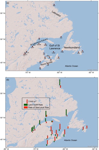
Table 1. Summary of tide-gauge data at 22 stations located along the east coast of Canada.

Station Name	Longitude (°E)	Latitude (°N)	Station ID	Data Period	Years of Data
Argentia	−53.98	47.30	AR	1971–2013	43
Cap-aux-Meules	−61.86	47.38	CAM	1964–2013	18
Charlottetown	−63.12	46.23	CT	1911–2013	92
Halifax	−63.58	44.67	HF	1920–2013	94
Harrington Harbour	−59.48	50.50	HH	1940–1989	47
Lauzon	−71.16	46.83	LZ	1900–2012	100
Lower Escuminac	−64.88	47.08	LE	1973–2013	41
Nain	−61.68	56.55	NN	1964–2013	23
North Sydney	−60.25	46.22	NS	1970–2013	44
Pictou	−62.70	45.68	PT	1957–1995	33
Pointe-au-Père	−68.47	48.52	PAP	1900–1983	72
Port aux Basques	−59.13	47.57	PAB	1936–2013	55
Rimouski-PP^a	−68.51	48.48	RPP	1900–2013	102
Rivière-au-Renard	−64.38	49.00	RAR	1969–2013	44
Saint John	−66.06	45.25	SJ	1905–2013	95
Sainte-Anne-des-Monts	−66.49	49.13	SADM	1969–1997	28
Saint-François IO	−70.81	47.00	SFI	1962–2013	52
Saint-Joseph-de-la-Rive	−70.37	47.45	SJDLR	1969–2013	44
Sept-Îles	−66.38	50.19	SI	1972–2013	42
Shediac Bay	−64.55	46.23	SB	1972–2013	28
St John's	−52.72	47.57	SJS	1936–2013	60
Yarmouth	−66.12	43.83	YM	1900–2013	49

^aRimouski-PP record is a combination of Pointe-au-Père for 1900–1983 and Rimouski for 1984–2013.

The ISDM water level time series at Rimouski from 1984 to 2013 was combined with the time series at Pointe-au-Père from 1900 to 1983 to form a single time series designated Rimouski-PP. At Pointe-au-Père (Rimouski), CD (or the zero of the time series) is 2.588 m (2.583 m) below CGG2010, a recent geoid model produced by Natural Resources Canada (Huang and Véronneau, 2013). If local average surface slopes (which may exist because of local flow dynamics) are ignored and 5 mm is subtracted from the Pointe-au-Père time series, this should reset the zero datum at Pointe-au-Père to that at Rimouski. Assuming this to be the case, the time series have been combined into a record with a duration of more than 100 years.

Prior to extremal analysis, the tide-gauge data were processed as follows: (i) remove non-physical outliers identified as large numbers or by a clear vertical offset, (ii) apply linear detrending to the hourly water levels, (iii) select years that contain at least some data in six of the months, and (iv) compute annual maxima ensuring that any extreme events are separated by at least three days. Between June 1997 and March 2000, there were unresolved technical issues with the tide gauge at Saint John, which caused a lack of confidence in this portion of the time series, so the data for that period were removed prior to carrying out the analysis. In Nain, three peaks during the period between 1980 and 1990 appear to be an error, likely caused by incorrectly applied offsets or instrument disturbances, and this section of data was removed.

Haigh, Nicholls, and Wells (2010) compared the annual maxima method (AMM) and the r-largest method (RLM) for estimating probabilities of extreme water levels. They showed that RLM estimates are larger than AMM estimates at short return periods and are smaller than those of the AMM at long periods. Based on these results, the AMM method was chosen in this study because it provides more conservative estimates of the return levels at long periods and has greater relevance to the design of long-term infrastructure. It is noteworthy that the detrended annual maxima used for the extremal analysis include effects of interannual and decadal variability in mean sea level.

a Rate of Relative Sea-level Rise

The rate of relative SLR at each tide-gauge station is computed using a least-squares fit to annual means of hourly sea-level data for all available years (Table 2). Positive rates mean that relative sea level is rising with respect to land. The standard error in the rate of relative SLR is calculated using the method described in Emery and Thomson (2014). If the autocorrelation of residuals is longer than one year, the effective number of degrees of freedom (N*) is reduced. This is used to adjust the error derived from the least-squares fit and is given by

Table 2. Rate of RSL rise derived from tide-gauge data based on the complete record at each site, and ASL rise derived from tide-gauge and GPS data. Category A represents high-quality level for which t ≥ 50 years and d ≤ 10 km. Category B represents mid-quality level for which 30 ≤ t < 50 years and d ≤ 20 km, and Category C represents low-quality level for usable sites, with 20 ≤ t < 30 years or 20 < d ≤ 40 km. Category F corresponds to unreliable data points for which t < 20 years or d > 40 km.

Names	Rate of SLR (mm yr^−1)		Absolute Sea Level
	Mean	Standard Error	Mean (mm yr^−1)	Standard Error (mm yr^−1)	Category
Argentia	2.3	0.3	1.9	1.1	C
Cap-aux-Meules	4.2	0.3	3.0	0.9	F
Charlottetown	3.3	0.1	2.1	0.8	A
Halifax	3.2	0.1	2.2	0.6	A
Harrington Harbour	−0.7	0.4	−0.8	0.7	F
Lauzon	−0.6	0.3	2.6	0.8	A
Lower Escuminac	3.2	0.5	2.8	0.7	B
Nain	−1.9	0.4	2.6	0.7	C
North Sydney	3.7	0.4	1.9	0.7	F
Pictou	2.2	1.0	0.8	1.2	C
Pointe-au-Père	−0.6	0.4	—	—	—
Port aux Basques	1.6	0.5	1.6	0.8	F
Rimouski-PP	−0.4	0.2	2.8	0.6	A
Rivière-au-Renard	1.1	0.6	2.2	0.8	C
Saint John	2.2	0.2	1.7	0.6	A
Sainte-Anne-des-Monts	−1.2	0.7	1.4	0.9	C
Saint-François IO	0.4	0.8	3.6	1.1	C
Saint-Joseph-de-la-Rive	−1.1	1.3	1.6	1.4	C
Sept-Îles	1.4	0.6	—	—	—
Shediac Bay	3.1	0.5	2.2	0.8	C
St John's	2.2	0.3	2.1	0.6	A
Yarmouth	3.2	0.3	2.0	0.7	B

Here C(τ) is the autocovariance as a function of lag τ, n the number of samples, and Δt the time increment between data values of one year. The maximum number of lag values is based on the significance of the autocorrelation using a p-value (t statistic) less than 0.05. Missing data do not affect the computation of the autocovariance.

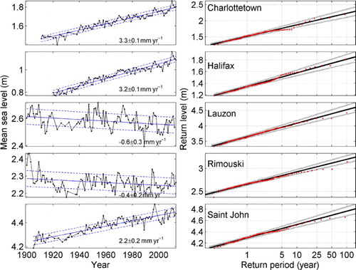
Representative time series of annual means are given for five stations in Fig. 2. The well-defined linear trend (calculated for all available years) is evident although decadal-scale variability leads to different rates of SLR for different periods (Greenberg, Blanchard, Smith, & Barrow, 2012; Hebert, Pettipas, & Petrie, 2012; Han et al., 2014, 2015). In Rimouski, the trend is 1.0 ± 0.4 mm yr⁻¹ between 1984 and 2013 and is −0.4 ± 0.3 mm yr⁻¹ between 1900 and 2013, indicative of the multi-decadal variation in mean sea level. The rates of RSL change show a large-scale spatial structure in Atlantic Canada (Fig. 1b). For the tide gauges with a century-long record in Halifax and Charlottetown, the rate of RSL change is nearly twice as large as the rate of GMSL rise of 1.7 ± 0.2 mm yr⁻¹. The tide-gauge data show a much lower rate of −0.4 ± 0.2 and −0.6 ± 0.3 mm yr⁻¹ in Rimouski-PP and Lauzon, respectively. The rate of 2.2 ± 0.2 mm yr⁻¹ in Saint John is close to the globally averaged rate. Table 2 includes rates of SLR derived for short and long records. Caution is needed in interpreting the rates with shorter records, and they are separated into a different category in Section 5b. Ongoing monitoring and analyses are needed to better understand and correct for interannual variability and to further improve estimates of past SLR in Atlantic Canada, possibly using the approaches presented in White et al. (2014) and Burgette et al. (2013).

Fig. 2 (left) Annual means of hourly water levels for five representative sites. Linear trends were fitted using a least-squares fit. Dashed lines mark the range of two standard deviations. (right) Return level versus return period plots for five representative stations. Solid lines are maximum likelihood curves, and dashed lines show the 95% confidence intervals.

b Statistics of Extreme Water Levels

The detrended annual maxima are fitted to a Gumbel distribution using the “evfit” function of MATLAB^®. The software computes the maximum likelihood estimation of the cumulative density function (1-E) and its 95% confidence intervals. Note that E as used here is the annual exceedance probability (i.e., Eq. (1), with T = 1 year). The fitted curves for each tide-gauge site (Fig. 2) agree reasonably well with the return period based on the ordered annual maxima (marked by the red dots). The return level curves indicate that the 95% confidence interval increases with longer return periods because the data provide less information about higher water levels (Coles, 2001).

The Gumbel model parameters and 50-year return levels for all tide-gauge stations show large spatial variations for Atlantic Canada (Table 3). The location parameter is equal to the 1-year return level and is largely determined by the tides. The smallest location parameter is 0.891 m in Cap-aux-Meules, which is located in the vicinity of an M₂ amphidromic point. The largest value of the location parameter is 4.28 m at Saint John in the Bay of Fundy. The location parameter increases from 2.08 to 4.02 m towards the head of the St. Lawrence Estuary. The scale parameter depends, in a subtle way, on both the distribution of tidal heights and the distribution of surge heights and is represented by the slope of the Gumbel distribution when the height is plotted against the logarithm of the return period. The scale parameter is greater than 0.15 m in the St. Lawrence Estuary and Northumberland Strait where surges are typically largest. The scale parameter is the smallest (∼0.08 m) along the south shore of Newfoundland where tides are relatively small and surges are intermediate (Bernier & Thompson, 2006; Zhang & Sheng, 2013). A smaller-scale parameter indicates that the return period is sensitive to small changes in mean SLR.

Table 3. Statistics of storm tides derived from tide-gauge data. The third, fifth, and seventh columns are the uncertainty estimates (e.g., the location parameter for Argentia is 1.525 ± 0.057, where the error limits are the 2.5 and 97.5 percentiles).

	Location Parameter (m)		Scale Parameter (m)		50-Year Return Level (m)
Station Name	Mean	2.5–97.5 Percentile Range	Mean	2.5–97.5 Percentile Range	Mean	2.5–97.5 Percentile Range
Argentia	1.525	0.057	0.090	0.042	1.877	0.179
Cap-aux-Meules	0.891	0.111	0.114	0.084	1.334	0.365
Charlottetown	1.513	0.067	0.156	0.050	2.121	0.217
Halifax	1.344	0.043	0.101	0.033	1.740	0.144
Harrington Harbour	1.352	0.068	0.113	0.051	1.791	0.225
Lauzon	3.647	0.079	0.190	0.058	4.388	0.256
Lower Escuminac	1.272	0.097	0.149	0.073	1.855	0.321
Nain	1.584	0.094	0.108	0.069	2.007	0.301
North Sydney	1.013	0.073	0.117	0.054	1.469	0.235
Pictou	1.320	0.134	0.185	0.096	2.043	0.412
Pointe-au-Père	2.666	0.060	0.123	0.040	3.148	0.167
Port aux Basques	1.098	0.045	0.080	0.034	1.412	0.146
Rimouski-PP	2.657	0.049	0.118	0.033	3.118	0.139
Rivière-au-Renard	1.403	0.066	0.106	0.051	1.818	0.220
Saint John	4.284	0.046	0.109	0.033	4.709	0.141
Sainte-Anne-des-Monts	2.081	0.088	0.112	0.069	2.520	0.303
Saint-François IO	4.022	0.106	0.185	0.083	4.744	0.365
Saint-Joseph-de-la-Rive	3.594	0.098	0.159	0.077	4.214	0.334
Sept-Îles	2.035	0.086	0.134	0.062	2.558	0.263
Shediac Bay	1.304	0.176	0.225	0.131	2.180	0.575
St John's	1.091	0.043	0.081	0.032	1.406	0.138
Yarmouth	2.609	0.060	0.101	0.045	3.004	0.197

The records of sea-level measurements at tide-gauge stations in Charlottetown, Halifax, Lauzon, Rimouski-PP, and Saint John are longer than 90 years (Table 1). They are used to test how record length and decadal-scale variability affect statistics of extreme water levels. Following Xu, Lefaivre, and Beaulieu (2013), the tide-gauge data are divided into three tri-decade periods, and the extremal analysis is performed for each period. For all locations except Charlottetown the best estimate from the full record falls within the 2.5–97.5 percentile ranges of the estimates from the shorter records (Fig. 3a). For Charlottetown, there is still substantial overlap between the 2.5–97.5 percentile ranges of the full and shorter records.

Fig. 3 (a) Scale parameters and (b) sea-level allowances for RCP8.5_GPS for the 1995–2100 period, estimated from the subsets and full records of detrended annual water level maxima for five tide-gauge stations. The error bars in (a) mark the 2.5–97.5 percentile range.

For long return periods, the return levels are caused by the combined effects of large tides and large surges. The 50-year return level is the largest (>4.7 m) in Saint John and Saint-François IO, where the former has a larger tidal amplitude, and the latter has a larger storm surge. It is the smallest (1.334 m) in Cap-aux-Meules where both tides and surges are small.

4 Projections of relative sea-level rise

A recent report on sea-level allowances for Atlantic Canada (Zhai et al., 2014) used regional projections of the IPCC's AR5 with enhancements to account for GIA and ongoing changes in the Earth's loading and gravitational field. The sea-level projections were fully described in Appendix 1 of Hunter et al. (2013) and were based on the A1FI emission scenario. The allowances presented here are based on the regional projections of RSL change for the IPCC's AR5 RCP8.5 scenario. RCP8.5 is the highest emission scenario in AR5 for the twenty-first century (IPCC, 2013). Recent emissions are tracking closer to RCP8.5 than to other RCPs (Peters et al., 2013).

The regional projections of RSL rise from the AR5 include effects of steric and dynamic changes, atmospheric loading, plus land ice, GIA, and terrestrial water sources (Figs 13.19 and 13.20 in Church et al. (2013)). The steric and dynamic changes are derived from 21 Atmosphere–Ocean General Circulation Models (AOGCMs) from the Coupled Model Intercomparison Project, phase 5 (CMIP5). Following Zhai et al. (2014), the regional sea-level projections from the AR5 were extracted at the locations of 22 tide-gauge stations.

An important difference in the regional projections from Hunter et al. (2013) and AR5 is that uncertainty was estimated for GIA in the latter but not in the former. In AR5 (Church et al., 2013), the GIA contribution was calculated from the mean of the ICE-5G model of the global process of glacial isostatic adjustment (Peltier, 2004) and the Australian National University's (ANU) ice sheet model (Lambeck et al., 1998 and subsequent improvements) with the SEa Level EquatioN (SELEN) solver code for the sea-level equation (Farrell & Clark, 1976; Spada & Stocchi, 2006, 2007), including updates to allow for coastline variation with time, near-field meltwater damping, and Earth rotation in a self-consistent manner (Milne & Mitrovica, 1998; Kendall, Latychev, Mitrovica, Davis, & Tamisiea, 2006). The uncertainties are estimated as half the difference between the two GIA model estimates (Church et al., 2013). There are substantial differences between the GIA estimates in the Atlantic Canada region, so the resultant uncertainties are large, ranging from 0.28 to 4.68 mm yr⁻¹. Rates of RSL change due to GIA in Atlantic Canada (Column 4 of Table 4) shows substantial spatial variations, with rates ranging from −6.16 mm yr⁻¹ in Nain to 0.72 mm yr⁻¹ in North Sydney. Overall, ICE-5G model projections (column 2 of Table 4) are systematically larger than those from the ANU model (column 3 of Table 4).

Table 4. Rates of sea-level change due to the GIA effect estimated from GIA models used for the IPCC's AR5 report.

Names	ICE-5G (mm yr^−1)	ANU (mm yr^−1)	AR5 GIA (mm yr^−1)
			Mean	Standard Error
Argentia	0.21	0.78	0.50	0.28
Cap-aux-Meules	3.05	−2.53	0.26	2.79
Charlottetown	2.35	−1.97	0.19	2.16
Halifax	1.27	−1.04	0.11	1.15
Harrington Harbour	−2.69	−4.15	−3.42	0.73
Lauzon	−1.32	−5.86	−3.59	2.27
Lower Escuminac	2.42	−2.94	−0.26	2.68
Nain	−1.48	−10.84	−6.16	4.68
North Sydney	2.40	−0.96	0.72	1.68
Pictou	2.02	−1.44	0.29	1.73
Pointe-au-Père	−0.01	−5.81	−2.91	2.90
Port aux Basques	1.85	−1.82	0.02	1.83
Rimouski-PP	−0.01	−5.79	−2.90	2.89
Rivière-au-Renard	1.86	−4.12	−1.13	2.99
Saint John	0.74	−2.45	−0.86	1.60
Sainte-Anne-des-Monts	0.65	−5.16	−2.25	2.91
Saint-François IO	−1.16	−5.86	−3.51	2.35
Saint-Joseph-de-la-Rive	−0.97	−6.04	−3.50	2.54
Sept-Îles	−1.58	−6.79	−4.18	2.61
Shediac Bay	1.92	−2.40	−0.24	2.16
St John's	0.27	1.13	0.70	0.43
Yarmouth	0.66	−1.51	−0.42	1.08

Projections of mean RSL change vary from −0.15 m in Nain to 0.83 m in North Sydney between 1995 and 2100 (Zhai et al., 2014). The mean RSL rise is above the global mean in southeast Atlantic Canada. The overall spatial pattern is consistent with that of Han et al. (2014) based on IPCC AR4. Uncertainties in the projected changes in sea level become large towards the end of century (Zhai et al., 2014). For example, the 5th to 95th percentile ranges are −0.99 to 0.69 m at Nain and 0.35 to 1.30 m at North Sydney for 1995–2100.

5 Global positioning system observations

Changes in GPS measurements of height over time indicate the vertical crustal motion relative to the Earth's centre of mass, with positive rates designating land uplift. In Atlantic Canada, the vertical land motion occurs mainly because of GIA (e.g., Koohzare, Vaníček, & Santos, 2008; James et al., 2014). Table 5 (column 2) summarizes the vertical land motion (uplift or subsidence) at tide-gauge stations based on nearby GPS observations. The two primary sources of uncertainty associated with the GPS data are the linear regression error (typically 0.2 mm yr⁻¹) and the uncertainty in the realization of the terrestrial reference frame (about 0.5 mm yr⁻¹; Wu et al., 2011). Analysis of the GPS time series incorporated a coloured noise model to determine rate uncertainties, following the methods described by Mazzotti, Lambert, Henton, James, and Courtier (2011) based on Williams' (2003) formula for a coloured noise source. They are added in quadrature (square root of summed squares) to get the final uncertainty shown in column 3 of Table 5. The GPS data were processed using the Canadian Geodetic Survey's Precise Point Positioning (PPP) software (Kouba & Héroux, 2001). The rates of vertical land motion from PPP were compared with the rates derived from an analysis of the GPS data using the Bernese GPS Software, version 5.0 (Dach et al., 2007), and they are in good agreement. For eastern Canada, GPS estimates of vertical land motion range from 1.13 to 4.56 mm yr⁻¹ of uplift for Quebec to subsidence of up to 1.82 mm yr⁻¹ in Nova Scotia, Prince Edward Island, and southern Newfoundland (James et al., 2014). For Nain, the GPS uplift rate is determined from a Canada-wide GPS velocity field (M. R. Craymer, personal communication, 2011) whose network-adjusted rates have been realigned in a manner consistent with the PPP rates. The uncertainty for Nain is the formal uncertainty of a network adjustment (±0.081 mm yr⁻¹ (M. R. Craymer, personal communication, 2011) and the uncertainty of the reference frame (±0.51 mm yr⁻¹) added in quadrature.

Table 5. Vertical motion derived from GPS data. Corrected GPS rates are used to estimate the adjusted GIA using a linear relationship.

Names	Uplift (mm yr^−1)		Correction^c (mm yr^−1)	Adjusted GIA (mm yr^−1)		Tide-gauge-GPS distance (km)
	Mean^a	Error^b		Mean^d	Error^e
Argentia	−0.40	1.01	−0.29	0.44	1.02	35
Cap-aux-Meules	−1.17	0.80	−0.28	1.13	0.82	161
Charlottetown	−1.17	0.80	−0.28	1.13	0.82	1
Halifax	−1.00	0.55	−0.26	0.96	0.57	3
Harrington Harbour	4.56	0.56	−0.36	−4.04	0.58	492
Lauzon	3.21	0.75	−0.31	−2.85	0.77	8
Lower Escuminac	−0.36	0.55	−0.30	0.41	0.57	6
Nain	4.49	0.58	−0.51	−3.84	0.60	2
North Sydney	−1.82	0.57	−0.28	1.73	0.59	42
Pictou	−1.42	0.61	−0.27	1.35	0.63	22
Pointe-au-Père	3.21	0.56	−0.33	−2.83	0.58	9
Port aux Basques	−0.05	0.61	−0.32	0.14	0.63	176
Rimouski-PP	3.21	0.56	−0.33	−2.83	0.58	4
Rivière-au-Renard	1.13	0.59	−0.33	−0.93	0.61	21
Saint John	−0.52	0.56	−0.27	0.53	0.58	1
Sainte-Anne-des-Monts	2.58	0.56	−0.35	−2.24	0.58	0
Saint-François IO	3.21	0.75	−0.31	−2.85	0.77	38
Saint-Joseph-de-la-Rive	2.68	0.55	−0.32	−2.36	0.57	30
Sept-Îles	4.56	0.56	−0.36	−4.04	0.58	2
Shediac Bay	−0.86	0.58	−0.29	0.86	0.60	1
St John's	−0.13	0.54	−0.29	0.19	0.57	4
Yarmouth	−1.19	0.63	−0.25	1.13	0.65	13

^aUplift rates are relative to the centre of the Earth, as expressed in ITRF2005 (International Terrestrial Reference Frame).

^bUplift error is the square root of summed squares of the linear regression error and the uncertainty of the realization of the terrestrial reference.

^cCorrection is for present-day elastic crustal response to ice-mass changes.

^d<Adjusted GIA mean> = −0.9167 × <Uplift mean + Correction > −0.1947.

^e<Adjusted GIA error> = (<Uplift error>² + <Linear regression error of Fig. 4>²)^1/2.

a Expected Rate of RSL Change Due to GIA

James et al. (2014) showed that GPS rates may be incorporated into sea-level projections and used to derive the rate of RSL change in combination with tide-gauge data. However, it is not as straightforward as simply replacing the modelled GIA rate with the observed GPS rate because of geoid changes associated with GIA. Therefore, an empirical approach has been used to compute the expected rate of RSL change due to GIA (so-called adjusted GIA) as follows:

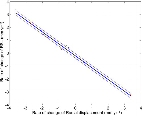
1. For the region of interest (either on a regular grid or at the sites of interest, assuming sufficiently broad distribution), empirically determine the relation between predicted vertical motion and predicted sea-level change for a GIA model or models. The predictions of ICE-5G (VM2 L90), version 1.3 (Peltier, 2004) and ICE-6G (Peltier et al., 2015) were downloaded from http://www.atmosp.physics.utoronto.ca/~peltier/data.php. For 22 tide-gauge sites in Atlantic Canada, the relationship between the predicted vertical uplift rate and rate of RSL change was found to be linear (Fig. 4). The slope of the line is −0.9167, indicating that the geoid rates are about 10% of the uplift rates and that they act in the opposite sense of the vertical deformation for controlling relative sea level. The intercept (on the vertical axis) of −0.1947 is related to the increasing size of the global basins due to GIA (Peltier, 2009; Church et al., 2013). The regression, based on the combined ICE-5G/6G predictions represents current knowledge and understanding of the GIA process in North America, is constrained by several geodetic and geological observables, and incorporates uncertainties in the ice-load history.

   Fig. 4 Relationship between predicted vertical uplift rate and rate of RSL change for the ICE-5G (VM2) model, version 1.3 (Peltier, 2004) and ICE-6G (Peltier et al., 2015) indicated by red dots. The solid blue line is the regression: < Rate of relative sea-level change >  = –0.9167 < vertical uplift > –0.1947. The dashed lines mark the range of two standard deviations of the error.

   

2. Correct GPS vertical rates for the (relatively small) elastic effect due to present ice-mass changes following James et al. (2014). The elastic correction term (column 4 of Table 5) is about −0.3 mm yr⁻¹ for present-day ice-mass change. The correction is required to isolate the portion of the GPS uplift signal due to the GIA.

3. Apply the linear relation from step 1 to the corrected GPS rates to obtain the ongoing sea-level change resulting from vertical crustal motion (henceforth termed “adjusted GIA” in contrast to the modelled GIA).

4. This conversion is appropriate for Atlantic Canada because the GPS vertical rate is due mainly to the GIA effect (Koohzare et al., 2008). The purpose of steps 1–3 in this process is to replace the modelled GIA with the adjusted GIA. The uncertainty from the linear regression of step 1 is added in quadrature to the GPS uncertainty to calculate the error of the adjusted GIA.

b Comparison with Tide-gauge Data

An analysis that was carried out by Mazzotti, Jones, and Thomson (2008) for the Pacific coast of Canada was replicated to show the consistency between tide-gauge records and GPS measurements by comparing tide-gauge trends to GPS uplift rates. The data were divided into four categories (A, B, C, and F) based on the length of the tide-gauge record (t) and the distance (d) between tide-gauge and GPS sites following Mazzotti et al. (2008). Category A represents high-quality data for which t ≥ 50 years and d ≤ 10 km. Category B represents mid-quality data for which 30 ≤ t < 50 years and  d ≤ 20 km, and Category C represents low-quality data for usable sites, with 20 ≤ t < 30 years or 20 < d ≤ 40 km. Category F corresponds to unreliable data points for which t < 20 years or d > 40 km.

The rate of RSL change derived from tide-gauge data versus the GPS uplift rate for the Category A, B, and C sites (Table 2) is given in Fig. 5a. The line was constrained to a slope of −1. The y-intercept of the line is the average of the tide-gauge rate minus the GPS rate (the Sept-Îles and Pointe-au-Père tide gauges were removed, as explained in the following). The intercept represents the rate of RSL change for a situation in which the vertical land motion is zero and corresponds to the absolute sea-level (ASL) rise, which is SLR relative to the centre of mass or geocentre of the Earth. For Atlantic Canada, the ASL rise is 2.2 ± 0.2 mm yr⁻¹ with a scatter around the mean (standard deviation) of 0.7 mm yr⁻¹. The range of uncertainty for the ASL rate encompasses the GMSL rise of 1.7 ± 0.2 mm yr⁻¹ since 1900 (Church et al., 2013). The difference between local ASL rise and the global average is 0.5 ± 0.3 mm yr⁻¹, indicating consistency of the GPS and tide-gauge trends in the region and that GIA explains the overall spatial pattern of tide-gauge trends in Atlantic Canada.

Fig. 5 (a) The rate of RSL change (mm yr⁻¹) derived from tide-gauge data versus the adjusted GIA rate based on GPS observations. The solid line was constrained to a slope of −1. (b) Modelled GIA rate (based on the average of ICE-5G and ANU models (Church et al., 2013)) versus adjusted GIA rate based on GPS observations. The solid blue line is the regression: <Adjusted GIA rate> = 0.96 < Modelled GIA rate> + 0.57. The error bars in the y-direction mark the two standard deviation range. The error bars in the x-direction mark the absolute difference of the two GIA models.

The point corresponding to the Pointe-au-Père tide gauge was removed to avoid overweighting SLR at Rimouski. The tide-gauge rate minus the RSL rate due to GIA at Sept-Îles is high (5.4 ± 1.0 mm yr⁻¹) and is likely affected by the decadal variations in river runoff and atmospheric forcing from 1972 to 2013. A longer record of tide-gauge measurements or removal of natural fluctuations may be needed for a robust detection of sea-level change at Sept-Îles.

The rate of ASL rise for all tide gauges in Atlantic Canada was tested for its sensitivity to the joint quality level of both tide-gauge and GPS measurements. Figure 5a shows sites with three quality levels. The ASL rate is 2.3 ± 0.3 mm yr⁻¹ for Category A, 2.4 ± 0.4 mm yr⁻¹ for Category B, and 2.0 ± 0.4 mm yr⁻¹ for Category C, indicating relative consistency among the different quality levels and the overall dataset.

c Comparison with the Projected Rate of RSL Change Due to GIA

The adjusted GIA data are compared with the GIA model predictions (Fig. 5b) used for the RSL projections of the IPCC AR5 (Church et al., 2013). The root-mean-square errors of the ICE-5G model, ANU model, and their average (relative to the adjusted GIA rates) are 1.75, 3.08, and 0.93 mm yr⁻¹, respectively. The y-intercept of the regression line indicates an offset, or bias, between the model predictions and the GPS observations. The biases for the ICE-5G model, ANU model, and their average are –1.47, 1.27, and 0.57 mm yr⁻¹, respectively, and this bias would amount to −15, 13, and 6.0 cm over 105 years (1995–2100). This shows that the average of two GIA models is relatively well explained by the adjusted GIA rates (Fig. 5b). The difference between the two GIA model predictions are large and generate large uncertainties, with a median of 2.2 mm yr⁻¹ and a 5th to 95th percentile range of 0.4–3.7 mm yr⁻¹. In comparison, the uncertainties in the adjusted GIA rates are much smaller and generally range between 0.6 and 1.0 mm yr⁻¹ (5th to 95th percentile range).

6 Regional sea-level allowances

The sea-level allowances for 22 tide-gauge sites were calculated using the regional sea-level projections of RCP8.5 from AR5 (Tables 6 and 7; Fig. 6) and then re-calculated using the same projections except that the modelled GIA portion is replaced with the adjusted GIA (Tables 8 and 9; Fig. 6). There are, therefore, two groups of allowances:

1. Sea-level allowances based on the regional RCP8.5 sea-level projections from AR5.

   Fig. 6 Sea-level allowances at tide-gauge stations along the Atlantic coast of Canada (a) for the 1995–2050 period and (b) for the 1995–2100 period. Green vertical bars show the sea-level allowances for RCP8.5, and the red vertical bars show the sea-level allowances for which the modelled GIA projections are replaced by the adjusted GIA projections based on GPS uplift rates. The scale of the red vertical bar in the legend is 0.5 m.

   

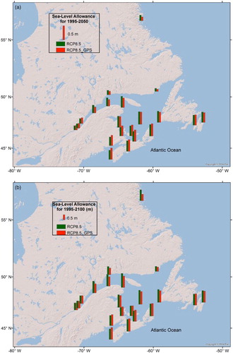
   Table 6. Summary of projected sea-level change and sea-level allowances for RCP8.5 and 1995–2050 at tide-gauge stations along the Atlantic coast of Canada. SLR projections are based on IPCC AR5.

   Station Name	Scale Parameter (m)	RCP8.5 Projection (m)				Allowance (m)
   		Mean	Standard Deviation	5th Percentile	95th Percentile
   Argentia	0.090	0.32	0.08	0.19	0.45	0.36
   Cap-aux-Meules	0.114	0.31	0.18	0.02	0.60	0.45
   Charlottetown	0.156	0.28	0.15	0.03	0.54	0.36
   Halifax	0.101	0.32	0.11	0.14	0.50	0.38
   Harrington Harbour	0.113	0.08	0.09	−0.07	0.22	0.11
   Lauzon	0.190	0.10	0.14	−0.14	0.34	0.15
   Lower Escuminac	0.149	0.28	0.18	−0.02	0.58	0.40
   Nain	0.108	−0.12	0.26	−0.55	0.31	0.20
   North Sydney	0.117	0.34	0.13	0.13	0.55	0.41
   Pictou	0.185	0.31	0.14	0.09	0.54	0.36
   Pointe-au-Père	0.123	0.12	0.18	−0.18	0.42	0.25
   Port aux Basques	0.080	0.30	0.13	0.08	0.51	0.40
   Rimouski-PP	0.118	0.12	0.18	−0.18	0.42	0.26
   Rivière-au-Renard	0.106	0.23	0.19	−0.08	0.54	0.40
   Saint John	0.109	0.24	0.12	0.05	0.44	0.31
   Sainte-Anne-des-Monts	0.112	0.15	0.18	−0.15	0.46	0.30
   Saint-François IO	0.185	0.10	0.15	−0.14	0.34	0.16
   Saint-Joseph-de-la-Rive	0.159	0.10	0.15	−0.15	0.36	0.18
   Sept-Îles	0.134	0.05	0.18	−0.24	0.34	0.16
   Shediac Bay	0.225	0.26	0.15	0.01	0.51	0.31
   St John's	0.081	0.33	0.08	0.19	0.47	0.37
   Yarmouth	0.101	0.27	0.11	0.10	0.45	0.33

   Table 7. Summary of projected sea-level change and sea-level allowances for RCP8.5 and 1995–2100 at tide-gauge stations along the Atlantic coast of Canada. SLR projections are based on IPCC AR5.

   Station Name	Scale Parameter (m)	RCP8.5 Projection (m)				Allowance (m)
   		Mean	Standard Deviation	5th Percentile	95th Percentile
   Argentia	0.090	0.80	0.22	0.43	1.16	1.07
   Cap-aux-Meules	0.114	0.76	0.37	0.16	1.37	1.36
   Charlottetown	0.156	0.68	0.30	0.18	1.18	0.98
   Halifax	0.101	0.84	0.26	0.41	1.27	1.17
   Harrington Harbour	0.113	0.29	0.21	−0.06	0.64	0.49
   Lauzon	0.190	0.42	0.32	−0.10	0.95	0.68
   Lower Escuminac	0.149	0.73	0.39	0.10	1.37	1.23
   Nain	0.108	−0.15	0.51	−0.99	0.69	1.06
   North Sydney	0.117	0.83	0.29	0.35	1.30	1.19
   Pictou	0.185	0.78	0.31	0.27	1.28	1.03
   Pointe-au-Père	0.123	0.43	0.38	−0.19	1.06	1.02
   Port aux Basques	0.080	0.74	0.29	0.27	1.21	1.25
   Rimouski-PP	0.118	0.44	0.38	−0.19	1.06	1.05
   Rivière-au-Renard	0.106	0.62	0.40	−0.03	1.27	1.36
   Saint John	0.109	0.66	0.27	0.22	1.10	0.99
   Sainte-Anne-des-Monts	0.112	0.50	0.38	−0.12	1.13	1.15
   Saint-François IO	0.185	0.43	0.32	−0.10	0.96	0.71
   Saint-Joseph-de-la-Rive	0.159	0.43	0.33	−0.11	0.98	0.77
   Sept-Îles	0.134	0.30	0.37	−0.30	0.90	0.80
   Shediac Bay	0.225	0.64	0.30	0.14	1.14	0.84
   St John's	0.081	0.83	0.23	0.45	1.20	1.14
   Yarmouth	0.101	0.72	0.25	0.31	1.13	1.03

   Table 8. Summary of projected sea-level change and sea-level allowances for RCP8.5_GPS and 1995–2050 at tide-gauge stations along the Atlantic coast of Canada. GIA model projections of IPCC AR5 are replaced with the adjusted GIA data derived from GPS uplift rates.

   Station Name	Scale Parameter (m)	RCP8.5_GPS Projection (m)				Allowance (m)
   		Mean	Standard Deviation	5th Percentile	95th Percentile
   Argentia	0.090	0.32	0.09	0.17	0.47	0.37
   Cap-aux-Meules	0.114	0.36	0.13	0.14	0.58	0.44
   Charlottetown	0.156	0.34	0.13	0.13	0.54	0.39
   Halifax	0.101	0.37	0.10	0.20	0.53	0.42
   Harrington Harbour	0.113	0.04	0.09	−0.10	0.19	0.08
   Lauzon	0.190	0.14	0.11	−0.04	0.32	0.17
   Lower Escuminac	0.149	0.32	0.14	0.08	0.56	0.39
   Nain	0.108	0.01	0.17	−0.27	0.28	0.14
   North Sydney	0.117	0.39	0.11	0.22	0.57	0.44
   Pictou	0.185	0.37	0.12	0.17	0.56	0.41
   Pointe-au-Père	0.123	0.12	0.14	−0.10	0.35	0.20
   Port aux Basques	0.080	0.30	0.11	0.12	0.48	0.37
   Rimouski-PP	0.118	0.12	0.14	−0.10	0.35	0.20
   Rivière-au-Renard	0.106	0.24	0.14	0.01	0.47	0.34
   Saint John	0.109	0.32	0.10	0.16	0.49	0.37
   Sainte-Anne-des-Monts	0.112	0.16	0.14	−0.07	0.38	0.24
   Saint-François IO	0.185	0.14	0.11	−0.04	0.32	0.17
   Saint-Joseph-de-la-Rive	0.159	0.17	0.11	−0.01	0.35	0.21
   Sept-Îles	0.134	0.06	0.14	−0.17	0.28	0.13
   Shediac Bay	0.225	0.32	0.12	0.12	0.52	0.36
   St John's	0.081	0.30	0.09	0.16	0.44	0.35
   Yarmouth	0.101	0.36	0.10	0.20	0.52	0.41

   Table 9. Summary of projected sea-level change and sea-level allowances for RCP8.5_GPS and 1995–2100 at tide-gauge stations along the Atlantic coast of Canada. GIA model projections from IPCC AR5 are replaced with the adjusted GIA data derived from GPS uplift rates.

   Station Name	Scale Parameter (m)	RCP8.5_GPS Projection (m)				Allowance (m)
   		Mean	Standard Deviation	5th Percentile	95th Percentile
   Argentia	0.090	0.79	0.24	0.40	1.18	1.10
   Cap-aux-Meules	0.114	0.85	0.30	0.37	1.34	1.24
   Charlottetown	0.156	0.78	0.26	0.36	1.20	0.99
   Halifax	0.101	0.93	0.25	0.52	1.34	1.23
   Harrington Harbour	0.113	0.23	0.21	−0.13	0.57	0.42
   Lauzon	0.190	0.50	0.27	0.07	0.94	0.68
   Lower Escuminac	0.149	0.80	0.32	0.28	1.33	1.15
   Nain	0.108	0.09	0.34	−0.47	0.66	0.64
   North Sydney	0.117	0.93	0.26	0.51	1.36	1.22
   Pictou	0.185	0.89	0.28	0.43	1.35	1.10
   Pointe-au-Père	0.123	0.44	0.30	−0.05	0.94	0.81
   Port aux Basques	0.080	0.75	0.25	0.34	1.16	1.14
   Rimouski-PP	0.118	0.44	0.30	−0.05	0.94	0.83
   Rivière-au-Renard	0.106	0.64	0.31	0.12	1.16	1.11
   Saint John	0.109	0.80	0.24	0.41	1.20	1.07
   Sainte-Anne-des-Monts	0.112	0.51	0.30	0.01	1.00	0.91
   Saint-François IO	0.185	0.50	0.27	0.07	0.94	0.69
   Saint-Joseph-de-la-Rive	0.159	0.55	0.26	0.12	0.99	0.77
   Sept-Îles	0.134	0.32	0.30	−0.18	0.81	0.65
   Shediac Bay	0.225	0.75	0.25	0.34	1.17	0.89
   St John's	0.081	0.77	0.23	0.40	1.15	1.10
   Yarmouth	0.101	0.88	0.24	0.49	1.28	1.16

2. Sea-level allowances based on the regional RCP8.5 sea-level projections of AR5 for which the modelled GIA is replaced with the adjusted GIA estimated from GPS data, referred to here as the RCP8.5_GPS.

The median, 5th, and 95th percentiles of the difference between sea-level allowances for RCP8.5 and RCP8.5_GPS are 0, −0.07, and 0.07 m, respectively, for the 1995–2050 period (Fig. 6a, Table 8) and 0.04, −0.10, and 0.33 m, respectively, for the 1995–2100 period (Fig. 6b, Table 9). The reduced uncertainty in sea-level projections for RCP8.5_GPS reduces the allowances in Nain and the St. Lawrence Estuary. The sea-level allowances for RCP8.5_GPS (Fig. 6; Tables 7 and 9) are slightly larger than those for RCP8.5 along the coasts of Nova Scotia, Prince Edward Island, and the Gulf of Maine, a consequence of the small underestimation of the means of GIA model predictions. Incorporating GPS rates results in an increase of a few centimetres in sea-level allowances for the coasts of Nova Scotia and Prince Edward Island but results in a decrease of several tens of centimetres in Nain and the St. Lawrence Estuary for 1995–2100.

The allowance is composed of two parts: the mean SLR (Δz) and the term arising from the uncertainty in future SLR. For the 1995–2050 period, the allowances (Tables 6 and 8) lie between the mean projections and the mean plus one standard deviation. For comparison, Tables 7 and 9 show that the allowances for the 1995–2100 period are closer to the 95th percentile of the projections at most sites. But for stations in Northumberland Strait and the head of the St. Lawrence Estuary, sea-level allowances for 1995–2100 are less than the mean plus one standard deviation of SLR because of the large-scale parameters in those regions. The increase in the difference between the allowance and the mean projection with time is related to the increasing uncertainty of sea-level projections with time and the fact that the allowance depends on the square of the uncertainty.

Sea-level allowances at 22 tide gauges (Fig. 6) show a significant spatial variation, largely affected by spatially varying projections of SLR. For RCP8.5_GPS, the range of allowances is 0.08 m to 0.44 m for the 1995–2050 period (Table 8) and 0.42 to 1.24 m for the 1995–2100 period (Table 9). Where the land is sinking, the allowances for 2100 are largest and reach more than 1 m in Nova Scotia, the Bay of Fundy, Prince Edward Island, and southern Newfoundland (Fig. 6b). Where the land is rising quickly, the allowances for 2100 are as small as 0.42 m in Harrington Harbour (Fig. 6b). The allowances are tested for the uncertainties on scale parameters derived from the sub-sampled records at five tide-gauge stations. Figure 3b shows that the allowances based on scale parameters estimated from the sub-sampled records only differ by −3 to 9 cm from the allowances based on scale parameters estimated from their full records for RCP8.5_GPS and for 2100.

7 Conclusions

This paper provides the scientific basis and the methodology for deriving sea-level allowances for Atlantic Canada using the AR5 projections and incorporating GPS measurements of vertical land motion. The tide-gauge data have been analyzed to determine the presentage trend of RSL change and the statistics of storm tides. The GPS rates were introduced to compute the expected rates of sea-level change due to vertical land motion, which were used to derive the rate of ASL rise for Atlantic Canada. The GIA model rates differ from the GPS rates, and it is suggested that allowances based on measured GPS rates be adopted.

In most regions of Atlantic Canada, new infrastructure will need to be built higher off the ground to account for future SLR. This allowance depends only on the projected rise in mean sea level and its uncertainty and on the scale parameter of a Gumbel distribution derived from tide-gauge records. The allowances show large spatial variations, a consequence of using spatially varying projected RSL change and storm-tide statistics. In the Bay of Fundy and Gulf of Maine, the sea-level allowances should take account of the change in tidal amplitude because SLR will induce an expanded tidal range over the twenty-first century in this region (Greenberg et al., 2012).

The IPCC AR5 indicates that instability of the western Antarctic ice sheet could contribute additional tens of centimetres of global SLR by 2100 although the contribution is poorly constrained (Church et al., 2013; James et al., 2014). In research published after the release of the IPCC's AR5 (or RCP8.5, the IPCC AR5 sea-level rise by 2100 is 0.52 to 0.98 m relative to 1986–2005 (Church et al., 2013)), an expert assessment of SLR reported that the likely ranges are 0.7–1.2 m by 2100 and 2–3 m by 2300 for the high-emissions RCP8.5 scenario (Horton, Rahmstorf, Engelhart, & Kemp, 2014). Joughin, Smith, and Medley (2014) show that the collapse of the western Antarctic ice sheet is starting and that its meltwater would raise sea levels by more than 3 m over several centuries. Kopp et al. (2014) projected a very likely (90% probability) GMSL rise of 0.5 to 1.2 m under RCP8.5 between 2000 and 2100. Talke, Orton, and Jay (2014) suggest that annual maximum storm tides in New York Harbor contain both multi-decadal variability and a secular trend in each quartile. Collectively, these recent studies may indicate that the estimates of sea-level allowances based on the IPCC's AR5 report are conservative (e.g., Hinkel et al., 2015). Nevertheless, the GPS-based allowances described here may be useful for planning purposes because they are based on direct measurements of vertical land motion and were derived from rigorous combination of storm-surge recurrence with the largest likely projections of the IPCC AR5.

Acknowledgements

We thank Mark Carson from the Institut für Meereskunde, Universität Hamburg for producing and providing the IPCC's AR5 projections, John Loder, Brian Petrie, Joel Chassé, and Zeliang Wang for their constructive discussions, and Zeliang Wang and Shannon Nudds for internal reviews.

Disclosure statement

No potential conflict of interest was reported by the authors.

Funding

This work is funded by the DFO Aquatic Climate Change Adaptation Services Program (ACCASP). This is an output of the NRCan Climate Change Geoscience Program. Support from the NRCan Climate Change Impacts and Adaptation Division is gratefully acknowledged by T.S. James. This is Earth Sciences Sector, Natural Resources Canada, contribution number [20140459].

References

- Aerts, J. C. J. H., Botzen, W. J. W., Emanuel, K., Lin, N., de Moel, H., & Michel-Kerjan, E. O. (2014). Evaluating flood resilience strategies for coastal megacities. Science, 344(6183), 473–475. doi:10.1126/science.1248222
- Bernier, N. B., & Thompson, K. R. (2006). Predicting the frequency of storm surges and extreme sea levels in the northwest Atlantic. Journal of Geophysical Research, 111, C10009, 1–15. doi:10.1029/2005JC003168
- Burgette, R. J., Watson, C. S., White, N. J., Church, J. A., Tregoning, P., & Coleman, R. (2013). Characterizing and minimizing the effects of noise in tide gauge time series: Relative and geocentric sea level rise around Australia. Geophysical Journal International, 194(2), 719–736. doi: 10.1093/gji/ggt131
- Church, J. A., Clark, P. U., Cazenave, A., Gregory, J. M., Jevrejeva, S., Levermann, A., … Unnikrishnan A. S. (2013). Sea level change. pp. 1139–1216. In T. F. Stocker, D. Qin, G.-K. Plattner, M. Tignor, S. K. Allen, J. Boschung, A. Nauels, Y. Xia, V. Bex, & P. M. Midgley (Eds.), Climate change 2013: The physical science basis. Contribution of Working Group I to the Fifth Assessment Report of the Intergovernmental Panel on Climate Change. Cambridge, United Kingdom and New York, NY, USA: Cambridge University Press.
- Coles, S. (2001). An introduction to statistical modeling of extreme values. London, Berlin, Heidelberg: Springer-Verlag.
- Dach, R., Beutler, G., Bock, H., Fridez, P., Gäde, A., Hugentobler, U., … Walser, P. (2007). Bernese GPS Software Version 5.0. Astronomical Institute, University of Bern, Bern, Switzerland. Retrieved from ftp://ftp.space.dtu.dk/pub/fch/bernese/DOCU50.pdf
- Emery, W. J., & Thomson, R. E. (2014). Data analysis methods in physical oceanography, 3rd edition, Section 3.15.2, William J. Emery and Richard E. Thomson (Eds.), Elsevier Science, Amsterdam, ISBN 9780123877826.
- Farrell, W. E., & Clark, J. A. (1976). On postglacial sea-level. Geophysical Journal of the Royal Astronomical Society, 46, 647–667. doi: 10.1111/j.1365-246X.1976.tb01252.x
- Greenberg, D. A., Blanchard, W., Smith, B., & Barrow, E. (2012). Climate change, mean sea level and high tides in the Bay of Fundy. Atmosphere-Ocean, 50, 261–276. doi:10.1080/07055900.2012.668670
- Guo, L., Perrie, W., Long, Z., Chassé, J., Zhang, Y., & Huang, A. (2013). Dynamical downscaling over the Gulf of St. lawrence using the Canadian Regional Climate Model. Atmosphere-Ocean, 51(3), 265–283. doi:10.1080/07055900.2013.798778
- Haigh, I., Nicholls, R., & Wells, N. (2010). A comparison of the main methods for estimating probabilities of extreme still water levels. Coastal Engineering, 57, 838–849. doi: 10.1016/j.coastaleng.2010.04.002
- Han, G., Ma, Z., Bao, H., & Slangen, A. (2014). Regional differences of relative sea level changes in the Northwest Atlantic: Historical trends and future projections. Journal of Geophysical Research: Oceans, 119, 156–164. doi:10.1002/2013JC009454
- Han, G., Ma, Z., Chen, N., Thomson, R., & Slangen, A. (2015). Changes of mean relative sea level around Canada in the 20th and 21st centuries. Atmosphere-Ocean, 53, 1–12. doi:10.1080/07055900.2015.1057100
- Hebert, D., Pettipas, R., & Petrie, B. (2012). Meteorological, sea ice and physical oceanographic conditions on the Scotian Shelf and in the Gulf of Maine during 2011. DFO Can. Sci. Advis. Sec. Res. Doc. 2012/055. Ottawa, Ontario: Fisheries and Oceans Canada.
- Hinkel, J., Jaeger, C., Nicholls, R. J., Lowe, J., Renn, O., & Peijun, S. (2015). Sea-level rise scenarios and coastal risk management. Nature Climate Change., 5, 188–190. doi: 10.1038/nclimate2505
- Hinkel, J., Lincke, D., Vafeidis, A. T., Perrette, M., Nicholls, R. J., Tol, R. S. J., … Levermann, A. (2014). Coastal flood damage and adaptation costs under 21st century sea-level rise. Proceedings of the National Academy of Sciences, 111, 3292–3297. doi:10.1073/pnas.1222469111
- Horton, B. P., Rahmstorf, S., Engelhart, S. E., & Kemp, A. C. (2014). Expert assessment of sea-level rise by AD 2100 and AD 2300. Quaternary Science Reviews, 84, 1–6. doi:10.1016/j.quascirev.2013.11.002
- Huang, J., & Véronneau, M. (2013). Canadian gravimetric geoid model 2010. Journal of Geodesy, 87, 771–790. doi:10.1007/s00190-013-0645-0
- Hunter, J. (2012). A simple technique for estimating an allowance for uncertain sea-level rise. Climatic Change, 113, 239–252. doi:10.1007/s10584–011-0332-1
- Hunter, J., Church, J. A., White, N. J., & Zhang, X. (2013). Towards a global regionally-varying allowance for sea-level rise. Ocean Engineering, 71, 17–27. doi:10.1016/j.oceaneng.2012.12.041
- IPCC. (2013). Annex III: Glossary [Planton, S. (Ed.)]. In T. F. Stocker, D. Qin, G.-K. Plattner, M. Tignor, S. K. Allen, J. Boschung, A. Nauels, Y. Xia, V. Bex, & P. M. Midgley (Eds.), Climate Change 2013: The Physical Science Basis. Contribution of Working Group I to the Fifth Assessment Report of the Intergovernmental Panel on Climate Change. Cambridge, United Kingdom and New York, NY, USA: Cambridge University Press.
- James, T. S., Henton, J. A., Leonard, L. J., Darlington, A., Forbes, D. L., & Craymer, M. (2014). Relative sea-level projections in Canada and the adjacent mainland United States. Geological Survey of Canada, Open File 7737, doi:10.4095/295574. Retrieved from http://wmsmir.cits.rncan.gc.ca/index.html/pub/geott/ess_pubs/295/295574/of_7737.pdf
- James, T. S., & Morgan, W. J. (1990). Horizontal motions due to post-glacial rebound. Geophysical Research Letters., 17, 957–960. doi: 10.1029/GL017i007p00957
- Joughin, I., Smith, B. E., & Medley, B. (2014). Marine ice sheet collapse potentially underway for the Thwaites Glacier Basin, West Antarctica. Science, 344(6185), 735–738. doi: 10.1126/science.1249055
- Kendall, R., Latychev, K., Mitrovica, J. X., Davis, J. E., & Tamisiea, M. (2006). Decontaminating tide gauge records for the influence of Glacial Isostatic Adjustment: The potential impact of 3-D Earth structure. Geophysical Research Letters., 33, L24318, 1–5. doi:10.1029/2006GL028448
- Koohzare, A., Vaníček, P., & Santos, M. (2008). Pattern of recent vertical crustal movements in Canada. Journal of Geodynamics, 45, 133–145. doi: 10.1016/j.jog.2007.08.001
- Kopp, R. E., Horton, R. M., Little, C. M., Mitrovica, J. X., Oppenheimer, M., Rasmussen, D. J., … Tebaldi, C. (2014). Probabilistic 21st and 22nd century sea-level projections at a global network of tide gauge sites. Earth's Future, 2, 383–406. doi:10.1002/2014EF000239
- Kouba, J., & Héroux, P. (2001). Precise point positioning using IGS orbit and clock products. GPS Solutions., 5(2), 12–28. doi: 10.1007/PL00012883
- Lambeck, K., Smither, C., & Ekman, M. (1998). Tests of glacial rebound models for Fennoscandinavia based on instrumented sea- and lake-level records. Geophysical Journal International., 135, 375–387. doi: 10.1046/j.1365-246X.1998.00643.x
- Mazzotti, S., Jones, C., & Thomson, R. E. (2008). Relative and absolute sea level rise in western Canada and northwestern United States from a combined tide gauge-GPS analysis. Journal of Geophysical Research, 113, C11019, 1–19. doi:10.1029/2008JC004835
- Mazzotti, S., Lambert, A., Henton, J., James, T. S., & Courtier, N. (2011). Absolute gravity calibration of GPS velocities and glacial isostatic adjustment in mid-continent North America. Geophysical Research Letters, 38, L24311, 1–5. doi:10.1029/2011GL049846
- Milne, G. A., & Mitrovica, J. X. (1998). Postglacial sea-level change on a rotating Earth. Geophysical Journal International, 133, 1–19. doi: 10.1046/j.1365-246X.1998.1331455.x
- Peltier, W. (2004). Global glacial isostasy and the surface of the ice-age earth: The ICE-5G (VM2) model and GRACE. Annual Review of Earth and Planetary Sciences, 32, 111–149. doi: 10.1146/annurev.earth.32.082503.144359
- Peltier, W. R. (2009). Closure of the budget of global sea level rise over the GRACE era: The importance and magnitudes of the required corrections for global glacial isostatic adjustment. Quaternary Science Reviews., 28, 1658–1674. doi: 10.1016/j.quascirev.2009.04.004
- Peltier, W. R., Argus, D. F., & Drummond, R. (2015). Space geodesy constrains ice-age terminal deglaciation: The global ICE-6G_C (VM5a) model. Journal of Geophysical Research Solid Earth, 120, 450–487. doi:10.1002/2014JB011176
- Peters, G. P., Andrew, R. M., Boden, T., Canadell, J. G., Ciais, P., Le Quéré, C., … Wilson, C. (2013). The challenge to keep global warming below 2 °C, Nature Climate. Change, 3, 4–6. doi:10.1038/nclimate1783
- Pugh, D. (1996). Tides, surges and mean sea-level. John Wiley & Sons, reprinted with corrections. Chichester, New York, Brisbane, Toronto and Singapore. Retrieved from http://core.ac.uk/download/pdf/31990.pdf
- Ranasinghe, R., Duong, T. M., Uhlenbrook, S., Roelvink, D., & Stive, M. (2012). Climate-change impact assessment for inlet-interrupted coastlines. Nature, 3, 83–87. doi:10.1038/nclimate1664
- Shepherd, T. G. (2014). Atmospheric circulation as a source of uncertainty in climate change projections. Nature Geoscience., 7, 703–708. doi:10.1038/NGEO2253
- Spada, G., & Stocchi, P. (2006). The sea level equation, theory and numerical examples. Rome: Aracne, ISBN: 88–548-0384-7.
- Spada, G., & Stocchi, P. (2007). SELEN: A Fortran 90 program for solving the “sea level equation”. Computers & Geosciences., 33(4), 538–562. doi:10.1016/j.cageo.2006.08.006
- Talke, S. A., Orton, P., & Jay, D. A. (2014). Increasing storm tides in New York Harbor, 1844–2013. Geophysical Research Letters, 41, 3149–3155. doi:10.1002/2014GL059574
- Walcott, R. I. (1972). Late Quaternary vertical movements in eastern North America: Quantitative evidence of glacio-isostatic rebound. Reviews of Geophysics and Space Physics, 10, 849–884. doi: 10.1029/RG010i004p00849
- White, N. J., Haigh, I. D., Church, J. A., Koen, T., Watson, C. S., Pritchard, T. R., … Tregoning, P. (2014). Australian sea levels trends, regional variability and influencing factors. Earth-Science Reviews, 136, 155–174. doi: 10.1016/j.earscirev.2014.05.011
- Williams, S. D. P. (2003). The effect of colored noise on the uncertainties of rates estimated from geodetic series. Journal of Geodesy, 76, 483–494. doi:10.1007/s00190-002-0283-4
- Wu, X., Collilieux, X., Altamimi, Z., Vermeersen, B. L. A., Gross, R. S., & Fukumori, I. (2011). Accuracy of the International Terrestrial Reference Frame origin and Earth expansion. Geophysical Research Letters, 38, L13304, 1–5. doi:10.1029/2011GL047450
- Xu, Z., Lefaivre, D., & Beaulieu, M. (2013). Sea levels and storm surges in the Gulf of St. Lawrence and its vicinity. Ch.8 (p. 95–112). In J. W. Loder, G. Han, P. S. Galbraith, J. Chassé, & A. van der Baaren (Eds.), Aspects of climate change in the Northwest Atlantic off Canada. Can. Tech. Rep. Fish. Aquat. Sci.
- Zhai, L., Greenan, B., Hunter, J., Han, G., Thomson, R., & MacAulay, P. (2014). Estimating sea-level allowances for the coasts of Canada and the adjacent United States using the Fifth Assessment Report of the IPCC. Can. Tech. Rep. Hydrogr. Ocean. Sci. 300. Retrieved from http://publications.gc.ca/site/eng/472837/publication.html
- Zhai, L., Greenan, B., Hunter, J., James, T. S., & Han, G. (2013). Estimating sea-level allowances for Atlantic Canada under conditions of uncertain sea-level rise. Can. Tech. Rep. Hydrogr. Ocean. Sci. 283. Retrieved from http://publications.gc.ca/site/eng/455019/publication.html
- Zhang, H., & Sheng, J. (2013). Estimation of extreme sea levels over the eastern continental shelf of North America. Journal of Geophysical Research: Oceans, 118, 6253–6273. doi:10.1002/2013JC009160