Static Stability of the Troposphere Over the Southeastern Beaufort Sea–Amundsen Gulf Region of the Western Maritime Arctic

Abstract

The characterization of the static stability of the troposphere over the western maritime Arctic remains limited in spite of its significance to both atmospheric thermodynamics and dynamics. Field observations of microwave radiometric temperature profiles from the International Polar Year, Circumpolar Flaw Lead System Study (late November 2007 to mid-July 2008) and the ArcticNet field campaign (mid-July to early November 2009) provided a unique opportunity to characterize the static stability of the troposphere over the southeastern Beaufort Sea–Amundsen Gulf region. Notably, the monthly median atmospheric boundary layer (<2000 m) static stability profile for April and the profile for May clearly revealed an inversion elevated above a thermal internal boundary layer, whereas the median summer static stability profiles had very strong surface-based inversions. These profiles have been linked to the seasonal evolution of sea-ice cover in Amundsen Gulf. The monthly static stability profiles for the free atmosphere (2000–10,000 m) revealed an annual cycle. The average static stability of the lower troposphere (2000–5000 m) had a minimum of 3.3 ± 0.5 K km⁻¹ in July and a maximum of 4.5 ± 0.5 K km⁻¹ in January and February. In the upper troposphere (>5000–8000 m), the average static stability had a minimum of 2.9 ± 0.6 K km⁻¹ in June and August and a maximum of 5.3 ± 0.8 K km⁻¹ in January. The monthly median heights of the tropopause also had an annual cycle. The maximum of 9750 m occurred in June, July, and August. The minimum tropopause height of 8000 m occurred in December, January, and March. The seasonal cycles of static stability in the free atmosphere and the seasonal cycle in the height of the tropopause can be attributed to regional as well as synoptic-scale forcing. This analysis will contribute to the understanding of the thermodynamics and dynamics of a data-sparse region of the Arctic by providing a “snapshot” of the state of the atmosphere through a composite annual cycle.

Résumé

[Traduit par la rédaction] La caractérisation de la stabilité statique de la troposphère au-dessus de l'Arctique maritime de l'ouest reste limitée malgré son importance quant à la dynamique et à la thermodynamique de l'atmosphère. Des profils de températures mesurées sur le terrain, à l'aide de radiomètres hyperfréquences, dans le cadre de l'Année polaire internationale, de l’Étude sur le chenal de séparation circumpolaire (fin novembre 2007 à la mi-juillet 2008) et de la campagne de mesure du réseau ArcticNet (mi-juillet au début novembre 2009), ont fourni une occasion unique de caractériser la stabilité statique de la troposphère dans la région que forment le golfe Amundsen et le sud-est de la mer de Beaufort. Notamment, le profil médian mensuel de stabilité statique de la couche limite atmosphérique (<2000 m) d'avril et celui de mai révèlent sans équivoque une inversion au-dessus de la couche limite thermique interne, tandis que les profils médians estivaux de stabilité statique comportent une très forte inversion en surface. Ces profils ont été liés à l'évolution saisonnière de la couverture de glace marine dans le golf Amundsen. Les profils mensuels de stabilité statique de l'atmosphère libre (2000 à 10 000 m) montrent un cycle annuel. La stabilité statique moyenne de la basse troposphère (2000 à 5000 m) atteint un minimum de 3,3 ± 0,5 K km⁻¹ en juillet et un maximum de 4,5 ± 0,5 K km⁻¹ en janvier et en février. Dans la haute troposphère (>5000 à 8000 m), la stabilité statique moyenne atteint un minimum de 2,9 ± 0,6 K km⁻¹ en juin et en août, et un maximum de 5,3 ± 0,8 K km⁻¹ en janvier. La hauteur médiane mensuelle de la tropopause suit aussi un cycle annuel. Le maximum de 9750 m survient en juin, juillet et août. La valeur minimale de la hauteur de la tropopause, 8000 m, survient en décembre, janvier et mars. Les cycles saisonniers de la stabilité statique dans l'atmosphère libre et le cycle saisonnier de la hauteur de la tropopause peuvent être attribués à des forçages d’échelles régionale et synoptique. Cette analyse contribuera à la compréhension de la dynamique et de la thermodynamique d'une région de l'Arctique où les données sont rares, en fournissant un aperçu de l’état de l'atmosphère à l'aide d'un cycle annuel recomposé.

KEYWORDS:

• Arctic troposphere
• microwave radiometry
• static stability

1 Introduction

a Preface

The International Polar Year-Circumpolar Flaw Lead System Study (IPY-CFL), which took place from late November 2007 to mid-July 2008, and ArcticNet, which took place from mid-July to early November 2009, were based on the premise that an improved understanding of the ocean–ice–atmosphere system of the western maritime Arctic is needed and that such understanding must be based on empirical observations from this data-sparse region (Barber et al., 2010). These field campaigns were motivated by the imperative that the Arctic is undergoing climate change resulting largely from anthropogenic warming.

The analyses and interpretation of the IPY-CFL (2007–2008) and ArcticNet (2009) microwave radiometric (MWR) temperature and moisture profiles have already expanded our knowledge of several facets of the ocean–ice–atmosphere system over the southeastern Beaufort Sea–Amundsen Gulf region. Knowledge has been gleaned about (i) the general characteristics of the Arctic atmospheric boundary layer (ABL), (ii) the range of sensible and latent heat fluxes and their link to the sea-ice cover at the mesoscale (Raddatz, Asplin, Candlish, & Barber, 2011, Raddatz, Galley, & Barber, 2012, Raddatz, Galley, Candlish, Asplin, & Barber, 2013a, 2013b), (iii) the impact of the passage of Arctic cyclones on the structure of the ABL (Raddatz et al., 2014), and (iv) the relationship between downwelling longwave radiation and the state of the atmosphere (i.e., the presence of either the semi-permanent Arctic anticyclone or transitory baroclinic disturbances) (Raddatz et al., 2015).

This short article supplements the knowledge that has already been gleaned from the IPY-CFL (2007–2008) and ArcticNet (2009) MWR profiles over the southeastern Beaufort Sea–Amundsen Gulf region. Because the thermal structure of the ABL from winter to summer 2008 has already been described (Raddatz et al., 2011, 2012), the focus of this analysis is the monthly median static stability of the free atmosphere (2000–10,000 m). Additional ABL analysis has been included for completeness, and this analysis has been extended to include all months that make up the composite year (December 2007–July 2008 and August–October 2009). The ABL's thermal structure is presented here in terms of static stabilities rather than lapse rates.

b Static Stability

Hydrostatic or static stability is a fundamental property of the atmosphere (Gates, 1961; Frierson, 2006) indicating the restorative buoyant force on vertically displaced air parcels that results from the thermal structure of the atmosphere (AMS, 2000). Thus, in the western maritime Arctic, as elsewhere, the static stability of the troposphere and its annual cycle are relevant to the understanding of the atmospheric thermodynamics and dynamics of the region. Additionally, most global climate models predict an increase in the static stability of the troposphere because of increasing atmospheric concentrations of greenhouse gasses as upper-level warming exceeds lower-level warming—making static stability a marker of climate change (Frierson, 2006).

There are various ways to quantify static stability (Gates, 1961). In rectangular coordinates with a vertical axis, z, and with T denoting absolute temperature, static stability is defined as:(1)

where γ is the environmental lapse rate,

and γ > 0 is the usual situation throughout most of the troposphere with temperatures decreasing with height; γ_d = g/c_p is the dry adiabatic lapse (0.0098 K m⁻¹ or 9.8 K km⁻¹), where g is gravitational acceleration, and c_p is the specific heat at constant pressure. With γ < γ_d, an air parcel displaced vertically will tend to return to its original level, and static stability is said to exist.

Equation (1) is widely used to classify the thermal stability of the atmosphere, accounting for its importance to thermodynamics. Static stability, through the first law of thermodynamics, is also a coefficient of vertical velocity in the equation governing cyclonic development. This accounts for its importance to atmospheric dynamics while giving an alternative form of Eq. (1) (Bluestein, 1992; Gates, 1961; Petterssen, 1956a, 1956b). That form is(2)

where θ is potential temperature. Equation (2) indicates that static stability is greatest where the vertical gradient of potential temperature is greatest. As potential temperature increases steeply through the inversion that marks the tropopause and through inversions often found in the boundary layer, isentropic gradients, or alternatively high values of static stability, can be used to identify these features and track their seasonal cycle.

In the lower atmosphere over the western maritime Arctic, static stability is, by default, a measure of the elevation, depth, and strength of the pervasive near-surface temperature inversion (or inversions), a principle feature of the climate in all seasons (Overland & Guest, 1991; Raddatz et al., 2012). In a polynya region, such as Amundsen Gulf, the marine ABL often has a complex structure that changes with the seasons (Raddatz et al., 2011), and profiles of static stability are ideal for revealing this structure.

In the upper atmosphere, the tropopause is defined as the boundary between two atmospheric layers with different thermal structures—the troposphere and the stratosphere. The height and strength of the tropopause is not only a factor in meteorology but also affects the exchange of water vapour, ozone, and aerosols between the troposphere and stratosphere (Homeyer, Bowman, & Pan, 2010; Nagurny, 1998). The height of the tropopause has also been recognized as a climate change indicator (e.g., Seidel & Randel, 2006; Son et al., 2009), adding to the interest in its current height over the western maritime Arctic.

The conventional definition of the tropopause is based on the lapse rate of temperature. The World Meteorological Organization (WMO, 1986) defines the tropopause as the lowest altitude at which the vertical temperature gradient becomes greater than −2 K km⁻¹ and remains so for the next 2 km. This lapse rate equates to a static stability value greater than 7.8 K km⁻¹. To put these numbers in context, in the hypothetical standard atmosphere (AMS, 2000), the lapse rate and static stability of the troposphere are −6.5 K km⁻¹ and 3.3 K km⁻¹, respectively. The WMO (1986) notes that, during the Arctic winter, the change in lapse rate (or static stability) between the upper troposphere and the lower stratosphere is typically less sharp than at other latitudes. Additionally, the WMO definition requires the tropopause height to be greater than 4 km owing to the high static stability often found in the lowest few kilometres of the atmosphere, especially in the Arctic. The tropopause in the Arctic and elsewhere has also been identified from profiles of other parameters. For example, Hooper and Arvelius (2000) employed profiles of the Brunt-Väisälä frequency, an alternative measure of static stability, ozone profiles (Bethan, Vaughan, & Reid, 1996), and radar to define the Arctic tropopause.

The characterization of the static stability of the troposphere over the western maritime Arctic remains limited in spite of its significance. Field observations of MWR profiles from the IPY-CFL system study, from late November 2007 to mid-July 2008, and ArcticNet, from mid-July to early November 2009, provided a unique opportunity to examine static stability and its annual cycle over the southeastern Beaufort Sea–Amundsen Gulf region. Given the above, this paper presents an analysis of the monthly median static stability of the troposphere over this data-sparse region. Profile characteristics of interest include the elevation, depth, and strength of the pervasive near-surface temperature inversion (or inversions), the height of the tropopause and its annual cycle, as well as the monthly variation in the static stability of the lower and upper troposphere. This analysis should contribute to the understanding of the atmospheric thermodynamics and dynamics of the western maritime Arctic by providing a “snapshot” of the area's current atmospheric state.

2 Data

Temperature observations from the surface to 10,000 m from a Radiometrics Corporation MP-3000A^© MWR profiler from two field campaigns in the western maritime Arctic, IPY-CFL 2007–2008 and ArcticNet 2009, were combined to create a composite annual cycle. The IPY-CFL study was an over-wintering data-collection campaign in the southeastern Beaufort Sea–Amundsen Gulf region aboard the Canadian Coast Guard Ship (CCGS) Amundsen (Barber et al., 2010). The collection of data aboard the Amundsen resumed in the same region during summer and autumn 2009 with the ArcticNet field campaign. A map with the locations of the CCGS Amundsen (one dot per day at the median ship position on that day) during IPY-CFL 2007–2008 and during ArcticNet 2009 can be found in an earlier publication (Raddatz, Galley, Candlish, Asplin, & Barber, 2013c), so it will not be reproduced here.

a Study Region

In winter, most of the Beaufort Sea is covered with consolidated pack ice, while Amundsen Gulf, an easterly extension of the southern Beaufort Sea, bounded to the north by Banks Island and to the south by Cape Bathurst, generally has unconsolidated pack ice with a vast network of inter-ice-floe leads that persist from freeze-up in the fall to break-up in the spring. A recurrent polynya can often be found between the land-fast ice, which generally forms along the north, south, and eastern perimeters of Amundsen Gulf, and the mobile unconsolidated pack ice to the northeast (Barber & Hanesiak, 2004; Galley, Key, Barber, Hwang, & Ehn, 2008).

In November 2007, at the beginning of the IPY-CFL field campaign, the total sea-ice cover of Amundsen Gulf was approximately 97%. This sea-ice cover exhibited little variation from 7 January to 21 April 2008; it approached 100% from 28 April to 12 May. From 19 May onward the total sea-ice cover declined rapidly to its July minimum of about 3%. At the start of the ArcticNet campaign in late July 2009, the total sea-ice cover was approximately 20% greater than it had been in early July 2008. On 20 August 2009, the total sea-ice cover of the Gulf was less than 10%. It dropped to 4% by 15 October before increasing rapidly to greater than 90% by 5 November. The total sea-ice cover was once again greater than 95% in December 2009 completing the annual cycle for the composite year (EC, 2011; Raddatz et al., 2012). Compared with the 1980–2004 sea-ice climatology described by Galley et al. (2008), the 2008 spring break-up began about five weeks earlier, and the 2009 freeze-up began two weeks later than the long-term means.

b Temperature Profiles

The Radiometrics MP-3000A^© MWR aboard the Amundsen provided high temporal resolution (≈1 minute) temperature profiles (0 to 500 m at 50 m intervals, 500 to 2000 m at 100 m intervals, and 2000 to 10,000 m at 250 m intervals) at various locations in Amundsen Gulf and the southeastern Beaufort Sea during the 2007–2008 IPY-CFL and 2009 ArcticNet field campaigns. Vertical profiles were derived from microwave brightness temperatures using the manufacturer's neural network retrieval and radiation transfer model that had been trained using measurements from the nearest operational upper-air station at Inuvik, Canada (68.30°N; 133.47°W). The high temporal resolution soundings from the MWR profiler were averaged to generate hourly profiles. The intent of this processing was to obtain a manageable dataset while smoothing out random errors. For explanations of radiometric profiling of temperature, readers are referred to studies by Solheim et al. (1998), Güldner and Spänkuch (2001), Ware et al. (2003), and Gaffard et al. (2008). The Gultepe et al. (2014) study of ice fog at Yellowknife, Canada, is an example of the successful application of MWR temperature profiles in an Arctic winter.

Throughout the 2007–2008 IPY-CFL and 2009 ArcticNet field campaigns, weather balloons carrying Vaisala RS92-SGPD radiosondes were launched from the Amundsen providing 68 soundings that were used to validate the MWR profiles. To account for the radiosonde ascent time, which ranged from 45 minutes to 1 hour, the MWR profiles were averaged over the same hour.

The root mean square (rms) error or difference between the radiosonde soundings and the MWR profiler's measurements was calculated for each of the profiler levels and grouped by season. For the January-February-March season, the rms difference averaged 1.9 K from the surface to 4 km. The rms difference increased with height from 2.4 K at 4 km to 6.2 K at 10 km. Similarly, the average rms difference was 2.0 K below 4 km for the April-May-June season. The rms difference of 1.7 K at 4 km increased to a maximum of 5.6 K at 9.5 km. For the July-August-September season, the average rms difference in the lowest 4 km was 2.8 K. The rms difference of 3.5 K at 4 km increased to 4.9 K at 6 km and remained at 4–5 K up to 10 km. For the lowest 4 km in the October-November-December season, the average rms difference was 2.5 K. The rms difference was a maximum of 5.1 K at 6 km before decreasing to 3.3 K at 10 km. Although radiosonde observations are generally considered to be the standard against which other measurements are evaluated, their inherent temperature measurement error of ± 0.5 K (Pratt, 1985; Schmidlin, 1988) and the drift of the balloons from zenith makes them less than ideal for the verification of MWR profiles (Güldner & Spänkuch, 2001).

MWR profilers have been tested at a variety of locations. For example, Güldner and Spänkuch (2001) compared hundreds of simultaneous collocated radiometer and radiosonde profiles over several years (including all seasons) at the Lindenberg Meteorological Observatory, Germany. Liljegren, Lesht, Kato, and Clothiaux (2001) validated the MWR profiler at Barrow, Alaska, United States. The accuracy statistics for the Amundsen's MWR profiler were similar to those found elsewhere. In particular, Candlish, Raddatz, Asplin, and Barber (2012) found that the shipborne MWR profiler had accuracy statistics similar to the operational land-based radiometers at Barrow, Alaska.Thus, the conclusion was that the MWR profiler could reliably measure atmospheric temperature profiles, in agreement with Güldner and Spänkuch (2001) and Liljegren et al. (2001).

3 Methodology

A nearly complete composite annual cycle of hourly temperature profiles (December 2007 to July 2008 and August to October 2009) was assembled from MWR temperature measurements at 50 m intervals (0 to 500 m), at 100 m intervals (500 to 2000 m), and at 250 m intervals (2000 to 10,000 m). The number of hourly profiles available each month is listed in Table 1. For most months, except July and November, there was a complete or nearly complete set of hourly temperature profiles. There were only 16 days of hourly profiles in July 2008; nevertheless, these profiles were used to represent July because there were a few more days of profiles than in 2009. There were only 10.3 days of hourly measurements over two years (2007 and 2009) for November. Because of the limited data, November was excluded from the analyses.

Table 1. Hours with microwave radiometric temperature profile measurements expressed in days.

Month and Year	Available Hours Expressed in Days
December 2007	30.00
January 2008	31.00
February 2008	28.33
March 2008	29.17
April 2008	30.00
May 2008	31.00
June 2008	29.96
July 2008 July 2009	16.00 12.29
August 2009	30.96
September 2009	29.88
October 2009	30.92
November 2007 November 2009	7.54 2.79

Hourly static stabilities were calculated from the hourly temperature profiles using Eq. (1) for 100 m layers from 0 to 2000 m and 250 m layers from 2000–10,000 m. Monthly median static stabilities and standard deviations were derived for each layer; monthly profiles of the median static stability, the median plus one standard deviation, and the median minus one standard deviation were plotted (Fig. 1). The use of the sample standard deviation to delineate the monthly range of static stability profiles produced a much broader interval than the 95% confidence interval (L₁ to L₂) for each month's median static stability because of the large monthly sample size (n = 384 to 744). If the latter is derived using the standard double sided t-distribution (i.e., L₁ = σ − t_{0.025, n−1}Sd n^−1/2 and L₂ = σ + t_{0.025, n−1}Sd n^−1/2, where σ is the median static stability, Sd is the standard deviation, and t_{0.025, n−1} ≈ 1.96), the 95% confidence interval for the median static stability is too narrow to plot at the scale of Fig. 1. It is worth noting that the monthly median static stability profiles derived from the hourly static stability values were nearly identical to monthly median static stability profiles derived from the monthly median temperature profiles. Raddatz et al. (2011) compared these two approaches for deriving median ABL inversion tops and also found that they produced nearly identical results.

Fig. 1 Median static stability (K km⁻¹), median static stability plus one standard deviation, and median static stability minus one standard deviation for 100 m layers from 0 to 2000 m, and 250 m layers from 2000 to 10,000 m for (a) January, (b) February, (c) March, (d) April, (e) May, (f) June, (g) July, (h) August, (i) September, (j) October, and (k) December.

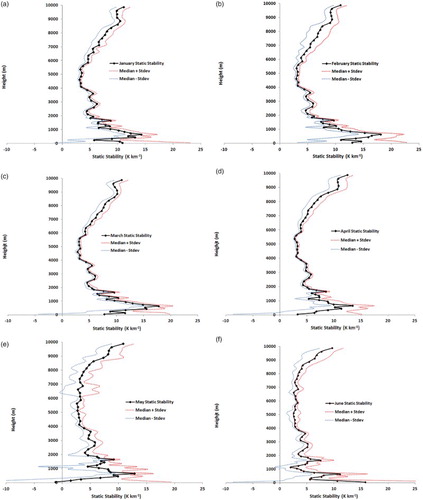
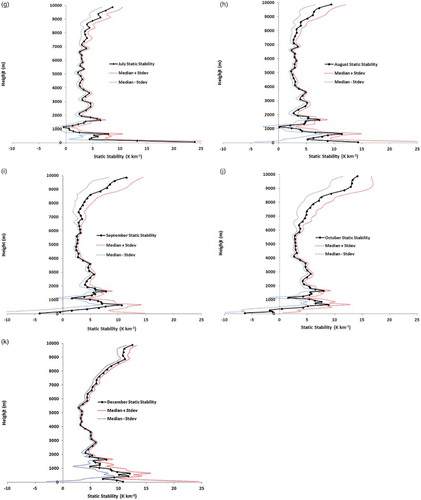
With static stability expressed in kelvins per kilometre, σ > 9.8 identifies an inversion; 0 < σ < 9.8 identifies a stable layer with temperature decreasing with height; σ = 0 identifies a layer with neutral stability; and σ < 0 identifies an unstable layer with temperature decreasing with height at a rate greater than the dry adiabatic lapse rate. Using the median static stability profiles, the height of each month's tropopause was identified by the presence of a layer with σ > 7.8 K km⁻¹ in the upper troposphere, in keeping with the WMO (1986) definition. The average static stabilities of the lower troposphere, arbitrarily set at 2000 to 5000 m, and of the upper troposphere, between 5000 and 8000 m, were determined for each month. Near-surface inversions were identified in the monthly static stability profiles, and their elevations, depths and strengths, defined by the average static stability through the layer or layers, were extracted.

4 Results and discussion

Similarities in the thermal structure of the troposphere over the southeastern Beaufort Sea–Amundsen Gulf region of the western maritime Arctic within seasons and differences across seasons can be seen in the monthly median static stability profiles (Fig. 1). These profiles reveal the seasonal evolution of the thermal character of the Arctic air mass (Penner, 1955) and the complex thermal structure of the ABL over this marine region where the variability in static stability was much greater than in the free atmosphere during our composite year (Raddatz et al., 2012, 2014).

a Atmospheric Boundary Layer

The height, depth, and strength (with standard deviations in brackets) of the median near-surface inversion layer or layers for each month are listed in Table 2. The median static stability profiles for December, January, February, and March indicated deep (tops ≥1000 m) and fairly strong (11–14 K km⁻¹) inversions that were surface based or slightly elevated. The median profile for April and the median profile for May each revealed an inversion elevated above a thermal internal boundary layer (Arya, 2001; Garratt, 1990; Raddatz et al., 2011, 2012). Throughout the winter and early spring, the hourly static stabilities of the surface layers, within one standard deviation of the median, ranged from very stable to unstable. The occurrence of weakly stable to unstable surface layers in the envelope of static stability profiles within one standard deviation of the median profiles for December, January, and March, as well as the presence of thermal internal boundary layers in the median April and May static stability profiles, have been linked to sensible heat flux from the unconsolidated sea-ice surface of Amundsen Gulf (Raddatz et al., 2012). Although the total sea-ice cover was very high throughout the winter and early spring (≈97% until mid-May), it was generally unconsolidated (i.e., the sea ice had an inter-ice-floe lead network and polynya—a non-linearly shaped area of open water or new and young sea ice ≤0.3 m thick). Using the MWR temperature profiles for 520 hours with clear skies from January to April 2008 and the integral profile method, Raddatz et al. (2013a) estimated that the mesoscale upward sensible heat fluxes from the unconsolidated sea-ice surface ranged from 0 to 183 W m⁻²; the median was approximately 11 W m⁻², the mean approximately 21 W m⁻², and the mode approximately 0 W m⁻².

Table 2. Heights, depths, and strengths (with standard deviations in brackets) of near-surface inversions in median profiles.

Month	Near-Surface Inversions (m)	Strength σ (K km^−1)
January 2008	0–200 400–1000	10.6 (9.2) 12.2 (2.5)
February 2008	0–1100	13.8 (4.7)
March 2008	100–1000	13.4 (3.3)
April 2008	400–800	11.2 (4.2)
May 2008	400–700	10.6 (3.6)
June 2008	0–200 500–600	13.2 (17.3) 11.1 (5.2)
July 2008	0–200	18.5 (11.5)
August 2009	0–100 600–700	14.3 (18.6) 11.4 (3.5)
September 2009	600–700	10.6 (3.6)
October 2009	No inversion	—
November 2008 and 2009	Insufficient data	—
December 2007	0–100 400–700	10.7 (13.6) 11.2 (3.0)

From mid-May onward, the total sea-ice cover of Amundsen Gulf steadily declined to its summer minimum of less than 20%. Relatively shallow (≤200 m) but fairly strong (≥13 K km⁻¹) surface inversions were apparent in the median static stability profiles for June, July, and August. Elevated inversions were also found in June and August. The surface inversions have been attributed to the downward flux of sensible heat from the atmosphere to the surface (Raddatz et al., 2012) because the nearly open water of Amundsen Gulf is often colder than the air flow (Gultepe, Isaac, Williams, Marcotte, & Strawbridge, 2003; Raddatz et al., 2012). Using the MWR temperature profiles for seven days from June to July 2008 and a variation of the integral profile method, Raddatz et al. (2012) estimated that the mesoscale downward sensible heat fluxes during this period ranged from −2 to −45 W m⁻²; the mean was −19 W m⁻².

Unstable surface layers were evident in the median profiles for the seasonal transition months of May (0–100 m; average σ = −1.2 ± 20.5 K km⁻¹), September (0–200 m; average σ = −2.4 ± 14.2 K km⁻¹), and October (0–300 m; average σ = −3.2 ± 5.8 K km⁻¹). There were elevated inversions in both May and September but not in October when the unstable surface layer was the deepest. The unstable surface layers suggest cold outbreaks with surface water temperatures warmer than the air flow. Sensible heat fluxes have not been calculated for these seasonal transition periods of the composite year.

The southeastern Beaufort Sea–Amundsen Gulf marine region has a large seasonal swing in sea-ice cover from more than 90% in winter to less than 20% in summer (Galley et al., 2008; Raddatz et al., 2012), and in the composite year, it was evident that equilibrium was generally established between the ABL and the unconsolidated sea-ice surface of Amundsen Gulf (Raddatz et al., 2012). Each passage of a migratory frontal-wave cyclone disrupted this equilibrium; however, it was quickly re-established after the passage of the baroclinic disturbance (Raddatz et al., 2014). In the composite year, 10 deep (<100 kPa) pressure minima were recorded in Amundsen Gulf and identified as baroclinic disturbances (23 January, 6 March, 14 April, 15 May, 21 July, 5 September, 11 September, 18 September, 1 November, and 8 November). The relatively high number of deep pressure minima in autumn is consistent with the findings of Hudak and Young (2002). They found that the average (1970–1995) number of storms in the Beaufort Sea region in the June to November period was 14 with a standard deviation of 5.

b Free Atmosphere

The monthly static stability profiles for the free atmosphere (2000–10,000 m) revealed an annual cycle (Table 3). Although the free atmosphere was stable throughout the annual cycle, the average static stability of the lower troposphere (2000–5000 m) was a minimum of 3.3 ± 0.5 K km⁻¹ in July and a maximum of 4.5 ± 0.5 K km⁻¹ in January and February. In the upper troposphere (>5000–8000 m), the average static stability was a minimum of 2.9 ± 0.6 K km⁻¹ in June and August and a maximum of 5.3 ± 0.8 K km⁻¹ in January. The average static stability of the upper troposphere was greater than the lower troposphere from December through March, but this pattern was reversed from May through September. The upper tropospheric and lower tropospheric static stabilities were similar in April and October. The winter-to-summer difference in static stability of the free atmosphere over the southeastern Beaufort Sea–Amundsen Gulf marine region was minimal in spite of the extreme annual cycle of solar insolation. The sun remains below the horizon from late November to late January, thus the incident shortwave radiation at the top of the atmosphere is effectively zero for a month on either side of the winter solstice. From late May to late July, the sun is constantly above the horizon with the incident shortwave radiation at the top of the atmosphere on the summer solstice exceeding 600 W m⁻². Thus, there is a dramatic seasonal swing from a large net radiative heat loss in winter to a large net gain in summer, and the results for the composite year suggest that in winter in situ radiative heat flux divergence resulted in somewhat more intense cooling at upper levels than at lower levels (Overland, 2009; Overland & Guest, 1991). The reversal of this pattern in the warmer months of the composite year may have been influenced by advection accompanying the passage of transient baroclinic disturbances (Held, 1982; Junkes, 2000).

Table 3. Average monthly median static stabilities (with standard deviations in brackets) of the lower troposphere (2000–5000 m) and upper troposphere (>5000–8000 m), plus the monthly median heights of the tropopause.

Month	Average σ (K km^−1) Lower Troposphere	Average σ (K km^−1) Upper Troposphere	Tropopause Height (m)
January 2008	4.5 (0.5)	5.3 (0.8)	8000
February 2008	4.5 (0.5)	4.7 (1.2)	8500
March 2008	4.4 (0.4)	5.0 (0.6)	8000
April 2008	4.2 (0.3)	4.3 (0.7)	8500
May 2008	4.2 (1.1)	3.1 (1.5)	9000
June 2008	3.7 (0.8)	2.9 (0.6)	9750
July 2008	3.3 (0.5)	3.1 (0.5)	9750
August 2009	3.6 (0.5)	2.9 (0.4)	9750
September 2009	3.9 (0.5)	3.0 (0.6)	9000
October 2009	4.0 (0.5)	4.1 (1.1)	8500
November 2008 and 2009	Insufficient data	Insufficient data	Insufficient data
December 2007	4.3 (0.3)	4.9 (0.5)	8000

The monthly median heights of the tropopause (Table 3) also had an annual cycle (Kanter, 1967). The maximum of 9750 m occurred in June, July, and August. The minimum tropopause height of 8000 m occurred in December, January, and March. The lower tropopause heights in winter likely coincided with the presence of the semi-permanent Arctic high pressure centre (Serreze & Barrett, 2011). This shallow cold-core anticyclone is attributed to in situ radiative heat flux divergence that results in intense cooling giving cold, dry, and mainly clear weather (Overland & Guest, 1991). Migratory cyclones (Penner, 1955; Raddatz et al., 2014; Serreze & Barry, 1988; Serreze, Lynch, & Clark, 2001) occasionally bring anomalously warmer and moister weather to the western maritime Arctic, and as noted ten deep cyclones were recorded in the composite year. From the frequency distribution of downwelling longwave radiation and the hourly time series of several atmospheric state variables, Raddatz et al. (2015) determined that during the extended winter (December to March) the cold-core anticyclone was present approximately 69% of the time, and baroclinic cyclones were present approximately 24% of the time. These results are consistent with those obtained by Stramler, Del Genio, and Rossow (2011) from the 1977–1998 winter Surface Heat Budget of the Arctic (SHEBA) net longwave radiation data for the Beaufort Sea, and for the 2005/06 to 2009/10 winter downwelling longwave radiation data for Sachs Harbour on nearby Banks Island. Similar longwave radiation frequency distributions at these sites, with different surface characteristics, suggest that the occurrence-pattern of the winter cold-core anticyclone and baroclinic cyclones was synoptically driven.

As noted, in addition to synoptic-scale variability, the southeastern Beaufort Sea–Amundsen Gulf marine region has extreme annual cycles of solar insolation and sea-ice cover. The sun remains below the horizon from late November to late January (Overland, 2009), and the sea-ice cover decreases from more than 90% in winter to less than 20% in summer (Galley et al., 2008; Raddatz et al., 2012). Thus, the seasonal cycles of static stability in the free atmosphere and the seasonal cycle in the height of the tropopause can be attributed to regional as well as synoptic-scale forcing.

Static stability is widely used to classify the thermal stability of the atmosphere, accounting for its importance to mesoscale convection. On the synoptic-scale, static stability is an important coefficient of vertical velocity in the equation governing cyclonic development (Bluestein, 1992; Gates, 1961). Cyclonic development in the lower troposphere has been shown to result from an imbalance between vorticity advection at the level of non-divergence and the Laplacian of the terms that contribute to the local rate of change of temperature: (i) horizontal advection, (ii) adiabatic change, and (iii) change due to non-adiabatic heating or cooling (Petterssen, 1956a, 1956b). Because the influence of adiabatic temperature change on cyclonic development essentially depends on static stability times vertical velocity, development will preferentially take place where and when there is a minimum in the stability of the normally stable lower troposphere—provided that other conditions are favourable. This analysis revealed that the average static stability of the lower troposphere (2000–5000 m) over the southeastern Beaufort Sea–Amundsen Gulf region in our composite year had a minimum of 3.3 K km⁻¹ in July and a maximum of 4.5 K km⁻¹ in January and February. This implies that over the western maritime Arctic, all else being equal, cyclonic development is more strongly favoured by the adiabatic term in summer than in winter.

5 Conclusions

The characterization of the static stability of the troposphere over the western maritime Arctic remains limited in spite of its significance to both atmospheric thermodynamics and dynamics. Field observations of MWR temperature profiles from the IPY-CFL system study (late November 2007 to mid-July 2008) and the ArcticNet field campaign (mid-July to early November 2009) provided a unique opportunity to describe the static stability of the troposphere and its annual cycle over the southeastern Beaufort Sea–Amundsen Gulf region. This analysis contributes to the understanding of the atmospheric thermodynamics and dynamics of this data-sparse region by providing a snapshot of the area's current atmospheric state.

Notably, the monthly median ABL (<2000 m) static stability profile for April and the profile for May clearly revealed an inversion elevated above a thermal internal boundary layer, whereas the median summer static stability profiles, especially July's, had very strong surface-based inversions. These profiles have been linked to the seasonal evolution of the sea-ice cover of Amundsen Gulf. The monthly static stability profiles for the free atmosphere (2000–10,000 m) revealed an annual cycle. The average static stability of the lower troposphere (2000–5000 m) was a minimum of 3.3 ± 0.5 K km⁻¹ in July and a maximum of 4.5 ± 0.5 K km⁻¹ in January and February. In the upper troposphere (>5000–8000 m), the average static stability was a minimum of 2.9 ± 0.6 K km^–1 in June and August and a maximum of 5.3 ± 0.8 K km⁻¹ in January. The monthly median heights of the tropopause also had an annual cycle. The maximum of 9750 m occurred in June, July, and August. The minimum tropopause height of 8000 m occurred in December, January, and March. The seasonal cycles of static stability in the free atmosphere and the seasonal cycle in the height of the tropopause can be attributed to regional as well as synoptic forcing.

Acknowledgement

This work is a contribution to the Arctic Science Partnership (ASP).

Disclosure statement

No potential conflict of interest was reported by the authors.

References

- American Meteorological Society (AMS). (2000). Glossary of meteorology. Boston, MA: AMS. Retrieved from http://glossary.ametsoc.org/wiki/Main_Page
- Arya, S. P. (2001). Introduction to micrometeorology (2nd ed.). San Diego, CA: Academic Press.
- Barber, D. G., Asplin, M. G., Gratton, Y., Lukovich, J. V., Galley, R. J., Raddatz, R. L., & Leitch, D. (2010). The international polar year (IPY) Circumpolar Flaw Lead (CFL) system study: Overview and the physical system. Atmosphere-Ocean, 48, 225–243.
- Barber, D. G., & Hanesiak, J. M. (2004). Meteorological forcing of sea ice concentrations in the southern Beaufort Sea over the period 1979 to 2000. Journal of Geophysical Research, 109, C06014. doi:10.1029/2003JC002027
- Bethan, S., Vaughan, G., & Reid, S. J. (1996). A comparison of ozone and thermal tropopause heights and the impact of tropopause definition on quantifying the ozone content of the troposphere. Quarterly Journal of the Royal Meteorological Society, 122, 929–944. doi: 10.1002/qj.49712253207
- Bluestein, H. B. (1992). Synoptic-dynamic meteorology in midlatitudes: Volume I: Principles of kinematics and dynamics. Don Mills, Ontario: Oxford University Press Canada.
- Candlish, L. M., Raddatz, R., Asplin, M., & Barber, D. G. (2012). Atmospheric temperature and absolute humidity profiles over the Beaufort Sea and Amundsen Gulf from a microwave radiometer. Journal of Atmospheric and Oceanic Technology, 29, 1182–1201. doi:10.1175/JTECH-D-10-05050.1
- Environment Canada (EC). (2011). The Canadian Ice Service Archive (CISDA) [Data]. Canadian Ice Service. Retrieved from http://dynaweb.cis.ec.gc.ca/Archive10/?lang=en
- Frierson, D. M. W. (2006). Robust increases in midlatitude static stability in simulations of global warming. Geophysical Research Letters, 33, L24816. doi:10.1029/2006GL027504
- Gaffard, C., Nash, J., Walker, E., Hewison, T. J., Jones, J., & Norton, E. G. (2008). High time resolution boundary layer description using combined remote sensing instruments. Annales Geophysicae, 26, 2597–2612. doi: 10.5194/angeo-26-2597-2008
- Galley, R. J., Key, E., Barber, D. G., Hwang, B. J., & Ehn, J. (2008). Spatial and temporal variability of sea ice in the southern Beaufort Sea and Amundsen Gulf: 1980–2004. Journal of Geophysical Research, 113, C05S95. doi:10.1029/2007JC004553
- Garratt, J. R. (1990). The internal boundary layer: A review. Boundary-Layer Meteorology, 50, 171–203. doi: 10.1007/BF00120524
- Gates, W. L. (1961). Static stability measures in the atmosphere. Journal of Meteorology, 18, 526–533. doi: 10.1175/1520-0469(1961)018<0526:SSMITA>2.0.CO;2
- Güldner, J., & Spänkuch, D. (2001). Remote sensing of the thermodynamic state of the atmospheric boundary layer by ground-based microwave radiometry. Journal of Atmospheric and Oceanic Technology, 18, 925–933. doi: 10.1175/1520-0426(2001)018<0925:RSOTTS>2.0.CO;2
- Gultepe, I., Isaac, G. A., Williams, A., Marcotte, D., & Strawbridge, K. B. (2003). Turbulent heat fluxes over leads and polynyas, and their effects on Arctic clouds during FIRE.ACE: Aircraft observations for April 1998. Atmosphere-Ocean, 41, 15–34. doi: 10.3137/ao.410102
- Gultepe, I., Kuhn, T., Pavolonis, M., Calvert, C., Gurka, J., Heymsfield, A. J., … Bernstein, B. (2014). Ice fog in Arctic during FRAM–Ice Fog Project: Aviation and nowcasting applications. Bulletin of the American Meteorological Society, 95, 211–226. doi:http://dx.doi.org/10.1175/BAMS-D-11-00071.1
- Held, I. M. (1982). On the height of the tropopause and the static stability of the troposphere. Journal of the Atmospheric Sciences, 39, 412–417. doi: 10.1175/1520-0469(1982)039<0412:OTHOTT>2.0.CO;2
- Homeyer, C. R., Bowman, K. P., & Pan, L. L. (2010). Extratropical tropopause transition layer characteristics from high-resolution sounding data. Journal of Geophysical Research, 115, D13108. doi:10.1029/2009JD013664
- Hooper, D. A., & Arvelius, J. (2000). Monitoring of the Arctic winter tropopause: A comparison of radiosonde, ozonesonde and MST radar observations. In Proceedings of the ninth international workshop on technical and scientific aspects of MST radar combined with COST76 final profiler workshop, B. Edwards (Ed.), pp. 385–388, Sci. Comm. Boulder, Colorado: On Sol.-Terr. Phys. Secr. and Meteo France.
- Hudak, D. R., & Young, J. M. C. (2002). Storm climatology of the southern Beaufort Sea. Atmosphere-Ocean, 40, 145–158. doi: 10.3137/ao.400205
- Junkes, M. N. (2000). The static stability of the Midlatitude Troposphere: The relevance of moisture. Journal of the Atmospheric Sciences, 57, 3050–3057. doi: 10.1175/1520-0469(2000)057<3050:TSSOTM>2.0.CO;2
- Kanter, A. J. (1967). Tropopause height variations over Canada. Journal of Applied Meteorology, 6, 593–595. doi: 10.1175/1520-0450(1967)006<0593:THVOC>2.0.CO;2
- Liljegren, J., Lesht, B., Kato, S., & Clothiaux, E. (2001). Initial evaluation of profiles of temperature, water vapor, and cloud liquid water from a new microwave profiling radiometer. 11th Atmospheric Radiation Measurement (ARM) Program Science Team Meeting, Atlanta, Ga., Dep. of Energy, Washington, D. C., 19–23 March. Retrieved from http://radiometrics.com/downloads/
- Nagurny, A. P. (1998). Climatic characteristics of the tropopause over the Arctic Basin. Annales Geophysicae, 16, 110–115. doi: 10.1007/s00585-997-0110-6
- Overland, J. E. (2009). Meteorology of the Beaufort Sea. Journal of Geophysical Research, 114, C00A07. doi:10.1029/2008JC004861
- Overland, J. E., & Guest, P. S. (1991). The Arctic snow and air temperature budget over sea ice during winter. Journal of Geophysical Research, 96, 4651–4662. doi: 10.1029/90JC02264
- Penner, C. M. (1955). A three-front model for synoptic analyses. Quarterly Journal of the Royal Meteorological Society, 81, 89–91. doi: 10.1002/qj.49708134710
- Petterssen, S. (1956a). Weather analysis and forecasting (2nd ed., Vol. I). Motion and motion systems. Toronto: McGraw-Hill Canada.
- Petterssen, S. (1956b). Weather analysis and forecasting (2nd ed., Vol. II). Weather and weather systems. Toronto: McGraw-Hill Canada.
- Pratt, R. (1985). Review of radiosonde humidity and temperature errors. Journal of Atmospheric and Oceanic Technology, 2, 404–407. doi:http://dx.doi.org/10.1175/1520-0426(1985)002<0404:RORHAT>2.0.CO;2
- Raddatz, R. L., Asplin, M. G., Candlish, L., & Barber, D. G. (2011). General characteristics of the atmospheric boundary layer in a flaw lead polynya region for winter and spring. Boundary-Layer Meteorology, 138, 321–335. doi:10.1007/s10546-010-9557-1
- Raddatz, R. L., Galley, R. J., & Barber, D. G. (2012). Linking the atmospheric boundary layer to the Amundsen Gulf sea-ice cover: A mesoscale to synoptic-scale perspective from winter to summer 2008. Boundary-Layer Meteorology, 142, 123–148. doi:10.1007/s10546-011-9669-2
- Raddatz, R. L., Galley, R. J., Candlish, L. M., Asplin, M. G., & Barber, D. G. (2013a). Integral profile estimates of sensible heat flux from an unconsolidated sea-ice surface. Atmosphere-Ocean, 51, 135–144. doi:10.1080/07055900.2012.759900
- Raddatz, R. L., Galley, R. J., Candlish, L. M., Asplin, M. G., & Barber, D. G. (2013b). Integral profile estimates of latent heat flux under clear skies at an unconsolidated sea-ice surface. Atmosphere-Ocean, 5, 239–248. doi:10.1080/07055900.2013.785383
- Raddatz, R. L., Galley, R. J., Candlish, L. M., Asplin, M. G., & Barber, D. G. (2013c). Water vapour over the western maritime Arctic: Surface inversions, intrusions and total column. International Journal of Climatology, 33, 1436–1443. doi:10.1002/joc.3524.
- Raddatz, R. L., Galley, R. J., Else, B. G., Papakyriakou, T. N., Asplin, M. G., Candlish, L. M., & Barber, D. G. (2014). Western Arctic cyclones and equilibrium between the atmospheric boundary layer and the sea surface. Atmosphere-Ocean, 52, 125–141. doi:10.1080/07055900.2014.890921
- Raddatz, R. L., Papakyriakou, T. N., Else, B. G., Asplin, M. G., Candlish, L. M., Galley, R. J., & Barber, D. G. (2015). Downwelling longwave radiation and atmospheric winter states in the western maritime Arctic. International Journal of Climatology, 35, 2339–2351. doi:10.1002/joc.4149
- Schmidlin, F. J. (1988). WMO international radiosonde comparison, phase II final report, instruments and observing methods (Rep. 29, WMO/TD-No. 312). Geneva: World Meteorological Organization.
- Seidel, D. J., & Randel, W. J. (2006). Variability and trends in the global tropopause estimated from radiosonde data. Journal of Geophysical Research, 111, D21101. doi:10.1029/2006JD007363
- Serreze, M. C., & Barrett, A. P. (2011). Characteristics of the Beaufort Sea high. Journal of Climate, 24, 159–182. doi: 10.1175/2010JCLI3636.1
- Serreze, M. C., & Barry, R. G. (1988). Synoptic activity in the Arctic basin, 1979–85. Journal of Climate, 1, 1276–1295. doi: 10.1175/1520-0442(1988)001<1276:SAITAB>2.0.CO;2
- Serreze, M. C., Lynch, A. H., & Clark, M. P. (2001). The Arctic frontal zone as seen in the NCEP–NCAR reanalysis. Journal of Climate, 14, 1550–1567. doi: 10.1175/1520-0442(2001)014<1550:TAFZAS>2.0.CO;2
- Solheim, F., Godwin, J. R., Westwater, E. R., Han, Y., Keihm, S. J., March, K., & Ware, R. (1998). Radiometric profiling of temperature, water vapor, and cloud liquid water using various inversion methods. Radio Science, 33, 393–404. doi: 10.1029/97RS03656
- Son, S-W., Polvani, L. M., Waugh, D. W., Birner, T., Akiyoshi, T. H., Garcia, R. R., … Rozanov, E. (2009). The impact of stratospheric ozone recovery on tropopause height trends. Journal of Climate, 22, 429–445. doi: 10.1175/2008JCLI2215.1
- Stramler, K., Del Genio, A. D., & Rossow, W. B. (2011). Synoptically driven Arctic winter states. Journal of Climate, 24, 1747–1762. doi:10.1175/2010JCL13817.1
- Ware, R., Carpender, R., Güldner, J., Liljegren, J., Nehrkorn, T., Solhelm, F., & Vandenberghe, F. (2003). A multichannel profiler of temperature, humidity, and cloud liquid. Radio Science, 38, 8079. doi:10.1029/2002RS002856
- World Meteorological Organization (WMO). (1986). Atmospheric ozone 1985 (Tech. Rep. 16). World Meteorological Organisation: Geneva, Switzerland.