Storm Surges in the Strait of Georgia Simulated with a Regional Model

Abstract

The Strait of Georgia is a large, semi-enclosed body of water between Vancouver Island and the mainland of British Columbia connected to the Pacific Ocean via Juan de Fuca Strait at the south and Johnstone Strait at the north. During the winter months, coastal communities along the Strait of Georgia are at risk of flooding caused by storm surges, a natural hazard that can occur when a strong storm coincides with high tide. This investigation produces storm surge hindcasts using a three-dimensional numerical ocean model for the Strait of Georgia and the surrounding bodies of water (Juan de Fuca Strait, Puget Sound, and Johnstone Strait) collectively known as the Salish Sea. The numerical model employs the Nucleus for European Modelling of the Ocean architecture in a regional configuration. The model is evaluated through comparisons of tidal elevation harmonics and storm surge with observations. Important forcing factors contributing to storm surges are assessed. It is shown that surges entering the domain from the Pacific Ocean make the most significant contribution to surge amplitude within the Strait of Georgia. Comparisons between simulations and high-resolution and low-resolution atmospheric forcing further emphasize that remote forcing is the dominant factor in surge amplitudes in this region. In addition, local wind patterns caused a slight increase in surge amplitude on the mainland side of the Strait of Georgia compared with Vancouver Island coastal areas during a major wind storm on 15 December 2006. Generally, surge amplitudes are found to be greater within the Strait of Georgia than in Juan de Fuca Strait.

Résumé

[Traduit par la rédaction] Le détroit de Georgia est un vaste plan d'eau semi-fermé situé entre l’île de Vancouver et la Colombie-Britannique continentale. Il est relié à l'océan Pacifique par le détroit Juan de Fuca, au sud, et par le détroit Johnstone, au nord. Durant l'hiver, les communautés côtières habitant le long du détroit de Georgia risquent de subir les inondations qu'engendrent les ondes de tempête, un danger naturel qui se manifeste lorsqu'une forte tempête survient à marée haute. Cette étude porte sur la production de prévisions a posteriori d'ondes de tempête que simule un modèle numérique océanique tridimensionnel pour le détroit de Georgia et les plans d'eau adjacents (le détroit Juan de Fuca, Puget Sound et le détroit de Johnstone), connus collectivement sous le nom de « mer des Salish ». Le modèle numérique utilise l'architecture du Nucleus for European Modelling of the Ocean selon une configuration régionale. Nous validons le modèle en comparant les harmoniques de hauteurs de marée et les ondes de tempête avec les observations. Nous examinons en outre les forçages qui contribuent aux ondes de tempête. Il semble que les ondes de tempête qui entrent dans le domaine à partir de l'océan Pacifique contribuent le plus à l'amplitude des ondes dans le détroit de Georgia. Les comparaisons entre les simulations et des forçages atmosphériques à haute et à basse résolutions démontrent qu'un forçage éloigné domine l'amplitude des ondes dans cette région. De plus, pour la tempête majeure de vent survenue le 15 décembre 2006, la configuration des vents locaux produit une légère augmentation de l'amplitude de l'onde du côté continental du détroit de Georgia comparativement aux régions côtières de l’île de Vancouver. En général, l'amplitude des ondes de tempête reste plus prononcée dans le détroit de Georgia que dans le détroit Juan de Fuca.

KEYWORDS:

• storm surge
• Strait of Georgia
• Salish Sea
• numerical modelling
• spatial variation

1 Introduction

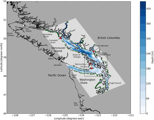
The Strait of Georgia is a strongly stratified, semi-enclosed body of water located between Vancouver Island and the mainland of British Columbia (Thomson, 1981). It is part of a larger system of waterways collectively known as the Salish Sea and is connected to the Pacific Ocean via Juan de Fuca Strait and Johnstone Strait (Fig. 1). At its southern end, the Strait of Georgia is connected to Juan de Fuca Strait through several passages, the largest being Haro Strait. The San Juan and Gulf Islands are scattered throughout these passages where complex bathymetry and steep topographic slopes induce vigorous tidal mixing (Thomson, 1981). Mixed diurnal and semi-diurnal tides are found throughout most of the Salish Sea but a semi-diurnal amphidrome is present near Victoria, where the tides are mainly diurnal (Thomson, 1981). This system is home to several large coastal communities, such as Vancouver and Victoria, serves as a waterway for commercial traffic and recreational use, and supports a large and active fishing industry.

Fig. 1 Model domain (light grey area) including bathymetry, rivers (green circles), and storm surge locations of interest (red stars). The black rectangle represents the region displayed in Fig. 2.

Many coastal communities in the Strait of Georgia are at risk of flooding and property damage caused by storm surges, a natural hazard arising from the combination of a strong wind storm and high tide. The low atmospheric pressure associated with a storm acts as an inverse barometer elevating the sea level. This effect, in combination with strong winds pushing water up against the coast, can cause flooding, particularly if the storm occurs during an unusually high tide. There is also a small contribution to increased sea level from positive sea surface height anomalies propagating northward from the equator along the eastern Pacific coast during El Niño years (Strub & James, 2002). Communities along the Strait of Georgia are particularly susceptible to storm surges in winter when there is an increased propensity for storms and a higher sea level caused by southeasterly winds and geostrophic adjustment (Danard, Munro, & Murty, 2003). In the summer months, the wind direction changes to northwesterly and mean sea level is lower. In British Columbia waters, the largest tidal ranges occur in June and December at the summer and winter solstices (Thomson, 1981). The highest water levels are observed in the winter around the perigean springtide or “King” tide, when the sun and moon are aligned with the Earth and the moon is at its perigee. Storm surges in the Strait of Georgia are typically observed between November and February (Forseth, 2012). Flooding caused by a storm surge is most likely to occur during a high spring tide (Abeysirigunawardena, Smith, & Taylor, 2011).

Coastal communities can prepare for and respond to storm surge hazards using predictions from storm surge models to determine whether flooding conditions are probable. As with coastal ocean models, some of the complexity of a storm surge model depends on the properties of the geographic location of interest. In shallow regions, it is important to include the effects of wetting and drying, which allows grid cells to alternate between land and water depending on the modelled sea surface height and depth (Hubbert & McInnes, 1999; Weisberg & Zheng, 2006). Other regions require modelling over a very large domain because non-local effects from the open sea may influence surge propagation (Lane & Walters, 2009; Mercer, Sheng, Greatbatch, & Bobanović, 2002; Weisberg & Zheng, 2006). Such large domains typically use nested or unstructured grids to resolve the details of complicated coastlines. Appropriate treatment of rivers (Flather, 1994), accurate bathymetry, and the inclusion of surface waves (Xu, Zhang, Shen, & Li, 2010) have also been identified as important. Most of these models neglect the effects of stratification by treating the ocean as having a constant temperature and salinity. An accurate forecast of the meteorological conditions at the ocean surface is, of course, essential in the generation of useful storm surge forecasts.

Storm surge modelling in the Strait of Georgia dates back to P. Crean, Murty, and Stronach (1988) who used a barotropic finite difference model. Their work is highlighted in reviews of storm surges in Canadian waters (Danard et al., 2003; Murty, Venkatesh, Danard, & El-Sabh, 1995). Compared with eastern Canada (Bernier & Thompson, 2006, 2007, 2010; Bobanović, Thompson, Desjardins, & Ritchie, 2006; Gray et al., 1984; Ma, Han, & de Young, 2015), relatively little has been published on storm surge modelling on the west coast of Canada in recent years. However, a storm surge forecasting program is currently operating over a domain that covers the entire British Columbia coastline (Tinis, 2014). Further, a statistical overview of past surge events in British Columbia waters suggests an increase in extreme water level events during warm El Niño periods (Abeysirigunawardena et al., 2011).

The early modelling work of P. Crean et al. (1988), P. B. Crean, Murty, and Stronach (1988), and Stronach, Backhaus, and Murty (1993) developed a series of models covering Juan de Fuca Strait, the Strait of Georgia, and Puget Sound using a finite difference discretization of the equations of motion. These models pointed to an important connection between a model's bottom friction parametrization and the location and amplitude of the M₂ amphidrome. These authors found that a local increase in the bottom friction coefficient, typically from 0.002 to 0.004 in the baroclinic model, especially in the vicinity of Haro Strait, was necessary in order to adequately reproduce the observed M₂ tidal amplitudes and phase lags in the Strait of Georgia (Stronach et al., 1993).Without local adjustments to the bottom friction the model's M₂ amplitudes were too low, and the M₂ tidal phases were too large in the Strait of Georgia (P. Crean et al., 1988). Local adjustments to bottom friction were applied in both the barotropic and baroclinic models. Other studies over a similar domain, such as the barotropic finite element model of Foreman, Walters, Henry, Keller, and Dolling (1995), have avoided local increases in bottom friction although their domain did not include Puget Sound or the northern Strait of Georgia. Foreman, Sutherland, and Cummins (2004) assimilated tide gauge harmonics to study M₂ tidal dissipation without local changes to the bottom friction in a two-dimensional finite element model that did not include baroclinic effects.

More recently, modelling studies have focused on baroclinic features. Masson and Cummins (2004) used the Princeton Ocean Model (POM) in a regional mode to examine the seasonal variability of deep water properties in the Strait of Georgia and noted a strong sensitivity to vertical mixing over the sills. This model employed a sigma or terrain-following vertical coordinate system leading to spurious diapycnal mixing because, numerically, the lateral mixing is computed on sigma levels which may intersect isopycnals in the presence of steep topography. Sutherland, MacCready, Banas, and Smedstad (2011) employed the Regional Ocean Modelling System (ROMS) to study estuarine circulation in the Salish Sea with a model domain that extended outside Juan de Fuca Strait into the Pacific Ocean and up to the northern Strait of Georgia. They noted that their semi-diurnal amplitudes were generally too low. An updated version of this model with added biogeochemical components and an extended domain produced higher-than-observed surface temperatures in Juan de Fuca Strait, suggesting too little mixing within the Salish Sea (Giddings et al., 2014). Smaller domains have also been considered; notably, the passageways through the Discovery Islands north of the Strait of Georgia have been modelled baroclinically by Foreman et al. (2012) with the Finite Volume Coastal Ocean Model (FVCOM) pointing to difficulties in reproducing baroclinic currents on their grid. Accurate reproduction of observed tidal amplitudes and phases and appropriate treatment of mixing is a recurring difficulty in modelling this region.

This article presents the development of a three-dimensional numerical ocean model for the Strait of Georgia and its skill in simulating storm surge hindcasts. The main goals are to identify the forcing factors that contribute most significantly to storm surges in the Strait of Georgia, to examine the spatial distribution of the storm surges, and to evaluate the performance of a new model of this region. To complement previous barotropic storm surge modelling in this region, this model has a higher resolution and includes the effects of stratification and rivers. However, wetting and drying are not represented. Model evaluation has focused on regions where the near-coast slopes are steep, so wetting and drying effects are believed to be unimportant. A detailed overview of the model configuration and domain is provided in Section 2, which also describes open and surface boundary conditions as well as choices in grid structure and mixing parametrizations. Next, Section 3 presents an evaluation of model performance through comparisons of tidal amplitudes and phases with observations. The model's skill in producing storm surge hindcasts is assessed in Section 4. Several simulations comparing the effects of different forcing conditions are also discussed. Finally, a summary and discussion of future research goals are provided in Section 5.

2 Model description

We have used the Nucleus for European Modelling of the Ocean (NEMO) framework in its regional configuration (Madec et al., 2012) to develop an ocean model for the Salish Sea. The NEMO framework is a highly modular tool used for studying ocean physics, ocean–ice interactions, and the biogeochemical properties of the ocean. The ocean core of NEMO solves the three-dimensional hydrostatic equations of motion for an incompressible fluid under the Boussinesq approximation on a structured computational grid. Although these features are not being used in the present work, NEMO's options for grid nesting and biogeochemical coupling make it a useful tool for studying the complex physics and biogeochemical interactions within the Strait of Georgia. This work focuses on the physical configuration of the Salish Sea model, in particular, determining appropriate forcing and boundary conditions for accurate reproduction of tidal amplitudes and phases as well as storm surge elevations. Future work will include biogeochemical coupling and data assimilation. Version 3.4 of NEMO was used in this study. Other coastal modelling studies in the Northeast Atlantic (Maraldi et al., 2013) and the Mediterranean Sea (Brossier, Béranger, & Drobinski, 2012) have used NEMO successfully.

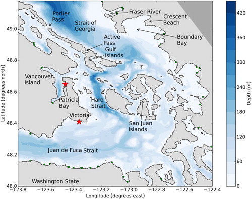
The modelled domain extends from Juan de Fuca Strait to Puget Sound to Johnstone Strait (Fig. 1). Bathymetry from the Cascadia physiography dataset (Haugerud, 1999) was smoothed to limit large changes in depth across grid cells, so that , where is the difference in depth between two adjacent grid cells, and is their average depth. For model stability, additional smoothing at the western boundary of Juan de Fuca Strait was imposed to achieve constant depth across the first ten grid cells inward from the open boundary. Depths between 0 and 4 m were set to 4 m. As depicted in Fig. 1, the numerical grid is rotated 29° counter-clockwise of north in order to maintain computational efficiency because currents within the Strait of Georgia are mainly aligned with this rotated axis. A magnified image of the complex passages through the San Juan and Gulf Islands is provided in Fig. 2.

Fig. 2 Model bathymetry and coastlines in the passages between the San Juan and Gulf Islands. See Fig. 1 for an explanation of the red stars.

The curvilinear orthogonal numerical grid was divided into 398 by 898 by 40 grid cells, which results in an almost uniform horizontal resolution with a grid spacing of approximately 440 m by 500 m. The 40 vertical -levels were gradually stretched in order to achieve higher resolution in the surface layer, with 1 m vertical grid spacing down to about 10 m in depth. Below 10 m the grid was stretched to a maximum grid spacing of 27 m in the lowest layer. At the bottom boundary, partial -levels were used in order to limit large changes in bathymetry across grid cells (Madec et al., 2012). Model constraints require that all passages be at least two grid points wide. This restriction required choices in either widening or closing narrow straits. In particular, Active Pass was closed and Porlier Pass was widened (Fig. 2). All these compromises are expected to have significant effects locally but minimal effects at the large scale.

In addition to the equations of motion, a prognostic equation for sea surface height is solved at each time step. The inclusion of the sea surface height equation requires a fairly restrictive time step because of the presence of high speed surface gravity waves. As such, the split-explicit time stepping algorithm is employed, in which the free surface and barotropic equations are solved with a smaller time step than that used for the other variables. The model baroclinic time step and barotropic time step are 10 and 2 s, respectively. Small vertical grid spacing and large vertical velocities in the Boundary Pass and Haro Strait regions impose a fairly restrictive baroclinic time step through the vertical Courant-Friedrichs-Lewy (CFL) condition.

The model includes two open boundaries that connect to the Pacific Ocean, the western boundary of Juan de Fuca Strait as well as Johnstone Strait at the north, both of which are forced with eight tidal constituents (K₁, O₁, P₁, Q₁, M₂, K₂, N₂, and S₂), temperature and salinity climatologies, and the sea surface height anomaly. Tidal heights and currents at grid points along the Juan de Fuca boundary were extracted from Webtide (Webtide, 2014), an online web prediction model that provides tidal predictions for the northeast Pacific Ocean based on work by Foreman, Crawford, Cherniawsky, Henry, and Tarbotto (2000). The Johnstone Strait boundary was forced with current and elevation tidal harmonics measured and calculated by Thomson and Huggett (1980) for the major M₂ and K₁ constituents. Additionally, O₁ and S₂ elevation harmonics from their measurements were employed. The remaining constituents were extrapolated from Webtide. At the western boundary, the tidal elevation and current forcing parameters were tuned for a good match with observations at locations within the Strait of Georgia, including Point Atkinson, Gibsons Landing, Winchelsea, and Halfmoon Bay. At the northern boundary, the tides were tuned for good matches at Yorke Island and Kelsey Bay. Further details on the tuning are provided in Appendix A.

Temperature and salinity at the Juan de Fuca boundary were taken from a weekly climatology that was created from results of a model covering the Salish Sea and the west coast of Vancouver Island (Masson & Fine, 2012). Masson and Fine's results, originally on -levels, were interpolated onto -levels and then onto the NEMO horizontal grid to give a two-dimensional forcing that varies with time. To prepare the climatology all years (1995–2008) were averaged and results, approximately every 15 days, were interpolated to a weekly climatology. The model is relaxed to the forced temperature and salinity over the 10 grid points (about 5 km) closest to the open boundaries, using a flow relaxation scheme (Engedahl, 1995). In the north, the seasonal climatologies of Thomson (1981) were used in the same manner.

The sea surface height anomaly (or remote forcing) was set uniformly across the mouth of Juan de Fuca Strait using values from the Tofino tide gauge (Fisheries and Oceans Canada, 2014) which is outside, but close to, the western boundary of the model domain (Fig. 1). A monthly climatology was produced using daily averages from 2000 to 2010, binning them by month, averaging and setting the annual mean to zero. For the storm surge simulations, hourly variations in sea surface height were used. These values are the Tofino tide gauge values with the tides removed. Tidal predictions were generated with the tidal analysis package called t_tide (Pawlowicz, Beardsley, & Lentz, 2002) using a time series from the year of the storm surge. A harmonic analysis was performed for 67 constituents. In order to prevent overpredicted constituents resulting from high surge years, the time series was first filtered by applying a tide-killing Doodson filter (Parker, 2007), and periods with large non-tidal amplitudes were removed. Long period constituents, such as Sa and Ssa, were not used in the tidal predictions because these constituents are often contaminated by non-tidal energy from seasonal meteorological trends. Further, constituents with a low signal-to-noise ratio were neglected. The storm surge simulations also used the sea surface height anomaly from Port Hardy, forced at the northern boundary in Johnstone Strait.

Although Tofino is not the closest tide gauge to the western boundary, we found that the surge conditions on the western coast of Vancouver Island and near the mouth of Juan de Fuca Strait are reasonably uniform as summarized in Table 1. Generally, surge amplitudes at Tofino are slightly larger and earlier than at Neah Bay and Bamfield. The remote forcing is applied uniformly across the open boundaries. Given the similarities between the surge amplitude and phase at Neah Bay and Bamfield, this seems to be a reasonable assumption. In support of this assumption, a geostrophic slope calculation with an estuarine velocity of 20 cm s⁻¹ would imply a difference of less than 5 cm between the northern and southern sides of Juan de Fuca Strait. In the future, this uniform specification of sea level at the western boundary will be relaxed by taking values from the solution of a large-scale forecasting model.

Table 1. Average peak surge amplitudes and delay in peak timing from Tofino at several tide gauges on the Pacific coast. Averages obtained over the five surge events hindcast in this article. A negative delay indicates that the peak surge occurred later than at Tofino.

Location	Mean surge amplitude (m)	Mean delay from Tofino (hr)
Port Hardy	0.491	−2.67
Winter Harbour	0.572	0.33
Tofino	0.707	—
Bamfield	0.658	−0.50
Neah Bay	0.658	−1.83
Toke Point	1.174	−2.83

The tidal forcing and non-tidal remote forcing were applied using the NEMO Flather scheme (Flather, 1994; Madec et al., 2012), a radiation scheme that allows disturbances to propagate out of the domain without reflections off the open boundary. The barotropic velocity component of the remote forcing was set to zero. At the west, the baroclinic velocities at the boundary were set equal to the values inside the boundary (zero-gradient boundary conditions). This scheme is not part of the core NEMO 3.4 (the version used here). Zero-gradient conditions were chosen because the baroclinic velocity at the mouth of Juan de Fuca Strait is primarily estuarine and thus set by density variations between the inside and outside of the domain. At the northern boundary, we chose the “no boundary condition” of NEMO that sets up an estuarine circulation by relaxing the temperature and salinity over a width of 10 grids to the seasonal climatology.

At coastal boundaries, a partial slip boundary condition (an approximation to no slip) was used. Partial slip allows the inclusion of the frictional effects of lateral boundaries without the restrictive resolution required to represent the lateral boundary layer under no slip conditions. A lateral eddy viscosity of 20 m² s⁻¹ parametrizes horizontal friction, and a lateral eddy diffusivity of 20.5 m² s⁻¹ was used. Bottom friction was represented by a quadratic law for the bottom momentum flux with drag coefficient . Vertical turbulence and mixing was calculated through the configuration of the generic length scale (GLS) turbulence closure (Umlauf & Burchard, 2003) with background vertical eddy viscosity and diffusivity set to 1 × 10⁻⁴ m² s⁻¹ and 1 × 10⁻⁵ m² s⁻¹, respectively. Details of the NEMO implementation of the partial slip lateral boundary condition, quadratic bottom friction law, and GLS turbulence closure scheme are provided in Madec et al. (2012).

The ocean surface is forced with momentum fluxes, solar and non-solar heat fluxes, and precipitation from the Canadian Meteorological Centre's 33 km global atmospheric reforecasting model (CGRF), which is suitable for use in ocean modelling (Smith et al., 2014). Forecasts from the 2002–2012 period are available. One additional simulation employs the western Canada component of the High Resolution Deterministic Prediction System (HRDPS), a nested 2.5 km resolution atmospheric model provided by Environment Canada (Environment Canada, 2014b). In addition to momentum and heat fluxes, forcing due to the surface atmospheric pressure is also included in the ocean momentum equations (Madec et al., 2012). In the open ocean, the surface atmospheric pressure primarily induces an inverse barometer (IB) sea surface height:(1) where is the acceleration due to gravity, is a reference density set to 1035 kg m⁻³, is the sea level atmospheric pressure from the atmospheric model, and is a reference sea level pressure (set to 101,000 Pa). Because the atmospheric model employs a terrain-following vertical coordinate, the model surface pressure has been corrected to sea level using (Holton, 1992):where and are the model pressure and temperature at height , respectively; is the ideal gas constant, and is a temperature lapse rate set to 0.0098 K m⁻¹. In coastal and shelf seas, the atmospheric pressure forcing can also induce significant non-IB sea surface height, as demonstrated in previous studies of the Hudson Bay and Labrador Shelf system (de Young, Lu, & Greatbatch, 1995; Wright, Greenberg, & Majaess, 1987).

River input provides a significant volume of fresh water to the Salish Sea and can influence stratification, circulation, and primary productivity. However, most rivers in the domain are not gauged, so parametrizations were required to represent river flow. Morrison, Foreman, and Masson (2011) provide a method for estimating freshwater runoff in the Salish Sea region based on precipitation. Monthly runoff volumes for each watershed for each year from 1970 to 2012 were acquired from Morrison et al. (2011), as well as monthly averages. Freshwater runoff from each watershed was divided among the rivers in that watershed. The area drained by each river was estimated from Toporama maps by the Atlas of Canada and watershed maps available on the Washington State government website. The watersheds included in our model were the Fraser (which represents approximately 44% of the freshwater input into our domain), Skagit (12%), East Vancouver Island (North and South) (12%), Howe (7%), Bute (7%), Puget (6%), Juan de Fuca (5%), Jervis (4%), and Toba (3%). The monthly flow from each river was input as a point source from 0 to 3 m at the model point closest to the mouth of each river. Incoming water was assumed to be fresh and at surface ocean temperature. A total of 150 rivers were parametrized by this method and their locations are indicated by the green circles in Fig. 1.

Initial conditions for temperature and salinity came from a conductivity-temperature-depth (CTD) cast in the middle of the Strait of Georgia taken in September 2002 (Pawlowicz, Riche, & Halverson, 2007). Conditions were initially uniform horizontally, and velocity was initialized at zero. The model was spun up for 15.5 months from the initial conditions above, starting 16 September 2002, using atmospheric forcing from 2002–2003, climatological temperature and salinity and sea surface height at the boundaries, with tides and climatological river output. All storm surge runs were started at least three days prior to the event of interest with zero initial velocities and sea surface height and a stratification profile from model spin up. The modelled sea surface height adjusted to forcing in less than one day as determined by comparing a simulation with restart conditions with one in which velocities and sea surface height initialized to zero.

3 Tidal evaluation

The model was initially evaluated qualitatively by comparing patterns of tidal amplitude and phase with results from Foreman et al. (1995), focusing on the major M₂ and K₁ constituents. For example, the M₂ amphidrome around Victoria was reproduced, as well as the monotonic increase in amplitude moving northwards along the Strait of Georgia. As the model was reproducing observed tidal patterns, model results were quantitatively evaluated by comparing modelled harmonic constituents with measured harmonic constituents at tidal measuring stations throughout the domain. Comparisons were made using the complex difference (), defined as (Foreman et al., 1995)(2) where , , , and are the observed and modelled amplitudes and phases. Figure 3 compares modelled and observed amplitude, phase, and complex differences for the and tidal constituents for stations along a transect from Juan de Fuca Strait to the Strait of Georgia and Johnstone Strait. Comparisons have been made with data from Foreman et al. (1995), Foreman et al. (2004), and Foreman et al. (2012). Station names and numbers are listed in Table A1 in Appendix A.

Fig. 3 Evaluation of model tidal amplitude and phases for the M₂ and K₁ constituents. On the left, a transect through the stations used for comparison. On the right, (top) modelled M₂ (black) and K₁ (grey) amplitude and (middle) phase compared with observations in the dashed curves of the same colour. The bottom plot displays the M₂ and K₁ complex differences. Station names and numbers are listed in Table A1 of Appendix A.

In general, the K₁ tidal harmonics are represented well by the model with complex differences below 5 cm at all stations except Seymour Narrows (station 27). Seymour Narrows is a very constricted region in Johnstone Strait and is not well resolved by the model. As such, the M₂ amplitude and phase are also poorly reproduced here. The model's M₂ amphidrome, indicated by the drop in amplitude around station 5 (Victoria), is too strong, resulting in lower than observed M₂ amplitudes in this region. The model also represents the dip in M₂ amplitude around stations 25 and 26 reasonably well. Additionally, the M₂ phase errors in Juan de Fuca Strait (stations 1–7) are quite large, leading to large complex differences in this region. The match in the Strait of Georgia (stations 10–24) is very good, with complex differences less than 6 cm, in part due to tidal tuning for highly accurate tides in the main region of interest. Because the tides were tuned for a good match in the Strait of Georgia, the match in Juan de Fuca Strait was compromised; the effect is particularly noticeable at the station closest to the open boundary (Port Renfrew, Station 1). Details on the tidal tuning procedure are provided in Appendix A.

4 Storm surge hindcasts

A series of five storm surge hindcasts is presented next. Storm surge simulations were started from rest at least three days prior to the event of interest to allow for adjustment of model currents. Stratification conditions from model spin up at a time close to the event (within five days) were chosen to initialize the temperature and salinity fields. Boundary conditions include atmospheric forcing (momentum and heat fluxes and precipitation) and freshwater input from rivers at the surface, sea surface height anomaly from observations at the open boundary, and tidal forcing with eight tidal constituents.

Forcing the model with only eight tidal constituents leads to an error in modelled sea surface height because of the omission of the next leading order tidal constituents, such as J₁. Comparisons between full tidal predictions and tidal predictions using eight constituents suggest that this error can approach 20 cm during times of high tidal range. As such, model water level predictions were corrected by accounting for this error. Note that the model will contain tidal energy from shallow water constituents resulting from non-linear interactions in the model equations, so the correction was calculated in the following way. For each storm surge location of interest, two tidal predictions are calculated: (i) A tidal prediction with all constituents excluding long-period constituents (Sa, Ssa, etc), shallow-water constituents, and constituents with a signal-to-noise ratio less than two and (ii) a tidal prediction with only the eight constituents used to force the model. The difference between these two predictions is added to the model sea surface height as a correction. Note that the harmonic analysis used to generate the constituents is applied in the same manner as that used in the forcing (i.e., the time series from the year of the storm surge is filtered to remove periods of large non-tidal energy before the harmonic analysis is performed). The total modelled water level is determined by adding the mean sea level from the tide gauge record over the 1983–2001 period to the corrected model sea surface height. This correction is only applied to the modelled water level and not the modelled residuals. All times are reported as utc.

Model results were compared with observations by calculating both the total modelled water level and the modelled residual at four permanent tidal measuring stations: Point Atkinson, Victoria, Patricia Bay, and Campbell River (locations indicated in Fig. 1). The modelled residual is calculated as the difference in model output between a simulation with all forcing conditions and a simulation forced only with tides and rivers. Water level observations are taken from the Canadian Tides and Water Level Data Archive (Fisheries and Oceans Canada, 2014) and are used to calculate the observed residual, defined as the observed water level minus tidal predictions. Tidal predictions are calculated using t_tide (Pawlowicz et al., 2002), a MATLAB tool that calculates tidal harmonics from a given time series. The same method for calculating forcing residuals described in Section 2 is used to calculate the observed residuals.

The model's skill is reported in terms of five statistical measures of the total water level and the residual . First, the mean absolute error (), defined as(3) where and are the modelled and observed quantities of interest, is a common measure that estimates the average error in the model. Next, a measure comparing the variance of the error with the variance of the observations defined as (Thompson, Sheng, Smith, & Cong, 2003),(4) is also calculated. Smaller values of indicate better model skill. This quantity was used by Bernier and Thompson (2006, 2010) in storm surge predictions in eastern Canada and is calculated here as a point of comparison. A third measure, called the Willmott skill score (Willmott, 1982), is also used to assess overall model skill in predicting the water level and residual. This quantity is defined as(5) where , , and is the mean of the observations. This score is bounded by zero and one, and values close to one indicate good model skill. Because the Willmott skill score is nondimensional, it is an appropriate statistic to report when comparing skills of different variables, in this case, the total water level and the residuals. Because the total water level has a larger variability than the residuals, the measure should be much lower for the total water levels; hence, the Willmott skill score provides an additional point of comparison. These three statistics, along with the mean observed values and mean modelled values (which indicate the model's bias), are reported in Table 2 for each hindcast. Observed and modelled maximum water levels and surge values as well as differences in their timing are reported in Table 3.

Table 2. Evaluation of model performance for all hindcasts presented. Mean absolute error (), observed mean (subscript o), modelled mean (subscript m), , and the Willmott skill score () are provided for water level predictions () and residuals (). Statistics are calculated over the time period displayed in each simulation's corresponding figure (three or four days). For the November 2006 case, the statistics were calculated over a three-day period. The average values were calculated over all the hindcasts, excluding the December 2012 HRDPS simulation.

	Water Level ()					Residual ()
Location	(cm)	(m)	(m)			(cm)	(m)	(m)
Feb. 2006
Point Atkinson	11.6	3.458	3.558	0.012	0.994	5.5	0.318	0.330	0.058	0.985
Victoria	8.2	2.182	2.205	0.035	0.990	5.3	0.276	0.298	0.075	0.979
Patricia Bay	10.4	2.601	2.678	0.025	0.990	5.5	0.275	0.298	0.066	0.981
Campbell River	12.2	3.202	3.235	0.034	0.991	7.0	0.270	0.317	0.066	0.973
Nov. 2006
Point Atkinson	10.2	3.422	3.499	0.026	0.990	6.7	0.320	0.305	0.128	0.960
Victoria	7.8	2.158	2.182	0.065	0.982	4.7	0.246	0.260	0.134	0.961
Patricia Bay	9.4	2.565	2.634	0.043	0.983	5.9	0.258	0.261	0.152	0.953
Campbell River	9.9	3.201	3.243	0.032	0.991	6.3	0.290	0.293	0.153	0.951
Dec. 2006
Point Atkinson	12.9	3.452	3.531	0.028	0.990	10.0	0.336	0.330	0.272	0.895
Victoria	8.1	2.229	2.226	0.046	0.988	7.2	0.306	0.300	0.227	0.916
Patricia Bay	10.2	2.628	2.674	0.035	0.989	8.8	0.308	0.293	0.255	0.896
Campbell River	11.3	3.234	3.265	0.034	0.991	8.2	0.311	0.304	0.235	0.912
Nov. 2009
Point Atkinson	14.5	3.426	3.550	0.010	0.995	8.3	0.344	0.397	0.204	0.897
Victoria	10.9	2.249	2.240	0.029	0.992	4.4	0.365	0.361	0.201	0.933
Patricia Bay	12.0	2.589	2.685	0.021	0.991	7.4	0.307	0.356	0.216	0.894
Campbell River	11.6	3.219	3.247	0.016	0.996	6.9	0.341	0.380	0.188	0.915
Dec. 2012-CGRF
Point Atkinson	11.0	3.362	3.432	0.007	0.997	5.7	0.274	0.273	0.219	0.929
Victoria	12.9	2.146	2.111	0.036	0.990	4.7	0.282	0.256	0.175	0.934
Patricia Bay	12.8	2.551	2.571	0.024	0.993	5.2	0.275	0.255	0.185	0.934
Campbell River	12.1	3.064	3.106	0.013	0.996	8.4	0.188	0.263	0.216	0.849
Dec. 2012-HRDPS
Point Atkinson	10.5	3.362	3.420	0.007	0.998	6.2	0.274	0.260	0.231	0.921
Victoria	12.6	2.146	2.113	0.035	0.990	4.6	0.282	0.258	0.171	0.937
Patricia Bay	12.6	2.551	2.575	0.024	0.993	5.0	0.275	0.260	0.175	0.940
Campbell River	12.1	3.064	3.104	0.014	0.996	8.1	0.188	0.260	0.218	0.854
Averages
Point Atkinson	12.0	3.424	3.514	0.017	0.993	7.2	0.318	0.327	0.176	0.933
Victoria	9.6	2.193	2.193	0.042	0.988	5.3	0.295	0.295	0.162	0.945
Patricia Bay	11.0	2.587	2.648	0.030	0.989	6.6	0.285	0.293	0.175	0.932
Campbell River	11.4	3.184	3.219	0.026	0.993	7.4	0.280	0.311	0.172	0.920

Table 3. Summary of maximum water level, maximum surge amplitude, and model delay for all simulations. The model time delay is the number of hours between the maximum in the observations and the maximum in the model. A negative number means the model's maximum was later than the observations. Values are calculated over the same periods discussed in Table 2.

	Water Level ()			Residual ()
Location	Max. obs. (m)	Max. mod. (m)	Delay (hr)	Max. obs. (m)	Max. mod. (m)	Delay (hr)
Feb. 2006
Point Atkinson	5.460	5.588	0.0	0.844	0.841	−3.0
Victoria	3.440	3.415	−1.0	0.700	0.745	1.0
Patricia Bay	4.250	4.179	−1.0	0.781	0.773	−2.0
Campbell River	5.100	5.170	−1.0	0.876	0.815	−5.0
Nov. 2006
Point Atkinson	5.010	5.040	0.0	0.880	0.725	1.0
Victoria	2.995	2.968	1.0	0.664	0.563	5.0
Patricia Bay	3.840	3.743	0.0	0.709	0.607	2.0
Campbell River	4.750	4.739	0.0	0.709	0.666	−1.0
Dec. 2006
Point Atkinson	4.565	4.654	0.0	0.944	0.699	0.0
Victoria	2.965	3.005	−1.0	0.737	0.580	1.0
Patricia Bay	3.505	3.480	0.0	0.859	0.613	1.0
Campbell River	4.295	4.389	−1.0	0.823	0.626	0.0
Nov. 2009
Point Atkinson	5.150	5.272	0.0	0.699	0.587	−7.0
Victoria	3.195	3.144	−4.0	0.718	0.540	−8.0
Patricia Bay	3.985	3.902	0.0	0.637	0.541	−8.0
Campbell River	4.680	4.782	0.0	0.664	0.588	−1.0
Dec. 2012-CGRF
Point Atkinson	5.345	5.416	0.0	0.663	0.555	−4.0
Victoria	3.145	3.117	0.0	0.663	0.518	−4.0
Patricia Bay	4.115	3.975	0.0	0.632	0.533	−4.0
Campbell River	4.805	4.900	0.0	0.578	0.507	−6.0
Dec. 2012-HRDPS
Point Atkinson	5.345	5.414	0.0	0.663	0.555	−4.0
Victoria	3.145	3.123	0.0	0.663	0.518	−4.0
Patricia Bay	4.115	3.984	0.0	0.632	0.533	−4.0
Campbell River	4.805	4.905	0.0	0.578	0.511	−6.0
Averages
Point Atkinson	5.106	5.194	0.0	0.806	0.681	−2.6
Victoria	3.148	3.130	−1.0	0.696	0.589	−1.0
Patricia Bay	3.939	3.856	−0.2	0.724	0.614	−2.2
Campbell River	4.726	4.796	−0.4	0.730	0.640	−2.6

The five hindcast simulations were used to assess the model's skill and to learn more about how the storm surge propagates through the Salish Sea domain. First, a general assessment of the model's skill is presented in two hindcasts during February 2006 and November 2006 in Section 4a. Second, the contribution to the surge due to several forcing conditions, such as atmospheric forcing and open boundary forcing, was assessed for the February 2006 case in Section 4b. This case was also used to determine the importance of modelling tidal forcing with the surge propagation. Third, the spatial variability of the surge as it propagates through the domain was examined in Section 4c for a December 2006 storm surge. Fourth, a high wind event that did not result in a large surge or flooding for a November 2009 case is discussed in Section 4d. Finally, comparisons between hindcasts using high-resolution (HRDPS) and low-resolution (CGRF) atmospheric forcing is provided for the December 2012 case in Section 4e.

a Example Storm Surge Hindcasts

A hindcast for a storm surge that occurred on 4 February 2006 is presented next. The simulation ran from 1–8 February 2006. The model's ability to reproduce this event is demonstrated in Fig. 4 which compares observations with corrected model output at Point Atkinson, Victoria, Patricia Bay, and Campbell River. First, the timing of maximum water level for the observations and the model is in good agreement at all four locations, the most significant contribution to high water being from the tides, which are generally represented well by the model. There is good agreement in the water level maximum at both Victoria and Patricia Bay, although it is slightly underpredicted at these two locations. The maximum water level at Point Atkinson and Campbell River is slightly overpredicted, and the error is more significant, but the tidal range is also larger. It is surprising that Victoria and Patricia Bay agree so closely with observations because the M₂ tidal amplitudes in the model are known to be too low in this area. Given that the water levels are overpredicted at Point Atkinson and Campbell River, it is likely that one of the forcing factors is overestimated in this example.

Fig. 4 Comparison of observations and model output for the 4 February 2006 storm surge. (Left) total water level observations (solid) and corrected model (dashed). (Right) observed residuals (solid) and modelled residuals (dashed).

In general, there is also very good agreement between the observed and modelled residuals (Fig. 4). The most noticeable difference is a broader peak in the model's surge curve, leading to a delay of a few hours in the timing of the peak surge for most of the stations (Table 3). Note that the surge manifests as a broad peak in both the modelled and observed residual, leading to a high probability that large residuals coincide with the high tide. As such, it is of minor consequence that the timing of the observed and modelled maximum residuals do not match perfectly. Note that the observed surge curve has a relatively fast rise at each of the stations, a feature that is not reproduced by the model where the surge curves are generally symmetric. This sharp rise in sea level is not present in the remote forcing.

A more detailed evaluation of model performance is provided by a group of statistical measures, including the mean absolute error, the observed mean, the modelled mean, , and the Willmott skill score for both the water level and residuals (Table 2). The statistics are calculated with hourly output over the three-day period displayed in Fig. 4. The mean absolute error in the water level ranges from 8.2 cm at Victoria to 12.2 cm at Campbell River, whereas the mean absolute error in the residuals is smaller at all stations; however, this measure does not account for the large variability in water levels due to tides. A statistic that does take into account this variability is , which suggests very good agreement in both the predicted water levels and residuals. Good agreement is also reflected in high Willmott skill scores at all locations. Note that the measures and Willmott skill scores degrade slightly for the residuals, likely because the well-tuned tidal signal dominates the water level predictions.

An additional storm surge hindcast for a 16 November 2006 storm surge is provided as another means of assessing model performance and is mentioned briefly here. The model performs reasonably well in this hindcast; Willmott skill scores are greater than 0.95 (Table 2). Further, the statistic suggests that the standard deviation of the error in the modelled residuals is about 40% () of the standard deviation of the observed residuals. The best match in maximum surge occurred at Campbell River with a 4.3 cm underestimate by the model. The timing of the maximum surge was too early at all stations except Campbell River.

This case was also used to assess the importance of the northern boundary residual forcing and to briefly examine the effects of stratification. When the northern boundary forcing is excluded, the surge amplitude at Campbell River drops by about 10 cm. The other stations were not strongly affected. This was also observed in another hindcast (December 2006). The effect of stratification was examined by considering a case with an initial stratification that was horizontally uniform and comparing it with the fully stratified case. The largest differences were observed at Victoria, with an average 5 cm increase in sea surface height after an initial adjustment period. Other studies have seen an improvement in modelled surge amplitudes when using a baroclinic model as opposed to a three-dimensional barotropic model (Ma et al., 2015). We plan to investigate stratified effects in more detail in a future study.

b Factors Contributing to Storm Surges

Next, an assessment of the factors that are most important in the storm surge forcing conditions is presented for the February 2006 storm surge (Fig. 5). Several simulations were done: (i) a simulation with all the forcing conditions, including tides, local atmospheric forcing (both local winds and local atmospheric pressure), and sea surface height anomaly at the open boundary (also called remote forcing) in the black curve; (ii) a simulation with all forcing except the local atmospheric forcing in the dashed green curve; (iii) a simulation with all forcing except the remote forcing in the red curve; (iv) a simulation with only tides and local wind forcing, that is, excluding remote forcing and local atmospheric pressure forcing in the dashed blue curve; comparisons between these simulations will determine the contributions from the remote forcing, the local wind forcing, and the local atmospheric pressure forcing; and (v) a simulation without tidal forcing to study the importance of the tide–surge interaction (Fig. 6). Although the winds and atmospheric pressure are influenced by large-scale atmospheric features, the terms local and remote are used to differentiate between factors originating from inside and outside the domain.

Fig. 5 Comparison of the modelled residual for four simulations in February 2006: A simulation with all forcing (solid black), a simulation without local atmospheric forcing (dashed green), a simulation without remote forcing (solid red), and a simulation with only tides and local wind forcing (i.e., no remote forcing or local atmospheric pressure) (dashed blue).

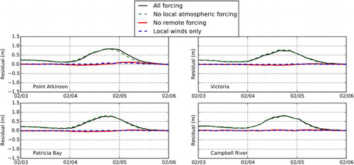
Fig. 6 Modelled residuals (solid line) compared with a simulation of the surge propagation without tidal forcing (dashed line) for the February 2006 hindcast.

First, it is clear that remote forcing at the open boundary contributes most significantly to the surge at each of these locations (Fig. 5). When the remote forcing is not included as a forcing condition, the surge drops from a maximum of 84 cm to 11 cm at Point Atkinson and its maximum occurs eight hours later. A similar drop in the maximum surge and delay in timing of the maximum surge is observed at the other locations. When local atmospheric forcing is neglected, almost all the surge amplitude is accounted for in the remote forcing.

The contribution to the surge due to local atmospheric forcing is small and appears to be geographically dependent, most likely a result of the effects of the local winds. Removal of the local atmospheric forcing leads to a drop of about 2 cm in the maximum surge at Point Atkinson and 2.5 cm at Campbell River. By contrast, the surge amplitude increases by 4.5 cm at Victoria and 3.6 cm at Patricia Bay. The southeasterly winds over the Strait of Georgia could be acting to push water away from the southern tip of Vancouver Island, resulting in a slight decrease in the surge amplitude at Victoria and Patricia Bay when wind effects are included in the model. A simulation with only tides and local wind forcing produces a surge of 7.8 cm at Point Atkinson, a small fraction of the total observed surge, and only centimetres at the other locations. Note that this wind-induced surge occurs well after the peak surge occurred in both the observations and simulations with full forcing.

A simple steady state argument balancing the wind stress with the pressure gradient can be used to calculate the slope of the sea surface in a body of water with a constant depth (Pugh, 2004):(6) where is the coefficient of friction, is the density of air, is the acceleration due to gravity, is the wind speed, and is the density of water. Assuming , kg m⁻³, kg m⁻³, wind speed m s⁻¹, and depth m, the slope of the sea surface is approximately . At Point Atkinson, a westerly wind can act over a small distance of approximately 50 km, giving a sea surface elevation on the order of centimetres in agreement with the model findings. Because the Strait of Georgia is not a constant depth and is up to 400 m deep, this calculation is only an approximation. Choosing a larger depth would result in an even smaller estimate for the sea surface elevation caused by wind stresses. Further, northwesterly winds would induce the largest elevations at Point Atkinson because of the large distance over which the winds can act.

Next, the surge amplitude decreases by a few centimetres at all four locations if local atmospheric pressure is not included in the surface forcing. This drop is smaller than the IB sea level change calculated by Eq. (1), an approximately 1 cm rise in sea level associated with a 1 hPa drop in atmospheric pressure. In this event, the pressure at Vancouver International Airport dropped to about 99,000 Pa (Environment Canada, 2014a), corresponding to a 20 cm rise in sea level. This magnitude is in line with the findings of Murty et al. (1995) that the IB contributes up to one-third of the total surge amplitude. In our model, realistic surge amplitudes are produced by including the influence of atmospheric pressure forcing in the sea level at the open boundary. This indicates that the IB response of sea level to atmospheric pressure variation is mostly accounted for. If the IB response at the boundary is set to zero (by excluding the remote forcing), and the local atmospheric pressure variation is included, the model obtains a much smaller response to atmospheric pressure forcing. This suggests that the local atmospheric pressure variation must be combined with the remote variation to generate the full IB response in the Salish Sea.

These comparisons point to the importance of including the surge entering the domain from the Pacific Ocean as a forcing condition at the open boundary. Storms travelling over the Pacific Ocean towards the west coast of the northern United States and Canada can induce elevated sea levels along the coastline which then enter the Salish Sea system through Juan de Fuca Strait. Previous simulations by Murty et al. (1995) suggest that surges entering the system through the Strait of Juan de Fuca contribute most significantly to storm surges in this domain. The result of our study is consistent with these findings.

Next, an assessment of the importance of including the tide–surge interaction, which is important in shallow regions because of non-linear effects and bottom friction (Bernier & Thompson, 2007), is presented for this hindcast (Fig. 6). The most significant differences occur at Point Atkinson where the maximum of the surge-only case is 8.4 cm higher than the maximum modelled residual, about 10% of the total surge amplitude. In contrast, the tide–surge interaction at Victoria is hardly noticeable. Indeed, a spatial map of the difference between the modelled residual and the surge-only simulation (Fig. 7) indicates that the tide–surge interaction is more pronounced north of the San Juan and Gulf islands. The passages between these islands are known for vigorous tidal mixing, which may have a non-linear effect on surge propagation. However, the effect is a relatively small overestimate of the surge elevation, and there are no changes in the timing of the surge. So, in operational settings, performing a surge-only simulation and adding the predicted tides a posteriori could be more computationally efficient with only a small decrease in the accuracy of the prediction.

Fig. 7 Spatial dependency of tide–surge interaction in the February 2006 hindcast. Differences in sea surface height between simulations with tidal forcing and without tidal forcing. Each plot is an average over 4 hr.

c Spatial Extent of Surge

A major wind storm on 15 December 2006 is hindcast next. Although the storm was very strong (gusts over 120 km hr⁻¹) and the observed residual at Point Atkinson reached 94 cm, this event did not coincide with high tide, so no significant or reported flooding occurred in the Vancouver area (Forseth, 2012). Because of the high winds, this event has been used to examine the propagation of the surge throughout the domain and spatial variations in the surge amplitude. First, an assessment of the accuracy of the hindcast is provided.

Modelled residuals are generally too low in this hindcast (Fig. 8); however, the timing of the surge agrees well. All Willmott skill scores rank above 0.89 and the measure also indicates good agreement between model and observations (Table 2). The measure suggests that the standard deviation of the error in the modelled residuals is roughly half the standard deviation of the observed residuals. Note that the performance has degraded when compared with the February 2006 and November 2006 cases. This could be due to a number of factors. First, the very high wind speeds observed during this storm are significantly underrepresented by the atmospheric model leading to lower wind stress and less piling of water against the coast. Second, the anomaly forcing at the open boundaries could be too low. The observed residual at Tofino, British Columbia (a point near to but outside the domain) is up to 10 cm lower than the observed residual at Neah Bay, Washington (a point inside the domain, near the boundary). Because the storm surge is less sensitive to wind forcing than anomaly forcing at the open boundaries, the latter is likely the cause although it still does not account for all the error.

Fig. 8 Comparison of observed and modelled water level and residuals during the 15 December 2006 storm surge simulation.

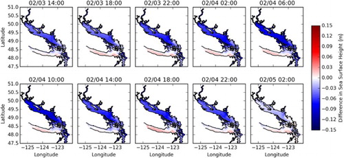
The evolution and spatial distribution of the surge is highlighted in Fig. 9 in which the modelled residual is plotted every hour beginning at 0230 UTC 15 December to 1130 UTC 15 December. The surge enters the system from Juan de Fuca Strait, peaking between 0930 UTC 15 December and 1130 UTC 15 December then begins to subside throughout the entire domain. Notably, the Strait of Georgia experiences the largest surge values, approximately 70 cm, whereas the Juan de Fuca region experiences a maximum surge around 60 cm (Fig. 9). Additionally, the coastal areas on the mainland side of the Strait of Georgia experience slightly higher surges (∼10 cm) than the Vancouver Island side, likely because of the southerly wind in the atmospheric model pushing water against the mainland coast. At about 1130 UTC, the winds at Point Atkinson switch to northwesterly then westerly, further amplifying the surge along the mainland coast.

Fig. 9 Propagation of the storm surge on 15 December 2006. Modelled residual every hour starting at 0230 UTC 15 December. Time advances from top left to bottom right. Wind vectors from the atmospheric forcing are overlaid in black.

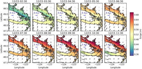
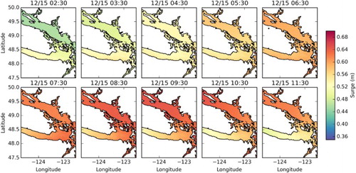
In a simulation without atmospheric forcing, the surge amplitude across the Strait of Georgia is uniform with no pronounced difference between the mainland side and the Vancouver Island side (Fig. 10). Although the surge entering the domain from the Pacific Ocean is the leading order contribution, the winds may induce localized changes to the surge amplitude. Interestingly, the winds over Juan de Fuca Strait cause a decrease in surge amplitude in this region because the winds are acting to push the water towards the mainland (Fig. 9). Even without atmospheric forcing, there is still a significant difference in surge amplitude between the Strait of Georgia and Juan de Fuca Strait, perhaps because the incoming surge wave could be partially reflected from the mainland coast in the Strait of Georgia. Because local winds are stronger in this case, their contribution to the surge amplitude of about 6 cm at Point Atkinson is more significant than in the February 2006 case. However, this is still less than 10% of the total surge amplitude.

Fig. 10 As in Fig. 9, but for a simulation that does not include atmospheric forcing.

d Strong Wind Event

Next, a relatively strong wind event recorded at Point Atkinson on 19 November 2009 is considered. Wind speeds at Point Atkinson reached 18 m s⁻¹, which is approximately the same magnitude as that observed on 4 February 2006. Although high wind speeds were observed, the surge associated with this event is rather small compared with the previous cases (Fig. 11). Two significant surge events are noted, the first occurring on 19 November with an observed amplitude of about 55 cm at Point Atkinson and a second, larger surge of 70 cm on 20 November. The strong wind event of 19 November was associated with the smaller of the two surges, supporting the fact that local winds do not contribute significantly to surge amplitudes. Neither of the surges occurred during a high tide, so no high water level events were recorded. Although the sea surface height plots are not shown here, a maximum surge was also observed at the other three locations on 20 November, which appears to be linked to a secondary high wind event and another surge entering the system at Tofino and Port Hardy.

Fig. 11 Wind and storm surge conditions at Point Atkinson for a strong wind event on 19 November 2009. (top) Wind speed from Environment Canada observations (Environment Canada, 2014a) at Point Atkinson (solid line) and from the atmospheric model (CGRF) at a grid point near Point Atkinson (dashed line). (middle) Sea surface height anomaly at Tofino (solid line) and Port Hardy (dashed line) used as forcing conditions at the western and northern open boundaries. (bottom) Observed (solid line) and modelled (dashed line) residuals at Point Atkinson.

Danard et al. (2003) discuss the role of wind fetch, the distance over which wind acts on the surface of a water basin, in setting up seiche motion in lakes and its contribution to storm surges. As wind blows over the surface of a lake, the water level becomes elevated on the downwind side and depressed on the upwind side in response to wind-induced currents. The longer the fetch, the more significant the tilting of the water surface. These changes in water level can also contribute to storm surges. During the high wind events on 19 and 20 November, the winds at Point Atkinson were directed to the west, explaining the lack of strong surge observed during this event because wind stresses would act to depress the water on the east side of the basin. In fact, the surge amplitude at Victoria on 20 November was 71.8 cm which is slightly higher than that observed at Point Atkinson (70 cm). Of the cases considered so far, this is the only example in which the surge amplitude at Victoria was higher than that at Point Atkinson. The model results do not reflect a higher surge at Victoria (54 cm versus 58.7 cm at Point Atkinson), perhaps because of an underestimate in the wind speed and some discrepancies in the wind direction of the atmospheric forcing. There is a fairly significant delay in the timing of the maximum surge at most stations (Table 3). The model's surge curve is much broader and does not contain the narrow peak on 20 November as seen in the observations. Both the observations and remote forcing contain a relatively fast rise in the surge curve that is not reproduced in the model, which might be explained by errors in the model wind speed and direction.

The modelled water levels and residuals are, on average, too high for this hindcast, except at Victoria (Table 2). Generally, the skill scores are very good, scoring above 0.89 at all stations.

e High-Resolution Atmospheric Forcing

The above comparison between modelled and observed winds at Point Atkinson suggests that the atmospheric forcing product (CGRF) may not be adequate to produce accurate storm surge hindcasts because the wind speeds are substantially lower than observed. The CGRF is a global atmospheric reforecasting model with a horizontal resolution of approximately 33 km over the Salish Sea domain, which is problematic because the Strait of Georgia itself is only about 30 km wide. As such, there are only one or two grid cells that are entirely over water in our domain, resulting in overly damped wind speeds at grid points close to land like Point Atkinson. To determine the effect of under-resolved wind forcing on the storm surge hindcasts we compare simulations that have been forced with (i) the low-resolution CGRF model and (ii) a high-resolution (2.5 km) HRDPS model from Environment Canada. These simulations are performed for a storm surge that occurred on 17 December 2012 and cover the time period 14–19 December 2012. The high-resolution product is not available for the hindcasts already discussed.

First, a comparison of the wind speed and direction for the two models and observations is provided in Fig. 12 at Point Atkinson, Sandheads, and a National Oceanic and Atmospheric Administration (NOAA) buoy at Neah Bay. Sandheads is a lighthouse station in the southern Strait of Georgia. For each of the models, the wind speed and direction towards which the wind is heading, at the closest grid point to the longitude and latitude of Point Atkinson, Sandheads, and the NOAA buoy, is used for comparison. Although the low-resolution CGRF model has a grid spacing of 33 km, grid points align closely with these locations. At Point Atkinson, the high-resolution model is in very good agreement with observations for both the wind speed and direction; however, the low-resolution CGRF model significantly underestimates the wind speed during high wind periods on 15 December 2012 and 17 December 2012. At Sandheads, both the low-resolution and high-resolution models agree well with observations. The low-resolution model simulates the wind speed well at Sandheads, likely because this grid cell happens to be mostly over water. Although not shown here, both models have a similar sea level atmospheric pressure at these locations. Note that data assimilation is used in the parent model of the nested HRDPS product.

Fig. 12 Comparison of observed and modelled winds during the December 2012 storm surge simulation at (top) Point Atkinson, (middle) Sandheads, and (bottom) NOAA Buoy 46087. Observed winds are shown in solid black, low-resolution CGRF model in dashed black, and high-resolution model in grey. Observations from Sandheads and Point Atkinson are from the Environment Canada Climate Data archives (Environment Canada, 2014a). Observations at the NOAA Buoy were downloaded from http://www.ndbc.noaa.gov/stationpage.php?station=46087. Wind direction represents the direction that the wind is headed.

Hindcasts with both atmospheric forcing products agree well with observations (Fig. 13). Willmott skill scores for both modelled residuals are above 0.84 at these four locations. There is considerable noise in the observed Campbell River residual, which could explain its low skill score (Table 2). The modelled residuals in each simulation deviate only slightly from each other, most noticeably at Point Atkinson during the strong wind event on 15 December 2012 when the simulation with the low-resolution atmospheric forcing has a residual that is 5 cm higher. The maximum residuals on 17 December 2012 are almost identical at each station (Table 3). Although the wind speeds on 15 December 2012 are quite high, this event did not result in any flooding or residuals greater than 50 cm. Significant flooding occurred later, on 17 December 2012, when the observed surge amplitude at Point Atkinson was 66.3 cm. Even though the low-resolution model significantly underpredicts the wind speed at some locations, it performs comparably to forcing with high-resolution products. Much of the fine-scale detail offered by the high-resolution atmospheric model is averaged out because, to first order, the storm surge is a spatial integral of the wind. This result further demonstrates that the local wind is not the most important factor in setting up storm surges over this domain; however, local wind patterns contribute to wave conditions that can impact flooding and are not accounted for in this model.

Fig. 13 Comparison of observed (solid black line) and modelled residuals for the December 2012 storm surge simulation. Modelled residuals from two simulations using low-resolution (dashed line) and high-resolution (grey line) atmospheric products are shown.

5 Conclusions and discussion

In this article, we describe a three-dimensional numerical ocean model of the Salish Sea for accurate hindcasts of storm surges in the Strait of Georgia. The model is forced with eight tidal constituents at the western and northern open boundaries, as well as the sea surface height anomaly from de-tided observations at Tofino and Port Hardy. Additionally, wind stress and local atmospheric pressure forcing were used at the ocean surface using an atmospheric reforecasting product called CGRF (Smith et al., 2014). Storm surge simulations began with zero initial conditions for the currents and sea surface height and were started several days prior to the event of interest to spin up the velocity fields.

Hindcasts of five significant events in February 2006, November 2006, December 2006, November 2009, and December 2012 were simulated. In general, the model performs well in reproducing the observed water level heights and residuals, with Willmott skill scores greater than 0.84 in all cases and generally higher skill scores for the water level heights. Further, in a single simulation, the skill scores are fairly consistent among the four stations examined. We have also assessed the relative importance of different forcing factors contributing to the storm surge. The sea surface height anomaly entering the system from the Pacific Ocean, or remote forcing, contributes most significantly to the surge amplitude, in agreement with previous studies in this region (Murty et al., 1995). Although the large-scale wind patterns and atmospheric conditions are important in setting up the surge on the Pacific Ocean boundaries, the local winds within the Strait of Georgia are not the leading order contribution to surge amplitude. However, the local wind patterns can set up small spatial differences in the surge, resulting in higher surges on the mainland side of the Strait of Georgia because of the usually southerly winds during storm surge season. Additionally, surge amplitudes in the Strait of Georgia are typically higher than those in Juan de Fuca Strait, perhaps because of a partial reflection of the surge from the mainland coast. Results from an additional simulation with no tidal forcing but only surge propagation and atmospheric forcing found that non-linear effects resulting from the tide–surge interaction were most important north of the San Juan and Gulf Islands. The modelled surge amplitude increased by about 10% at Point Atkinson when the tide-surge interaction was neglected in one example.

Comparisons between high-resolution and low-resolution atmospheric forcing further suggest that local winds are not the leading order factor in setting up large surge amplitudes. The low-resolution model significantly underestimated wind speeds in certain areas of the domain; however, it performed just as accurately as the high-resolution product in reproducing surge amplitudes. Although the high-resolution model delivers fine-scale detail and more accurate local wind patterns, it did not improve on the surge hindcast. Because both of these products provide the same level of accuracy for storm surge hindcasts, in the future we will use the high-resolution atmospheric model to produce real-time storm surge predictions, even though most of the testing was performed with the low-resolution model. Additionally, the sea surface height anomaly boundary condition of the present model will be taken from the solution of a large-scale forecasting model.

Several factors considered in other storm surge modelling studies have been neglected in these simulations. Primarily, effects due to wetting and drying have not been included. These are an important factors to consider in shallow, low-lying areas where water levels retreat significantly to reveal land. In this article, the four locations used to assess storm surge accuracy are not in shallow regions, so wetting and drying are not considered important. However, several communities in the Strait of Georgia, such as Boundary Bay and Crescent Beach, are in shallow regions and are typically most affected by storm surge during winter. As such, efforts to include wetting and drying will be considered in the future. Additionally, flooding effects resulting from wave run up are left for a more detailed inundation study with higher resolution in the near-shore areas. Local winds have a significant effect on wave action, which is a primary concern for flooding management. Further, the remote forcing is applied uniformly across the open boundary, so any spatial variability in the incoming surge is not accounted for in the model. Because remote forcing is an important contributing factor, any forecasting with this regional model must make use of results from a larger-scale prediction system.

Because the Strait of Georgia is a large, semi-enclosed body of water, storm surges can behave and evolve differently than in other coastal regions. For instance, the complicated coastlines and local wind patterns result in important spatial variations in the surge amplitude. As such, the strong wind caused by a large storm is not the only factor to be considered in community preparedness for surge conditions. The geometry of the Strait and local wind patterns render communities on the mainland side of the southern Strait of Georgia more susceptible to surges. Additionally, communities such as Campbell River are at risk because of the long fetch and predominately southerly winds during the winter months.

Finally, difficulties in reproducing accurate M₂ tidal harmonics in both the Strait of Georgia and Juan de Fuca Strait have been highlighted in this study among others (Foreman et al., 2004; Stronach et al., 1993). Future work will attempt to improve model accuracy by examining mixing parametrizations and energy dissipation resulting from bottom friction and their effect on tidal harmonics and by investigating stratified effects on surge amplitudes. Additionally, a biological-chemical modelling component will be added.

Acknowledgements

We would like to thank Michael Foreman, Diane Masson, Luc Fillion, Rich Pawlowicz, Mark Halverson, Kao-Shen Chung, and Pramod Thupaki for providing data used in the model set-up and evaluation. For providing guidance with stakeholder engagement, we also thank Stephanie Chang, Jackie Yip, and Shona van Zijil de Jong. This research was enabled in part by support provided by WestGrid (www.westgrid.ca) and Compute Canada Calcul Canada (www.computecanada.ca).

Disclosure statement

No potential conflict of interest was reported by the authors.

ORCID

Nancy Soontiens http://orcid.org/0000-0003-2880-8717

Additional information

Funding

This project is funded by the Marine Environmental Observation Prediction and Response Network (MEOPAR), a Network of Centres of Excellence of Canada.

Appendix A: Details on tidal tuning

This appendix details the procedure used to tune the tidal forcing for a good match with observations in the Strait of Georgia. Originally, the eight most important tidal constituents were extracted from a tide prediction tool called Webtide (Webtide, 2014) at the western boundary of Juan de Fuca Strait based on work by Foreman et al. (2000). At the northern boundary, M₂ and K₁ tidal harmonics for both elevation and currents were taken from Thomson and Huggett (1980), as well as elevation harmonics for O₁ and S₂. The remaining constituents were extrapolated from Webtide based on the ratio between S₂ and M₂ amplitudes and phase differences for the semi-diurnal constituents and O₁ and K₁ for the diurnal constituents. However, these forcing conditions did not result in a good match between observed and modelled tidal elevation harmonics in the Strait of Georgia, the main region of interest (although the matches in Juan de Fuca Strait were adequate). As such, tidal forcing was tuned by first adjusting the western boundary M₂ and K₁ phase and K₁ amplitude for a good match in the Strait of Georgia (specifically at Point Atkinson, Gibsons Landing, Winchelsea, and Halfmoon Bay). This tuning was performed on simulations that used only M₂ and K₁ forcing. Next, the M₂ and K₁ fluxes at the northern boundary were adjusted because the cross-sectional area of the transect used by Thomson and Huggett (1980) to measure tidal currents in Johnstone Strait is smaller than the cross-sectional area of our northern boundary. The northern boundary tides were tuned for good matches at Yorke Island and Kelsey Bay. Finally, the remaining constituents were added, starting with O₁, then S₂, then in pairs P₁/N₂ and Q₁/K₂. Final adjustments were made by varying amplitude and phase slightly, evaluating the changes to M₂, K₁ and the ratios S₂:M₂, N₂:M₂, K₂:M₂, O₁:K₁, P₁:K₁, Q₁:K₁, then choosing new values to move closer to the observations by linear interpolation.

Table A1 compares the M₂ and K₁ elevation harmonics with data from Foreman et al. (1995), Foreman et al. (2004), and Foreman et al. (2012). Overall, the average complex difference for M₂ is 8.05 cm and for K₁ is 2.58 cm, but both constituents perform very well in the Strait of Georgia region.

Table A1. Comparisons of modelled and observed amplitudes and phases. R is the ratio of modelled to observed amplitude. Δϕ is the difference between modelled and observed phase. D is the amplitude of the complex difference. The mean error and root mean square (RMS) error are calculated as the difference between the modelled quantity and observed quantity.

				M2			K1
	Station name	Longitude	Latitude		(deg)	(cm)		(deg)	(cm)
1	Port Renfrew	−124.43	48.55	1.16	−9.40	16.63	1.03	−4.94	4.17
2	Sheringham Point	−123.92	48.38	1.19	−16.47	17.95	1.00	−4.44	4.24
3	Pedder Bay	−123.55	48.33	0.96	−27.39	15.91	0.99	−2.41	2.66
4	Esquimalt	−123.43	48.43	0.91	−23.09	14.40	0.99	−1.04	1.21
5	Victoria	−123.37	48.42	0.89	−17.77	11.62	1.04	−1.83	3.22
6	Clover Point	−123.35	48.41	0.83	−17.95	13.39	1.03	−2.23	3.14
7	Finnerty Cove	−123.30	48.47	0.83	−8.24	9.47	1.02	−2.19	3.25
8	Fulford Harbour	−123.45	48.77	0.82	−3.08	10.78	1.00	−0.63	0.83
9	Tumbo Channel	−123.11	48.79	1.05	2.03	4.43	1.04	0.66	3.34
10	Patos Island	−122.97	48.78	1.03	0.26	2.32	1.04	−1.50	3.92
11	Whaler Bay	−123.33	48.89	1.00	−0.76	1.10	1.01	−0.48	1.19
12	Tsawwassen	−123.13	48.99	1.00	0.92	1.31	1.01	0.19	1.09
13	Sandheads	−123.30	49.10	1.02	−1.05	2.58	1.04	−0.59	3.15
14	Point Grey	−123.27	49.25	0.98	−3.31	5.83	0.96	−0.68	3.63
15	Point Atkinson	−123.25	49.33	1.01	−0.48	1.07	1.00	−0.56	0.94
16	Gibsons Landing	−123.50	49.40	0.98	0.75	2.34	1.00	0.96	1.47
17	Winchelsea	−124.08	49.30	1.01	−0.19	0.78	1.01	0.51	1.30
18	Halfmoon Bay	−123.92	49.52	1.01	−0.15	0.83	1.01	0.15	0.72
19	Irvines Landing	−124.05	49.63	1.00	−0.32	0.59	1.01	0.24	1.12
20	Powell River	−124.55	49.86	1.00	−1.72	3.05	1.00	−0.01	0.43
21	Little River	−124.92	49.74	1.03	0.07	2.54	1.01	0.33	0.73
22	Lund	−124.76	49.98	1.02	−2.52	4.98	1.02	−0.95	2.45
23	Twin Islets	−124.93	50.03	1.02	−2.05	4.22	1.01	−0.24	0.72
24	Campbell River	−125.24	50.04	0.99	0.51	1.12	1.00	0.94	1.39
25	Maude Island E	−125.33	50.13	1.13	−10.02	12.62	0.97	−1.44	2.89
26	Nymphe Cove	−125.36	50.13	1.02	−5.43	6.04	0.97	−0.29	2.02
27	Seymour Narrows	−125.34	50.13	0.63	31.31	53.40	1.14	10.91	17.28
28	Brown Bay	−125.37	50.16	0.98	−5.63	9.26	0.98	−0.04	1.17
29	Chatham Point	−125.44	50.33	1.09	−5.49	12.18	0.98	−3.18	3.85
30	Kelsey Bay	−125.96	50.39	1.00	−1.69	3.50	0.98	−0.39	1.00
31	Yorke Island	−125.97	50.44	0.99	1.59	3.32	1.01	1.23	1.37
	Mean Error			4.23 (cm)	6.50	8.05	1.56 (cm)	1.49	2.58
	RMS Error			7.67 (cm)	10.73	12.73	2.41 (cm)	2.57	3.91

The underlying research materials for this article can be accessed at https://bitbucket.org/salishsea/storm-surge, which contains analysis scripts and situation description files.

References

- Abeysirigunawardena, D. S., Smith, D. J., & Taylor, B. (2011). Extreme sea surge responses to climate variability in coastal British Columbia, Canada. Annals of the Association of American Geographers, 101(5), 992–1010. doi: 10.1080/00045608.2011.585929
- Bernier, N., & Thompson, K. (2006). Predicting the frequency of storm surges and extreme sea levels in the northwest Atlantic. Journal of Geophysical Research: Oceans, 111, C10009. doi: 10.1029/2005JC003168
- Bernier, N., & Thompson, K. (2007). Tide-surge interaction off the east coast of Canada and northeastern United States. Journal of Geophysical Research: Oceans, 112, C06008. doi: 10.1029/2006JC003793
- Bernier, N., & Thompson, K. (2010). Tide and surge energy budgets for eastern Canadian and northeast US waters. Continental Shelf Research, 30(3), 353–364. doi: 10.1016/j.csr.2009.12.003
- Bobanović, J., Thompson, K. R., Desjardins, S., & Ritchie, H. (2006). Forecasting storm surges along the east coast of Canada and the north-eastern United States: The storm of 21 January 2000. Atmosphere-Ocean, 44(2), 151–161. doi: 10.3137/ao.440203
- Brossier, C. L., Béranger, K., & Drobinski, P. (2012). Sensitivity of the northwestern Mediterranean Sea coastal and thermohaline circulations simulated by the 1/12-resolution ocean model NEMO-MED12 to the spatial and temporal resolution of atmospheric forcing. Ocean Modelling, 43-44, 94–107. doi: 10.1016/j.ocemod.2011.12.007
- Crean, P., Murty, T. S., & Stronach, J. (1988). Mathematical modelling of tides and estuarine circulation: The coastal seas of southern British Columbia and Washington state (Vol. 30). New York: American Geophysical Union.
- Crean, P. B., Murty, T. S., & Stronach, J. A. (1988). Numerical-simulation of oceanographic processes in the waters between Vancouver Island and the mainland. Oceanography and Marine Biology, 26, 11–142.
- Danard, M., Munro, A., & Murty, T. (2003). Storm surge hazard in Canada. Natural Hazards, 28(2–3), 407–434. doi: 10.1023/A:1022990310410
- de Young, B., Lu, Y., & Greatbatch, R. (1995). Synoptic bottom pressure variability on the Labrador and Newfoundland continental shelves. Journal of Geophysical Research, 100(C5), 8639–8653. doi: 10.1029/95JC00231
- Engedahl, H. (1995). Use of the flow relaxation scheme in a three-dimensional baroclinic ocean model with realistic topography. Tellus A, 47(3), 365–382. doi: 10.1034/j.1600-0870.1995.t01-2-00006.x
- Environment Canada. (2014a). Climate database. Retrieved from http://climate.weather.gc.ca/indexe.html
- Environment Canada. (2014b). High resolution deterministic prediction system. Retrieved from https://weather.gc.ca/grib/grib2HRDPSHRe.html
- Fisheries and Oceans Canada. (2014). Canadian tides and water level data archive. Retrieved from http://www.isdm-gdsi.gc.ca/isdm-gdsi/twl-mne/index-eng.htm
- Flather, R. A. (1994). A storm surge prediction model for the northern Bay of Bengal with application to the cyclone disaster in April 1991. Journal of Physical Oceanography, 24(1), 172–190. doi: 10.1175/1520-0485(1994)024<0172:ASSPMF>2.0.CO;2
- Foreman, M., Crawford, W., Cherniawsky, J., Henry, R., & Tarbotto, M. (2000). A high-resolution assimilating tidal model for the northeast Pacific Ocean. Journal of Geophysical Research, 105(C1), 28,629–28,652. doi: 10.1029/1999JC000122
- Foreman, M., Stucchi, D., Garver, K., Tuele, D., Isaac, J., Grime, T., … Morrison, J. (2012). A circulation model for the Discovery Islands, British Columbia. Atmosphere-Ocean, 50(3), 301–316. doi: 10.1080/07055900.2012.686900
- Foreman, M., Sutherland, G., & Cummins, P. (2004). M2 tidal dissipation around Vancouver Island: An inverse approach. Continental Shelf Research, 24(18), 2167–2185. doi: 10.1016/j.csr.2004.07.008
- Foreman, M., Walters, R., Henry, R., Keller, C., & Dolling, A. (1995). A tidal model for eastern Juan de Fuca Strait and the southern Strait of Georgia. Journal of Geophysical Research, 100(C1), 721–740. doi: 10.1029/94JC02721
- Forseth, P. (2012). Adaptation to sea level rise in metro Vancouver: A review of literature for historical sea level flooding and projected sea level rise in metro Vancouver (Tech. Rep.). Simon Fraser University.
- Giddings, S., MacCready, P., Hickey, B., Banas, N., Davis, K., Siedlecki, S., … Connolly, T. (2014). Hindcasts of potential harmful algal bloom transport pathways on the Pacific Northwest coast. Journal of Geophysical Research: Oceans, 119(4), 2439–2461.
- Gray, M., Danard, M., Flather, R., Henry, F., Murty, T., Venkatesh, S., & Jarvis, C. (1984). A preliminary investigation using a Nova Scotia storm surge prediction model. Atmosphere-Ocean, 22(2), 207–225. doi: 10.1080/07055900.1984.9649194
- Haugerud, R. A. (1999). Digital elevation model (DEM) of Cascadia, latitude 39N-53N, longitude 116W-133W. U. S. Geological Survey Open-File Report 99-369. Retrieved from http://pubs.usgs.gov/of/1999/0369/
- Holton, J. (1992). An introduction to dynamic meteorology. San Diego, California: Academic Press.
- Hubbert, G. D., & McInnes, K. L. (1999). A storm surge inundation model for coastal planning and impact studies. Journal of Coastal Research, 15(1), 168–185.
- Lane, E. M., & Walters, R. A. (2009). Verification of RICOM for storm surge forecasting. Marine Geodesy, 32(2), 118–132. doi: 10.1080/01490410902869227
- Ma, Z., Han, G., & de Young, B. (2015). Oceanic responses to Hurricane Igor over the Grand Banks: A modeling study. Journal of Geophysical Research: Oceans, 120. doi: 10.1002/2014JC010322
- Madec, G. (2012). NEMO ocean engine. Note du Pôle de modélisation de l'Institut Pierre-Simon Laplace No. 27, France.
- Maraldi, C., Chanut, J., Levier, B., Ayoub, N., De Mey, P., Reffray, G., … Marsaleix, P., and the Mercator Research and Development Team. (2013). NEMO on the shelf: Assessment of the Iberia-Biscay-Ireland configuration. Ocean Science, 9, 745–771. doi: 10.5194/os-9-745-2013
- Masson, D., & Cummins, P. F. (2004). Observations and modeling of seasonal variability in the Straits of Georgia and Juan de Fuca. Journal of Marine Research, 62(4), 491–516. doi: 10.1357/0022240041850075
- Masson, D., & Fine, I. (2012). Modeling seasonal to interannual ocean variability of coastal British Columbia. Journal of Geophysical Research, 117, C10019. doi: 10.1029/2012JC008151
- Mercer, D., Sheng, J., Greatbatch, R. J., & Bobanović, J. (2002). Barotropic waves generated by storms moving rapidly over shallow water. Journal of Geophysical Research: Oceans, 107(C10), 3152, doi: 10.1029/2001JC001140
- Morrison, J., Foreman, M., & Masson, D. (2011). A method for estimating monthly freshwater discharge affecting British Columbia coastal waters. Atmosphere-Ocean, 50(1), 1–8. doi: 10.1080/07055900.2011.637667
- Murty, T., Venkatesh, S., Danard, M., & El-Sabh, M. (1995). Storm surges in Canadian waters. Atmosphere-Ocean, 33(2), 359–387. doi: 10.1080/07055900.1995.9649537
- Parker, B. B. (2007). Tidal analysis and prediction (Tech. Rep.). NOAA Special Publication NOS CO-OPS 3. Silver Spring, Maryland: NOAA.
- Pawlowicz, R., Beardsley, B., & Lentz, S. (2002). Classical tidal harmonic analysis including error estimates in MATLAB using T TIDE. Computers & Geosciences, 28(8), 929–937. doi: 10.1016/S0098-3004(02)00013-4
- Pawlowicz, R., Riche, O., & Halverson, M. (2007). The circulation and residence time of the Strait of Georgia using a simple mixing-box approach. Atmosphere-Ocean, 45, 173–193. doi: 10.3137/ao.450401
- Pugh, D. (2004). Changing sea levels: Effects of tides, weather and climate. Cambridge, UK: Cambridge University Press.
- Smith, G. C., Roy, F., Mann, P., Dupont, F., Brasnett, B., Lemieux, J.-F., … Bélair, S. (2014). A new atmospheric dataset for forcing ice–ocean models: Evaluation of reforecasts using the Canadian global deterministic prediction system. Quarterly Journal of the Royal Meteorological Society, 140(680), 881–894. doi: 10.1002/qj.2194
- Stronach, J., Backhaus, J., & Murty, T. (1993). An update on the numerical simulation of oceanographic processes in the waters between Vancouver Island and the mainland: The GF8 model. Oceanography and Marine Biology: An Annual Review, 31, 1–86.
- Strub, P., & James, C. (2002). Altimeter-derived surface circulation in the large-scale NE Pacific Gyres.: Part 2: 1997–1998 El Niño anomalies. Progress in Oceanography, 53(2), 185–214. doi: 10.1016/S0079-6611(02)00030-7
- Sutherland, D. A., MacCready, P., Banas, N. S., & Smedstad, L. F. (2011). A model study of the Salish Sea estuarine circulation. Journal of Physical Oceanography, 41(6), 1125–1143. doi: 10.1175/2011JPO4540.1
- Thompson, K. R., Sheng, J., Smith, P. C., & Cong, L. (2003). Prediction of surface currents and drifter trajectories on the inner Scotian Shelf. Journal of Geophysical Research, 108(C9), 3287. doi: 10.1029/2001JC001119
- Thomson, R. E. (1981). Oceanography of the British Columbia coast (Vol. 56). Department of Fisheries and Oceans: Sidney, BC.
- Thomson, R. E., & Huggett, W. S. (1980). M2 baroclinic tides in Johnstone Strait, British Columbia. Journal of Physical Oceanography, 10, 1509–1539. doi: 10.1175/1520-0485(1980)010<1509:MBTIJS>2.0.CO;2
- Tinis, S. (2014). BC Storm Surge Forecasting Program. Retrieved from http://stormsurgebc.ca
- Umlauf, L., & Burchard, H. (2003). A generic length-scale equation for geophysical turbulence models. Journal of Marine Research, 61(2), 235–265. doi: 10.1357/002224003322005087
- Webtide. (2014). WebTide tidal prediction model. Retrieved from http://www.bio.gc.ca/science/researchrecherche/ocean/webtide/index-en.php
- Weisberg, R. H., & Zheng, L. (2006). Hurricane storm surge simulations for Tampa Bay. Estuaries and Coasts, 29(6), 899–913. doi: 10.1007/BF02798649
- Willmott, C. J. (1982). Some comments on the evaluation of model performance. Bulletin of the American Meteorological Society, 63(11), 1309–1313. doi: 10.1175/1520-0477(1982)063<1309:SCOTEO>2.0.CO;2
- Wright, D. G., Greenberg, D. A., & Majaess, F. G. (1987). The influence of bays on adjusted sea level over adjacent shelves with application to the Labrador Shelf. Journal of Geophysical Research, 92(C13), 14610–14620. doi: 10.1029/JC092iC13p14610
- Xu, H., Zhang, K., Shen, J., & Li, Y. (2010). Storm surge simulation along the US East and Gulf Coasts using a multi-scale numerical model approach. Ocean Dynamics, 60(6), 1597–1619. doi: 10.1007/s10236-010-0321-3