Performance of One-Way and Two-Way Nesting Techniques Using the Shelf Circulation Modelling System for the Eastern Canadian Shelf

Abstract

The performance of one-way and two-way nesting techniques is assessed in this study using model results produced by a regional ocean circulation modelling system for the eastern Canadian shelf. The assessment is made in terms of dynamical consistency between the parent model (PM) and child model (CM), representation of general circulation features, and reduction of numerical noise generated during the interaction of the PM and CM. It is demonstrated that the feedback from the CM to the PM in numerical experiments using two-way nesting ensures that the large-scale circulation produced by the PM and CM be dynamically consistent over the region where the two model domains overlap. In comparison with one-way nesting, two-way nesting leads to a better representation of coastal currents over the Gulf of St. Lawrence and the Scotian Shelf and improves the large-scale circulation in the results produced by the PM. This study also examines an alternative two-way nesting technique based on the semi-prognostic method in which differences between the PM and CM densities are used to adjust the horizontal momentum balance in the PM. Model results demonstrate the advantage of the semi-prognostic method in eliminating numerical noise during the feedback from the CM to PM while ensuring dynamical consistency between the two model components.

Résumé

[Traduit par la rédaction] Nous examinons l'effet de techniques unidirectionnelles et bidirectionnelles d'imbrication, à l'aide de résultats de modèles provenant d'un système régional de modélisation de la circulation océanique, pour le plateau est du Canada. L’évaluation porte sur la cohérence dynamique entre les modèles parent (PM) et enfant (CM), la représentation de caractéristiques générales de la circulation et la réduction du bruit numérique que génère l'interaction entre le PM et le CM. Il en ressort que la rétroaction du modèle enfant sur le modèle parent, dans les expériences numériques avec imbrication bidirectionnelle, assure la cohérence dynamique de la circulation que produisent les deux modèles, pour la région où leurs domaines se chevauchent. En comparaison avec l'imbrication unidirectionnelle, l'imbrication bidirectionnelle représente mieux les courants côtiers dans le golfe du Saint-Laurent et sur le plateau néo-écossais. Elle améliore aussi la circulation à grande échelle que produit le modèle parent. En outre, cette étude porte sur une technique d'imbrication bidirectionnelle fondée sur la méthode semi-pronostique (SPM), pour laquelle les différences de densité entre le PM et le CM servent à équilibrer la quantité de mouvement horizontal. Les résultats de la modélisation montrent la supériorité du SPM, qui élimine le bruit numérique durant la rétroaction du CM vers le PM, tout en maintenant la cohérence dynamique entre les deux composantes du modèle.

Keywords:

• one-way nesting
• two-way nesting
• semi-prognostic method
• eastern Canadian shelf
• nested-grid ocean model

1 Introduction

Numerical ocean circulation models have increasingly been used in simulating three-dimensional (3D) circulation and hydrography over coastal and shelf waters and in deep oceans. The accuracy of any ocean circulation model is affected by its spatial and temporal resolution and grid arrangement. There are two general types of model grids: unstructured and structured. Unstructured grids can use grid cells with different shapes and sizes and are better suited to accurately represent coastline and bathymetry. Significant efforts have been made in developing models based on unstructured grids. Nevertheless, unstructured-grid models still have some limitations because of high computational cost. By comparison, ocean models based on structured grids are widely used in ocean and climate applications, which generally have less computational cost than models based on unstructured grids (Danilov, Wang, Losch, Sidorrenko, & Schröter, 2008). Structured grids use regular cells that are also very convenient for the discretization of model equations and application of finite difference schemes. A grid refinement can be applied to increase the model grid resolution locally in structured grids over model regions where complexities associated with the flow require high accuracy. If the local refinement in the model is allowed to evolve with the flow, it is known as adaptive grid refinement (Herrnstein, Wickett, & Rodriguez, 2005). One advantage of this adaptive approach is its fine resolution over particular regions; however, stability requirements lead to a significant increase in the computational cost because a small time step must be applied over the entire model domain. An alternative way of obtaining high accuracy in ocean models is to embed a high-resolution child model (CM) within a certain area of a coarse-resolution parent model (PM) in a nested-grid modelling system. The main advantage of such a nested-grid system is that it does not impose the constraint of using small time steps over regions where relatively coarse horizontal resolution is acceptable. An additional advantage of embedding algorithms is that different numerical schemes and subgrid-scale mixing parameterizations can be applied to different components of the nested-grid system (Debreu & Blayo, 2008).

There are two basic nesting techniques commonly used to exchange information between the PM and CM: one-way and two-way nesting. In one-way nesting the only interaction between the CM and PM is the use of variables (such as currents, temperature, and salinity) produced by the PM in the specification of lateral open boundaries of the CM, without any feedback from the CM to PM. By comparison, in two-way nesting the CM results are fed back to the PM in addition to the use of PM results in specifying open boundary conditions of the CM. The interaction between the CM and PM in two-way nesting can take place either at the dynamic interface between them (Kurihara, Tripoli, & Bender, 1979) or over their overlapping region (Oey & Chen, 1992). Sheng, Greatbatch, Zhai, and Tang (2005) also suggested an alternative nesting technique based on the semi-prognostic method in which grid interactions are generally weaker than in conventional two-way nesting (Eden, Greatbatch, & Böning, 2004; Greatbatch et al., 2004). The important scientific issues for nesting algorithms include conservation properties, consistency, and noise control at the interface between the PM and CM, as suggested by Debreu and Blayo (2008). More work is needed, however, to examine the performance of different nesting techniques. The main objective of this study is to assess the performance of different nesting techniques using a nested-grid circulation modelling system developed recently for the eastern Canadian shelf (Urrego-Blanco & Sheng, 2014). With the increasing use of the Nucleus for European Modelling of the Ocean (NEMO) modelling system by government agencies and research institutions in Canada, this work will help in the assessment of the skill of this system in applications in Canadian waters. The performance assessment to be considered in this study focuses on the following four aspects: (i) to what extent the choice of two-way nesting over one-way nesting leads to more dynamically consistent fields of the large-scale circulation and hydrography produced by the PM and CM; (ii) whether the use of two-way nesting introduces numerical noise in the PM during the feedback step from the CM; (iii) whether the large-scale flow in the PM is improved; and (iv) whether the small-scale or regional circulation features are improved by the use of a high-resolution CM.

This paper is arranged as follows. Section 2 discusses different nesting techniques used in this study. Section 3 presents a nested-grid circulation modelling system developed recently for the eastern Canadian shelf. Section 4 assesses the performance of one-way nesting and two-way nesting techniques, including the two-way nesting technique based on the semi-prognostic method. Section 5 presents a summary and conclusions.

2 Methodology

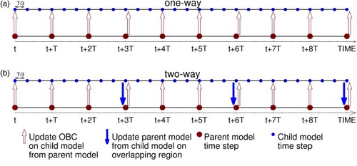
For simplicity but without losing generality, we consider a nested-grid modelling system in which a fine-resolution CM is embedded inside a coarse-resolution PM, with a grid refinement in only the horizontal direction (Fig. 1a). We also assume the ratio of the grid spacing between the PM and CM to be an odd number (which is set to three in our study) in order for cell edges and faces of the PM to coincide with edges and faces of the CM. Furthermore, we consider only the grid point for the pressure variable (or temperature or salinity) in the presentation of the methodology. Figure 1b shows the spatial arrangement of the child grid (blue dots) and the parent grid (red dots) and the dynamical boundary between the CM and the PM. The region inside the thick black line in Fig. 1b represents the computational domain of the CM. There are two sets of ghost cells around the CM boundary in each direction (light blue dots in Fig. 1b) for implementation of the open boundary conditions. The nested-grid system also allows temporal refinement, which is illustrated by the integration flow chart shown in Fig. 2. A time refinement factor of three is used in this study, which is the same as the spatial grid refinement.

Fig. 1 (a) Schematic of a fine-resolution child model (CM) nested inside a coarse-resolution parent model (PM) with a horizontal refinement factor of three. (b) Gridpoint arrangements of the PM and CM over the CM domain. (c) The feedback interface zone (areas marked in red) close to open boundaries of the CM in two-way nesting.

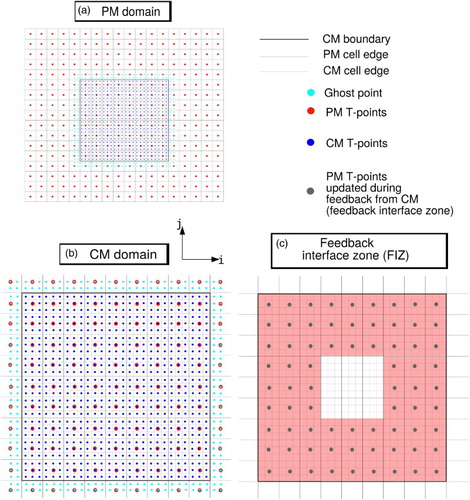
Fig. 2 Time integration in (a) one-way and (b) two-way nesting with the temporal refinement factor of three and update of open boundary conditions (OBC) in the child model every parent model time step (T = Δt_PM)_.

The Adaptive Grid Refinement in Fortran (AGRIF) software is used for nesting in this study, which is a package for adaptive mesh refinement within a finite difference model written in Fortran 90 (Debreu & Blayo, 2002). In this study we use the horizontal and temporal refinement of AGRIF for fixed grids. The AGRIF software allows the interaction between the CM and PM to be either one-way or two-way, depending on the direction of information transferred between the PM and CM. A general description of these approaches is discussed in the following.

a One-Way Nesting

For a one-way nesting configuration, the open boundary conditions for the CM are specified using prognostic variables (temperature, salinity, and currents) of the PM which are interpolated onto the CM grid between two consecutive time steps in the PM. A sponge layer of enhanced viscosity near the CM boundary is applied to smooth inconsistencies between the PM and CM. The following steps elucidate the integration sequence for a time refinement factor of three (Fig. 2a). Assuming all model variables at time t are known, the PM is integrated from time t to t + Δt_PM. The PM variables are linearly interpolated in time at intervals separated by Δt_PM/3 onto the corresponding CM time steps. Because interpolated PM variables at each CM time step are still on the PM grid, they are spatially interpolated onto the CM grid points over the feedback interface zone (FIZ). In this study, the pressure, temperature, and salinity variables are linearly interpolated from the PM grid onto the CM grid and the velocity variables use a nearest-neighbour interpolation in space which satisfies the conservation of model variables during the interpolation step. Once the open boundary conditions for the CM have been obtained, the CM is integrated Δt_PM ∕Δt_CM times until the CM reaches t + Δt_PM. The PM is then advanced and the above procedure is repeated. It is readily seen that for one-way nesting there is no feedback from the CM to PM and the CM can be run offline. As mentioned above, the disadvantage of the one-way nesting approach is that the PM with a coarse resolution does not benefit from the finer resolution results produced by the CM; therefore, dynamical inconsistencies in results produced by the PM and CM could occur, which will be discussed further in Section 4.

b Two-Way Nesting

The first step in two-way nesting is the specification of open boundary conditions for the CM in the same way as in one-way nesting. The second step is the feedback of CM variables to the PM (Fig. 2b). The feedback from the CM to PM can take place over the entire domain of the CM, or over a FIZ close to open boundaries of the CM (Fig. 1c). The FIZ consists of three and two PM grid points in each direction for tracers and currents, respectively. The feedback over the entire domain can take place at time intervals NΔt_PM during the integration of the PM, where N is an integer equal to or larger than 1. Over the FIZ, however, the feedback occurs every Δt_PM time steps.

The AGRIF software provides three types of spatial interpolations for the feedback from the CM to PM: (i) the direct copy from the child to the parent grid (available when an odd horizontal refinement factor is used); (ii) spatial averaging; and (iii) a full weighting scheme. In this study only spatial averaging is used, which means that for a space refinement factor of three a simple average of nine CM grid cells around each PM grid cell is made. This filters out small-scale features in the CM that could introduce numerical noise in the PM (Debreu & Blayo, 2008); therefore, information passed from the CM to PM has horizontal scales that are well resolved by the PM. This interpolation method, however, does not ensure conservation through the CM and PM interface because the PM results are no longer the same as those used to obtain open boundary conditions for the CM. This weakens the coupling between the CM and PM and could create biases over time. Some alternative methods have been suggested to improve this feature in two-way nesting systems, including a flux correction method at the FIZ suggested by Debreu and Blayo (2008) and an implicit nesting in time and space suggested by Haley and Lermusiaux (2010). The implementation of these methods, however, is beyond the scope of the present study.

c Two-Way Nesting Technique Based on the Semi-Prognostic Method

In the conventional two-way nesting technique already discussed, numerical noise could be generated in the PM because PM variables over the overlapping region are constrained by the CM results, and outside the overlapping region the PM variables are purely prognostic and not constrained directly by the CM results. An alternative to the conventional two-way nesting technique is the use of the semi-prognostic method to transfer information from the CM to the PM as suggested by Sheng et al. (2005). By using the semi-prognostic method, the temperature and salinity fields in the PM are prognostic over the entire domain, and numerical noise in the tracer fields resulting from the nesting will be eliminated. This makes the two-way nesting technique based on the semi-prognostic method very attractive, especially in the study of tracer distributions in the ocean.

In the semi-prognostic method, the hydrostatic equation in the PM is modified based on:(1) where is the pressure in the PM, which is used to calculate the horizontal pressure gradient in the horizontal momentum equations of the PM, the PM density, the CM density interpolated onto the PM grid; g is the acceleration due to gravity, and the angle brackets represent a smoothing operator to choose the spatial scales of the feedback from CM to PM. In Eq. (1), β is a coefficient ranging between 0 and 1, which determines the strength of the feedback from CM to PM. For β = 1, the density of the CM does not affect the PM, and the nesting becomes one-way. For β = 0, the density of the CM is used to calculate the vertical pressure gradient in the PM shown in Eq. (1). This study will examine the application of the semi-prognostic method as an alternative to the conventional two-way nesting technique.

3 Nested-grid shelf circulation modelling system

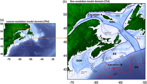
The regional shelf circulation modelling system for the eastern Canadian shelf developed by Urrego-Blanco and Sheng (2014) is used in this study to assess the performance of different nesting techniques. The nested-grid modelling system is based on the coupled ocean–ice NEMO modelling system. The ocean component of the system is based on the primitive equation, second-order of accuracy, z-coordinate Océan PArallélisé, version 9 (OPA9) model. The sea-ice component is based on the two-category, dynamic-thermodynamic Louvain-la-Neuve Ice Model, version 2 (LIM2). The nested-grid modelling system consists of a coarse-resolution PM with a nominal horizontal resolution of 1/4° covering the North Atlantic between 34°N and 55°N and between 33°W and 80°W, as well as a fine-resolution CM with a nominal horizontal resolution of 1/12°, which includes the Gulf of St. Lawrence, the Scotian Shelf, and the Gulf of Maine between 41°N and 52°N and between 55°W and 72°W (Fig. 3). Both the PM and CM use the same 46 z-levels with partial cells in the vertical. The PM uses a time step Δt_PM = 30 min and the CM uses a time step Δt_CM = 10 min. The coupling between the PM and CM is made using AGRIF as described in Section 2. Both the PM and CM use horizontal curvilinear grids and bathymetries extracted from Earth Topography 2 (Smith & Sandwell, 1997). The initial conditions of the modelling system are a state of rest, with initial model temperature and salinity set to the monthly-mean hydrography of Geshelin, Sheng, and Greatbatch (1999). The sea surface salinity is also restored to the climatological monthly-mean surface salinity. The subgrid-scale horizontal mixing of tracers and momentum uses a biharmonic friction with a grid-size dependent Smagorinsky-like mixing (Griffies & Hallberg, 2000), and the subgrid-scale vertical mixing is parameterized using the turbulent closure scheme of Gaspar, Grégoris, and Lefevre (1990). The nested-grid modelling system uses spectral nudging (Thompson, Ohashi, Sheng, Bobanovic, & Ou, 2007) and semi-prognostic methods (Sheng, Greatbatch, & Wright, 2001) to reduce seasonal bias and drift in the modelling system as described by Urrego-Blanco and Sheng (2012). Spectral nudging is applied in both the PM and CM by restoring the annual cycles of temperature and salinity to a 1/6° climatology (Geshelin et al., 1999) regridded onto the CM and PM grids. The spectral nudging uses a relatively weak restoring time scale of 200 days to reduce the model drift in both the PM and CM. It should be noted that spectral nudging and semi-prognostic methods adjust the model dynamics on seasonal or longer time scales and do not affect the characteristics of nesting interactions considered in this study.

Fig. 3 (a) Domain and major bathymetric features of the coarse-resolution parent model of the Northwest Atlantic, with the child model domain marked by dashed lines. (b) Domain and major bathymetric features of the child model for the Gulf of St. Lawrence (GSL), Scotian Shelf (SS), Gulf of Maine (GOM), and Slope Water (SW). Abbreviations used in (b) are Anticosti Gyre (AG), Gaspé Current (GC), Nova Scotia Current (NSC), shelf-break jet (SBJ), Slope Water Jet (SWJ), inflow from the Strait of Belle Isle (ISBI), and inflow of the Labrador Current (ILC).

The nested-grid modelling system is integrated for five years from January 2000 to December 2004 and forced by wind stress and net heat and freshwater fluxes at the sea surface computed from the atmospheric reanalysis fields of Large and Yeager (2004). The reanalysis used here consists of 6-hourly fields of wind speed, specific humidity, and air temperature at 10 m above sea level, 12-hourly fields of short- and longwave radiation, and monthly precipitation. The modelling system is also forced by monthly-mean river runoff based on the global monthly streamflow dataset of Dai, Qian, and Trenberth (2009). The river discharge of each river is specified in terms of precipitation over a specific influence area in the model. The area of influence is determined using a radius of influence proportional to the monthly river discharge. The reader is referred to Urrego-Blanco and Sheng (2014) for details on the methodology used to prescribe river runoff in the model. The open boundary conditions in the PM are taken from the five-day mean ocean reanalysis data of Smith, Haines, Kansow, and Cunningham (2010). More details on the model forcing, lateral open boundary conditions, and model validation can be found in Urrego-Blanco and Sheng (2012) and Urrego-Blanco and Sheng (2014).

To examine the performance of different nesting techniques, model results in the following five numerical experiments are used:

1. Experiment TWN-CR: This is the control run in which the external forcing discussed above and the conventional two-way nesting are used. The feedback from the CM to PM takes place over the entire domain, with the exchange frequency of 3Δt_PM, or 1.5 hours.

2. Experiment OWN: The model setup and forcing in this case are the same as in TWN-CR except that the interaction between the PM and CM is only one-way as discussed in Section 2.a. Model results in this experiment are used to demonstrate the model inconsistencies between the CM and PM when no feedback occurs from CM to PM.

3. Experiment TWN-SP: In this experiment the semi-prognostic method is used as a two-way nesting technique. The model forcing and setup in this case are the same as in the control run except that temperature, salinity, and currents in the CM do not feed back directly onto the PM over the entire CM domain. Instead, the CM density calculated from the CM temperature and salinity is used to update the hydrostatic equation of the PM based on Eq. (1) with β = 0. In this experiment there is no spatial smoothing applied to the difference between the CM and the PM densities in Eq. (1). However, the CM density is spatially smoothed by interpolating the nine neighbouring CM values from the CM grid onto the PM grid. This experiment is used to demonstrate the advantage of the semi-prognostic method used as a two-way nesting technique in reducing numerical noise resulting from the feedback from CM to PM.

4. Experiment TWN-20D: This experiment is same as the control run except that the exchange frequency between the PM and CM is 960Δt_PM, or 20 days. The model results in this experiment are used to examine how frequent the two-way coupling between the PM and CM should be in order to generate dynamically consistent subtidal circulation.

5. Experiment TWN-BND: In this experiment two-way interaction between the PM and CM occurs only over their dynamical interface (FIZ zone). The exchange frequency is Δt_PM, or 0.5 hours. Results in this case are used to examine the limitation of the two-way coupling occurring only over the FIZ.

4 Results

In this section, the model results from the control run (TWN-CR) are first presented to demonstrate the performance of the nested-grid model with the default setup and model forcing. Comparisons of model results in different numerical experiments will then be used to assess the performance of different nesting techniques.

a Model Results in the Control Run

Figures 4 and 5 present the five-day mean fields of temperature and currents on 7 July 2004 produced by the PM and CM at 9 and 100 m, respectively. The near-surface circulation produced by the PM (Fig. 4a) features the northeastward flow associated with the Gulf Stream and temperatures above 20°C in the deep waters of the Slope Water region, the north and northeastward flow of the North Atlantic Current, and the equatorward flowing Labrador Current along the shelf break of the Labrador Shelf. All these large-scale circulation features produced by the PM are in good agreement with the general knowledge of circulation in this region. On 7 July 2004, near-surface temperatures of about 8°C are found over the Labrador Shelf, in the Gulf of St. Lawrence, and over the eastern Scotian Shelf, and slightly warmer temperatures are found in the Gulf of Maine and over the western Scotian Shelf (∼12°C). In comparison with the PM results, the CM reproduces more realistically the southeastward flow from the lower St. Lawrence Estuary to Cabot Strait and the southwestward flowing Nova Scotia Current along the inner Scotian Shelf as a result of the finer horizontal resolution used in the CM (Fig. 4b). A comparison of Figs 4a and 4b indicates that large-scale circulation features in the PM and the CM are very similar, except that the model results in the CM have more small-scale features.

Fig. 4 Five-day mean fields of temperature and currents at 9 m on 7 July 2004 produced by (a) the PM and (b) the CM in TWN-CR. Velocity vectors are plotted at every third model grid point.

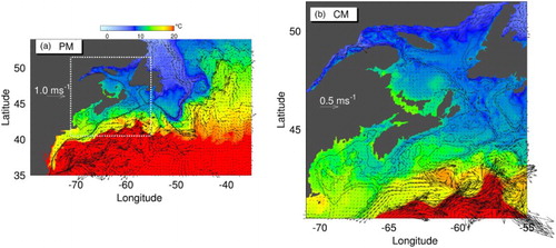
Fig. 5 Five-day mean fields of temperature and currents at 100 m on 7 July 2004 produced by (a) the PM and (b) the CM in TWN-CR. Velocity vectors are plotted at every third model grid point.

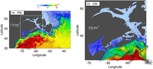
The sub-surface circulation (100 m) over the eastern Canadian shelf produced by the nested-grid modelling system also features the Labrador Current, the Gulf Stream, and the North Atlantic Current (Fig. 5a). In deep waters, the sub-surface currents are weaker than the near-surface currents (Figs 4b and 5b). Over the shelf region, the near-surface and sub-surface temperatures decrease significantly, with warmer waters lying on top of cold waters, which is consistent with the observed vertical thermal structure of the waters in summer months over the region (Banks, 1966; Drinkwater & Gilbert, 2004).

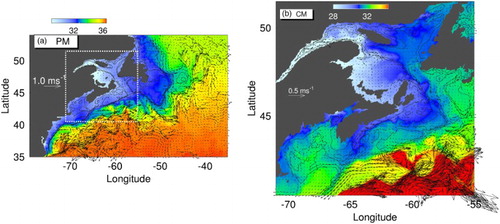
The near-surface salinity distribution on 7 July 2004 produced by the PM is significantly fresher over the eastern Canadian shelf and saltier over deep waters of the Northwest Atlantic Ocean (Fig. 6a). This is mainly due to the combined effect of equatorward propagation of low-salinity waters from high latitudes and freshwater discharge from rivers over coastal and shelf regions. A comparison of Figs 6a and 6b indicates that the estuarine circulation associated with the river discharge into the western Gulf of St. Lawrence, over the inner Scotian Shelf, and into the coastal waters of the Gulf of Maine is better simulated by the CM than by the PM. For instance, instabilities in the Gaspé current and the freshwater plume of the St. John River are simulated by the CM but not by the PM (Fig. 6).

Fig. 6 Five-day mean fields of salinity and currents at 9 m on 7 July 2004 produced by (a) the PM and (b) the CM in TWN-CR. Velocity vectors are plotted at every third model grid point.

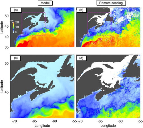
To demonstrate the performance of the nested-grid system, the five-day mean near-surface (3 m) temperatures on 7 February 2003 produced by the PM and CM in TWN-CR are compared with the sea surface temperature (SST) estimated from the remotely sensed data (Fig. 7) provided by the Maurice Lamontagne Institute. It should be noted that the remotely sensed SST data are not available everywhere, particularly during winter in the Gulf of St. Lawrence and over the Newfoundland and Labrador Shelves because of cloud cover and/or the presence of sea ice (Figs 7b and 7d). Comparison of Figs 7a and 7b indicates that the large-scale SST features derived from the remotely sensed data are reproduced reasonably well by the PM. The PM also generates relatively warm surface temperatures in the deep waters of the Northwest Atlantic and relatively colder surface waters over the continental shelf region on that day. The observed position of the frontal region between the warm and cold waters is reasonably reproduced by the PM. The PM, however, slightly overestimates the near-surface temperature in the deep waters (Figs 7a and 7b). Comparison of Figs 7c and 7d also demonstrates that the near-surface temperatures in the CM agree reasonably well with the observed SSTs, particularly over the western Scotian Shelf and in the Gulf of Maine. It should be noted that the nested-grid modelling system does not assimilate observations, except for a weak nudging of the annual cycles of climatological temperature and salinity using the spectral nudging method as mentioned in Section 3. It is not surprising, therefore, that small-scale features of circulation, such as eddies and meanders, produced by the CM, particularly over the Slope Water region, do not agree as well with the observations.

Fig. 7 Comparison of simulated (a) and (c) and observed (b) and (d) 5-day mean sea surface temperatures over the PM domain (upper panels) and the CM domain (lower panels) in the TWN-CR experiment on 7 February 2003. White areas in (b) and (d) mean that the remotely sensed SST data over these areas were missing because of cloud cover or the presence of sea ice.

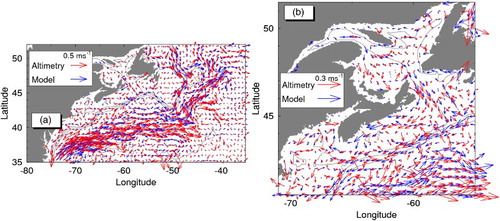
Figure 8a presents a comparison the time-mean surface geostrophic currents estimated from the time-mean sea surface elevation in the PM for 2001–2004 with the observed currents derived from altimetry (Higginson, Thompson, Huang, Véronneau, & Wright, 2011). The general observed circulation features associated with the Gulf Stream, the North Atlantic Current, and the inshore and offshore branches of the Labrador Current are reproduced reasonably well by the PM. Figs 8b presents time-mean surface geostrophic currents estimated from altimetry and calculated from the CM results. The time-mean circulation produced by the CM is characterized by a westward flow along the northern Québec shore, a cyclonic circulation over the northwestern Gulf of St. Lawrence to the west of Anticosti Island, and a recirculation of the flow southeast of Anticosti Island. The CM also generates an inflow (outflow) over eastern (western) Cabot Strait, a southwestward flow along the Scotian Shelf, and a cyclonic circulation in the Gulf of Maine. Qualitatively, these time-mean circulation features produced by the CM are in good agreement with the surface geostrophic currents derived from altimetry. The reader is referred to Urrego-Blanco and Sheng (2012, 2014) for further discussion on the performance of the nested-grid system.

Fig. 8 Comparison of time-mean geostrophic currents from 2001 to 2004 calculated from the simulated (blue) and altimetry-derived (red) time-mean sea surface elevations (altimetry data from Higginson et al., 2011). The simulated results are calculated by (a) the PM over the Northwest Atlantic Ocean and (b) the CM over the eastern Canadian shelf from the Gulf of St. Lawrence to the Gulf of Maine. Velocity vectors are plotted at (a) every third PM grid point and (b) every sixth CM grid point.

b Performance of One-Way and Two-Way Nesting Techniques

To further demonstrate the advantage of conventional two-way nesting, we examine the dynamical consistency between the PM and CM results. The five-day mean CM and PM results of salinity and currents in TWN-CR and OWN on 17 July 2004 are presented in Fig. 9. The near-surface salinity fields produced by the CM and PM are very similar in TWN-CR (Figs 9a and 9b), with relatively high salinity over the Slope Water region and low salinity over the western Gulf of St. Lawrence and coastal waters of the Scotian Shelf. The two-way nesting approach ensures that the circulation produced by the PM and CM is dynamically consistent. For instance, an anticyclonic eddy centred at about 62°W and 42°N occurs in both the CM and the PM on 17 July. A salinity front in the central Gulf of St. Lawrence and the freshwater plume extending down to the western Scotian Shelf are also reproduced well by the CM and PM in the case of two-way nesting.

Fig. 9 Comparison of five-day mean near-surface (9 m) salinity and currents simulated by the CM (left panels) and PM (right panels) over the CM domain on 17 July 2004 for (a) and (b) TWN-CR and (c) and (d) OWN. Velocity vectors are plotted at every sixth child model grid point.

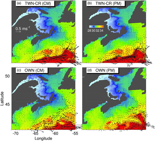
Figures 9c and 9d present five-day mean near-surface circulation and salinity fields produced by the PM and CM for OWN. The use of the one-way nesting technique leads to significant differences in the circulation produced by the PM and CM. Over the lower St. Lawrence Estuary, for example, the near-surface salinity is much fresher in the PM than in the CM. The influence of the freshwater plume over coastal waters of the Scotian Shelf is more intense in the CM than in the PM. The shelf-break jet is significantly stronger in the CM than in the PM. There are also significant differences over the Slope Water region where mesoscale features appear over different areas in the CM and PM with OWN.

We next examine the effect of data exchange frequencies in two-way nesting on the dynamical consistency of model results produced by the CM and PM. Figures 10a and 10b present the five-day mean near-surface salinity and currents on 17 July produced by the CM and PM, using the exchange frequency of 20 days in TWN-20D. The large-scale patterns in TWN-20D are characterized by relatively fresher waters over the western Gulf of St. Lawrence and relatively saltier waters over the Slope Water region in the CM and PM. This less frequent data exchange between the CM and PM still produces a large-scale subtidal circulation that is reasonably consistent between the different model components in TWN-20D. For smaller-scale subtidal circulation features, however, the PM and CM results differ over several regions such as the lower St. Lawrence Estuary, the coastal waters of the Scotian Shelf, and estuarine waters in the northern Gulf of St. Lawrence, and the Gulf of Maine. It should be noted that the main focus here is on the effect of different nesting techniques on the subtidal circulation. For circulation with high-frequency variability, an exchange frequency of 20 days would not ensure dynamical consistency between the PM and CM.

Fig. 10 Comparison of five-day mean near-surface (9 m) salinity and currents simulated by the CM (left panels) and PM (right panels) over the CM domain on 17 July 2004 for (a) and (b) TWN-20D and (c) and (d) TWN-BND. Velocity vectors are plotted at every sixth child model grid point.

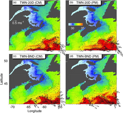
The results produced by the CM and PM are presented in Figs 10c and 10d, with the feedback taking place only over the FIZ (TWN-BND). In this case, there are significant differences in the near-surface salinity fields produced by the PM and CM. In comparison with the CM results, the propagation of the low-salinity estuarine plume, emanating from the western Gulf of St. Lawrence through Cabot Strait and affecting the inner Scotian Shelf, is not reproduced well by the PM (Figs 10c and 10d). The near-surface salinity over the western Gulf of St. Lawrence, central Scotian Shelf, and Gulf of Maine in TWN-BND is higher in the PM than in the CM. Finally, the circulation over the Slope Water region, simulated by the PM in this case, does not agree well with the flow field produced by the CM. Therefore, the interaction between the CM and PM over the FIZ is not sufficient to generate dynamically consistent circulation and hydrography between the CM and PM.

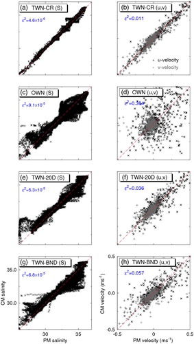
To quantify the consistency between PM and CM results, we introduce ε² defined as:where is a PM variable and is a CM variable; N is the number of PM grid points that lie within the CM domain. The overbar indicates the mean of the PM and CM variables. The agreement between PM and CM is perfect if ε² = 0, and the consistency between PM and CM decreases as ε² increases. Figure 11 presents scatterplots of the CM and PM results and the corresponding ε² values in four different cases (TWN-CR, OWN, TWN-20D, and TWN-BND). The largest values of ε² in the four cases shown in Fig. 11 occur in OWN, indicating significant inconsistency between PM and CM results if nesting is one-way. In this case ε² has values of about 0.104 for salinity and 1.24 for currents. The dynamical consistency between the PM and CM results improves significantly in TWN-CR, with ε² values of 5 × 10^–3 for salinity and 0.041 for currents. In comparison with results in OWN, model results in TWN-20D and TWN-BND also significantly improve the consistency between PM and CM with smaller ε² values than in OWN.

Fig. 11 Scatterplots of salinity (left panels) and currents (right panels) produced by the PM and CM over the CM domain on 17 July 2004 for (a) and (b) TWN-CR; (c) and (d) OWN; (e) and (f) TWN-20D; and (g) and (h) TWN-BND.

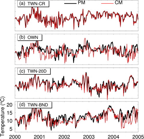
Figures 12 and 13 present time series of model salinity and temperature at locations A and B produced by the PM and CM in four numerical experiments (TWN-CR, OWN, TWN-20D, and TWN-BND). These two locations are in the lower St. Lawrence Estuary and in the Slope Water region, respectively, as marked in Fig. 3. In TWN-CR, the sub-surface salinities and temperatures (Figs 12a and 13a) in the CM and PM agree well at these two locations, as expected. By comparison, the sub-surface salinity at location A produced by the CM in OWN compares well with the results in TWN-CR, but the PM results in OWN differ significantly from the CM results in TWN-CR (Fig. 12b). This indicates that the PM performs less well because of the lack of feedback from the CM to PM. The sub-surface salinity produced by the PM and CM agrees better in TWN-20D (Fig. 12c) than in OWN (Fig. 12b). There are large differences between the PM and CM model results in TWN-20D because of the less frequent information exchange between the PM and CM. It should be noted that the model results have more high-frequency variability in TWN-20D than TWN-CR. In TWN-BND the CM results are similar to the CM results in TWN-CR, but the PM performs less well and drifts from the CM results if only information at the FIZ is exchanged (Fig. 12d). At location B, situated over the Slope Water region (Fig. 3), the time series of sub-surface temperature display significant high-frequency variability (Fig. 13). The sub-surface time series of temperature produced by the PM differs significantly from the CM results in the cases of OWN and TWN-BND (Figs 13b and 13d), with the largest differences occurring in OWN. The CM results in OWN, TWN-20D, and TWN-BND differ from the CM results in TWN-CR, indicating that more frequent information exchange is needed over the entire overlapping area between the CM and PM.

Fig. 12 Time series of the five-day mean sub-surface (32 m) salinity at location A (see Fig. 3) over the northwestern Gulf of St. Lawrence produced by the PM (black) and CM (red) for (a) TWN-CR, (b) OWN, (c) TWN-20D, and (d) TWN-BND.

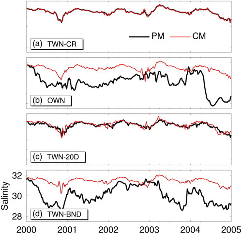
Fig. 13 Time series of the five-day mean sub-surface (100 m) temperature at location B (see Fig. 3) over the Slope Water region off the Scotian Shelf produced by the PM (black) and CM (red) for (a) TWN-CR, (b) OWN, (c) TWN-20D, and (d) TWN-BND.

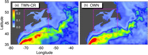
To further demonstrate the advantage of feedback from the CM to the PM, we compare the standard deviation of sea surface elevations produced by the PM in the cases of TWN-CR and OWN. Figure 14 presents the standard deviations of sea surface elevations from 2001 to 2004 produced by the PM in the two cases. In comparison with the PM results in OWN (Fig. 14a), the PM results in TWN-CR (Fig. 14b) have more variability in sea surface elevation indicating an improvement in the circulation in the PM when two-way nesting is applied. The higher variability produced by the PM in TWN-CR occurs not only over the overlapping region between the CM and PM but also over regions outside the overlapping region, including areas directly affected by the Gulf Stream and the North Atlantic Current.

Fig. 14 Time-mean standard deviations of sea surface elevations from 2001 to 2004 produced by the PM for (a) OWN and (b) TWN-CR. The region marked by dashed lines is the CM domain.

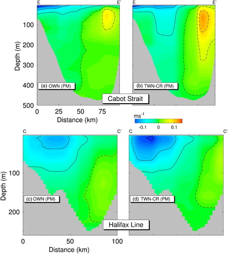
We next examine the improvement in the regional circulation over coastal waters of the eastern Canadian shelf in the PM achieved by using two-way nesting. Figures 15a and 15c show the 2001–2004 time-mean currents normal to the transects shown in Fig. 3 at Cabot Strait and the Scotian Shelf (Halifax Line) produced by the PM in OWN. The PM results in TWN-CR feature generally stronger coastal currents than in OWN (Figs 15b and 15d). In particular, the inflow into the Gulf of St. Lawrence at the eastern side of Cabot Strait is stronger and the outflow from the Gulf of St. Lawrence at the western side of the Strait extends deeper throughout the water column in TWN-CR (Fig. 15b) than OWN (Fig. 15a. In TWN-CR, the estimated time-mean outflow at Cabot Strait in the PM is about 0.67 Sv (1 Sv = 10⁶ m³ s^–1). This value is close to estimates from other modelling studies, which suggests that the time-mean outflow at the western Cabot Strait is about 1.02 Sv (Han, Loder, & Smith, 1999). By comparison, in OWN the estimated transport in the PM is only 0.38 Sv. The Nova Scotia Current in the PM is also stronger in TWN-CR than in OWN. The maximum speeds are about 0.18 m s⁻¹ in TWN-CR and about 0.12 m s⁻¹ in OWN (Figs 15c and 15d). The time-mean volume transport of the Nova Scotia Current in TWN-CR is about 0.61 Sv, which is in good agreement with the observational estimate of 0.75 Sv of Loder, Hannah, Petrie, and Gonzales (2003). By comparison, the time-mean transport of the Nova Scotia Current in OWN is only 0.53 Sv.

Fig. 15 Time-mean normal velocities at Cabot Strait and the Halifax Line from 2001 to 2004 produced by the PM for (a) and (c) OWN and (b) and (d) TWN-CR. Contour lines are spaced at 0.05 m s⁻¹.

c Performance of the Two-Way Nesting Technique Based on the Semi-Prognostic Method

The conventional two-way nesting technique could lead to generation of numerical noise in the PM because of the shock produced during the feedback from the CM to PM. Figures 16a and 16b present a 30-day time series of simulated sub-surface salinity at location B (see Fig. 3) in experiments TWN-CR and TWN-20D, respectively. The shocks introduced during the feedback in TWN-20D are obvious on days 140 and 160 in 2000 but are less obvious in TWN-CR. Figure 17 shows the same time series over a two-day period (shaded interval in Fig. 16) in 2000. Although numerical noise also occurs in TWN-CR, the largest amplitudes of numerical noise occur in TWN-20D. However, the effect of the numerical shock persists throughout the entire record in TWN-CR (Fig. 17a) and decays faster in TWN-20D (Fig. 17b).

Fig. 16 Time series of instantaneous sub-surface (100 m) salinity at location B (see Fig. 3) over the Slope Water region off the Scotian Shelf produced by the PM (black) and the CM (red) between 1 June 2000 and 30 June 2000 for (a) TWN-CR, (b) TWN-20D, and (c) TWN-SP.

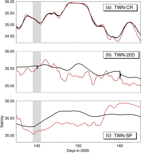
Fig. 17 Time series of instantaneous sub-surface (100 m) salinity at location B (see Fig. 3) over the Slope Water region off the Scotian Shelf produced by the PM (black) and the CM (red) between 19 May 2000 and 20 May 2000 (shaded period in Fig. 16) for (a) TWN-CR, (b) TWN-20D, and (c) TWN-SP.

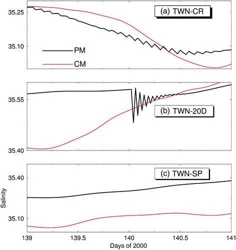
We next examine the performance of the two-way nesting technique based on the semi-prognostic method (TWN-SP). In this case, the CM temperature and salinity are used to update the hydrostatic pressure equation in the PM, which in turn affects the 3D circulation in the PM.

Figures 16c and 17c demonstrate that the PM results in TWN-SP do not have numerical noise resulting from the feedback of the CM density to the PM. Because temperature and salinity in the PM are not directly affected by the CM results during the feedback step, two-way nesting based on the semi-prognostic method has a major advantage over conventional two-way nesting in simulating tracers by the PM. It should be noted that the TWN-SP method does not guarantee that the temperature and salinity will be the same in the PM and CM over the overlapping region because the hydrography in the PM over the overlapping region is not constrained directly by the CM results in this method.

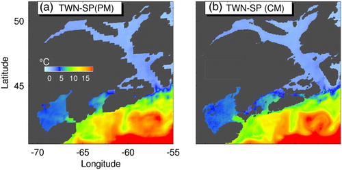
We next examine the dynamical consistency between CM and PM results in TWN-SP. Figures 18a and 18b show the five-day mean fields of sub-surface (32 m) temperatures on 29 December 2001 produced by the PM and CM, respectively, in TWN-SP. The PM and CM results are reasonably consistent in this experiment. The large-scale temperature fields in both the PM and CM in TWN-SP feature cold water less than 2.5°C over the Gulf of St. Lawrence and the eastern Scotian Shelf. Over the Gulf of Maine and the southwestern Scotian Shelf, water temperatures are slightly above approximately 5°C, and over the deepest part of the Slope Water region the water temperature ranges from 13° to 17°C. The temperature fields in Figs 18a and 18b show some differences in small-scale structures produced by the PM and CM, which is mainly a result of the finer resolution of the CM. For deeper waters, greater than 100 m, Figs 19a and 19b also show good agreement in the large-scale temperature fields in the CM and PM, with some minor differences in mesoscale features.

Fig. 18 Comparison of five-day mean sub-surface temperature (32 m) on 29 December 2001 over the CM domain produced by (a) the PM and (b) the CM in TWN-SP.

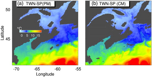
Fig. 19 Comparison of five-day mean temperature at 100 m on 26 August 2004 over the CM domain produced by (a) the PM and (b) the CM in experiment TWN-SP.

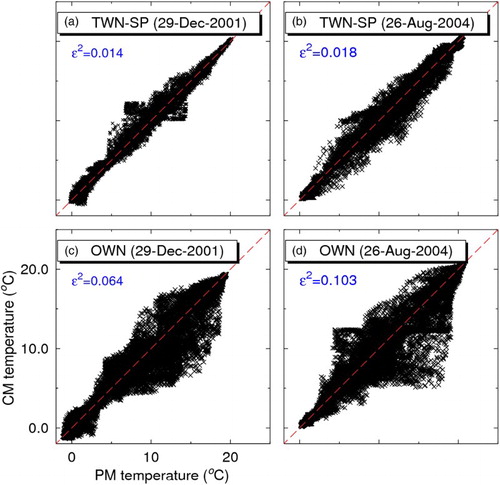
To further quantify the consistency of CM and PM results in TWN-SP in Figs 18 and 19, we present scatterplots of CM and PM temperature and their ε² values in Figs 20a and 20b. The scatterplots indicate that the PM and CM results are consistent in TWN-SP (Figs 20a and 20b) with some degree of scatter about the line of perfect agreement. Figures 20c and 20d show that the spread of CM and PM results about the line of perfect agreement is still significantly smaller in TWN-SP than in OWN. The ε² values in Fig. 20 are 0.014 and 0.018 for TWN-SP, which are significantly smaller than the ε² values of 0.064 and 0.103 for OWN, with ε² values in TWN-SP being about five times less than in OWN. The ε² values are somewhat higher than the values of about 0.009 in TWN-CR (not shown), indicating that the CM and PM results are slightly more consistent in the latter experiment. This is also consistent with stronger coupling in TWN-CR than in TWN-SP. Therefore, the TWN-SP has an advantage in producing consistent CM and PM results and eliminating numerical noise resulting from the interaction of model components.

Fig. 20 Scatterplots of temperature simulated by the PM and the CM on 29 December 2001 (left panels) and 26 August 2004 (right panels) for (a) and (b) TWN-SP and (c) and (d) OWN.

5 Summary and conclusions

Our study assessed the performance of three different nesting techniques: conventional two-way nesting; one-way nesting; and two-way nesting based on the semi-prognostic method (TWN-SP). The assessment was made in terms of four aspects: (i) dynamical consistency between the PM and CM results, (ii) improvement of the large-scale circulation in the PM, (iii) improvement of the regional circulation in the CM, and (iv) the reduction of numerical noise in the PM generated by feedback of model variables from the CM to the PM.

The nested-grid circulation modelling system for the eastern Canadian shelf was used in this study. The main circulation features over the eastern Canadian shelf were reproduced reasonably well by the modelling system using the conventional two-way nesting approach (TWN-CR). It was demonstrated that two-way nesting techniques perform better than the one-way nesting technique. In particular, two-way nesting ensures dynamical consistency between CM and PM results when feedback from the CM to the PM occurs frequently. By comparison, the PM results for the OWN experiment drift from the CM results. It was also demonstrated that two-way coupling between the CM and PM taking place only over the FIZ does not guarantee dynamical consistency between PM and CM results. Therefore, nested-grid ocean models should implement two-way coupling between the CM and PM over the entire CM domain. The use of a less frequent exchange between the CM and PM in the two-way configuration (TWN-20D) led to relatively good agreement between CM and PM results for subtidal circulation. However, more frequent exchange between the PM and CM is needed for simulating high-frequency variability of the model fields.

The variability of the sea surface elevation produced by the PM in the case of TWN-CR was larger than for OWN, indicating that two-way nesting improves the large-scale circulation in nested-grid ocean models. The enhanced sea surface elevation variability in two-way nesting not only occurs over the overlapping region between the CM and PM but also over regions outside the overlapping region, including the Slope Water region and the northwest corner of the North Atlantic Current. Another advantage of using two-way nesting instead of one-way nesting is the improvement in regional circulation features in the PM. In particular, coastal currents are more realistically reproduced by the PM in TWN-CR than in the OWN experiment. In two-way nesting the higher horizontal resolution of the CM and the feedback of model results to the PM lead to generally stronger and more realistic coastal currents than in OWN.

It was found, however, that numerical noise can be generated by conventional two-way nesting. To eliminate this type of noise we implemented a two-way nesting technique based on the semi-prognostic method (TWN-SP) in which the temperature and salinity in the CM are used to add a correction term to the horizontal pressure gradients in the momentum equation for the PM. The main advantages of the TWN-SP are (i) the elimination of numerical noise during the feedback of the CM to PM as a result of weaker coupling between model grids and (ii) the dynamical consistency between PM and CM results. The TWN-SP is, therefore, a very attractive method to use in modelling studies of tracers in the ocean.

As a final remark, our results suggest that embedded modelling systems should use two-way nesting techniques with feedback from the CM to the PM over the entire overlapping area (TWN-CR, TWN-20D, and TWN-SP) to ensure dynamical consistency between the PM and CM. Our results also suggest that the TWN-SP is the best method for eliminating noise in the PM during feedback from the CM to PM and having dynamical consistency with other nesting techniques (Table 1). Furthermore, two-way nesting techniques with low feedback frequencies (TWN-20D) should be avoided if the interest is high-frequency variability, unless numerical noise can be effectively reduced during update from CM to PM.

Table 1. Summary of numerical experiments conducted in this study.

Experiment	Feedback over entire CM domain	Noise generated on PM	Consistency between CM and PM
TWN-CR	Yes	Yes	Yes
OWN	No	No	No
TWN-20D	Yes	Yes	Yes (only at low frequencies)
TWN-BND	No	No	No
TWN-SP	Yes	No	Yes

Future work includes the improvement of conservation properties between model grids, which could help reduce noise and improve dynamical consistency in the modelling system. Other factors to be further examined include the sensitivity of the performance assessment to the location of CM boundaries, particularly the choice of the southern boundary over a region less affected by the intense mesoscale dynamics associated with the meandering of the Gulf Stream.

Acknowledgements

We wish to thank the anonymous reviewers for very constructive comments and suggestions. We also wish to thank Laurent Debreu for his helpful insights into the AGRIF algorithm and Pierre Larouche for providing remotely sensed data. This study utilized ACEnet computational resources.

Disclosure statement

No potential conflict of interest was reported by the authors.

Additional information

Funding

This study was funded by the Ocean Tracking Network Canada (OTN), the Marine Environmental Observation Prediction and Response Network (MEOPAR), the Natural Sciences and Engineering Council of Canada (NSERC), and the Lloyd's Register Foundation (LRF); LRF helps to protect life and property by supporting engineering-related education, public engagement, and the application of research.

References

- Banks, R. E. (1966). The cold intermediate layer of the Gulf of St. Lawrence. Journal of Geophysical Research, 71, 1603–1610. doi: 10.1029/JZ071i006p01603
- Dai, A., Qian, T., & Trenberth, K. E. (2009). Changes in continental freshwater discharge from 1948 to 2004. Journal of Climate, 22, 2773–2791. doi: 10.1175/2008JCLI2592.1
- Danilov, S., Wang, Q., Losch, M., Sidorrenko, D., & Schröter, J. (2008). Modeling ocean circulation on unstructured meshes: Comparison of two horizontal discretizations. Ocean Dynamics, 58, 365–374. doi:10.1007/s10236-008-0138-5
- Debreu, L., & Blayo, E. (2002). AGRIF: Adaptive grid refinement in Fortran. Tech. Report 0262. Le Chesnay, France: INRIA.
- Debreu, L., & Blayo, L. (2008). Two-way embedding algorithms: A review. Ocean Dynamics, 58, 415–428. doi: 10.1007/s10236-008-0150-9
- Drinkwater, K. F., & Gilbert, D. (2004). Hydrographic variability in the waters of the Gulf of St. Lawrence, the Scotian Shelf and the Eastern Gulf of Maine (NAFO Subarea 4) during 1991–2000. Journal of Northwest Atlantic Fishery Science, 34, 83–99.
- Eden, C., Greatbatch, R. J., & Böning, C. W. (2004). Adiabatically correcting an eddy-permitting model of the North Atlantic using large-scale hydrographic data: Applications to the Gulf Stream and the North Atlantic Current. Journal of Physical Oceanography, 34, 701–719. doi: 10.1175/1520-0485(2004)034<0701:ACAEMU>2.0.CO;2
- Gaspar, P., Grégoris, P., & Lefevre, J. M. (1990). A simple eddy kinetic energy model for simulations of the oceanic vertical mixing tests at Station Papa and long-term upper ocean study site. Journal of Geophysical Research, 96, 16179–16193. doi: 10.1029/JC095iC09p16179
- Geshelin, Y., Sheng, J., & Greatbatch, R. J. (1999). Monthly-mean climatologies of temperature and salinity in the western North Atlantic. Can. Data Rep. Hydrogr. Ocean Sci. No. 153, Dartmouth, Nova Scotia: Fisheries and Oceans Canada.
- Greatbatch, R. J., Sheng, J., Eden, C., Tang, L., Zhai, X., & Zhao, J. (2004). The semi-prognostic method. Continental Shelf Research, 24(18), 2149–2165. doi: 10.1016/j.csr.2004.07.009
- Griffies, M. S., & Hallberg, R. (2000). Biharmonic friction with a Smagorinsky-like viscosity for use in large-scale eddy-permitting ocean models. Monthly Weather Review, 128, 2935–2946. doi: 10.1175/1520-0493(2000)128<2935:BFWASL>2.0.CO;2
- Haley Jr., P. J., & Lermusiaux, P. F. J. (2010). Multiscale two-way embedding schemes for free surface primitive equations in the “Multidisciplinary Simulation, Estimation and Assimilation System”. Ocean Dynamics, 60, 1497–1537. doi: 10.1007/s10236-010-0349-4
- Han, H., Loder, J. W., & Smith, P. C. (1999). Seasonal mean hydrography and circulation in the Gulf of St. Lawrence and on the eastern Scotian and Newfoundland Shelves. Journal of Physical Oceanography, 29, 1279–1301. doi: 10.1175/1520-0485(1999)029<1279:SMHACI>2.0.CO;2
- Herrnstein, A., Wickett, M., & Rodriguez, O. (2005). Structured adaptive mesh refinement using leapfrog time integration on a staggered grid for ocean models. Ocean Modelling, 9(3), 283–304. doi: 10.1016/j.ocemod.2004.07.002
- Higginson, S., Thompson, K. R., Huang, M., Véronneau, M., & Wright, D. (2011). The mean surface circulation of the North Atlantic subpolar gyre: A comparison of estimates derived from new gravity and oceanographic measurements. Journal of Geophysical Research, 116. C08016, doi:10.1029/2010JC006877
- Kurihara, Y., Tripoli, G. J., & Bender, M. A. (1979). Design of a movable nested-mesh primitive equation model. Monthly Weather Review, 107, 239–249. doi: 10.1175/1520-0493(1979)107<0239:DOAMNM>2.0.CO;2
- Large, W., & Yeager, S. (2004). Diurnal to decadal global forcing for ocean and sea-ice models: The data sets and flux climatologies. Tech. Report TN-460 + STR, NCAR. Boulder, Colorado: National Center for Atmospheric Research (NCAR).
- Loder, J. W., Hannah, C. G., Petrie, B. D., & Gonzales, E. A. (2003). Hydrographic and transport variability on the Halifax section. Journal of Geophysical Research, 108(C11), 8003. doi: 10.1029/2001JC001267
- Oey, L. Y., & Chen, P. (1992). A nested-grid ocean model: With application to the simulation of meanders and eddies in the Norwegian Coastal Current. Journal of Geophysical Research, 97, 20063–20086. doi: 10.1029/92JC01991
- Sheng, J., Greatbatch, R. J., & Wright, D. G. (2001). Improving the utility of ocean circulation models through adjustment of the momentum balance. Journal of Geophysical Research, 106, 16711–16728. doi: 10.1029/2000JC000680
- Sheng, J., Greatbatch, R. J., Zhai, X., & Tang, L. (2005). A new two-way nesting technique for ocean modelling based on the smoothed semi-prognostic method. Ocean Dynamics, 55, 162–177. doi: 10.1007/s10236-005-0005-6
- Smith, G. C., Haines, K., Kansow, T., & Cunningham, S. (2010). Impact of hydrographic data assimilation on the modelled Atlantic meridional overturning circulation. Ocean Science, 6, 761–774. doi: 10.5194/os-6-761-2010
- Smith, H. F., & Sandwell, D. T. (1997). Global sea floor topography from satellite altimetry and ship depth soundings. Science., 277, 977–1012. doi: 10.1126/science.277.5328.977
- Thompson, K. R., Ohashi, K., Sheng, J., Bobanovic, J., & Ou, J. (2007). Suppressing bias and drift of coastal circulation models through the assimilation of seasonal climatologies of temperature and salinity. Continental Shelf Research, 27, 1303–1316. doi: 10.1016/j.csr.2006.10.011
- Urrego-Blanco, J., & Sheng, J. (2012). Interannual variability of the circulation over the eastern Canadian Shelf. Atmosphere-Ocean., 50, 277–300. doi: 10.1080/07055900.2012.680430
- Urrego-Blanco, J., & Sheng, J. (2014). Study on subtidal circulation and variability in the Gulf of St. Lawrence, Scotian Shelf and Gulf of Maine using a nested-grid shelf circulation model. Ocean Dynamics, 64, 385–412. doi: 10.1007/s10236-013-0688-z