Preserving Continuity of Long-Term Daily Maximum and Minimum Temperature Observations with Automation of Reference Climate Stations using Overlapping Data and Meteorological Conditions

ABSTRACT

The seasonal-by-wind bias method for aligning time series of daily maximum and minimum temperatures from past conventional staffed and new automated sites using closely collocated, overlapping observations is presented for twenty-two modernized Reference Climate Stations in Canada. The method consists of adjusting for incompatible observing times and deriving biases from the daily “manual-minus-automated” temperature differences classified into seasons and wind-speed conditions. Most of the biases vary with the season, and many show limited wind dependency. Four sets of adjusted time series are prepared based on two-year and five-year overlapping data and on seasonal bias with or without wind conditions; the adjusted data are compared with the original observations. Based on the mean of the absolute differences and examination of box plots, the results show that, for this particular set of stations, the two-year versus five-year and seasonal versus seasonal-by-wind bias adjusted time series are overall similar. The largest contribution to the improvements in the adjusted observations came from matching the times of observation. Additionally, daily temperatures are adjusted using statistical methods applied with neighbouring station data but no overlapping observations at collocated stations; it is concluded that these do not necessarily resolve the bias between staffed and automated sites.

RÉsumé

[Traduit par la rédaction] Nous présentons, pour vingt-deux stations climatologiques de référence canadiennes modernisées, un calcul de biais tenant compte des saisons et des vents, et servant à aligner des séries temporelles de températures journalières maximales et minimales, issues d'anciennes stations manuelles conventionnelles et de nouvelles stations automatiques voisines, pour lesquelles il existe un chevauchement des observations. La méthode consiste à ajuster les données pour suppléer les temps d'observation incompatibles et à déterminer les biais à partir des différences entre les températures de la station manuelle et celles de la station automatique, selon les saisons et la vitesse du vent. La plupart des biais varient avec les saisons et un bon nombre montrent une dépendance limitée au vent. Nous avons préparé quatre ensembles de séries temporelles ajustées, en utilisant des données se chevauchant pendant deux et cinq ans, et des biais saisonniers tenant compte ou non des conditions de vent. Nous comparons les données ajustées aux observations originales. Selon la moyenne des écarts de température et les diagrammes de quartiles, les résultats montrent que, pour ce groupe de stations, les séries temporelles ajustées sont généralement similaires, et ce, qu'elles incorporent le biais sur deux ou cinq ans, ou le biais saisonnier qui tient ou non compte du vent. La plus grande amélioration aux séries d'observations ajustées est venue du jumelage des temps d'observation. De plus, les températures journalières sont ajustées à l'aide de méthodes statistiques utilisant les données de stations voisines, mais sans chevauchement d'observations. Nous concluons que celles-ci ne résolvent pas nécessairement le biais entre les stations manuelles et les stations automatiques.

KEYWORDS:

• daily temperature
• climate observations
• overlapping data
• parallel observations
• automation
• temperature bias
• observing time
• climate reference stations

1 Introduction

In order to preserve the continuity of records during the modernization of the climate observing network, which experienced a peak in activity by the early 2000s, national and regional network managers invested great effort and expenditure to install new sites in close proximity to each other and to collect parallel observations from staffed and automated stations. The World Meteorological Organization (WMO, 2007) declared that use of parallel observations is the preferred practice when replacing stations rather than using statistical methods and that “the best approach is to have collocated instruments collecting concurrent daily observations for a period of at least two but preferably five years in order to develop mathematical relations to derive adjustments.”

Previously in Canada, Milewska and Hogg (2002) analyzed overlapping records from staffed and Automated Weather Observation System (AWOS) stations that had been installed at some airports by the mid-1990s. In that study, individual hourly or daily observations of temperature were grouped according to meteorological conditions (sky cover and wind speed) that would either maximize or minimize instrumental, solar, and radiative cooling effects, as well as daytime or nighttime local site differences. Instrumental biases were determined to be small (up to 0.2°C), but siting biases were large, with AWOS stations reporting daily minima that were cooler by as much as 1.3°C on average on calm clear nights because of the open exposure of new automated installations in the middle of airfields with related greater radiative cooling. This and analogous earlier studies in the United States for airports modernized with Automated Surface Observing Systems (ASOS; Guttman & Baker, 1996; McKee, Doesken, Davey, & Pielke, 2000; Schrumpf & McKee, 1996) and in Australia by Trewin and Trevitt (1996) were some of the first to show that temperature differences between closely located observing sites are not always constant and depend on the interaction of the weather elements with the local topographic or physiographic features at each site (altitude, exposure, and distance to water bodies).

Gallo (2005) used some US Climate Reference Network (USCRN) stations located close to each other, which were free of instrumental bias, as well as biases resulting from the time of observation, to show that local factors, such as land cover and the often interrelated wind pattern, as well as nocturnal inversion could have a much greater influence on temperature observed just above the surface at nearby stations than might be expected from latitude or elevation differences between the stations. Hubbard and Lin (2006) studied the systematic instrument change at the US Historical Climatology Network (USHCN) in the 1980s, from liquid-in-glass thermometers in Cotton Region Shelters to Maximum–Minimum Temperature Systems (MMTSs) and showed that it is not appropriate to use the same constant regional bias to adjust one set of series to another because, at each individual station, known instrumental biases can be enhanced or cancelled by microclimatologically significant station relocation or changes in surroundings (buildings, obstacles, or roads). Davey and Pielke (2005) demonstrated that at some of the USHCN stations exposure of the instrument at actual sites (on slopes, multiple land covers nearby, and close to ventilation units, buildings, and trees) is frequently not representative of the general area. Changnon and Kunkel (2006) credited exceptionally diligent recording of concurrent observations by agriculture scientists during all the location and instrument changes at one station in Illinois during its more than 120 years of existence to show the ease with which it is currently possible to quantify and account for all shifts in historical values of the temperature time series. These examples clearly illustrate the importance of collecting overlapping observations from individual sites because the relationships derived for one set of paired observations are usually not transferable to other locations.

The main objective of this study is to develop a method for aligning time series of daily maximum and minimum temperatures from conventional staffed and new automated sites in the modernized Reference Climate Stations (RCS) to preserve the continuity of long-term records for climate monitoring and climate change studies in Canada. This is done by using parallel observations from collocated or near collocated (within a few kilometres) stations (hereafter called overlapping observations) that are aligned for the same daily observing window and categorized according to the same meteorological conditions.

Background information on the evolution of the RCS network in Canada, its modernization, and compatibility with the US network, along with the observing times for daily maximum and minimum temperatures are presented in Section 2. Some adjustment methods that employ parallel observations from neighbouring stations (but not from closely collocated stations) are also mentioned in Section 2. A description of the data, the procedure used to extract daily temperatures for modified observing times, and constraints related to the auxiliary data availability are provided in Section 3. The categorization of observations and computation of the biases between conventional and automated stations according to season and wind conditions, and the application of the adjustments at automated stations are given in Section 4. The adjusted time series at automated stations from the two- and five-year overlapping data, as well as for the seasonal (SB) and seasonal-by-wind (SWB) biases are compared with the original unadjusted series in Section 5. A comparison of the adjustments obtained using the overlapping data method with those from two statistical methods not using overlapping observations is included in Section 6, as well as a few strategic recommendations for future efforts to preserve the continuity of temperature records.

2 Background

a RCS and its Modernization and Compatibility with the US Network

Canada selected its first seven climate reference stations (at least 30 years of homogeneous series of representative conditions) as early as 1966 (Meteorological Branch of the Ministry of Transport (now the Meteorological Service of Canada) 1966; WMO, 1993) in response to a forward-looking call from WMO (1966) that foresaw the need for continuous homogenous climate data of temperature and precipitation to properly assess climatic change. The call was repeated by WMO (1986) with updated guidelines recommending that the stations chosen should be permanent, well-managed stations that underwent few changes in site, instrumentation, or observing procedures, and that were unaffected by densely populated areas. These stations should also have as many years as possible with “strictest” quality-controlled records of daily temperature and precipitation and a spatial density of two to ten stations per 250,000 km². After five years, the finalized list (Atmospheric Environment Service, 1991; WMO, 1993) comprised 254 RCSs with no data gaps exceeding four years. These stations were promptly declared protected during a climate monitoring program review and, in particular, when a climate network rationalization exercise was initiated in 1994 (Environment Canada, 1996). The network was expanded to over 300 stations at the time because more stations were identified as being in need of protection to fulfill specific climate research requirements (Gullett, Louie, & Milewska, 1995; Milewska & Hogg, 2001), especially those stations from the Historical Canadian Climate Database (Atmospheric Environment Service, 1993), as well as those in data sparse areas in the Arctic and in the boreal region of Canada.

Canadian weather and climate data are stored in the National Climate Archives by Environment Canada and come from a variety of observing networks that belong to various private and public agencies and departments. These groups often have their own program constraints and changing priorities. In order to reduce the dependence of the RCS network on third parties, Environment Canada initiated a climate network modernization project in 1996 (Yip et al., personal communication, 1999), in which continuity of records at vulnerable RCS stations was ensured through carefully managed systematic automation of the measurement programs. If no suitable nearby RCS replacement station was available, locations that were perceived at risk of closure in the future were automated using a tested, uniformly managed, standardized set of instruments. Some sites had already been automated prior to 1996 because more widespread automation aimed at streamlining operations had begun in the early 1990s.

In 1998, a subset of 72 RCS stations was designated a part of Global Climate Observing System (Goodrich & Westermeyer, 2012) Surface Network (GSN). During the following years the list of RCS and GSN stations was further refined, and new automated stations were added in the North where no stations had previously existed. As of 2012 the number of RCSs and GSN stations stood at 298 and 84, respectively, and as many as one-third (97) of RCSs were automated.

The Canadian RCS counterpart in the United States, USCRN, which has just over 100 automated stations that provide “long-term (50–100 years) homogeneous, accurate, and complete observations” of temperature and precipitation, was commissioned in 2004 (Baker & Helfert, 2008; Diamond et al., 2013; National Oceanic and Atmospheric Administration (NOAA), 2011). At that time, focus in Canada shifted from salvaging at-risk stations to re-evaluating each modernized station against the RCS standard (Durocher personal communication, 2005) along with testing the effectiveness of triple configuration of the sensors for temperature and precipitation and other instrumental setups in collaboration with NOAA in the United States. In order to ensure compatibility of the Canadian RCS and USCRN networks, the two countries collocated stations (Environment Canada, 2012) and began collecting concurrent observations from the two systems in 2005 in Egbert, Ontario, and in 2009 in Sioux Falls, South Dakota. Recent preliminary analysis (Leeper, personal communication, 2012) of several years of concurrent observations shows excellent general agreement.

As the USCRN has accumulated several years of observations, the accuracy of these data was then closely evaluated (Hubbard, Lin, & Baker, 2005) and subsequent comparisons with the measurements from other types of networks uncovered some systematic biases with MMTS (Hubbard, Lin, Baker, & Sun, 2004) and ASOS (Sun, Baker, Karl, & Gifford, 2005) that were dependent on ambient temperature, solar radiation, and wind speed.

b Observation Time for Daily Maximum and Minimum Temperatures

The compatibility of observation time is the factor that needs to be resolved first. The preferred 24-hour observing window for daily maximum and minimum temperatures can vary among countries, in historical records, and among currently existing networks, depending on various factors including perceived main purpose and public user preferences. For example, in the United States, the window for all USCRN stations to report observations is 0100 to 2400 local standard time (lst). The USHCN stations are all adjusted empirically so monthly values more closely resemble the values based on the local midnight 24-hour daily summary period (NOAA, 2012). However, Gallo (2005) noted a strikingly high number of occurrences of minimum temperatures around 2400 lst in the USCRN, which were associated with the passage of a cold front during the day rather than with the early morning relative minimum of the diurnal cycle. For this reason, the midnight local time observing window is not favoured in Canada for climate studies. Even though many principal stations (airports) report for the climatological day ending at 0600 utc, around midnight local time across Canada, daily temperatures are corrected (Hopkinson et al., 2011; Vincent, Milewska, Hopkinson, & Malone, 2009) to match the morning observation (around 0700 lst) of the previous day's maximum and the afternoon observation (around 1600 lst) of the current day's minimum at volunteer climate stations and thus better capture the true maximum and minimum in the daily cycle.

c Adjustments Based on Neighbouring Stations

In this study, adjustments were derived from overlapping observations collected specifically to preserve the continuity of long-term daily temperatures with the recent modernization of the GSN and RCS network; however, in the past, there were no overlapping observations at many climatological stations and adjustments were based solely on the use of opportunistic neighbouring stations that could be located quite some distance from the tested station and potentially suffer from unknown discontinuities of their own. Several methodologies have been developed for adjusting shifts in daily temperatures using highly correlated neighbouring stations as an intermediate step in matching the frequency distributions of the data before and after a change (Della-Marta & Wanner, 2006; Mestre, Gruber, Prieur, Caussinus, & Jourdain, 2011; Trewin, 2012; Wang, Chen, Wu, Feng, & Pu, 2010).

In Canada, the first daily homogenized dataset was created by simple interpolation between monthly adjustments derived from a multiple regression (MR) procedure (Vincent, Zhang, Bonsal, & Hogg, 2002). In the second generation dataset (Vincent et al., 2012), the quantile-matching (QM) method (Wang et al., 2010) was used to adjust the daily data series for detected shifts. The QM method aimed to diminish the difference between the empirical distributions of the daily data before and after the shifts; the daily adjustments were estimated using a cumulative distribution evaluated for twelve categories. In the first- and second-generation homogenized datasets, daily adjustments were based on procedures using neighbouring stations and no consideration was given to cases in which overlapping observations were available.

3 Data

a Overlapping Station Data

Initially, 41 pairs of RCSs, modernized from the 1990s to the early 2000s, were considered for this study. For each station in the pair, daily maximum and minimum temperatures were retrieved from the national climate archives, along with any available auxiliary hourly data, such as dry bulb temperature measured to 0.1°C precision and 10 m winds (kilometres per hour). Hourly temperatures and winds were measured at all new automated RCSs. The number of pairs was eventually reduced to the 22 most consistent stations (i.e., without extended intervals of missing data or additional, easily perceivable discontinuities later in the overlapping period). This decision was mainly based on a visual examination of graphs of overlapping measurements aligned for the same observing window. Other stations not considered in this paper might require additional steps to ensure their suitability, such as dividing the overlap period into shorter segments if some major change in the way observations are taken occurred during that time and altered the characteristics of the daily differences. Station locations are shown in Fig. 1. Fourteen paired stations were collocated in the same instrument compound, and another eight pairs were nearly collocated, between 0.7 and 3.7 km (Table 1). Six pairs had identical elevations, ten had small elevation differences less than 0.5 m, while for the remaining six, elevations differed from 1.5 m to as much as 48.8 m for one location in British Columbia. Four stations had less than two years of concurrent observations.

Fig. 1 Locations of the 22 pairs of stations where overlapping records were assessed in this study.

Table 1. Metadata for the 22 pairs of stations. The “*” indicates automated stations with daily temperatures modified to match the observing window at staffed stations; “**” indicates that only the daily maximum temperatures were modified for the observing time; “***” indicates that there is only 1.1 yr of overlapping data for maximum temperature and 0.5 yr of overlapping data for minimum temperature at Moose Jaw. plt, mlt, clt, elt, nlt specify Pacific, Mountain, Central, Eastern, and Newfoundland Local Time. Staffed station instruments are liquid-in-glass thermometers or thermistors with electronic Remote Temperature Indicators (RTI).

Station Name	Province/Territory	Daily Observing Times		Separation Distance (km)	Elevation Difference (m)	Staffed Station Instruments	Overlap (years)
		Manual	Automated
Princeton	BC	7, 16 plt	22 plt*	0	0.0	RTI	10
Vernon	BC	7, 16 plt	22 plt*	0	0.2	Liquid-in-Glass	4.3
Creston	BC	7, 16 plt	22 plt*	2.2	48.8	Liquid-in-Glass	10
Dawson	YT	5, 16 plt	22 plt*	1.9	0.3	Liquid-in-Glass	10
Paulatuk	NT	8, 17 mlt	23 mlt*	0	1.7	RTI	10
Tuktoyaktuk	NT	7, 16 mlt	23 mlt**	0.7	0.0	RTI	10
Lupin	NU	6, 18 mlt	23 mlt*	0.8	2.1	Liquid-in-Glass	10
Holman	NT	8, 17 mlt	23 mlt*	0	5.8	RTI	10
Sachs Harbour	NT	8, 17 mlt	23 mlt*	1.9	1.5	Liquid-in-Glass	10
Edmonton	AB	23 mlt	23 mlt	0	0.4	RTI	10
Lacombe	AB	7, 16 mlt	23 mlt*	3.7	12.7	Liquid-in-Glass	0.9
Beaverlodge	AB	7, 16 mlt	23 mlt	2.1	0.1	RTI	4.6
Moose Jaw	SK	0 clt	0 clt	0	0.3	RTI	***
Regina	SK	0 clt	0 clt	0	0.0	RTI	10
La Ronge	SK	0 clt	0 clt	0	0.0	RTI	10
Sprague	MB	7, 16 clt	0 clt*	1.9	0.4	Liquid-in-Glass	10
Dauphin	MB	0 clt	0 clt	0	0.0	RTI	10
Gillam	MB	0 clt	0 clt	0	0.2	RTI	10
Thunder Bay	ON	1 elt	1 elt	0	0.4	RTI	0.9
Kapuskasing	ON	7, 16 elt	1 elt*	0	0.1	RTI	1.4
Ottawa	ON	7, 16 elt	1 elt*	0	0.0	RTI	10
Gander	NL	2 nlt	2 nlt	0	0.2	RTI	7.5

Each observing location often has several network designations other than RCS. They were primarily used for aviation purposes, public weather forecasting, and daily climate data gathering. Past conventional temperature measurement instruments included glass maximum and minimum thermometers (with a coarser precision of 0.5°C as determined from their data) at seven stations (Table 1); the remaining fifteen stations used thermistors with electronic Remote Temperature Indicators (RTIs), which are part of the Remote Temperature and Dewpoint measuring systems (Milewska & Hogg, 2001) and one AWOS in Edmonton, Alberta. The glass thermometers were kept in unaspirated Stevenson screens, whereas the RTIs and AWOS thermistors could be kept in aspirated or unaspirated screens.

The new automated stations had a standard Campbell Scientific automated station configuration with YSI 44212 thermistors routinely installed in the aspirated Stevenson screen. Different types of thermistors could have been used in the early 1990s prior to deliberate standardization efforts.

b Data Modification to Match Observing Times

Conventional RCSs reported daily maximum and minimum temperatures for different 24-hour windows depending on the observing program (e.g., principal aviation, volunteer climate, or Agriculture and Agri-Food Canada (previously Canadian Department of Agriculture (CDA)). The metadata stored in the climate archive's Station Information System (SIS) database provided observing times for all 22 staffed stations. Observations were scheduled twice a day at 14 staffed stations and once a day at eight staffed stations (Table 1). At the 14 stations with twice daily observations, the time of the morning observation, which records the maximum temperature for the previous day, was usually 0700 lst, but occasionally it was one hour earlier or later. The afternoon reading of the current day morning minimum temperature was usually scheduled at 1600 lst, but at times was one or two hours later. At the eight stations with once daily observations, the observations of daily maximum and minimum temperatures were both reported at the same time, once a day, for the 24-hour observing window ending at 0600 utc.

Only a few new Campbell Scientific automated stations had the times of the daily observations recorded in the SIS, and they were at 0600 utc. Because the assignment of 0600 utc as the observation time is the accepted monitoring practice at various types of automated stations, it was anticipated that this time would also be applicable to all automated stations used in this study. Indeed, this was confirmed by tightly aligned scatterplots (not shown) of archived daily maximum and minimum temperatures against daily values calculated from hourly dry bulb temperatures for the 0600 utc observing window for all the automated stations. The observing times for the automated stations are given in local standard time in Table 1.

It was, therefore, concluded that the daily observing times of the conventional and automated stations making up the fourteen pairs were incompatible. This misalignment of the observing time for the maximum temperature is greatest in the west, reaching 9 hours in Yukon and British Columbia; for the minimum temperature, it is greatest in the east by as much as 9.5 hours in Newfoundland (Hopkinson et al., 2011). On certain days, this could result in very large differences that were solely an artifact of different observing times, as illustrated in the example of Dawson in Figs 2a and 2b. The number of days and severity would differ from one station to another, depending on the time zone and climatology.

Fig. 2 Differences between (a) manual and original automated daily maximum temperatures (Tx); (b) manual and original automated daily minimum temperatures (Tn); (c) manual and modified automated daily maximum temperatures; and (d) manual and modified automated daily minimum temperatures at Dawson from 1995 to 2005. The modified automated daily data are the data modified to diminish the effect of different observing times.

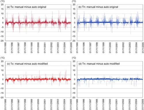
In order to mitigate this incompatibility, hourly dry bulb temperatures from the automated stations were used to find the highest and lowest values recorded for the observing time used at the staffed station. An additional small correction was applied to the highest (lowest) hourly values to simulate continuous measurement of the true daily maximum (minimum). The small correction was approximated by computing average differences among all the archived daily observations and the daily values derived from the hourly values for each automated station; the corrections ranged from 0.2° to 0.6°C for maximum temperature and from -0.2° to -0.4°C for minimum temperature. These corrections were comparable to those produced by Vincent et al. (2009) and Hopkinson et al. (2011). Then, the automated station daily values were modified to match the observing windows, referred to as the modified automated station daily temperature data hereafter. After the modification, the daily values from the staffed stations were in much better agreement, as in the Dawson example (Figs 2c and 2d).

c Auxiliary Data Availability Constrains

Milewska and Hogg (2002) and Guttman and Baker (1996) established that certain meteorological conditions amplify temperature differences at collocated sites on some days and reduce them on other days in a predictable manner as determined by the physical responses of the instrumental and local settings. In this study, it was not possible to explicitly isolate individual instrumental, siting, radiative cooling, ventilation, and insolation biases because all the meteorological elements needed to compute these biases were not observed at these stations. The RCS type of automated station can report hourly wind but not cloud cover. Categorization by wind is usually carried out first, and it alone can improve temperature estimates on specific days at susceptible sites. Categorizing by cloud cover, when available, is secondary within each wind category and could serve as a further refinement.

For example, calm conditions maximize siting bias (local physiography and type of surface under the sensor) and ventilation bias; however, their exact magnitudes cannot be determined because neither the radiative cooling component of the siting bias on clear nights for minimum temperature nor the insolation bias component on clear days for maximum temperature can be further separated due to the lack of cloud reports. Consequently the biases here are identified using the general term “by-wind” based on the element used for categorizing the bias rather than specific names related to its actual origins. The purpose of the paper is to align the old and new temperature series by adjusting persistent biases exposed by meteorological conditions and not to exactly prescribe the source of every bias.

4 Methodology to assess seasonal and seasonal-by-wind biases

The biases associated with seasonal variability and seasonal-by-wind variability are analyzed in this study. As explained in the previous section, further categorizing by cloud cover is not possible because of the unavailability of cloud data at RCSs.

a Categorization of the Data for Calculating Season- and Wind-Dependent Biases

For each day in the overlapping period, the differences between the paired manual and automated (original or modified) observations of daily maximum and minimum temperatures were computed. As a quality control measure, all “manual-minus-automated” differences greater than three standard deviations were excluded from calculations of season- and wind-dependent biases. The exclusion rate was about 1–2%.

Wind speeds were extracted for the hours when the daily maximum and minimum temperatures occurred at the automated station. Instances when the daily temperature difference did not have a matching wind value could arise.

For maximum and minimum temperatures separately, daily “manual-minus-automated” differences were averaged over each of the four seasons to estimate seasonal biases. The seasons were defined as spring (March, April, and May), summer (June, July, and August), fall (September, October, and November), and winter (December, January, and February). Seasonal biases were computed using all available days of data in the season over two different time periods: the first two years and the first five years of the overlapping period.

In addition, within each season, daily differences were grouped according to the following wind speed categories: very light (less than 5 km h⁻¹), light (5 to less than 10 km h⁻¹), moderate (10 to less than 20 km h⁻¹), and strong (20 to 30 km h⁻¹). For each of the four seasons and for each of the four wind categories, daily differences were then averaged to obtain seasonal-by-wind biases. Days with winds greater than 30 km h⁻¹ were ignored for the purpose of bias computation because they were deemed too erratic based on the assessment of the graphs of average biases plotted against all wind values over the entire overlapping series.

b Adjustments at Automated Stations

Adjustments were applied to the daily temperatures of the automated stations (instead of the staffed stations) because hourly temperatures and wind speeds were needed to compute the adjustments, and these observations are always available from automated stations.

For daily maximum (or minimum) temperature, four sets of data were adjusted for seasonal bias or seasonal-by-wind bias based on two-year and five-year overlapping data:

• adjAutoSB2y: adjusted automated stations using the seasonal bias from the two-year overlap,

• adjAutoSB5y: adjusted automated stations using the seasonal bias from the five-year overlap,

• adjAutoSWB2y: adjusted automated stations using the seasonal-by-wind bias from the two-year overlap, and

• adjAutoSWB5y: adjusted automated stations using the seasonal-by-wind bias from the five-year overlap.

For the seasonal-by-wind sets, if the wind was missing for the day or if the count of wind events was fewer than three, then the seasonal bias was used instead of the seasonal-by-wind bias. The event count could be low for strong and very light winds at certain locations. For winds greater than 30 km h⁻¹, the strong wind category bias was used.

Ten years of observations from the start of overlap at each automated station were chosen for the assessment of the results. In order to compare the adjustments for seasonal bias with those for the seasonal-by-wind bias, and for the two-year overlap with those for the five-year overlap, the differences between the adjusted daily temperatures from automated stations and daily temperatures from staffed stations were used over the “trimmed” period of time that excluded the overlap period used to produce the adjustments. This created more stringent conditions for subsequent comparison because the overlap period used to derive the adjustments was not included. The full ten-year time series were also used to compare the adjusted data with the unadjusted data.

In order to assess the results of all the adjustments, eight box-and-whisker plots were produced for each pair of stations for both daily maximum and minimum temperatures. The “adjAutoModOT” are the automated station daily temperatures modified to match the observing time; the following adjusted daily temperatures (“adjAutoSWB2y_full” to “adjAutoSB5y_trimmed”) also include the adjustment to match the observing time. The box plots show the 95th, 75th, median, 25th, and 5th percentiles for the following series of differences (computed as an absolute value):

1. unadjAuto_full minus manual (Unadj),

2. adjAutoModOT_full minus manual (ModOTfu),

3. adjAutoSWB2y_full minus manual (SWB2fu),

4. adjAutoSWB5y_full minus manual (SWB5fu),

5. adjAutoSWB2y_trimmed minus manual (SWB2tr),

6. adjAutoSWB5y_trimmed minus manual (SWB5tr),

7. adjAutoSB2y_trimmed minus manual (SB2tr), and

8. adjAutoSB5y_trimmed minus manual (SB5tr).

Plots 6 and 8 were not computed if the overlap period was less than five years, nor were plots 5 and 7 if the overlap period was less than two years. Plots 3 and 4 were always available, but they could be identical if the overlap period was less than two years because the same length of overlap would have been used in both cases.

To evaluate the different adjustments, the mean absolute differences (MADs) between daily values were also obtained for daily maximum and minimum temperatures separately for the eight scenarios.

5 Results

a Biases Categorized by Season and Wind Conditions

Graphs showing the seasonal biases and the seasonal biases categorized by wind conditions based on the two-year overlap were produced for the daily maximum and minimum temperatures from each of the 22 pairs of stations. For the maximum temperature for Edmonton and Dauphin and the minimum temperature for Edmonton, Dauphin, and Gillam, only the seasonal biases were computed because there were no dry bulb or wind values for the period analyzed. Figure 3 shows four examples of various seasonal biases and seasonal-by-wind biases including counts of events in each classification.

Fig. 3 Examples of biases for (a) daily maximum temperature at Regina; (b) daily maximum temperature at La Ronge; (c) daily minimum temperature at La Ronge; and (d) daily maximum temperature at Tuktoyaktuk. The left panels show the average two-year seasonal-by-wind biases for specific wind categories and the average seasonal biases. The right panels indicate the count of events for the seasonal-by-wind bias and seasonal bias.

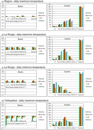
1 Near-zero bias

The maximum temperature at Regina (Fig. 3a), shows near-zero biases, especially in fall and winter. The sites were collocated and had identical elevations (Table 1). Both sites seemed to have similar types of thermistors for temperature measurements, while prevailing moderate-to-strong winds likely ensured good ventilation of the instruments. This example suggests that exact collocation, similar instruments, and a windy climatology can result in minimal biases in the automated observations.

2 Bias dependent on season but not on wind conditions

At La Ronge, both the maximum temperature (Fig. 3b) and the minimum temperature (Fig. 3c) have consistent seasonal patterns. Staffed and automated sites were exactly collocated with no elevation difference, and the staffed site used a thermistor. For the maximum temperature, the positive bias was almost constant, near 0.4°C, throughout the year. For the minimum temperature, the seasonal pattern shows that the summer bias was twice as large as the winter bias (0.4° and 0.2°C, respectively), and the spring and fall biases were approximately 0.3°C. It should also be noted that during the day when the maximum temperature occurs, most winds are moderate while they are very light during the night when the temperature reaches its minimum. Despite many similarities between the manual and the automated sites, certain local settings cause a persistent positive bias between the two stations at this location.

3 Bias dependent on the season and wind conditions

The maximum temperature at Tuktoyaktuk (Fig. 3d) reveals a bias dependent on the season and wind conditions. The negative spring bias differs in magnitude from the other seasons; in addition, it has the greatest value with very light winds and gradually decreases as the winds intensify. Interestingly, other stations situated in the same area around the Beaufort Sea (Paulatuk, Holman, Lupin, and Sachs Harbour) exhibit a similar pattern in spring.

Overall, the results show consistent and reasonably well defined seasonal biases with variable magnitudes at most stations, two-thirds of which also demonstrate some wind dependence. The wind dependence is frequently confined to only one or two seasons, as for the stations in the Beaufort Sea region. The largest biases are also noted in more extreme conditions, either very light or very strong winds, and they are often associated with low occurrence counts.

b Evaluation of the Adjustments

1 Evaluation of the adjustments using Sprague station as an example

Figure 4 shows an example of eight box-and-whisker plots for Sprague, for maximum and minimum temperatures separately, per the numbered list in Section 4.b. All adjusted series, whose performance is summarized in plots 2 to 8, show considerable improvement over the unadjusted series represented in plot 1, as evident from smaller medians and smaller interquartile ranges.

Fig. 4 Box plots showing the 5th, 25th, 50th, 75th, and 95th percentiles of the differences (°C in absolute value) between unadjusted and adjusted observations from automated and staffed stations of (a) daily maximum and (b) daily minimum temperatures at Sprague; the abbreviations along the horizontal axis are explained in Section 4.b.

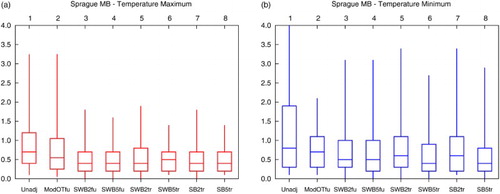
For maximum temperatures (Fig. 4a), the series based on the five-year overlap (SWB5tr and SB5tr) do not outperform the series adjusted using the two-year overlap (SWB2tr and SB2tr). In fact, the magnitude of the improvements, as measured by the medians and interquartile ranges, are very similar in all cases. Looking at the adjusted plots 3 to 8, all medians are 0.3°C smaller than in plot 1 (original plot) except plot 6 in which the median is 0.2°C smaller, and all interquartile ranges are also 0.3°C smaller than in plot 1 except plot 5 in which it is 0.2°C smaller. As expected, plot 2 (ModOTfu) is not much different than plot 1 because the adjustments for different observing times have a much larger effect in central and eastern Canada on minimum temperatures than on maximum temperatures (Vincent et al., 2009). The subsequent adjustments for seasonal bias or seasonal-by-wind bias were more relevant in this case than the observation time adjustment.

For minimum temperatures (Fig. 4b), plots 5 to 8 indicate that time series adjusted using the seasonal-by-wind bias (SWB2tr and SWB5tr) are similar to the respective ones using only seasonal bias (SB2tr and SB5tr). The series adjusted using the five-year overlap (plots 6 and 8) perform better, with their medians being smaller by 0.4°C in relation to plot 1 (original plot), than the series based on the two-year overlap (plots 5 and 7), which have medians smaller by 0.2°C. In addition, the interquartile ranges are also somewhat smaller for the five-year overlap. Plots 3 (SWB2fu) and 4 (SWB5fu) show improvements of a similar magnitude to the other four, with medians closer to zero by 0.3°C and ranges smaller by 0.9° and 0.8°C, respectively. Comparing plot 2 (ModOTfu) with the unadjusted plot 1 clearly demonstrates that adjustments for the different times of observation resulted in the most improvement for the interquartile range by 0.8°C, while the median improved by almost 0.2°C.

2 Comparison of the trimmed series

This comparison is done within the settings that are controlled for the length of overlap and the type of bias. The MADs for all stations for maximum temperature and minimum temperature are summarized in Table 2. The number preceding the name of the adjustment, for example, “5” in 5 SWB2tr, provides the adjustment number used in Table 2 per the numbered list in Section 4.b.

Table 2. Mean Absolute Difference (MAD) between the unadjusted and adjusted maximum and minimum temperatures from automated and staffed stations. The daily temperatures from automated stations 1–13 were modified for the observing time, and the daily temperatures from automated stations 14–23 were not modified for the observing time. Columns 5 to 8 have no values if the overlapping period is shorter than two and/or five years, respectively; columns 9 and 10 have no values if there is no statistically significant shift (at the 0.05 level) detected at the joining date by statistical methods (see Section 6.a). The “*” indicates that only daily maximum temperatures were modified for the observing time for Tuktoyaktuk. The “**” indicates that no wind categorization was applied to either Edmonton or Dauphin maximum or minimum temperatures or to the Gillam minimum temperature: the seasonal bias is substituted for the seasonal-by-wind bias. The results in bold (column 2) give the adjustment for the observing time; the results in italics (columns 3 and 4) give the series for the full period; the results in bold italic (columns 5-8) give the results for the trimmed series.

No.	Location	Prov./Territ.	Maximum Temperature (°C)
			1 Unadj	2 ModObsTfu	3 SWB2fu	4 SWB5fu	5 SWB2tr	6 SWB5tr	7 SB2tr	8 SB5tr	9 MRadj	10 QMadj
1	Princeton	BC	0.7	0.5	0.5	0.5	0.5	0.6	0.5	0.6	0.7	0.8
2	Vernon	BC	0.9	0.8	0.8	0.8	0.9		0.9
3	Creston	BC	0.8	0.8	0.7	0.7	0.7	0.7	0.7	0.7
4	Dawson	YT	1.2	0.8	0.8	0.7	0.8	0.8	0.8	0.8
5	Paulatuk	NT	1.2	0.6	0.7	0.7	0.8	0.7	0.8	0.8
6	Tuktoyaktuk*	NT	1.1	0.5	0.5	0.5	0.5	0.5	0.5	0.6
7	Lupin	NU	1.2	0.8	0.6	0.6	0.6	0.7	0.6	0.7
8	Holman	NT	1.1	0.7	0.8	0.7	0.9	0.9	0.9	0.9
9	Sachs Harbour	NT	1.0	0.7	1.2	0.6	1.3	0.6	1.1	0.6
10	Lacombe	AB	0.8	0.6	0.6	0.6
11	Sprague	MB	1.0	0.8	0.6	0.6	0.6	0.6	0.6	0.5	0.9	0.9
12	Kapuskasing	ON	1.1	0.8	0.4	0.4					0.9	0.9
13	Ottawa	ON	0.5	0.4	0.4	0.3	0.4	0.3	0.4	0.3	0.5	0.5
14	Tuktoyaktuk*	NT
15	Edmonton**	AB	0.4		0.3	0.2	0.3	0.2	0.3	0.3	0.3	0.3
16	Beaverlodge	AB	0.5		0.5	0.5	0.5		0.5
17	Moose Jaw	SK	0.4		0.4	0.4
18	Regina	SK	0.2		0.2	0.2	0.2	0.2	0.2	0.2
19	La Ronge	SK	0.4		0.2	0.2	0.2	0.3	0.2	0.3	0.4	0.4
20	Dauphin**	MB	0.1		0.1	0.1	0.1	0.2	0.1	0.2	0.4	0.4
21	Gillam**	MB	0.4		0.3	0.3	0.3	0.3	0.3	0.3
22	Thunder Bay	ON	0.2		0.2	0.2
23	Gander	NL	0.4		0.4	0.4	0.3	0.3	0.3	0.3
			Minimum Temperature (°C)
No.	Location	Prov./Territ.	1 Unadj	2 ModObsTfu	3 SWB2fu	4 SWB5fu	5 SWB2tr	6 SWB5tr	7 SB2tr	8 SB5tr	9 MRadj	10 QMadj
1	Princeton	BC	0.7	0.4	0.3	0.3	0.3	0.3	0.3	0.3	0.7	0.7
2	Vernon	BC	2.6	2.6	1.2	1.1	1.2		1.2		2.0	2.2
3	Creston	BC	1.1	1.1	1.0	1.0	1.0	1.0	1.0	1.0	1.0	1.0
4	Dawson	YT	1.0	0.7	0.5	0.5	0.5	0.5	0.5	0.5
5	Paulatuk	NT	1.2	0.7	0.6	0.6	0.7	0.7	0.6	0.7
6	Tuktoyaktuk*	NT
7	Lupin	NU	1.3	0.9	0.7	0.7	0.7	0.8	0.7	0.8
8	Holman	NT	1.0	0.7	0.8	0.7	0.8	0.9	0.8	0.9
9	Sachs Harbour	NT	1.2	0.8	0.9	0.8	0.9	0.8	0.9	0.8
10	Lacombe	AB	1.2	0.8	0.8	0.8					1.4	1.4
11	Sprague	MB	1.5	0.9	0.9	0.9	1.0	0.8	1.0	0.8	1.4	1.5
12	Kapuskasing	ON	1.6	0.9	0.4	0.4					1.9	1.9
13	Ottawa	ON	0.9	0.3	0.3	0.3	0.3	0.4	0.3	0.4	1.0	1.0
14	Tuktoyaktuk*	NT	0.5		0.5	0.5	0.5	0.6	0.5	0.6
15	Edmonton**	AB	0.2		0.2	0.2	0.2	0.2	0.2	0.2
16	Beaverlodge	AB	0.4		0.4	0.4	0.4		0.4		0.5	0.5
17	Moose Jaw	SK	0.6		0.6	0.6					1.0	0.8
18	Regina	SK	0.2		0.2	0.2	0.2	0.2	0.2	0.2	0.7	0.8
19	La Ronge	SK	0.3		0.3	0.2	0.3	0.3	0.3	0.3
20	Dauphin**	MB	0.2		0.2	0.2	0.2	0.2	0.2	0.2	0.5	0.5
21	Gillam**	MB	0.4		0.4	0.4	0.4	0.5	0.4	0.4
22	Thunder Bay	ON	0.3		0.2	0.2
23	Gander	NL	0.6		0.6	0.5	0.3	0.3	0.3	0.2

i Comparison of automated stations adjusted using seasonal-by-wind bias and seasonal bias

In order to determine whether the inclusion of the wind improved the adjustments, the seasonal-by-wind adjusted series (5 SWB2tr and 6 SWB5tr) are compared with their respective series (7 SB2tr and 8 SB5tr) adjusted using the seasonal bias. The results for Edmonton and Dauphin for both maximum and minimum temperatures and Gillam for minimum temperature are all based on seasonal biases because the algorithm automatically substituted with these biases for all missing winds during the period, and thus should be excluded from this comparison. The results in Table 2 indicate that the adjustments that include categorization by winds did not further improve the overall statistics compared with the seasonal adjustments for this particular set of stations because all the MADs are similar (within 0.1°C). Because these stations show limited wind dependence, it is expected that the small number of days affected by wind do not influence the overall MADs. This is examined further in Section 5.b.4

ii Comparison of automated stations adjusted using two-year and five-year overlap

In order to determine whether using five years of overlapping data improves the adjustments, the series 5 SWB2tr and 7 SB2tr adjusted using 2-year overlapping data are compared with their respective series 6 SWB5tr and 8 SB5tr adjusted using five-year overlapping data. The results indicate that using five years instead of two years of overlapping data did not improve the adjustments for this particular set of stations. The exception was the minimum temperatures from Sprague where the MAD is reduced from 1.0°C using the two-year data to 0.8°C using the five-year data for both the seasonal-by-wind bias and seasonal bias. Another case is Sachs Harbour that has some missing data at the beginning of the period; this obviously affects the adjustments based on the two-year overlapping data more than those based on the five-year overlapping data.

3 Comparison of the full series

When adjusted time series 3 SWB2fu are compared with 4 SWB5fu, the findings of Section 5.b.2 are supported. Hereafter, series 3 SWB2fu is chosen to further evaluate the overlap methodology because the two-year overlapping period has been used the most frequently in the typical operational settings of climate monitoring.

i Automated stations modified to match observing time

When the adjusted series 3 SWB2fu are compared with the unadjusted series 1 Unadj, the MADs, medians, and interquartile ranges all indicate improvement with adjustments for the 13 automated stations modified for the observing time (first 13 stations listed in Table 2 for either maximum temperature or minimum temperature). The MADs are generally smaller by 0.1° to 0.7°C for maximum temperature and by 0.1° to 1.4°C for minimum temperature. Most of this improvement can be attributed to the modification of the observing time because the MADs from 3 SWB2fu are similar to those from 2 ModOTfu. By comparing 3 with 2 in Table 2, it is evident that the impact of the adjustment for seasonal-by-wind biases alone is minor, generally around 0° to 0.1°C, with a few values being higher in each series.

The medians (not shown) generally demonstrate an improvement of 0.1° to 0.4°C for maximum temperatures and 0.2° to 1.5°C for minimum temperatures. The interquartile ranges also display substantial improvement; the ranges are reduced by 0.1° to 0.6°C for the maximum temperature and by 0.2° to 1.0°C for minimum temperature.

ii Automated stations not modified to match the observing time

For the last ten stations listed in Table 2 for either maximum temperature or minimum temperature, most of the MADs for 3 SWB2fu are identical to the unadjusted dataset 1 Unadj, in a few cases they are smaller by 0.1°C, and La Ronge maximum temperature is smaller by 0.2°C. The medians and interquartile ranges (not shown) are identical or within 0.1°C with two exceptions. The first is Moose Jaw, with the median for the minimum temperature worse by −0.4°C as a result of the short overlapping period of six months during summer and fall only; however, its interquartile range still improves by 0.4°C. The second is La Ronge, which shows an improvement of 0.2°C for maximum temperature in both statistical parameters.

4 Comparison of the series adjusted for seasonal bias and seasonal-by-wind bias in wind-dependent cases

In this section, the seasonal bias and seasonal-by-wind bias are compared for the stations affected by the wind bias.

Four stations that showed strong wind dependence are listed in Table 3. The largest seasonal-by-wind bias occurs for the maximum temperature in spring, in light winds in Paulatuk, Tuktoyaktuk, and Holman and in strong winds in Creston. All spring days with the appropriate wind conditions were extracted from the full period. For the selected days, MADs were computed between the daily temperatures at the conventional stations and three series of daily temperatures from the automated stations: (i) modified for the observing time; (ii) modified and adjusted for the seasonal bias; and (iii) modified and adjusted for seasonal-by-wind bias. Table 3 shows that for the first three stations MADs are smaller for case (ii) than for case (i), and MADs for case (iii) are smaller than for case (ii). Holman, the only station with poorer results, was investigated further. It was determined that there was an obvious change at that station after the first two-year overlapping period because negative spring differences were no longer present.

Table 3. MADs between conventional and automated stations for days adjusted by largest wind biases at select stations with well-defined wind dependence.

Location	Largest Spring Bias Based on 2-year Overlap (°C)	Spring Wind Category for Maximum Temperatures	Count (days)	MAD (°C)
				ModOTfu	SB2fu	SWB2fu
Creston	0.9	strong	83	0.94	0.69	0.54
Paulatuk	−1.5	very light	137	1.51	1.19	1.16
Tuktoyaktuk	−1.6	very light	103	1.45	0.91	0.71
Holman	−1.0	very light	194	1.36	1.52	1.73

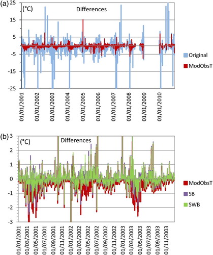
Actual differences after each adjustment are illustrated for Tuktoyaktuk; Fig. 3d shows that all biases are negative with strong wind dependence in spring and weak in other seasons. Figure 5a shows two plots of all the daily maximum temperatures differences computed between the conventional and the original reports from the automated stations, as well as between the reports from the conventional and after the automated stations had been modified for observing time. The time-modified differences are much smaller than the original and show cyclical large negative differences every spring. Figure 5b is an enlargement of these modified differences; only the first three years are presented for readability. Two more series of differences are added for comparison—between the conventional daily temperatures and the temperatures from the automated station that were adjusted for seasonal bias and seasonal-by-wind bias. These plots clearly show additional progressive reductions in the differences when the series are adjusted for seasonal bias and seasonal-by-wind bias, the largest occurring in spring. After the final adjustment, the series of differences for seasonal-by-wind bias resemble random noise because the portions of the differences that can be explained by physical conditions have been eliminated.

Fig. 5 Differences in daily maximum temperature between the conventional station and automated station at Tuktoyaktuk: (a) between original daily values (blue) and after modification for the observing time at the automated station (red) and (b) after modification for the observing time at the automated station (red); as well as after it was adjusted for seasonality (purple) and both seasonality and wind dependence (green).

6 Discussion and summary

a Comparison of Overlap and Neighbour-based Adjustments

Overlapping observations were rarely collected in the past, thus statistical methods used data from neighbouring stations to infer adjustments to account for discontinuities resulting from changes in instrumentation, observing procedures, or location. In this section, adjustments derived from overlapping observations are compared with those based on neighbouring stations. These latter are obtained using the homogenization procedures that were applied to prepare the first and second versions of the homogenized daily temperatures in Canada (see Section 2.c).

Observations from staffed and automated stations were joined to create a single time series. For example, if data from staffed stations ended in 1999 and data from automated stations started in 1995, then the automated observations were joined with the manual observations in 1995. Regression models (Vincent et al., 2012) were applied to the year–month time series of the tested series with the use of three to ten neighbouring stations separately in order to determine if there had been a statistically significant shift (at the 0.05 level) at the joining date. If there had been no significant shift then no adjustments were produced. In the case of a significant shift, two methods were used to obtain daily adjustments: the MR procedure (Vincent et al., 2002) and the QM algorithm (Wang, Feng, & Vincent, 2014).

The differences between the series for the automated and staffed stations adjusted by MR and QM were computed and the results are presented in Table 2 (columns 9 and 10, respectively). The method did not detect a significant shift at the joining date when neighbouring stations were located far from the tested station. This is the case for the six stations in the North (Dawson, Paulatuk, Tuktoyaktuk, Lupin, Holman, and Sachs Harbour), whose nearest neighbour was more than 300 km from the test site, and for the three isolated stations (Gilliam, Thunder Bay, and Gander), whose closest neighbour was more than 100 km away. For the remaining stations, the neighbours were relatively near the test site (<100 km), and the correlation between the daily data and the first difference series is relatively good (>0.7). For these remaining 13 stations (or 26 remaining situations because daily maximum and minimum temperatures were assessed separately), there are eight situations with no significant shift detected at the joining date (Creston's maximum temperatures, for example); the shift could have been too small compared with the data variability. There are 13 situations with a significant shift detected, but the MR and QM adjustments did not reduce the MAD between the adjusted automated and staffed stations (Lacombe's minimum temperatures, for example); in some of these situations, it is possible that adjustments for different observing times are needed first. Finally, there are five situations for which the MR and QM adjustments reduced the MAD (Vernon's minimum temperatures, for example).

This preliminary study first indicates that it is preferable to align daily temperature observations from staffed stations to automated stations using overlapping data if available (the MAD in columns 9 and 10 are larger or equal to those in columns 2 to 8 for the automated stations modified to match the observing time). The results also show that adjustments based solely on procedures without using the overlapping data can create a greater difference between the adjusted manual and automated data (the MAD in columns 9 and 10 can be greater than or equal to those in column 1). Consequently, adjustments based solely on neighbouring stations do not necessarily resolve the bias between staffed and automated sites. Further work is required to assess statistical adjustments, similar to those produced by the MR and QM procedures, using simulated daily temperatures and overlapping data to determine the limitations of these procedures.

b Conclusions and Recommendations

The inception and development of the Reference Climate Network in Canada, as well as its modernization from the 1990s to the early 2000s has been described. Concurrent overlapping observations from conventional stations and the new Campbell Scientific automated stations with a standardized configuration were examined at 22 locations for the purpose of preserving the continuity of long-term climate records. First, the observing windows for the daily maximum and minimum temperatures were matched for some of the pairs of stations. Second, biases based on meteorological conditions, in particular the season and wind speed, were computed and then used to adjust the time series of observations from the automated stations. Further categorization by cloud cover was not possible because clouds were not observed by the Campbell Scientific automated stations, and sky condition observations at staffed stations were limited to airports, and, in recent years, often to daytime hours only.

Two- and five-year overlapping periods were selected to develop seasonal biases, which were further categorized by wind speed in order to determine whether inclusion of wind conditions improved the results.

Almost all maximum and minimum temperature biases varied with season, sometimes only by a small amount; some biases also varied with wind speed. The more pronounced wind dependence was usually confined to one season and the largest magnitudes were limited to a relatively small number of days in a specific wind category, usually the lightest winds.

Time series adjusted using two- and five-year overlapping data were similar. The lack of dependence on the length of the overlap supported the stationarity postulation (i.e., climatological conditions changed little from year to year, and the biases remained stable and valid over several years). It is encouraging that the biases seemed to be stable regardless of the two- or five-year length of the overlap, but their continued validity may need to be re-evaluated periodically.

In comparison with the original series, the time series for automated stations adjusted for seasonal-by-wind bias showed great improvement for the set of 13 stations that had their daily maximum and minimum temperatures modified to match the observing windows at the staffed station. Smaller MADs between the paired stations, up to 0.7°C and 1.4°C, for the maximum temperature and minimum temperature, respectively, were found. Most of the improvement was attributed to aligning the time of observation, which improved MADs by up to 0.7°C. The adjustment did not make much difference in the second group of nine stations, which originally had the same observing windows and smaller initial MADs of unadjusted series of approximately 0.5°C or less.

It was not obvious whether any the use of the liquid-in-glass thermometers at seven conventional stations caused any bias. Even though five of these stations had average biases greater than 0.4°C for either maximum or minimum temperatures adjusted for seasonal-by-wind bias, they also had non-zero separation distances and/or non-zero elevation differences. Each station in the field has a unique combination of influencing factors that amplify or cancel each other. This is not a prearranged side-by-side study where all elements are controlled and can be changed and analyzed separately. Leeper, Rennie, and Palecki (2015) also noted that, in contrast to the side-by-side comparisons, the mean differences between stations in networks are highly variable and unrelated to sensing technology used at staffed volunteer climate stations (liquid-in-glass or digital) or even station separation but rather to local geographic and siting factors.

Following these findings, the main recommendation from this study is the need to continually verify the compatibility of the observing window, either from the available station information metadata or by using the hourly dry bulb temperatures as described in this paper, first to confirm the observing time at the station then, if required, to match the observing time to the other station in the pair. Another option, which has only become available since 2014 under the new archived Data Management System, is to use new synoptic six-hourly and hourly maximum and minimum temperatures from the Campbell Scientific automated stations; this would allow ease and flexibility in almost effortlessly deriving daily maximum and minimum temperatures for any observing window. As explained by Whitfield (2012), the user always needs to assess whether the environmental data fit the purpose and whether any adjustments are required.

It is recommended that network managers make every possible effort to cover all four seasons with overlapping observations and gather a sufficient number of events for all relevant meteorological conditions. The gathering of overlapping observations may need to be repeated periodically when warranted by considerable changes in the environment, station settings, instrumentation, or monitoring procedures.

Automation of the network is ongoing and, in the case of temperature, does not have to be a hindrance when managed appropriately. In fact, Fiebrich and Crawford (2009) suggested that automation of temperature observations can actually result in overall improvement in the quality of records. After comparing overlapping records, they showed that automated stations from the Oklahoma Mesonet, and indirectly USCRN, produced much more stable and consistent observations, whereas USHCN stations, often assumed by scientists to be of superior quality, had numerous large errors that could be linked to the behaviour of the observer, for example, incorrect date archived, data routinely date shifted, incorrect resets of sensors, late or early observations, and transcription errors. Trewin (2010) also saw small overall biases with automation and new temperature sensors, with any differences being due to location; when he later performed an evaluation of automation he did not see any substantial inhomogeneities where the manual and automated instruments were collocated in the same Stevenson screen or in different screens about 3 m apart (Trewin, 2012). Even when the change eventually results in more complete, consistent, and reliable temperature datasets from the automated stations, the issue is the change itself. Having overlapping data is very helpful in managing this change appropriately for the purpose of the computation of long-term trends.

As anticipated, the approach based on overlapping records produced better results than statistical methods using neighbouring stations for all the stations, both modified and unmodified for the observing times. As far as compatibility of the observing windows, it appears that both MR and QM procedures could benefit from aligning observing times, where possible, before proceeding with the actual step detection and adjustment. In the future, as awareness and recognition of the benefits of collecting overlapping observations increase and the practice becomes widespread in climate network management, the use of overlapping records to correct discontinuities should expand in any approach, either using meteorological conditions as in this paper or by adapting them in various statistical methods.

Acknowledgements

We would like to thank our colleagues Xiaolan Wang and Hui Wan from the Climate Research Division of Environment Canada and two reviewers for their helpful comments and suggestions for this manuscript.

Disclosure statement

No potential conflict of interest was reported by the authors.

References

- Atmospheric Environment Service. (1991). World Meteorological Organization reference climatological stations, Canada, Version 2.5 (Internal Report). Atmospheric Environment Service, Downsview, Ontario, Canada.
- Atmospheric Environment Service. (1993). Historical Canadian Climate Database, Canadian climate stations selected for analysis of current and historical regional and national air temperature trends, variations and anomalies (Internal Report). Atmospheric Environment Service, Downsview, Ontario, Canada.
- Baker, C. B., & Helfert, M. R. (2008). U.S. Climate Reference Network (USCRN): A unique national long-term climate monitoring network. 12th Conf. on IOAS-AOLS 9 (Integrated Observing and Assimilation Systems for the Atmosphere, Oceans and Land Surface), New Orleans, LA, Amer. Meteor. Soc. Retrieved from https://ams.confex.com/ams/88Annual/webprogram/Paper130984.html
- Changnon, S. A., & Kunkel, K. E. (2006). Changes in instruments and sites affecting historical weather records: A case study. Journal of Atmospheric and Oceanic Technology, 23, 825–828. doi: 10.1175/JTECH1888.1
- Davey, C. A., & Pielke, R. A., Sr. (2005). Microclimate exposures of surface-based weather stations. Bulletin of the American Meteorological Society, 86, 497–504. doi: 10.1175/BAMS-86-4-497
- Della-Marta, P., & Wanner, H. (2006). A method of homogenizing the extremes and mean daily temperature measurements. Journal of Climate, 19, 4179–4197. doi: 10.1175/JCLI3855.1
- Diamond, H. J., Karl, T. R., Palecki, M. A., B. Baker, C., Bell, J. E., Leeper, R. D., … Thorne, P. W. (2013). U.S. Climate Reference Network after one decade of operations: Status and assessment. Bulletin of the American Meteorological Society, 94, 485–498. doi:10.1175/BAMS-D-12-00170.1
- Environment Canada. (1996). Climate network rationalization (Report of working group). Downsview, Ontario: Atmospheric Environment Service.
- Environment Canada. (cited 2012). Weather Station Swap. EnviroZine Environment Canada's Online Newsmagazine, No. 88.
- Fiebrich, C. A., & Crawford, K. C. (2009). Automation: A step toward improving the equality of daily temperature data produced by climate observing networks. Journal of Atmospheric and Oceanic Technology, 26, 1246–1260. doi: 10.1175/2009JTECHA1241.1
- Gallo, K. P. (2005). Evaluation of temperature differences for paired stations of the U. S. Climate Reference Network. Journal of Climate, Notes and Correspondence, 18, 1629–1636. doi: 10.1175/JCLI3358.1
- Goodrich, D., & Westermeyer, W. (cited 2012). The global climate observing system – 20th Anniversary. World Meteorological Organization Bulletin, 61(1), 3–7.
- Gullett, D. W., Louie, P. Y. T., & Milewska, E. (1995). Future climate monitoring and historical climate data requirements for the Climate Research Branch (Internal Report). Atmospheric Environment Service, Downsview, Ontario, Canada.
- Guttman, N. B., & Baker, C. B. (1996). Exploratory analysis of the difference between temperature observations recorded by ASOS and conventional methods. Bulletin of the American Meteorological Society, 77(12): 2865–2873. doi: 10.1175/1520-0477(1996)077<2865:EAOTDB>2.0.CO;2
- Hopkinson, R. F., McKenney, D. W., Milewska, E. J., Hutchinson, M. F., Papadopol, P., & Vincent, L. A. (2011). Impact of aligning climatological day on gridding daily maximum–minimum temperature and precipitation over Canada. Journal of Applied Meteorology and Climatology, 50, 1654–1665. doi: 10.1175/2011JAMC2684.1
- Hubbard, K. G., & Lin, X. (2006). Reexamination of instrument change effects in the U. S. Historical Climatology Network. Geophysical Research Letters, 33, L15710, 1–4. doi:10.1029/2006GL027069
- Hubbard, K. G., Lin, X., & Baker, C. B. (2005). On the USCRN temperature system. Journal of Atmospheric and Oceanic Technology, 22, 1095–1100. Notes and Correspondence. doi: 10.1175/JTECH1715.1
- Hubbard, K. G., Lin, X., Baker, C. B., & Sun, B. (2004). Air temperature comparison between the MMTS and the USCRN temperature systems. Journal of Atmospheric and Oceanic Technology, 21, 1590–1597. doi: 10.1175/1520-0426(2004)021<1590:ATCBTM>2.0.CO;2
- Leeper, R. D., Rennie, J., & Palecki, M. A. (2015). Observational perspectives from U.S. Climate Reference Network (USCRN) and Cooperative Observer Program (COOP) Network: Temperature and precipitation comparison. Journal of Atmospheric and Oceanic Technology, 32, 703–721. doi:10.1175/JTECH-D-14-00172.1
- McKee, T. B., Doesken, N. J., Davey, C. A., & Pielke, R. A., Sr. (2000). Climate data continuity with ASOS. Climatology Report No. 00-3 for April 1996 through June 2000, Colorado Climate Center, Department of Atmospheric Science, Colorado State University, Fort Collins, Colorado.
- Mestre, O., Gruber, C., Prieur, C., Caussinus, H., & Jourdain, S. (2011). SPLIDHOM: A method for homogenization of daily temperature observations. Journal of Applied Meteorology and Climatology, 50, 2343–2358. doi: 10.1175/2011JAMC2641.1
- Meteorological Branch, Department of Transport. (1966). List of reference climatological stations in Canada, DS # 20-66. Downsview, Ontario.
- Milewska, E., & Hogg, W. D. (2001). Spatial representativeness of a long-term climate network in Canada. Atmosphere-Ocean, 39(2), 145–161. doi: 10.1080/07055900.2001.9649671
- Milewska, E., & Hogg, W. D. (2002). Continuity of climatological observations with automation. Atmosphere-Ocean, 40(3), 333–359. doi: 10.3137/ao.400304
- NOAA. (2011). US Climate Reference Network. Annual report for FY 2011 – October 2011, National Oceanic and Atmospheric Administration, Boulder, Colorado: National Climate Data Center. Retrieved from http://www1.ncdc.noaa.gov/pub/data/uscrn/publications/annual_reports/FY11_USCRN_Annual_Report.pdf
- NOAA. (2012). The USHCN Version 2 Serial Monthly Datasets. National Oceanic and Atmospheric Administration, National Climatic Data Center. Retrieved from http://www.ncdc.noaa.gov/oa/climate/research/ushcn/#biasadj
- Schrumpf, A. D., & McKee, T. B. (1996). Temperature data continuity with the automated surface observing system. Atmospheric Science Paper No. 616, Climatology Report Number 96-2, Department of Atmospheric Science, Colorado State University, Fort Collins, Colorado.
- Sun, B., Baker, C. B., Karl, T. R., & Gifford, M. D. (2005). A comparative study of AOS and USCRN temperature measurements. Journal of Atmospheric and Oceanic Technology, 22, 679–686. doi: 10.1175/JTECH1752.1
- Trewin, B. (2010). Exposure, instrumentation, and observing practice effects on land temperature measurements. Wiley Interdisciplinary Reviews: Climate Change, 1(4), 490–506. doi:10.1002/wcc.46
- Trewin, B. (2012). A daily homogenized temperature data set for Australia. International Journal of Climatology, 33 (6), 1510–1529. doi: 10.1002/joc.3530
- Trewin, B. C., & Trevitt, A. C. F. (1996). The development of composite temperature records. International Journal of Climatology, 16, 1227–1242. doi: 10.1002/(SICI)1097-0088(199611)16:11<1227::AID-JOC82>3.0.CO;2-P
- Vincent, L. A., Milewska, E. J., Hopkinson, R. F., & Malone, L. (2009). Bias in minimum temperature introduced by a redefinition of the climatological day at the Canadian synoptic stations. Journal of Applied Meteorology Climatology, 48, 2160–2168. doi: 10.1175/2009JAMC2191.1
- Vincent, L. A., Wang, X. L., Milewska, E. J., Wan, H., Yang, F., & Swail, V. (2012). A second generation of homogenized Canadian monthly surface air temperature for climate trend analysis. Journal of Geophysical Research, 117, D18110, 1–18. doi:10.1029/2012JD017859.
- Vincent, L. A., Zhang, X., Bonsal, B. R., & Hogg, W. D. (2002). Homogenization of daily temperatures over Canada. Journal of Climate, 15, 1322–1334. doi: 10.1175/1520-0442(2002)015<1322:HODTOC>2.0.CO;2
- Wang, X. L., Chen, H., Wu, Y., Feng, Y., & Pu, Q. (2010). New techniques for the detection and adjustment of shifts in daily precipitation data series. Journal of Applied Meteorology and Climatology, 49, 2416–2436. doi:10.1175/2010JAMC2376.1
- Wang, X. L., Feng, Y., & Vincent, L. A. (2014). Observed changes in one-in-20 year extremes of Canadian surface air temperatures. Atmosphere-Ocean, 52(3), 222–231. doi: 10.1080/07055900.2013.818526
- Whitfield, P. H. (2012). Why the provenance of data matters: Assessing “Fitness for Purpose” for environmental data. Canadian Water Resources Journal, 37(1): 23–36. doi: 10.4296/cwrj3701866
- WMO. (1966). Climatic change, Technical Note No. 79, Report of a Working Group of the Commission for Climatology. World Meteorological Organization, WMO - No. 195. TP. 100, Geneva, Switzerland.
- WMO. (1986). Guidelines on the selection of Reference Climatological Stations (RCSs) from the existing climatological station network. World Meteorological Organization, World Climate Programme series, WCP-116, WMO/TD-No. 130, Geneva, Switzerland.
- WMO. (1993). Report of the experts meeting on Reference Climatological Stations (RCS) and National Climate Data Catalogues (NCC). World Meteorological Organization, World Climate Data and Monitoring Programme series, WCDMP-No. 23, WMO-TD No. 535, Offenbach am Main, Germany.
- WMO. (2007). Guidelines for managing changes in climate observation programmes. World Meteorological Organization, World Climate Data and Monitoring Programme series, WCDMP-No. 62, WMO-TD No. 1378, Geneva, Switzerland.