On Measurements of the Tide at Churchill, Hudson Bay

Abstract

Since the late 1990s the semi-diurnal tide at Churchill, on the western shore of Hudson Bay, has been decreasing in amplitude, with M₂ amplitudes falling from approximately 154 cm in 1998 to 146 cm in 2012 and 142 cm in 2014. There has been a corresponding small increase in phase lag. Mean low water, decreasing throughout most of the twentieth century, has levelled off. Although the tidal changes could reflect merely a malfunctioning tide gauge, the fact that there are no other measurements in the region and the possibility that the tide is revealing important environmental changes calls for serious investigation. Satellite altimeter measurements of the tide in Hudson Bay are complicated by the seasonal ice cover; at most locations less than 40% of satellite passes return valid ocean heights and even those can be impacted by errors from sea ice. Because the combined TOPEX/Poseidon, Jason-1, and Jason-2 time series is more than 23 years long, it is now possible to obtain sufficient data at crossover locations near Churchill to search for tidal changes. The satellites sense no changes in M₂ that are comparable to the changes seen at the Churchill gauge. The changes appear to be localized to the harbour, or to the Churchill River, or to the gauge itself.

Résumé

[Traduit par la rédaction] L'amplitude de la marée semi-diurne diminue depuis la fin des années 1990 à Churchill, sur la côte ouest de la baie d'Hudson. L'amplitude de la composante M₂ s’élevait à environ 154 cm en 1998. Elle a chuté à 146 cm en 2012 et à 142 cm en 2014. Une légère augmentation du déphasage s'est aussi produite. Le niveau de la basse mer moyenne, en baisse durant la majeure partie du XX^e siècle, s'est stabilisé. Bien que ces modifications de la marée aient pu être attribuées à un mauvais fonctionnement du marégraphe, il reste qu'aucune autre mesure n'existe pour la région. La possibilité que la marée nous révèle d'importants changements environnementaux nous force à prendre le problème au sérieux. Le couvert de glace saisonnier complique la prise de mesures altimétriques par satellite de la marée dans la baie d'Hudson. Pour la plupart des sites, moins de 40 % des passages de satellites fournissent des hauteurs marines valides, et même celles-ci peuvent être minées par les erreurs que cause la glace de mer. Comme la série temporelle combinée issue de TOPEX/Poseidon, de Jason-1 et de Jason-2 s’étend sur plus de 23 ans, il est maintenant possible d'effectuer des recoupements avec des sites près de Churchill afin d’étudier les changements dans la marée. Les satellites ne détectent pas de changements de la composante M₂ qui seraient comparables à ceux des relevés du marégraphe de Churchill. Ces changements semblent se confiner au port ou à la rivière Churchill, ou encore à la station marégraphique même.

KEYWORDS:

• tides
• tidal changes
• tide gauges
• satellite altimetry

1 Introduction

The semi-diurnal tide in Hudson Bay is known to experience large seasonal changes in amplitude and phase in response to seasonal changes in ice cover (Godin, 1986; Prinsenberg, 1988; St- Laurent, Saucier, & Dumais, 2008). Along the western boundary where the tidal amplitudes are largest and exceed 1.5 m, the seasonal changes in M₂ are of order 10 cm in amplitude and 10° in phase, among the most notable anywhere in the world. Numerical modelling (St-Laurent, Saucier, & Dumais, 2008) shows that the frictional increase from overlying ice in Foxe Basin (north of Hudson Bay and connected via Hudson Strait and a few smaller channels) has the greatest impact on tidal changes throughout the whole system (i.e., the tidal changes at any one location may be induced by rather distant dissipational changes from varying ice cover).

In addition to the large seasonal cycle, the amplitude of M₂ as measured at the tide gauge at Churchill, Manitoba, has in recent years been undergoing a marked decline along with a slightly increasing phase lag — see Section 2 below. Could this change be related to climatic changes in ice cover? It is known that sea ice in Hudson Bay, like that throughout most of the Arctic Ocean, is experiencing a secular decline (Cavalieri & Parkinson, 2012), although with a trend of approximately −6% per decade, the change over one decade is admittedly much smaller than changes associated with the seasonal cycle. Or is the tidal trend at Churchill a more local phenomenon, possibly related to hydrology of the Churchill River — the gauge sits in the mouth of the river — or is it merely an instrument malfunction?

The latter is sufficiently common in tide-gauge measurements, especially those undertaken in harsh conditions, that it is ill-advised to accept unusual measurements unless they can be corroborated by nearby measurements. Unfortunately, the gauge at Churchill is the only permanently operating gauge in Hudson Bay. An alternative is to examine the Hudson Bay tide by remote sensing, but the use of satellite altimetry in this region is challenging; the only valid ocean data are obtained in summer ice-free conditions, and in fact far less than half the satellite overflights of TOPEX/Poseidon (T/P) yield useful data. It is only now, after 23 years of combined measurements from the T/P, Jason-1, and Jason-2 satellites, that it is marginally possible to obtain the precision necessary to investigate tidal changes. As shown below, the altimetry suggests that the large decadal change in the tide at Churchill is not occurring in the more open expanses of western Hudson Bay.

Section 2 consists of an analysis of the tide at Churchill, obtained from hourly measurements collected from 1940 to 2014 by the Canadian Hydrographic Service. Section 3 turns to an analysis of satellite altimetry over the 1992–2014 time frame. The most dramatic changes at Churchill occur in the largest constituent, M₂, so most attention is focused on it. This is necessarily so for the satellite analyses because the precision of smaller constituents is probably inadequate for detecting change.

2 Analysis of Churchill tide

To determine a precise and fairly complete view of the tidal constants at Churchill and to help guide subsequent analyses of yearly data, an initial high-resolution harmonic analysis was computed for the period 1968 through 1999. A set of 97 constituents was found to eliminate most of the isolated lines in the residual spectrum, leaving broad cusps (Munk, Zetler, & Groves, 1965) in the semi-diurnal, quarter-diurnal and sixth-diurnal species, but hardly any in the odd-diurnal bands. Such cusps are anticipated in light of the tidal variability described above.

The tide at Churchill is predominantly semi-diurnal, with the mean amplitude of M₂ over the thirty years of the analysis equal to 154.6 cm. Diurnal constituents are small: K₁ is 8.5 cm and O₁ is only 3.6 cm. The semi-diurnal admittance amplitude is very comparable at the frequencies of 2N₂, N₂, and M₂, but it falls off by more than 30% at the higher frequencies of S₂ and K₂; the phase lags increase almost monotonically with frequency across the band, advancing roughly 40° between each tidal group.

Because of the importance of M₂ and its variability, special attention must be given to spectral lines within and near the M₂ group. The strong seasonal variability induces 1 cpy (cycle per year) sidelines around M₂, which are often denoted MA₂ and MB₂, or possibly α₂ and β₂, and these are indeed relatively large: 6.2 and 4.7 cm, respectively. Given that the seasonal changes in M₂ are not purely sinusoidal (Godin, 1988, see also below), lines at 2 cpy from M₂ might also be expected, but such lines would overlap the compound tides MSK₂ and MKS₂, which are already included in the 97-constituent set. The tide MSK₂ is also relatively large, with amplitude 2.3 cm. It is close in frequency to the gravitational constituent , but the latter turns out almost an order of magnitude smaller and thus need not be included in a yearly analysis; note that these two frequencies cannot be separated except in a multi-year analysis. Table 1 summarizes all these lines that fall within the M₂ tidal group. Although the time series is certainly sufficiently long to solve for nodal sidelines, this is unnecessary for the purposes at hand, so standard nodal corrections (updated daily) were used.

Table 1. Estimated amplitudes and phases for lines in the M₂ Group.^a

Tide	Doodson No.	ω (° h^−1)	Amp. (cm)	Phase lag (°)
MSK2	253.555	28.901967	2.34	222.7
	253.755	28.911251	0.35	39.9
MA2	254.555	28.943036	6.18	283.1
M2	255.555	28.984104	154.63	25.1
MB2	256.555	29.025173	4.71	270.7
MKS2	257.555	29.066242	0.97	293.7

^aEstimated from the Churchill tide gauge data for years 1968–1999. Phase lags are with respect to the Greenwich meridian. Based on the residual cusp surrounding the M₂ group, the standard error for all these lines is approximately 0.43 cm.

The spectrum of residuals revealed the need for similar terms around N₂; the International Hydrographic Organization (IHO, 2006) already anticipates this requirement with a notation similar to that used for M₂, namely NA₂ and NB₂. Similar line splitting at S₂ is automatically incorporated through the gravitational constituents R₂ and T₂. The residual spectrum also indicated similar significant 1 cpy line splitting for the compound constituents M₄, MS₄, and M₆.

Based on this 30-year analysis (which included many terms that are inseparable except in a multi-year time series), a reduced set of 68 frequencies was used to solve for tides on an annual basis over the complete time series at Churchill. Any year missing more than 25% of its hourly observations was excluded. Standard errors were computed from each year's residual spectrum.

The results for the M₂ constituent are shown in Fig. 1. The decline in the M₂ amplitude appears to have begun in the late 1990s. It dropped markedly in about 2004 and reached an all-time low in 2014. The phase lags have experienced a slow increase.

Fig. 1 Yearly estimates of the M₂ tide deduced from hourly measurements taken at the tide gauge at Churchill on the western shore of Hudson Bay (top panel: amplitudes; bottom panel: Greenwich phase lags). In recent years the amplitude has been dropping markedly, while the phase lags have been increasing slightly. There is a small residual 18.6-year nodal modulation apparent in the phases. (Examination of the data residuals from the anomalous year 1967 suggests that that year's estimates are corrupted by timing errors during certain periods; also, the months April and December were completely missing).

In fact, an argument could be made that a slow phase increase has been occurring since at least 1970, although slightly accelerated in recent years. The phase diagram is also somewhat complicated by a residual 18.6-year nodal modulation. Least-squares fitting to the data over 1940–1985 shows that the modulation in phase amounts to ±2.8°, whereas the standard modulation is 2.1° (Doodson & Warburg, 1941). A non-standard nodal modulation is not uncommon in regions of high dissipation (e.g., Amin, 1985; Ku, Greenberg, Garrett, & Dobson, 1985).

The other major semi-diurnal constituents show results similar to those of M₂, with the smallest amplitudes over the whole time series occurring in 2014. The diurnals are too small to be certain, but K₁, shown in Fig. 2, appears mostly flat in amplitude, while the phases do suggest an increase over the past decade or so. (The 10° jump in phase around 1960 is most curious and is not seen in the semi-diurnals.) Figure 3 shows the quarter-diurnal M₄, and although very noisy, its amplitudes are increasing rather than decreasing over the recent past, indicative of a more asymmetric ebb and flow and suggestive of a localized increase in frictional dissipation. MS₄ (not shown) is far less erratic than M₄ and only slightly smaller, and it too shows a subtle increase in amplitude over the past decade or so.

Fig. 2 Yearly estimates of the K₁ tide at Churchill.

Fig. 3 Yearly estimates of the M₄ tide at Churchill. Unlike semi-diurnal constituents, the amplitude of M₄ has tended to increase over the last two decades.

In addition to the recent dramatic drop in M₂ amplitudes, there is a noticeable change in the M₂ seasonal variations. This can be seen in Fig. 4 in which monthly estimates of M₂, obtained from a (linear) response analysis (Munk & Cartwright, 1966), are shown for the period since 1990. Over the past several years the seasonal cycle in amplitude is suppressed relative to that seen in the 1990s (and in earlier decades as well). For example, aside from two months, the estimates of 2012 are nearly constant for the year. Also, in some years — for example, in the mid-2000s — a second peak, or a second harmonic, is noticeable. The seasonal cycle in phase, however, appears comparable throughout the whole period, with phase lags always peaking in summer, showing a slow drop until the following spring, and then a rapid increase (cf. Prinsenberg, 1988). The year-to-year consistency of the phases is high, in contrast to the amplitudes. The main point of interest for the phase lags is the slow positive trend since about 2000, which is better seen in the annual estimates of Fig. 1.

Fig. 4 Monthly estimates of the M₂ tide at Churchill, obtained by repeated response analyses. Amplitudes H shown in red; Greenwich phase lags G shown in blue. In addition to the long-term decline, the amplitudes now show a suppressed seasonal cycle.

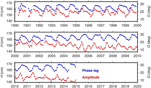
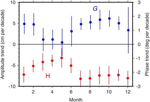
In light of the recent decadal trend, combined with a changing seasonal cycle, it will be useful in Section 3 to know whether the trend is occurring similarly for each month. This is confirmed by Fig. 5, for which linear trends were computed from the monthly estimates of M₂ over the 2000–2014 interval. All months throughout the year show the same decreasing amplitudes and increasing phase lags, although of smaller magnitudes for March through May (for which the phase changes are not statistically significant). Importantly, during the summer months — times when satellite altimetry is available — both amplitudes and phases show their greatest changes.

Fig. 5 Linear trends over the 2000–2014 interval in monthly estimates of the M₂ tide at Churchill, separated according to month of observation. Amplitude H (centimetres per decade) in red; phase lags G (degrees per decade) in blue. Error bars (1−σ) account for autocorrelation in the residuals of fit. Amplitude trends are negative for all months, and they are most significantly negative in those months for which satellite altimeter data are available offshore.

It must be acknowledged that a decline in amplitude accompanied by an increasing phase lag is a classic hallmark of a degraded tide-gauge response, of the sort that happens when an intake to a stilling well is increasingly obstructed. However, correspondence with the Canadian Hydrographic Service in June 2007 has led to no reported instrument problems. Ron Solvason, previously the Tidal Officer in that region, but now retired, noted (personal communication, June 2007) that the tide gauge had sat in a stilling well at the Churchill wharf until the early 1980s when its intake collapsed. The gauge was subsequently moved into a cell of an old pump house of the Port of Churchill, with an intake from the Churchill River consisting of a 30-inch diameter pipe, which rusted over time and also partially collapsed. An 18-inch pipe was inserted into the old pipe, with repairs completed around 2002. Since then there have been no reports of problems, aside from the anomalous tides reported here.

Wolf, Klemann, Wünsch, and Zhang (2006) give a useful overview of the earlier history of the Churchill tide gauge (see also Barnett, 1966; Tushingham, 1992).

The fact that there are no other permanent gauges in Hudson Bay, and in light of possibly important connections with climatic changes in sea ice, it seems advisable to attempt to examine the tide in the vicinity of Churchill remotely.

3 Satellite altimeter tide estimates

Although extraction of tidal signals from satellite altimeter measurements is nowadays a routine endeavour over the open ocean (Le Provost, 2001), it is more challenging in a location like Hudson Bay where seasonal ice cover exists for a large fraction of the year. Figure 6 shows the primary repeating ground tracks for the T/P-Jason series of satellites, colour-coded according to percentage of passes that return valid ocean heights. The highest return rates are only around 40%, and most locations return less. As Fig. 7 shows, most of the valid data are obtained from July to November.

Fig. 6 Ground track locations of the T/P and Jason series of satellites, colour coded to the percentage of Jason-1 passes returning valid ocean data. (Percentages are similar for T/P and Jason-2.) Crossovers A through E are locations where the tides have been estimated from the altimeter data of each separate mission (T/P, Jason-1, and Jason-2); see Table 2.

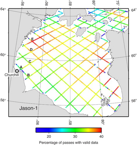
Fig. 7 Number of valid ocean altimeter returns obtained in each calendar month by the Jason-1 altimeter at the five crossover locations (A–E) shown in Fig. 6. These locations are mostly ice free only in the months July through October. No valid data at all are returned during January through April.

Because of the sparseness of altimeter data, the most accurate tidal estimates are likely to be those restricted to crossover locations where the number of valid data are approximately double that of typical along-track locations. The crossover location closest to the Churchill tide gauge, labelled “A” in Fig. 6, is of the greatest interest for comparison with the tide gauge. Unfortunately, this crossover location has relatively little valid ocean data, probably owing to its proximity to land, so an additional four crossover locations will be examined below; they are labelled “B” through “E” in the figure and run northwards along the western side of Hudson Bay. Because numerical models indicate that the M₂ tidal amplitudes exceed 1 m along the whole western coastline of the bay (e.g., St-Laurent et al., 2008), all crossovers A–E should detect robust M₂ amplitudes of that order.

The data underlying Figs 6 and 7 are based on Geophysical Data Records (GDRs) for ocean-tracked waveforms as released by the National Aeronautics and Space Administration (NASA) and the Centre National d’Études Spatiales (CNES) project teams, with some fields subsequently updated as described by Beckley et al. (2013). Owing to the environmental conditions in Hudson Bay, it is important to test for the presence of ice within the altimeter footprint, because ice echoes would tend to skew waveforms and to bias elevations too high. Most of the missions appear to set ice flags on a rather ad hoc basis, fine-tuned by experience. For TOPEX, an ice flag was set when the satellite was overflying locations where a climatological sea-ice dataset predicted a likelihood of ice and, in addition, the backscatter coefficient σ⁰ exceeded a certain threshold or the noise in 10 Hz wave-height estimates exceeded a threshold (Phil Callahan, personal communication, 2015). For Jason-1 the ice flag was set similarly although based only on σ⁰ and the ice climatology. For Jason-2 (still operating as of this writing) there are two ice flags, one based primarily on the altimeter measurement and the other based solely on the radiometer measurement. The first flag is set similarly to the Jason-1 criterion, plus it is set if the difference between two wet-tropospheric range corrections — one based on a meteorological model and the other based on the radiometer 23.8 GHz and 34.0 GHz brightness temperatures — exceeds a certain threshold. The second flag is set if the difference between the 34.0 GHz and 18.7 GHz brightness temperatures falls below a certain threshold (Dumont et al., 2011). The Jason-2 GDRs also contain two rain flags, one again based on a combination of the altimeter and radiometer data and one based solely on the radiometer data. The altimeter rain flag appears to be set too often, at least over Hudson Bay. In fact, at crossover location A the altimeter rain flag is set for every Jason-2 point, so any test on that flag would yield no data at all. (Note that version 3 of the Radar Altimeter Database System (Scharroo, 2012) combines the ice and rain flags for Jason-2, so users of those data should not test against that flag, or at least not at this location.)

The goal of this exercise is to investigate changes in the tide, so the altimeter time series must be partitioned in some fashion. It is not feasible to produce annual estimates of tides similar to those at the tide gauge, even at crossover locations. In light of the changes seen in Fig. 1, where the amplitude drops from about 153 cm in 2000 to about 146 cm in 2010, a precision of at least 2 cm is needed from the altimetry; 1 cm would be better. In addition, because of the inherent aliasing of tidal signals in altimetry, especially with more than half of each year being without data, the stability of the least-squares tidal inversions must be monitored. For example, at a single (non-crossover) location, the alias periods of P₁ and K₂ are 88.9 and 86.6 days, respectively (e.g., Schrama & Ray, 1994), requiring in principle nine years to decouple. In low latitudes, the use of crossover data would immediately break this coupling, because ascending and descending arcs tend to sample K₂ roughly in phase but P₁ out of phase. However, in high latitudes near the satellite turning latitude, this kind of favourable phase sampling no longer occurs and separation is more difficult. A response analysis can help because P₁ and K₂ can be tied to larger constituents, but there are other aliasing issues, some involving larger constituents.

Thus, as a preliminary exercise, the altimeter time series at crossover point E has been repeatedly analyzed with longer and longer segments of data in order to determine roughly how much altimetry is required to obtain sufficiently precise and stable estimates of M₂ to confirm, or not, the M₂ changes seen at Churchill. Two indicators of quality have been computed and are displayed in Fig. 8: (i) the standard error in M₂ and (ii) the largest correlation between any two estimated parameters (excluding Sa, which will always be problematic because data from more than half its period is always missing). Criterion (i) is the most important for the problem at hand, but (ii) is useful as a check on the robustness, or possible multicollinearity, of the linear system. The correlations were computed from the full least-squares error covariance matrix. Figure 8 suggests that standard errors less than 1.5 cm and overall correlations less than 0.5 can be obtained from 5-year segments. But recall that crossover point E yields more data than average, so somewhat more than 5-year segments are preferable. It seems the simplest approach is to compute tides from each separate satellite mission — T/P, Jason-1, and Jason-2 — which gives data segments of nine years, seven years, and seven years, respectively (with some minimal overlap).

Fig. 8 Quality of altimeter tide estimates at crossover location E as a function of length of the altimeter time series (where “years” actually means ice-free seasons). The solid line is the standard error (cm) of M₂ tidal estimates; the dashed line is the largest (absolute) correlation between estimated parameters, which is generally between constituents P₁ and K₂ (discounting Sa with itself).

The resulting altimeter-based estimates of the M₂ tide are listed in Table 2. The smallest standard errors, as anticipated from the sampling at each crossover location (Fig. 6), occur at location E, and the largest errors occur at location A. At all locations, even crossover A, the errors appear small enough to check for large trends in M₂. At three locations (A, B, and C) the estimated amplitudes agree among all three missions within their standard errors. The Jason-2 estimate at crossover D and the Jason-1 estimate at crossover E are slightly more anomalous, but they agree within twice their standard errors. Thus, the estimated amplitudes display no sign of a downward trend similar to that seen in the tide-gauge series.

Table 2. Estimates of M₂ from altimetry at crossover locations.

	Location	Mission^a	Amplitude (cm)	Phase lag (°)
A	59.0°N, 93.5°W	TOPEX	143.1±2.9	31.9±1.2
		Jason-1	141.8±1.9	30.3±0.8
		Jason-2	143.5±1.9	29.0±0.8
B	58.3°N, 92.1°W	TOPEX	118.5±1.4	63.6±0.7
		Jason-1	119.2±1.9	62.9±0.9
		Jason-2	119.3±1.7	63.0±0.8
C	59.5°N, 92.1°W	TOPEX	84.1±1.3	24.1±0.9
		Jason-1	84.9±1.2	25.2±0.9
		Jason-2	85.2±1.3	22.8±0.9
D	60.6°N, 92.1°W	TOPEX	81.2±1.1	346.6±0.8
		Jason-1	81.4±1.0	346.3±0.7
		Jason-2	79.6±1.1	346.7±0.8
E	61.6°N, 92.1°W	TOPEX	99.4±1.0	320.2±0.6
		Jason-1	102.0±1.2	319.8±0.7
		Jason-2	100.0±1.4	320.3±0.8

^aValid ocean data returned from each mission spanned the following time periods: Topex (July 1993–August 2002); Jason-1 (June 2002–November 2008); and Jason-2 (July 2008–November 2014).

The tide estimates of Table 2 represent the ocean tide because the data were pre-corrected for the Earth's solid tide, including radial crustal deformation of the load tide. The latter was based on a global model (GOT4.7, Ray (2013)) with amplitudes for crossovers A–E of 1.5, 1.2, 1.3, 1.6, and 1.8 cm, respectively. Even if these values are in error because of errors in the underlying ocean model (or errors in the Earth's elastic parameters), they would not affect trends.

4 Discussion

The negative trend in annual M₂ amplitudes seen in the tide gauge at Churchill after 2000 occurs also for the individual months July–November (Fig. 5), and during those same months satellite altimetry detected no comparable trends. The tidal changes must be localized to the vicinity of the tide gauge, possibly to the harbour which sits just inside the mouth of the Churchill River (see map in Barnett (1966)). Without comparable observations from an independent source, instrument malfunction cannot be ruled out. But some further analysis of the data in hand is useful.

The measurements of sea level at Churchill, as well as the interpretation of those measurements, have long proved to be difficult. Wolf et al. (2006) give a useful summary history of both. Annual estimates of relative sea levels showed a decline of approximately 4.4 mm y⁻¹ over the 1940–1975 period, but a much greater decline of approximately 10.4 mm y⁻¹ for 1975–2001, and 16.3 mm y⁻¹ for 1975–1990. Since the early 1990s the trend has returned to about −4.4 mm y⁻¹.

Much of the sea level trend is also reflected in the mean high water (MHW) and mean low water (MLW) levels — see Fig. 9. Both display a slow drop for several decades after 1940, then a more rapid decline. However, since roughly 1995 — the period corresponding to the decline in semi-diurnal tidal amplitudes — the MHW continues to decline, but MLW levels off.

Fig. 9 Annual mean high and low water (cm), shown after removal of the 18.6-year nodal cycle. Both MHW and MLW are decreasing over most of the time span, a reflection of the large glacial isostatic adjustment at Churchill. The decrease in the amplitude of the M₂ tide since the 1990s coincides with MLW levelling off. The time series of high and low water was computed from the hourly data by employing a modified cubic spline (Ellis & McLain, 1977) for the required interpolations.

Vertical land motion at Churchill is unusually large owing to glacial rebound after removal of the Laurentide ice sheet. Modern global positioning system measurements at Churchill indicate an uplift of more than 10 mm y⁻¹ (Mazzotti, Lambert, Henton, James, & Courtier, 2011; Wolf et al., 2006). This could result in corrupted tidal estimates with reduced amplitudes if the gauge “dries out” at low tide, and it could also distort MLW. However, there is no indication of that in the hourly tidal curves. The lowest water level in the entire Churchill time series occurred on 22 March 2011, and examination of those data (at 3-minute sampling, the highest available) shows no evidence of truncation or other obvious problems that could affect estimates of the tide or of MLW.

Tides in rivers can be affected by streamflow of the river (e.g., Godin, 1999; Jay & Flinchem, 1997). In the present case the effects of the Churchill River on the tide at the Churchill gauge are likely to be fairly benign because the river is wide and the gauge is not far upstream from the mouth (see maps in, for example, Barnett (1966), as well as the website of the Canadian Hydrographic Service). Moreover, there appears to be no obvious dependence on river discharge. Figure 10 shows the discharge since 1972 at a river station upstream of Churchill. The very large change during the 1970s was caused by a river diversion project (Tushingham, 1992), and yet that caused no noticeable change in M₂. Aside from occasional months of anomalously high discharge, the average is nowadays very low compared with the early 1970s and nothing unusual has occurred over the past decade when M₂ has been changing.

Fig. 10 Average monthly discharge rates (m³ s⁻¹) of the Churchill River at hydrological station Red Head Rapids (58°70′7′′N, 94°37′20′′W). The large drop during the mid-1970s was caused by a major river diversion project after which most of the Churchill River was ultimately diverted into the Nelson River (Tushingham, 1992).

Thus, no firm conclusion at this point is at hand, except that whatever tidal changes are happening at Churchill are not happening in the open waters of Hudson Bay. The importance of the tide gauge at Churchill cannot be overstated, not only because of its isolation but also because it sits on the prime spot for monitoring the mantle's response to the loss of the Laurentide ice (Han, Ma, Chen, Thomson, & Slangen, 2015; Wolf et al., 2006). The problem provides motivation to further enhance the utility of satellite altimetry in this region, possibly by extending the standard ocean waveform analyses to attempt to handle partial or complete ice echoes (e.g., Fricker & Padman, 2012; Kwok, 2008; Peacock & Laxon, 2004). An analysis of the tidal seasonal cycle with altimetry (cf. Fig. 4) would be most valuable.

Acknowledgements

It is a pleasure to thank Philip Woodworth, David Pugh, Remko Scharroo, and Brian Beckley for useful discussions. Brian Beckley also helped with altimeter data processing. Tide-gauge data were obtained from the Canadian Hydrographic Service, Department of Fisheries and Oceans Canada. The Churchill River discharge data were obtained from the Water Survey of Canada.

Disclosure statement

No potential conflict of interest was reported by the author.

Additional information

Funding

This work was supported by the National Aeronautics and Space Administration through the Ocean Surface Topography program.

References

- Amin, M. (1985). Temporal variations of tides on the west coast of Great Britain. Geophysical Journal of the Royal Astronomical Society, 82, 279–299. doi: 10.1111/j.1365-246X.1985.tb05138.x
- Barnett, D. M. (1966). A re-examination and re-interpretation of tide gauge data for Churchill, Manitoba. Canadian Journal of Earth Sciences, 3, 77–88. doi: 10.1139/e66-006
- Beckley, B., Ray, R., Holmes, S., Zelensky, N., Lemoine, F., Yang, X., … Hausman, J. (2013). Integrated multi-mission ocean altimeter data for climate research: TOPEX/Poseidon, Jason-1, and OSTM/Jason-2 user's handbook. Pasadena: California Institute of Technology.
- Cavalieri, D. J., & Parkinson, C. L. (2012). Arctic sea ice variability and trends, 1979–2010. The Cryosphere, 6, 881–889. doi: 10.5194/tc-6-881-2012
- Doodson, A. T., & Warburg, H. D. (1941). Admiralty manual of tides. London: HMSO.
- Dumont, J. P., Rosmoiduc, V., Picot, N., Bronner, E., Desai, S., Bonekamp, H., … Scharroo, R. (2011). OSTM/Jason-2 Products Handbook, CNES Report SALP-MU-M-OP-15815-CN, Toulouse: Centre national d’Études Spatiales.
- Ellis, T. M. R., & McLain, D. H. (1977). Algorithm 514: A new method of cubic curve fitting using local data. ACM Transactions on Mathematical Software, 3, 175–179. doi: 10.1145/355732.355738
- Fricker, H. A., & Padman, P. (2012). Thirty years of elevation change on Antarctic Peninsula ice shelves from multimission satellite radar altimetry. Journal of Geophysical Research, 117, C02026. doi: 10.1029/2011JC007126
- Godin, G. (1986). Modification by an ice cover of the tide in James Bay and Hudson Bay. Arctic, 39, 65–67. doi: 10.14430/arctic2048
- Godin, G. (1988). Tides. Ensenada Baja California. Mexico: CICESE.
- Godin, G. (1999). The propagation of tides up rivers with special considerations on the Upper Saint Lawrence River. Estuarine, Coastal and Shelf Science, 48, 307–324. doi: 10.1006/ecss.1998.0422
- Han, G., Ma, Z., Chen, N., Thomson, R., & Slangen, A. (2015). Changes in mean relative sea level around Canada in the twentieth and twenty-first centuries. Atmosphere-Ocean, 53, 452–463. doi:10.1080/07055900.2015.1057100
- IHO. (2006). Harmonic constants: Product specification, edition 1.0 (Tech. Rep.). Monaco: Organisation Hydrographique Internationale.
- Jay, D. A., & Flinchem, E. P. (1997). Interaction of fluctuating river flow with a barotropic tide: A demonstration of wavelet tidal analysis methods. Journal of Geophysical Research, 102, 5705–5720. doi: 10.1029/96JC00496
- Ku, L.-F., Greenberg, D. A., Garrett, C. J. R., & Dobson, F. W. (1985). Nodal modulation of the lunar semidiurnal tide in the Bay of Fundy and Gulf of Maine. Nature, 230, 69–71.
- Kwok, R. (2008). Satellite remote sensing of sea-ice thickness and kinematics: A review. Journal of Glaciology, 56, 1129–1140. doi: 10.3189/002214311796406167
- Le Provost, C. (2001). Ocean tides. In L.-L. Fu & A. Cazenave (Eds.), Satellite altimetry and earth sciences: A handbook of techniques and applications (pp. 267–303). San Diego: Academic Press.
- Mazzotti, S., Lambert, A., Henton, J., James, T. S., & Courtier, N. (2011). Absolute gravity calibration of GPS velocities and glacial isostatic adjustment in mid-continent North America. Geophysical Research Letters, 38(24). L24311. doi: 10.1029/2011GL049846
- Munk, W. H., & Cartwright, D. E. (1966). Tidal spectroscopy and prediction. Philosophical Transactions of the Royal Society A: Mathematical, Physical and Engineering Sciences, 259, 533–581. doi: 10.1098/rsta.1966.0024
- Munk, W. H., Zetler, B., & Groves, G. W. (1965). Tidal cusps. Geophysical Journal of the Royal Astronomical Society, 10, 211–219. doi: 10.1111/j.1365-246X.1965.tb03062.x
- Peacock, N. R., & Laxon, S. W. (2004). Sea surface height determination in the Arctic Ocean from ERS altimetry. Journal of Geophysical Research, 109, C07001. doi: 10.1029/2001JC001026
- Prinsenberg, S. J. (1988). Damping and phase advance of the tide in western Hudson Bay by the annual ice cover. Journal of Physical Oceanography, 18, 1744–1751. doi: 10.1175/1520-0485(1988)018<1744:DAPAOT>2.0.CO;2
- Ray, R. D. (2013). Precise comparisons of bottom-pressure and altimetric ocean tides. Journal of Geophysical Research, 118, 4570–4584.
- Scharroo, R. (2012). RADS version 3.1: User manual and format specification. Retrieved from http://rads.tudelft.nl/rads/radsmanual.pdf
- Schrama, E. J. O., & Ray, R. D. (1994). A preliminary tidal analysis of TOPEX/POSEIDON altimetry. Journal of Geophysical Research, 99, 24799–24808. doi: 10.1029/94JC01432
- St-Laurent, P., Saucier, F. J., & Dumais, J.-F. (2008). On the modification of tides in a seasonally ice-covered sea. Journal of Geophysical Research, 113, C11014. doi: 10.1029/2007JC004614
- Tushingham, A. M. (1992). Observations of postglacial uplift at Churchill, Manitoba. Canadian Journal of Earth Sciences, 29, 2418–2425. doi: 10.1139/e92-189
- Wolf, D., Klemann, V., Wünsch, J., & Zhang, F.-P. (2006). A reanalysis and reinterpretation of geodetic and geological evidence of glacial-isostatic adjustment in the Churchill region, Hudson Bay. Surveys in Geophysics, 27, 19–61. doi: 10.1007/s10712-005-0641-x