Sensitivity of Northwest North Atlantic Shelf Circulation to Surface and Boundary Forcing: A Regional Model Assessment

ABSTRACT

The northwest North Atlantic shelves, influenced by both North Atlantic subpolar and subtropical gyres, are among the most hydrographically variable regions in the North Atlantic Ocean and host biologically rich and productive fishing grounds. With the goal of simulating conditions in this complex and productive region, we implemented a nested regional ocean model that includes the Gulf of Maine, the Scotian Shelf, the Gulf of St. Lawrence, the Grand Banks, and the adjacent deep ocean. Configuring such a model requires choosing external data to supply surface forcing and initial and boundary conditions, as well as the consideration of nesting options. Although these selections can greatly affect model performance and results, they are rarely systematically investigated. Here we assessed the sensitivity of our regional model to a suite of atmospheric forcing datasets, to sets of initial and boundary conditions constructed from multiple global ocean models and a larger scale regional ocean model, and to two variants of the model grid — one extending farther off-shelf and resolving Flemish Cap topography. We conducted model simulations for a 6-year period (1999–2004) and assessed model performance relative to a regional climatological dataset of temperature and salinity, to observations collected from multiple monitoring stations and cruise transect lines, to satellite sea surface temperature (SST) data, to coastal sea level estimates, and to descriptions and estimates of regional currents from literature. Based on this model assessment, we determined the model configuration that best reproduces observations. We find that although all surface forcing datasets are capable of producing model SSTs close to observed, the different datasets result in significant differences in modelled sea surface salinity (SSS), with the European Centre for Medium-range Weather Forecasts’ (ECMWF) global atmospheric reanalysis (ERA-Interim) performing best. We also find that initial and boundary conditions based on global ocean models do not necessarily produce a realistic circulation, whereas using climatological initial and boundary conditions (constructed from long-term, monthly-mean output from a larger scale regional model) improves model performance. Through this model assessment, we determine the model configuration that best reproduces observations and gain generally applicable insight into the factors that are key to accurate model performance.

RÉSUMÉ

[Traduit par la rédaction] Les plateaux nord-ouest de l'Atlantique Nord, sur lesquels influent à la fois les tourbillons subpolaire et subtropical de l'Atlantique Nord, figurent parmi les régions de cet océan aux propriétés hydrographiques les plus variables. De plus, ils comportent des zones de grande richesse biologique et productrices de poissons. Dans le but de simuler les conditions dans cette région complexe et productive, nous avons mis au point un modèle océanique régional imbriqué qui couvre le golfe du Maine, le plateau néo-écossais, le golf du Saint-Laurent, les grands bancs et la mer profonde adjacente. La configuration d'un tel modèle requiert la sélection de données externes qui reproduisent le forçage en surface, et les conditions initiales et limites, et nécessite l’évaluation d'options d'imbrication. Bien que ces éléments puissent grandement influer sur le rendement du modèle et sur ses résultats, ils sont rarement évalués systématiquement. Nous examinons donc la sensibilité de notre modèle régional relativement à des données de forçages atmosphériques, à des conditions initiales et limites construites à partir de multiples modèles océaniques mondiaux et d'un modèle océanique régional à grande échelle, ainsi qu’à deux variantes de la grille du modèle, dont une qui s’étend au-delà du plateau et qui reproduit la topographie du bonnet Flamand. La simulation couvre une période de 6 ans (1999 à 2004). Nous avons évalué le rendement du modèle en le comparant à des données climatologiques régionales de température et de salinité, à des observations recueillies à de multiples stations de surveillance, à des données de transects relevées par bateau, à des températures marines en surface (SST) issues de satellites, à des estimations du niveau côtier de la mer, et à des descriptions et estimations de courants régionaux provenant d'autres documents. Sur la base de cette évaluation, nous avons déterminé la configuration du modèle qui reproduit le mieux les observations. Nous notons que toutes les séries de données de forçage en surface peuvent produire des SST modélisées comparables aux observations. En revanche, les diverses séries entraînent des différences considérables de salinité simulée à la surface de la mer, bien que les réanalyses mondiales atmosphériques (ERA) du Centre européen pour les prévisions météorologiques à moyen terme (ECMWF) aient montré un rendement supérieur. Nous constatons aussi que les conditions initiales et limites provenant de modèles océaniques mondiaux ne produisent pas nécessairement une circulation réaliste, tandis que l'utilisation de conditions initiales et limites climatologiques (construites à partir de longues séries de sorties mensuelles moyennes issues d'un modèle régional à grande échelle) améliore le rendement du modèle. Grâce à cette évaluation, nous déterminons la configuration du modèle qui reproduit le mieux les observations et nous acquérons des connaissances concrètes sur les facteurs qui régissent principalement la qualité de la modélisation.

KEYWORDS:

• Atlantic
• circulation
• dynamics
• modelling
• numerical

1 Introduction

The northwest North Atlantic is host to biologically rich and productive fishing grounds. This high biological productivity may be partly attributed to the large dynamic and geographic complexity characterizing the North Atlantic shelves, which are influenced by both the North Atlantic subpolar and subtropical gyres (Loder, Petrie, & Gawarkiewicz, 1998), contain a semi-enclosed sea (e.g., Gulf of St. Lawrence) and important coastal currents (e.g., the Labrador Current), and exhibit the largest observed sea surface temperature (SST) variability in the North Atlantic (Thompson, Loucks, & Trites, 1988).

Whether the shelf circulation in this complex region can be well represented by global ocean models with low spatial resolution is questionable. Several examples illustrate that regional models have succeeded in simulating circulation and hydrography in sub-regions of the northwest North Atlantic — for the eastern Scotian Shelf (Han & Loder, 2003), the Newfoundland Shelf (Han, 2000; Han et al., 2008), the Newfoundland and Labrador Shelves (Han, 2005), or the entire eastern Canadian shelf (Urrego-Blanco & Sheng, 2012). In order to simulate conditions in this productive and dynamically complex region, external data in the form of surface forcing and initial and boundary conditions are required, and different options for model nesting must be considered. The selection of forcing and boundary treatment holds the potential to greatly affect model performance and results, but often the different choices are not systematically investigated. One recent study investigated this downscaling problem for a regional model of the Middle Atlantic Bight by assessing model skill comparing three global models, four regional models, and a regional climatology with observations (Wilkin & Hunter, 2013). Those authors found that a regional climatology performed as well as or better than the considered ocean models. Guo et al. (2013) evaluated downscaling of model output for the Gulf of St. Lawrence region and found that removing biases in sea surface temperature (SST) resulted in improved surface temperature and wind estimates in their model. Clearly, nesting choices can have a large impact on model performance and should be evaluated for each region. An even larger spread in model results resulting from nesting choices for the northwest North Atlantic would be expected (relative to the Middle Atlantic Bight) because of its extreme variability and large dynamical complexity.

Here we describe the implementation of a nested regional ocean model for the northwest North Atlantic shelves, including the Gulf of Maine, the Scotian Shelf, the Gulf of St. Lawrence, the Grand Banks, and the adjacent deep ocean. We assessed the sensitivity of our regional model to a suite of atmospheric forcing datasets, to sets of initial and boundary conditions constructed from different global ocean models and a larger scale regional ocean model, and to two variants of the model grid — one extending farther off-shelf and resolving Flemish Cap topography. We additionally evaluate the effect of including nudging of temperature and salinity to the observed regional climatology of Geshelin, Sheng, and Greatbatch (1999). The goals of this model assessment are twofold: (i) to determine the model configuration that best reproduces observations, and (ii) to gain generally applicable insight into which factors are key to accurate model performance.

2 Model description

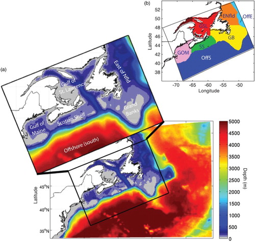
Our model, which we refer to as the Atlantic Canada Model (ACM), is based on the Regional Ocean Modelling System (ROMS), version 3.5, a terrain-following, free-surface, primitive equation ocean model (Haidvogel et al., 2008). The model domain includes the area between Cape Cod and the southern coast of Labrador (Fig. 1a), encompassing the Gulf of Maine, Scotian Shelf, Gulf of St. Lawrence, Grand Banks, east Newfoundland Shelf, and the deep-water region offshore to the south and east. The model's 240-by-120 horizontal grid (∼10 km horizontal resolution) is superimposed on the region from 36.1°N to 53.9°N and 74.7°W to 45.1°W. The ACM is also tested on an expanded model domain (34.4°N to 55.5°N and 74.7°W to 37.9°W, with a 300-by-150 horizontal grid at a similar ∼10 km resolution), which extends farther to the east and south and additionally includes Flemish Cap. The model (for both grid versions) has 30 vertical levels and its minimum water depth is 10 m. The model employs the generic turbulence length-scale (GLS gen) vertical mixing scheme (Umlauf & Burchard, 2003; Warner, Sherwood, Arango, & Signell, 2005) and a combination of nudging and radiation open boundary conditions (Marchesiello, McWilliams, & Shchepetkin, 2001). In its current set-up, the model output is produced as five-day time averages, which we note removes the variability associated with synoptic weather.

Fig. 1 (a) Northwest North Atlantic bathymetry (m) and Atlantic Canada Model (ACM) domain (outlined and in inset). (b) The model domain is divided into sub-areas for analysis: East of Newfoundland (ENfld), Grand Banks (GB), Gulf of St. Lawrence (GSL), Scotian Shelf (SS), Gulf of Maine (GOM), Offshore-south (OffS) and Offshore-east (OffE).

Surface forcing, initial conditions, and boundary conditions are provided from various external datasets (described in Section 2.a and Table 1). The ROMS interpolates surface forcing data from any regular grid and time step to the model grid and time, and preliminary processing is limited to converting surface forcing variables (e.g., shortwave radiation flux, longwave radiation flux, surface air temperature, pressure, humidity, precipitation, and winds) to the model units. Surface net heat flux and wind stress are internally calculated by ROMS’ ocean–atmosphere boundary layer model (Fairall, Bradley, Rogers, Edson, & Young, 1996; Fairall et al., 1996; Liu, Katsaros, & Businger, 1979). Initial and boundary conditions are produced by interpolating ocean data onto the model grid. Initial conditions are constructed by selecting the data on or nearest 1 January 1999, while boundary conditions are derived from the ocean data corresponding to the model domain edges (for all time steps). At open boundaries, a 10-grid-cell wide buffer zone is implemented in which the model's temperature, salinity, and velocity fields are nudged toward the parent model interpolated onto the model grid, with nudging strength decaying linearly away from the boundary to zero. Open boundary nudging strength is larger (by a factor of 20) for inflow than for outflow conditions, such that inflow is strongly specified by the open boundary (i.e., active condition), while outflow is more highly dependent on flow conditions within the model domain (i.e., passive condition) (Marchesiello et al., 2001). Climatological river runoff is included for 12 major rivers, including the St. Lawrence River and St. John River, based on the observed long-term monthly mean river discharge (using data available from Water Survey of Canada (Government of Canada, 2015)).

Table 1. Summary of external datasets providing atmospheric surface forcing data (CORE, NARR, ECMWF, ECMWF-EVAP) or ocean nesting data (HYCOM, MERCATOR, UBS).

Data ID	Details	Description
CORE	CORE, version 1 (Large & Yeager, 2004)	Informed by reanalysis and satellite data with interannually varying forcing and 2x2 horizontal resolution. Created by the Clivar Working Group for Ocean Model Development (WGOMD) for use in the Common Ocean-Ice Reference Experiments (CORE) for the period 1999–2004.
NARR	National Centers for Environmental Prediction (NCEP) North American Regional Reanalysis (NARR) (Mesinger et al., 2006)	Assimilates observed precipitation for improved hydrological cycling, with 29 vertical levels. Temporal resolution is 3 hourly, except daily net surface solar radiation, and temporal coverage extends from 1979 to 2012. Provided on Lambert Conformal Conic ∼32 km (0.3°) grid. We interpolated the data onto a ∼0.25° regular grid.
ECMWF	European Centre for Medium-range Weather Forecasts (ECMWF) global atmospheric reanalysis (ERA-Interim) (Dee et al., 2011)	Temporal resolution is 3 hours, except (daily) mean net surface solar radiation. Data are instantaneous values or time averages, with temporal coverage from 1979 through 2012, and spatial resolution includes 60 vertical levels, and T255 spectral grid (∼0.7°). We interpolated the data onto an ∼0.125° regular grid.
ECMWF-EVAP	Same as above	Same as above, but with evaporation additionally specified from the data (as opposed to being calculated internally within the model).
HYCOM	HYCOM+NCODA global 1/12° analysis, experiments 60.6–90.6	HYCOM 2.2 ocean model assimilates satellite observations of sea surface height (SSH) and SST, in situ expendable bathythermograph, ARGO float, and moored buoy T and S data via Navy Coupled Ocean Data Assimilation (NCODA; Cummings, 2005). Has 32 vertical levels, and uses the Navy Operational Global Atmospheric Prediction System (NOGAPS) surface forcing. Data assimilation is performed south of 47°N before 9/2008. We employ daily average output.
MERCATOR	MERCATOR GLORYS2V1	Employs Nucleus for European Modelling of the Ocean (NEMO) ocean model with 1/4° grid and 75 vertical levels (Barnier et al., 2006; Barnier & Ferry, 2011). Incorporates observations of satellite-derived SST and SSH, and in situ T and S, using reduced order Kalman filter (SEEK algorithm, see Pham, Verron, & Roubaud, 1998; Tranchant et al., 2008). Surface forcing from ECMWF ERA-Interim. We employ daily average output.
UBS	Urrego-Blanco and Sheng (2012) regional physical ocean model of the northwest North Atlantic	Based on NEMO physical ocean model, covers 33°N to 55°N in latitude, and 80°W to 33°W in longitude, with 1/4° horizontal resolution, 46 vertical levels, and a coupled sea-ice model. Using Geshelin et al. (1999) climatology as initial conditions and CORE surface forcing, the model was integrated (from an initial state of rest) in 1987 to 2004. We employ 5-day average model data from the last 6 years (1999–2004).
HYCOMdebias	Same as HYCOM	Replaced monthly mean T and S in each grid cell with that from the Geshelin et al. (1999) climatology.
MERCATORdebias	Same as MERCATOR	Replaced monthly mean T and S in each grid cell with that from the Geshelin et al. (1999) climatology.
UBSclim	Same as UBS	Long-term (1999–2004) monthly mean output from UBS.

a Description of External Datasets

We considered the following three atmospheric surface forcing datasets: the interannually varying Coordinated Ocean-Ice Reference Experiment (CORE) forcing (Large & Yeager, 2004), the National Centers for Environmental Prediction (NCEP) North American Regional Reanalysis (NARR) (Mesinger et al., 2006), and the European Centre for Medium-range Weather Forecasts' (ECMWF) global atmospheric reanalysis (ERA-Interim) (Dee et al., 2011; Table 1). Each dataset includes time-varying fields of air temperature, air pressure, humidity, surface winds, rain, shortwave radiation, and net downward longwave radiation. We additionally utilized evaporation data from ECMWF (instead of allowing ROMS to calculate evaporation), which we refer to as ECMWF-EVAP.

We sourced ocean-nesting information from two global ocean models and one larger regional ocean model: the Mercator Global Ocean Reanalysis and Simulations (GLORYS) (hereafter MERCATOR), the Hybrid-Coordinate Ocean Model (HYCOM) Navy Coupled Ocean Data Assimilation (NCODA) ocean model (hereafter HYCOM), and the larger regional ocean model of Urrego-Blanco and Sheng (2012; UBS). We created three additional datasets by modifying the original datasets. In the case of HYCOM and MERCATOR, we removed the monthly mean bias from each model grid cell for (three-dimensional) temperature and salinity relative to climatology (Geshelin et al., 1999) to produce debiased datasets: HYCOMdebias and MERCATORdebias. For UBSclim, a climatological version of the UBS regional model output without interannual variability, we calculated the long-term monthly mean UBS output. Table 1 summarizes the external datasets.

3 Methodological approach

There are a number of choices when setting up a regional ocean circulation model. Ideally, the effect of every choice on model performance would be tested. In reality, it is not practical to perform the high number of simulations and analyses that would be required. To constrain the problem, we defined four axes of variability to investigate: first, the effect of selecting different surface forcing data; second, the effect of ocean model nesting selection (i.e., varying the ocean model from which we derive initial and boundary conditions); third, the effect of nudging the model's temperature and salinity to climatology (i.e., an application of no, weak, or moderate nudging); and fourth, the impact of modifying the model grid — in this case, expanding the domain to the east and south, thereby including Flemish Cap and the slope of the Newfoundland and Labrador Shelves, which are potentially important for accurate representation of the Labrador Current.

We performed a number of model simulations for each set of model choices. In each simulation, the initial conditions vary with the boundary conditions (i.e., the initial conditions are derived from the same dataset as the boundary conditions). The simulations were conducted over the 6-year period 1999–2004. Runs performed using initial and boundary information from the global HYCOM model are an exception because HYCOM output is only available beginning in November 2003. The HYCOM-based runs span the years 2003 to 2008. Although the later HYCOM time period could result in different ocean states as a result of interannual variability, because we evaluate the model simulation with respect to observations from 2003 to 2008, we expect any bias in the model assessment to be minimized. A long simulation with UBSclim initial and boundary information was also performed over the period 1999–2008 (in order to compare with all other simulations). The model simulations are listed in Table 2.

Table 2. Atlantic Canada model (ACM) simulations.

Run ID	Surface Forcing	Nesting	Interior Nudging	Grid
Vary Surface Forcing
ACM-CORE	CORE	UBSclim	N/A	Orig
ACM-NARR	NARR	UBSclim	N/A	Orig
ACM-ECMWF	ECMWF	UBSclim	N/A	Orig
ACM-ECMWF-EVAP	ECMWF+EVAP	UBSclim	N/A	Orig
Vary Nesting Data
ACM-UBS	ECMWF	UBS	N/A	Orig
ACM-UBSclim	ECMWF	UBSclim	N/A	Orig
ACM-HYCOM	ECMWF	HYCOM	N/A	Orig
ACM-MERCATOR	ECMWF	MERCATOR	N/A	Orig
ACM-HYCOMdebias	ECMWF	HYCOM debiased	N/A	Orig
ACM-MERCATORdebias	ECMWF	MERCATOR debiased	N/A	Orig
Vary Nudging
ACM-UBSclim	ECMWF	UBSclim	N/A	Orig
ACM-buff-UBSclimTS	ECMWF	UBSclim	N/A	Orig
ACM-buff-GeshTS	ECMWF	UBSclim	N/A	Orig
ACM-buff-GeshTS -interior120day	ECMWF	UBSclim	120 day (weak)	Orig
ACM-buff-GeshTS -interior60day	ECMWF	UBSclim	60 day (moderate)	Orig
Vary Model Grid
ACM-Original	ECMWF	UBSclim	N/A	Orig
ACM-Large	ECMWF	UBSclim	N/A	Large

Note: ACM-UBSclim, ACM-Orig, and ACM-ECMWF are the same simulation.

We assessed model performance by comparing model output with both observations and the climatological monthly temperature and salinity dataset by Geshelin et al. (1999). Observations are from the Atlantic Zone Monitoring Program (AZMP; Fisheries and Oceans Canada, 2011) and include conductivity-temperature-depth (CTD) measurements from fixed monitoring stations and repeat cruise transects located on the Scotian Shelf, Gulf of St. Lawrence, Grand Banks, and the Newfoundland and Labrador Shelves (Therriault et al., 1998). We compared the AZMP data directly with model temperature and salinity. For cruise transects, model output was sampled along each AZMP section at the corresponding time; for monitoring stations, model output was sampled from the entire water column at the model grid cell nearest each station, and the AZMP observations were depth binned and averaged within each bin to correspond to the model depths.

We also utilized satellite-derived SSTs. We used the Advanced Very High Resolution Radiometer (AVHRR) Pathfinder Level 3 Daily Daytime SST, Version 5, data product on a grid of approximately 0.044° (4 km resolution at the equator) for the years 1999–2006 (Kilpatrick, Podesta, & Evans, 2001; ftp://podaac-ftp.jpl.nasa.gov/allData/avhrr/L3/pathfinder_v5/daily/day). We also used the National Aeronautics and Space Administration (NASA), Jet Propulsion Laboratory (JPL), Group for High Resolution Sea Surface Temperature (GHRSST) Level 4 Operational Sea Surface Temperature and Sea Ice Analysis (OSTIA) Global Foundation SST Analysis Product (hereafter GHRSST) on a 0.054° grid (ftp://podaac-ftp.jpl.nasa.gov/allData/ghrsst/data/L4/GLOB/UKMO/OSTIA/) for the years 2007–2008. We note that there is an offset between summer SST values determined using SST values from AVHRR and those from climatology (Geshelin et al., 1999): mainly, the AVHRR SSTs are warmer than climatology in summer. The origin of this seasonal bias is unknown. Although it may appear sufficient to compare model SST results solely with the climatological values of Geshelin et al. (1999), the climatology is not necessarily independent of the model results. For example, the model is nudged to the climatology in runs ACM-buff-GeshTS (nudging occurs only in the boundaries and buffer zone), ACM-buff-GeshTS-interior120day, and ACM-buff-GeshTS-interior60day (nudging occurs at all model grid cells). Also, model runs employing UBS model data (e.g., as initial and boundary conditions) are indirectly influenced by the climatology because the UBS model is initialized from this climatology and employs a spectral nudging method to the climatological dataset. The AVHRR SST dataset thus adds an independent point of comparison.

We compared time series of model temperature and salinity, at the sea surface and bottom, averaged over the entire model domain and for domain sub-areas (see Fig. 1b), with the regional climatological temperature and salinity (Geshelin et al., 1999). In order to compare model output directly with the climatology, we interpolated the monthly climatological data to the model time and the model grid. For SST, we also compared the simulated SST time series with satellite SSTs. In order to facilitate the comparison, we regridded high quality, daily AVHRR (GHRSST) SSTs onto the model grid (quality flag ≥4 and error flag ≤4°C for AVHRR and GHRSST, respectively). We discarded interpolated values located more than 1/8° from the satellite observations. We calculated five-day averages of the interpolated satellite SST (to compare directly with the model's five-day time averages). Simulated and climatological SSTs were extracted only from grid cells where satellite data exist, then the domain-wide and sub-domain area averages were calculated (time series of salinity use all grid locations in the areal average). We determined statistical metrics of bias, accuracy (root-mean-square error (RMSE)), and correlation (Pearson's R²) between the simulated and observed values.

Finally, we evaluated sea level and currents in the model with respect to observations. We supplemented that quantitative assessment with qualitative evaluation of simulated surface velocity fields using descriptions of key dynamical features in the region from the literature. In order to compare sea level in the model with observations, total sea level at multiple coastal monitoring stations (Halifax, Yarmouth, Rimouski, Saint-Francois, Sept-Îles, and Charlottetown) was extracted from the Fisheries and Oceans Canada tide gauge dataset (Fisheries and Oceans Canada, 2015; http://extrememarine.ocean.dal.ca/dalcoast/Canada.php) for the time period 1999–2001. Because the model does not include tides, the tidal component of sea level at each station was estimated using a harmonic analysis of ocean tides (Pawlowicz, 2011; Pawlowicz, Beardsley, & Lentz, 2002). The tidal component was then removed from the total sea level (via differencing) to determine the non-tidal sea level at each monitoring station, which is directly comparable to model sea level. We then compared the non-tidal sea level time series (1999–2001) at each monitoring station with the closest model ocean grid point and computed statistical measures of the time series’ performance for each model simulation.

As an alternative approach to assessing regional circulation in the model, volume transports were determined at multiple locations, including sections representing the Labrador Current and the Nova Scotia Current (NSC). Simulated long-term mean volume transports were compared with observation-based estimates of annual mean transports from Loder et al. (1998). Modelled volume transports were calculated utilizing the criterion of S < 34.8 following Loder et al. (1998). Section locations were chosen in the model to correspond as closely as possible to the sections listed by Loder et al. (1998) in their Table 1 and Fig. 5.2. These sections include the Labrador Current at Hamilton Bank off the southern coast of Labrador (7.5 Sv (1 Sv=10⁶m³s⁻¹) from Lazier and Wright (1993)), the Labrador Current transport through Flemish Pass (5.8 Sv from Petrie and Buckley (1996)) and around the Tail of the Grand Banks (3.2 Sv from Petrie and Drinkwater (1993)), and the NSC at the Halifax Section (0.70 Sv from Anderson and Smith (1989)). Because the Hamilton Bank section from Loder et al. (1998) is situated slightly north of the model domain's northern edge, we compare that volume transport with section LC1 located within our model domain and south of the model buffer zone.

In the following sections, we investigate the effects on model performance of varying surface forcing and model nesting data, of nudging the model toward climatology, and of expanding the model grid.

4 Model assessment I: Effect of surface forcing selection

We performed four simulations differing only by the surface forcing dataset selected (Table 2). All simulations used UBSclim ocean initial and boundary conditions. We refer to these simulations as ACM-CORE, ACM-NARR, ACM-ECMWF, and ACM-ECMWF-EVAP. Below we assess these model simulations.

Time series of area-averaged sea surface properties (temperature and salinity) are constructed for the entire model domain and the sub-areas shown in Fig. 1b. Salinity is compared with climatological values (Geshelin et al., 1999), and temperature is compared with both climatology and an AVHRR satellite SST dataset. Figure 2 presents the time series of ACM-NARR, ACM-ECMWF, and ACM-CORE with those generated from climatology and the AVHRR data.

Fig. 2 Time series of SST and SSS, averaged over (a) the entire ACM domain and (b) sub-areas from simulations with varied surface forcing (ACM-ECMWF, ACM-NARR, and ACM-CORE), with time series of climatology (grey dashed line) and satellite SST (grey stars) for comparison.

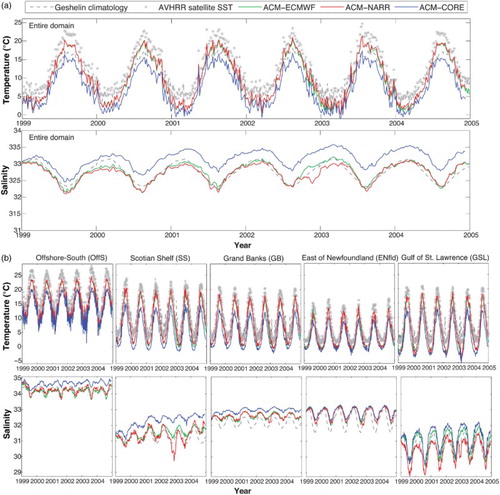
The surface time series averaged over the entire domain (Fig. 2a) and regions of the model domain (Fig. 2b) reveal that the model performs reasonably well using either NARR or ECMWF surface forcing. The statistical results are presented in Table S1a (supplementary data). The domain-averaged SST is well correlated with the Geshelin climatology (AVHRR), with R² values of 0.97 and 0.96 (0.99 and 1.00) for ACM-NARR and ACM-ECMWF, respectively. Seasonality is generally well captured although the simulated winter SST is cooler than climatology and AVHRR. In summer, modelled SST lies between the climatological and satellite values (i.e., warmer than climatology but cooler than satellite SST). Sea surface salinity (SSS) is also simulated well, with domain-wide R² values of 0.80 and 0.85 for ACM-NARR and ACM-ECMWF, respectively. Differences in SSS are mainly located in the Gulf of St. Lawrence, where ACM-NARR is fresher, and on the Scotian Shelf, where ACM-NARR is fresher from 2002 to mid-2003. We conclude that both ECMWF and NARR surface forcing result in good distributions of surface temperature and salinity in the model.

In contrast, the ACM-CORE time series is consistently cooler than climatology and observations in both summer and winter. ACM-CORE exhibits higher SSS than ACM-NARR and ACM-ECMWF and the climatology (see Fig 2a and 2b). ACM-CORE is also outperformed in the statistical assessments of simulated bottom temperature and salinity time series by ACM-NARR and ACM-ECMWF, which are quite similar to one another (see Table S1a). The CORE surface forcing dataset clearly produced poorer model results, likely because of CORE's low horizontal resolution (2° compared with 0.3° and 0.7° for NARR and ECMWF, respectively) and low temporal variability for precipitation (monthly) (Griffies, Winton, & Samuels, 2004). When analyzing surface heat and moisture fluxes (e.g., surface net heat flux, surface net moisture flux, net solar shortwave radiation flux, net longwave radiation flux, net latent heat flux, and net sensible heat flux) in the model simulations, we found that ACM-CORE exhibits a more positive surface net salt flux (i.e., net evaporation, for the flux defined as salinity x (E-P), where E is evaporation, and P is precipitation) in all regions, while ACM-NARR and ACM-ECMWF have very similar surface net moisture fluxes. ACM-NARR and ACM-ECMWF also produce similar surface net heat fluxes, while ACM-CORE fluxes are slightly offset to more negative values (i.e., net heat loss, corresponding to ocean cooling), especially in the offshore region.

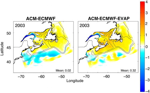
The final surface forcing dataset, ECMWF-EVAP, allows us to evaluate whether model performance can be improved by specifying the reanalysis evaporative surface flux in the model, as opposed to allowing ROMS to calculate evaporation as a function of air temperature and humidity. In the simulation employing evaporation data, ACM-ECMWF-EVAP, surface and bottom temperature are essentially unchanged, while SSS increases in the Offshore-South area, over the shelves including the Scotian Shelf and Grand Banks, and in the Gulf of St. Lawrence, increasing the positive salinity bias over those regions (Fig. 3). The 2003 mean annual SSS anomaly relative to climatology is mapped in Fig. 3. The northeastern quadrant of the domain (Offshore-East and eastern Newfoundland Shelf) is unaffected. The R² value for the average SSS time series in the domain is reduced (to 0.80 from 0.85 in ACM-ECMWF), and the RMSE is slightly increased (see Table S1a). Based on the statistical comparison of model results with observations and climatology, we conclude that specifying evaporation does not improve model performance.

Fig. 3 Mean annual SSS anomaly (model-climatology) in 2003.

There are several model biases (relative to the climatology) in the shelf regions that are common across simulations with varied surface forcing (Fig. 2b, Table S1a). First, model SSS is higher in the eastern Newfoundland Shelf and eastern Gulf of St. Lawrence regions (small bias) and fresher in the lower St. Lawrence Estuary than observations. Bottom salinity is consistently too high in the western Scotian Shelf and too fresh on the eastern Scotian Shelf, such that the model's east–west bottom salinity gradient on the Scotian Shelf is weaker than that indicated by the climatology. In terms of bottom temperatures, the Grand Banks is too warm, and the eastern Scotian Shelf and Gulf of Maine are too cool. Next we assess how different ocean-nesting treatments, the application of nudging, and changes in model grid affect the ACM-NARR and ACM-ECMWF results.

5 Model assessment II: Effect of ocean model nesting

The effect of model nesting is investigated by varying the physical initial and boundary information (temperature, salinity, velocities, and sea surface height) provided to the ACM. We performed six simulations differing only in which ocean model nesting dataset was selected (all utilize ECMWF surface forcing). We refer to these simulations as ACM-HYCOM, ACM-MERCATOR, ACM-UBS, ACM-HYCOMdebias, ACM-MERCATORdebias, and ACM-UBSclim (Table 2). All simulations are for the time period 1999–2004, except the HYCOM simulations because HYCOM data are only available starting in November 2003. We therefore performed simulations with HYCOM data from 2003 to 2008 and conducted one extended simulation (1999–2008) using regional model output (ACM-UBSclim-long) for comparison purposes.

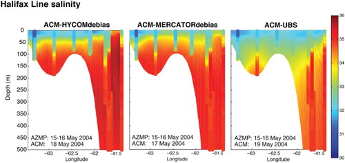
Nesting the ACM in either of the global ocean models, HYCOM or MERCATOR, results in poor model performance, irrespective of whether we utilize the original or debiased initial and boundary datasets. We assessed model salinity and temperature along the AZMP cruise transects located in the model domain. Figure 4 depicts the vertical salinity distribution along the Halifax Line transect in May 2004 in the model and from AZMP observations. The ACM-HYCOMdebias and ACM-MERCATORdebias simulations produce a poorly simulated shelf vertical structure: salinity is too high on the shelf (this is the case when using either debiased or non-debiased ocean-nesting datasets). The SSS biases and RMSEs are significantly higher in those simulations employing initial and boundary conditions derived from HYCOM and MERCATOR (Table S1b).

Fig. 4 Model salinity along the Halifax Line transect, overlain by AZMP observations, in May 2004, for three simulations: ACM-HYCOMdebias, ACM-MERCATORdebias, and ACM-UBS.

Although SSS is not well simulated when using HYCOM or MERCATOR boundary information, simulated SSTs are realistic. Averaged over the model domain, ACM-MERCATOR exhibits the smallest RMSE and bias relative to satellite observations and the climatological SST of all 6-year long simulations (Table S1b). ACM-HYCOM SST also performs well. When we compare ACM-HYCOM and ACM-HYCOMdebias directly with ACM-UBSclim-long for the same time period (2004–2008), ACM-HYCOM exhibits the smallest RMSE of the three simulations in domain-averaged SST for both satellite and climatology (RMSE = 1.56°C and 1.18°C, respectively). However, neither bottom temperature nor bottom salinity is well represented by the model when initial and boundary conditions are provided by HYCOM, MERCATOR, or their debiased versions (Table S1b).

In contrast to the simulations using initial and boundary information sourced from global ocean models, ACM-UBS and ACM-UBSclim both simulate shelf conditions adequately. In ACM-UBS the vertical structure of salinity on the Halifax Line is similar to AZMP observations (Fig. 4 shows the comparison in May 2004) although the deepest shelf water (∼150–175 m) is not as saline as observations. The ACM-UBS and ACM-UBSclim simulations produce very similar time series of temperature and salinity at the surface and bottom averaged over all the sub-areas (not shown). Only small differences in SSS and bottom temperature and salinity are found between the ACM-UBS and ACM-UBSclim simulations. In the offshore regions the ACM-UBS simulation is slightly saltier in winter and spring than the ACM-UBSclim simulation. On the Scotian Shelf, ACM-UBSclim exhibits slightly cooler and fresher bottom waters relative to climatology (and the bottom waters on the Scotian Shelf in the ACM-UBSclim are also fresher than in the ACM-UBS simulation).

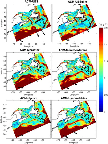
Both ACM-UBS and ACM-UBSclim perform well with respect to climatology. Comparisons of the time series of domain-averaged SSS and SST to climatology show very similar statistical results. The ACM-UBSclim R² values are incrementally higher for SSS (by 0.06) and identical for SST (see Table S1b). In the comparison with satellite SST, domain-averaged R² values are identical (1.00), whereas the ACM-UBSclim domain-averaged bias and RMSE increase slightly (by 0.15°C). ACM-UBSclim exhibits small improvements in statistical metrics for bottom salinity and temperature (higher R² values by 0.01 and 0.23, and lower RMSE by 0.03° and 0.06°C, respectively). However, small differences in the statistical measures are likely not meaningful. Surface velocity fields (shown for year 2004 in Fig. 5) indicate that for ACM-MERCATOR, ACM-HYCOM, ACM-MERCATORdebias, and ACM-HYCOMdebias the Gulf Stream may be situated too close to the shelf slope and that the annual mean shelf break current transport can occur toward the northeast, which is in the opposite direction from observed. The Gulf Stream in the southern portion of the domain is displaced further from the shelf break in ACM-UBSclim, and the shelf break current is stronger (Fig. 5). We conclude that of the varied ocean-nesting set-ups, ACM-UBS and ACM-UBSclim perform best. We prefer to use the monthly climatological boundary conditions, UBSclim, over the 5-day varying UBS because simulations using UBSclim are not confined to the specific time period of the parent model.

Fig. 5 Annual mean surface velocity (m s⁻¹) mapped in 2004 for each simulation with varying ocean nesting (ACM-UBS, ACM-UBSclim, ACM-MERCATOR, ACM-MERCATORdebias, ACM-HYCOM, and ACM-HYCOMdebias). Vector arrows (black) are drawn at identical locations for comparison.

We compared the simulations using debiased MERCATOR and HYCOM datasets, ACM-MERCATORdebias and ACM-HYCOMdebias (which are debiased with respect to the Geshelin climatology), with the complete set of observational data, including AZMP measurements, satellite SST, and the Geshelin climatology. Here we note that the comparison with Geshelin climatology is not independent. Despite this, debiasing does not improve the simulations’ bias relative to climatology, as shown below.

Debiasing the MERCATOR and HYCOM datasets produced mixed results. In the case of MERCATOR, debiasing had no discernable effect on modelled SST, but improved bottom temperature in most sub-regions (except the Gulf of St. Lawrence and the Scotian Shelf). The SSS improved greatly in the easterly portion of the domain (Offshore-East, the Grand Banks, and the eastern Newfoundland Shelf), but only slightly on the Scotian Shelf. Debiasing created negligible improvement in the lower St. Lawrence Estuary, the Gulf of St. Lawrence, and the Scotian Shelf where non-trivial bottom salinity biases exist. Some improvement in bottom salinity was apparent in the Grand Banks and the eastern Newfoundland Shelf. Similar changes were identified in ACM-HYCOMdebias, though bottom salinity in the Grand Banks and eastern Newfoundland Shelf did not improve (as occurred in ACM-MERCATORdebias). The SSS was again improved in the eastern portion of the domain in ACM-HYCOMdebias. The net improvement in bottom temperature in ACM-HYCOMdebias likewise occurred in most regions (except in the Scotian Shelf, Grand Banks, and eastern Newfoundland Shelf).

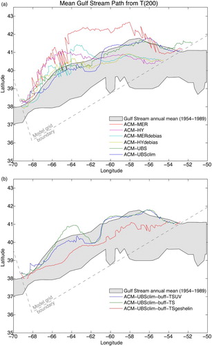
We also explored the position of the Gulf Stream in the model simulations with varied ocean nesting. We utilized the Gulf Stream North Wall (GSNW) index, following Joyce, Deser, and Spall (2000), who defined this metric to be the location of the 15°C isotherm at 200 m depth. Figure 6 compares the long-term mean GSNW position in each model simulation with the range of annual mean positions determined from observations over a 36-year period (1954–1989) by Joyce et al. (2000). In most simulations, the Gulf Stream is situated too far north and too close to the shelf, relative to the observed location (Fig. 6a). In the ACM simulations that use raw initial and boundary information from global ocean parent models, the Gulf Stream assumes the most northerly positions: ACM-MERCATOR (red) and ACM-HYCOM (pink). In the ACM simulations with debiased MERCATOR and HYCOM boundary information the GSNW position is too far northeast of approximately 62°W: ACM-MERCATORdebias (turquoise) and ACM-HYCOMdebias (gold). Finally, the Gulf Stream is positioned mainly within the range of observed values in the ACM-UBS (green) and ACM-UBSclim (blue) simulations.

Fig. 6 The observed range of mean annual GSNW index locations (black outline with grey shading) (see Fig. 5 in Joyce et al., 2000) with the long-term mean position of the ACM simulations (coloured lines) with (a) varied ocean nesting and (b) varied treatment of buffer zone nudging. The grey dashed line indicates the model grid boundary.

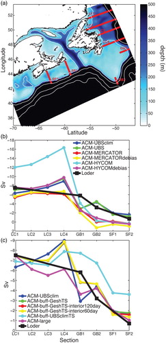
Finally, we assessed the simulations with respect to observed currents and coastal sea level. We compared the annual mean transports listed by Loder et al. (1998) for the Labrador Current (at Hamilton Bank, Flemish Pass, and Tail of the Grand Banks) and the NSC and shelf break current (at the Halifax Line) with the simulated long-term mean transport at sections LC1, GB1, GB2, and SF2. Section locations are mapped in Fig. 7a. The model transports are most similar to the estimated transports of Loder et al. (1998) when we apply the UBS and UBSclim initial and boundary conditions (RMSE = 1.6 Sv and 1.7 Sv, respectively), as shown in Fig. 7b. Debiasing HYCOM improves model transport at LC1 and GB2, but debiasing MERCATOR produces no such improvement (and transport worsens at the GB1 and GB2 section; Fig. 7b). Using HYCOM or MERCATOR boundary conditions, RMSE values range from 2.1 Sv (for ACM-HYCOMdebias) to 3.2 Sv (for ACM-MERCATORdebias).

Fig. 7 (a) Section locations for model long-term mean volume transport comparison to the estimated mean annual transport listed by Loder et al. (1998). LC1, GB1, GB2, and SF2 correspond to their Hamilton Bank, Flemish Pass, Tail of the Grand Banks, and Halifax Section, respectively (see their Table 1 and Fig. 5.2). (b) Long-term mean volume transport (Sv) from model simulations with varied ocean nesting, and (c) from model simulations with varied nudging and grid size (sections shown in map in Fig. 7a).

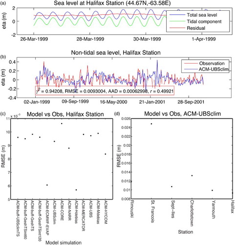
We assessed simulated sea level with respect to observations from coastal station data (with the effect of tides removed, illustrated in Fig. 8a). The time series of sea level at the Halifax station from ACM-UBSclim compares favourably with the observational data for the period 1999–2001, with much of the observed variability captured by the model (RMSE = 0.0093 m; Fig. 8b). All ocean-nesting simulations perform similarly well at the Halifax station, with RMSE values less than 0.01 m (Fig. 8c). Generally, the model represents sea level better at Halifax and Yarmouth than at the Gulf of St. Lawrence and St. Lawrence Estuary stations (Charlottetown, Sept-Îles, and Rimouski), while the model performs worst at the Saint-Francois station situated at the mouth of the St. Lawrence River. This pattern is evident for ACM-UBSclim in Fig. 8d, where with the exception of the Saint-Francois station (RMSE = 0.0248 m), the model simulates sea level variability fairly well (RMSE < 0.014 m). Debiasing HYCOM affected coastal sea levels and improved the fit to observations (RMSE values were reduced at all stations), whereas debiasing MERCATOR produced little effect on sea level (Fig. 8c).

Fig. 8 (a) Time series of the total sea level from the Fisheries and Oceans Canada dataset (blue), the tidal component estimated using T_TIDE from Pawlowicz et al. (2002) (green), and the non-tidal sea level (equivalent to the residual, red) (m) at the Halifax station for a 1-week period starting 26 March 1999. (b) Time series of the non-tidal sea level estimated from the Fisheries and Oceans Canada dataset (red) and in the model simulation ACM-UBSclim (blue) for the time period 1999–2001, with statistical results indicated in the inset (γ², RMSE, the average absolute difference (AAD), and correlation r, following the definitions of γ² and AAD of Zhang and Sheng (2013)). Comparison of RMSE (m) for (c) all simulations at Halifax station, and (d) ACM-UBSclim at all stations (Rimouski, Saint-Francois, Sept-Îles, Charlottetown, Yarmouth, and Halifax).

To summarize, we find the model simulations employing ocean-nesting data from HYCOM or MERCATOR result in a Gulf Stream position too close to the shelf slope, which is associated with poor simulated bottom temperature and salinity and poor simulated current transports. The position of the Gulf Stream in model simulations using UBS data, in contrast, lies within the observed range and current transports close to observed values. Overall, the monthly climatological boundary conditions, UBSclim, provide very similar results to the 5-day varying UBS. ACM-UBSclim is the preferred simulation set-up because of its climatological boundaries, which do not confine the simulation to the specific time period of the parent model.

6 Model assessment III: Effect of nudging in model buffer zone and interior

Although the default set-up in our model does not include nudging in the interior of the model domain, the model is influenced both at its open boundaries and in the 10-grid-cell wide buffer zone adjacent to the open boundaries. In the buffer zone, the model's temperature, salinity, and velocities are nudged toward those of the parent model with a nudging coefficient that decays linearly from 2 day⁻¹ to zero at the 10th interior grid cell. We performed multiple sensitivity experiments to evaluate the treatment of nudging in the model, specifically whether the buffer zone nudging is well configured and whether (and to what extent) applying a weak nudging in the domain interior improves model performance.

We detected only a small effect by varying the buffer zone width (10, 15, and 20 grid cells wide): the Gulf Stream position shifted by approximately 1° (latitude) southward between 58°W and 62°W but was otherwise unaffected (results not shown). Next, to focus on the treatment of buffer zone nudging, we performed two additional experiments: a simulation in which we turned off the nudging of velocities in the buffer zone and only nudged to the parent model's temperature and salinity (referred to as ACM-buff-UBSclimTS), and a simulation in which we nudged in the buffer zone to the Geshelin et al. (1999) climatology instead of the parent model's temperature and salinity (referred to as ACM-buff-GeshTS; note the nudging of buffer zone velocity remained off).

Relative to ACM-UBSclim (which employs the default nudging set-up and was determined to be the simulation that performs best across varied ocean-nesting configurations), turning off nudging to velocity data in the buffer (ACM-buff-UBSclimTS) shifted the Gulf Stream position northward between 62°W and 66°W (Fig. 6b, green line). Replacing the data with climatological temperature and salinity, however, had a large effect; the Gulf Stream in the ACM-buff-GeshTS simulation shifted a large distance southward and was positioned near the centre of the observed range (Fig. 6b, red line).

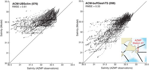
In addition to changing the position of the simulated Gulf Stream, the use of climatological temperature and salinity data in the buffer zone improved the distribution of freshwater in the eastern and central portions of the domain. Time series indicate that SSS improves (relative to climatology) in the Offshore-East, eastern Newfoundland Shelf, Grand Banks, and Gulf of St. Lawrence regions, and bottom temperature and salinity improve in the eastern Newfoundland Shelf and Grand Banks regions. In the statistical assessment of domain-averaged time series (see Table S1c), nudging the temperature and salinity in the buffer zone toward climatology improves the correlations for SSS (from 0.85 to 0.91), bottom temperature, and salinity. At the same time, the RMSE values increase slightly (SST by 0.17°C and SSS by 0.05, bottom temperature and salinity by 0.06°C and 0.02, respectively). Simulated volume transport improves greatly from ACM-buff-UBSclim (Fig. 7c, light blue line) to ACM-buff-GeshTS (Fig. 7c, green line) for both the Labrador Current (at LC1, GB1, and GB2) and the NSC and Shelf Break Current (at SF2). Simulated sea level at coastal stations remains generally unaffected (e.g., Fig. 8c). At AZMP Station 27, located off the southeast coast of Newfoundland, modelled salinity improves (relative to AZMP salinity observations during the 1999–2004 period) throughout the water column (Fig. 9); RMSE decreases from 0.61 (ACM-UBSclim) to 0.33 (ACM-buff-GeshTS). We conclude that the choice of temperature and salinity data for nudging in the buffer zone can have a sizeable effect, and in this case using the climatological data improved model performance.

Fig. 9 Simulated and observed salinity at AZMP Station 27 (indicated on inset map) for the period 1999–2004. Root-mean-square error (RMSE) is reported for ACM-UBSclim (left) and ACM-buffGeshTS (right).

Applying a weak or moderate nudging (corresponding to a 120-day and 60-day time scale) of temperature and salinity to climatology in the model domain's interior improves surface salinity and subsurface temperature and salinity evaluated by the domain-averaged RMSE and R² (see Table S1c). which is not unexpected because these time series are compared with climatological data. The improvement is rather small in most areas, probably because the corresponding simulation without interior nudging is already performing well (ACM-buffGeshTS). There is no improvement in SST likely because it is already very well simulated without interior nudging. Examination of monthly-mean surface velocities suggests that interior nudging affects circulation features throughout the domain, especially in the interior of the model domain. The simulated Halifax section (SF2) volume transport is improved with the application of interior nudging (Fig. 7c). Moderate interior nudging is associated with a slightly weaker Gaspé Current in the Gulf of St. Lawrence, weaker outflow through Cabot Strait, and a weaker NSC, but a somewhat enhanced shelf break current, and less Gulf Stream variability (though the Gulf Stream mean position and coastal sea levels are essentially unchanged, as determined by the GSNW index and tide-gauge analysis (Fig. 8c), respectively). Little to no improvement is found in the simulated Labrador Current volume transport at LC1 or Flemish Pass (GB1) with the application of interior nudging.

7 Model assessment IV: Effect of expanding the model domain

It is questionable whether the original model domain is optimally situated because its boundaries intersect a major topographical feature, Flemish Cap, and lie very near the edge of the Newfoundland Shelf and the Tail of the Grand Banks (see regional topography in Fig. 1). We implemented the model in an expanded domain (300-by-150 grid cells in the horizontal) in which the southern and eastern boundaries have been moved southward and eastward, to resolve the Flemish Cap topography. The eastern and southern boundaries in this larger domain are located in deep water (>3000 m) (Fig. 10a). The expanded domain has a slightly higher horizontal resolution and a steeper bathymetry. We performed simulations ACM-original (the same simulation as ACM-UBSclim) and ACM-large (Table 2) to assess the influence of the model domain expansion on the ACM.

Fig. 10 (a) Model domain with bathymetry (m) for original and large grids, and (b) time series of area-averaged Scotian Shelf properties T (left) and S (right) at sea surface (upper) and bottom (lower) from model simulations ACM-orig (pink) and ACM-large (black), with comparison to climatology (grey dashed line) and AVHRR satellite SST (grey stars).

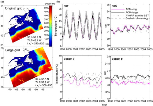
Time series of area-averaged temperature and salinity on the Scotian Shelf show a very similar evolution at the sea surface, but in the large domain bottom water on the Scotian Shelf warms and becomes more saline (Fig. 10b). As summarized in Table S1d, statistical evaluation of these properties across sub-areas of the model reveals a similar pattern. Expanding the model domain does not cause important changes to the expression of surface temperature and salinity, but bottom temperature and salinity are affected. In bottom temperature, ACM-large has a slightly improved RMSE (0.18°C compared with 0.20°C in ACM-orig) and R² value (0.84 compared with 0.73 in ACM-orig), whereas for bottom salinity, ACM-orig performs better.

Circulation differences between the original and large model domains are apparent in plots of monthly-mean surface velocity in January and April 2003 (Fig. 11). Although the NSC is similar across domains, in the larger domain there is a slight weakening around the Tail of the Grand Banks and a weaker outflow through Cabot Strait. Finally, the largest differences are seen in the shelf break current, which is well defined in April in the original domain, while there is no coherent velocity structure to provide evidence of this key feature in the large domain. Compared with the Loder et al. (1998) volume transports, ACM-large (Fig. 7c, magenta line) outperforms ACM-original (Fig. 7c, blue line) at all four sections. The Labrador Current is stronger at LC1 and Flemish Pass, while transport is weaker at the Tail of the Grand Banks (GB2) and the Halifax section (SF2). The long-term mean GSNW position in ACM-large varies within 0.5° of latitude from the ACM-original position (not shown). The time-evolution of surface velocity (not shown) indicates that the Gulf Stream has greater variability (e.g., more meandering) across the southern portion of the large domain.

Fig. 11 Monthly-mean surface velocity (m s⁻¹) in ACM-original (top) and ACM-large (bottom) in January 2003 (left) and April 2003 (right).

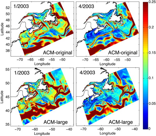
There are several potential explanations for the circulation differences between the original and large domains. First, in the original domain, the Gulf Stream and the shelf-edge branch of the Labrador Current are imposed along the northern portion of the eastern boundary and the eastern portion of the southern boundary. These large-scale currents are tightly defined through the boundary conditions and the buffer zone adjacent to open boundaries. In contrast, in the large domain these currents are only defined for the width of the incoming current in the northern and western boundaries (for the Labrador Current and Gulf Stream, respectively). In the large domain the model's internal dynamics, therefore, play a larger role in the evolution of each current away from the boundaries, which in turn permits more variability in these key currents. Second, the large domain has an incrementally higher horizontal resolution and an increased bathymetry steepness. It is possible that the changes in resolution and bathymetry contribute to the observed circulation differences.

8 Conclusions

In our model simulations forced with either NARR or ECMWF surface forcing, simulated SST is in good agreement with observations, while the simulation forced with ECMWF agrees better with observed SSS than the one forced by NARR. Prescribing evaporation using ECMWF data did not improve model salinity. CORE surface forcing leads to poor SSS representation and cooler modelled SST, resulting in sizeable misfit and bias relative to the observations.

Using initial and boundary information from the global MERCATOR and HYCOM models produced the worst results of all our model simulations. Debiasing these ocean model datasets did not improve SST, and the time series of SSS achieved a better fit to climatological values only in the easternmost portion of the domain. Although debiasing led to improved bottom temperature for both HYCOM and MERCATOR, bottom salinity was only slightly improved in a few regions (in the Grand Banks and eastern Newfoundland Shelf for MERCATOR and in the Offshore regions and the eastern Newfoundland Shelf for HYCOM). We conclude that debiasing (i.e., replacing temperature and salinity monthly-mean values with those from climatology) of global ocean parent models does not guarantee model improvement.

Model simulations employing initial and boundary information constructed from the larger scale regional model of Urrego-Blanco and Sheng (2012; UBS) outperformed simulations nested in global ocean parent models. ACM-UBSclim using long-term, monthly-mean UBS data performed as well as ACM-UBS and is the preferred simulation because of its climatological boundary conditions.

Additional sensitivity experiments focused on the treatment of nudging in the buffer zone adjacent to open boundaries. These experiments revealed that nudging velocities in the buffer zone was not important in the model but that the choice of temperature and salinity data had a large effect. By nudging temperature and salinity in the buffer zone to climatology instead of UBSclim, the Gulf Stream position shifted southward to the centre of the observed range, and salinity in the eastern portion of the domain was much improved. Applying weak (120-day) or moderate (60-day) nudging in the model domain interior appeared to improve the distribution of temperature and salinity further and affected regional currents (improving some features and worsening others).

Expanding the model domain to the east and south to resolve Flemish Cap and increase the distance between model boundaries and topographical gradients had little effect on sea surface properties but had a larger effect on the model's bottom level. On the Scotian Shelf, bottom temperature and salinity increased compared with the original domain. Important differences emerged with respect to key circulation features, for example, in the large domain the surface expression of the shelf break current was less evident, coupled with a weaker Cabot Strait outflow, and a more variable (meandering) Gulf Stream than in the original domain.

This work presents an investigation of the impacts of model configuration choices on model performance. Perhaps especially because our regional model is situated in a complex coastal environment, influenced by large current systems from the north (Labrador Current) and the south (Gulf Stream), model configuration choices can greatly affect model results. We assessed 3.5 surface forcing datasets, six ocean model nesting choices, two model grids, and various types of nudging to climatology in the buffer zone and model interior for the years 1999–2004. We expect the model is capable of reproducing other time periods; for example, corresponding to different North Atlantic Oscillation states, provided appropriate surface forcing and boundary conditions are applied, though this has not been investigated in this study. In addition to optimizing our own model's configuration and performance, our results provide useful guidance in model development and testing of other regional ocean models, both within the northwest North Atlantic and beyond.

Supplemental data

Supplemental data for this article can be accessed at http://dx.doi.org//10.1080/07055900.2016.1147416.

Acknowledgements

We thank Christoph Renkl for his contributions to the preparation of surface forcing data and model assessment scripts. We thank Kyoko Ohashi for her advice on the implementation of rivers in the model. We are grateful to Wei Chen for extracting the sea level data and performing analyses. We also thank Rui Zhang for his assistance in evaluating model currents.

Disclosure statement

No potential conflict of interest was reported by the authors.

ORCID

Catherine E. Brennan http://orcid.org/0000-0003-2593-7222

Laura Bianucci http://orcid.org/0000-0002-4492-8930

Katja Fennel http://orcid.org/0000-0003-3170-2331

Additional information

Funding

We acknowledge funding by the Marine Environmental Observation Prediction and Response Network (MEOPAR).

References

- Anderson, C., & Smith, P. C. (1989). Oceanographic observations on the Scotian shelf during CASP. Atmosphere-Ocean, 27, 130–156. doi: 10.1080/07055900.1989.9649331
- Barnier, B., & Ferry, N. (2011). GLobal Ocean Reanalyses and Simulations: GLORYS2V1 product scientific and technical notice for users. Technical notice version 1. Mercator-Ocean, Ramonville-Saint-Ange, France.
- Barnier, B., Madec, G., Penduff, T., Molines, J.-M., Treguier, A.-M., Le Sommer, J., … De Cuevas, B. (2006). Impact of partial steps and momentum advection schemes in a global ocean circulation model at eddy permitting resolution. Ocean Dynamics, 56, 543–567. doi:10.1007/s10236-006-0082-1
- Cummings, J. A. (2005). Operational multivariate ocean data assimilation. Quarterly Journal of the Royal Meteorological Society, 131(613), 3583–3604. doi: 10.1256/qj.05.105
- Dee, D. P., Uppala, S. M., Simmons, A. J., Berrisford, P., Poli, P., Kobayashi, S., … Vitart, F. (2011). The ERA-Interim reanalysis: Configuration and performance of the data assimilation system. Quarterly Journal of the Royal Meteorological Society, 137, 553–597. doi:10.1002/qj.828
- Fairall, C. W., Bradley, E. F., Godfrey, J. S., Wick, G. A., Edson, J. B., & Young, G. S. (1996). Cool-skin and warm-layer effects on sea surface temperature. Journal of Geophysical Research, 101, 1295–1308. doi: 10.1029/95JC03190
- Fairall, C. W., Bradley, E. F., Rogers, D. P., Edson, J. B., & Young, G. S. (1996). Bulk parameterization of air-sea fluxes for tropical ocean global atmosphere coupled-ocean atmosphere response experiment. Journal of Geophysical Research, 101, 3747–3764. doi: 10.1029/95JC03205
- Fisheries and Oceans Canada. (2011). Hydrographic data: Stations and sections of AZMP [Data]. Retrieved from http://www.meds-sdmm.dfo-mpo.gc.ca/isdm-gdsi/azmp-pmza/hydro/index-eng.html
- Fisheries and Oceans Canada. (2015). Canadian station inventory and data download. Retrieved from http://www.isdm-gdsi.gc.ca/isdm-gdsi/twl-mne/maps-cartes/inventory-inventaire-eng.asp
- Geshelin, Y., Sheng, J., & Greatbatch, R. J. (1999). Monthly mean climatologies of temperature and salinity in the western North Atlantic. Canadian Data Report of Hydrography and Ocean Sciences, 153, Dartmouth, Nova Scotia, Canada: Bedford Institute of Oceanography.
- Government of Canada. (2015). Wateroffice: Historical hydrometric data search [Data]. Retrieved from the Water Survey of Canada website http://wateroffice.ec.gc.ca/search/search_e.html?sType=h2oArc
- Griffies, S. M., Winton, M., & Samuels, B. L. (2004). The Large and Yeager (2004) dataset and CORE. CORE release notes. Retrieved from http://data1.gfdl.noaa.gov/nomads/forms/mom4/CORE/doc.html
- Guo, L., Perrie, W., Long, Z., Chassé, J., Zhang, Y., & Huang, A. (2013). Dynamical downscaling over the Gulf of St. Lawrence using the Canadian Regional Climate Model. Atmosphere-Ocean, 51(3), 265–283. doi:10.1080/07055900.2013.798778
- Haidvogel, D. B., Arango, H., Budgell, W. P., Cornuelle, B. D., Curchitser, E., Di Lorenzo, E., … Wilkin, J. (2008). Regional ocean forecasting in terrain-following coordinates: Model formulation and skill assessment. Journal of Computational Physics, 227, 3595–3624. doi:10.1016/i.jcp.2007.06.016
- Han, G. (2000). Three-dimensional modeling of tidal currents and mixing quantities over the Newfoundland shelf. Journal of Geophysical Research, 105, 11407–11422. doi: 10.1029/2000JC900033
- Han, G. (2005). Wind-driven barotropic circulation off Newfoundland and Labrador. Continental Shelf Research, 25, 2084–2106. doi:10.1016/j.csr.2005.04.015
- Han, G., & Loder, J. W. (2003). Three-dimensional seasonal-mean circulation and hydrography on the eastern Scotian shelf. Journal of Geophysical Research, 108, 1–21. doi:10.1029/2002JC001463
- Han, G., Lu, Z., Wang, Z., Helbig, J., Chen, N., & de Young, B. (2008) Seasonal variability of the Labrador Current and shelf circulation off Newfoundland. Journal of Geophysical Research, 113, C10013. doi:10.1029/2007JC004376
- Joyce, T. M., Deser, C., & Spall, M. A. (2000). The relation between decadal variability of subtropical model water and the North Atlantic Oscillation. Journal of Climate, 13, 2550–2569. doi: 10.1175/1520-0442(2000)013<2550:TRBDVO>2.0.CO;2
- Kilpatrick, K. A., Podesta, G. P., & Evans, R. (2001). Overview of the NOAA/NASA Advanced Very High Resolution Radiometer Pathfinder algorithm for sea surface temperature and associated matchup database. Journal of Geophysical Research: Oceans, 106(C5), 9179–9197. doi: 10.1029/1999JC000065
- Large, W. G., & Yeager, S. G. (2004). Diurnal to decadal global forcing for ocean and sea-ice models: The data sets and flux climatologies. CGD Division of the National Center for Atmospheric Research, NCAR Technical Note: NCAR/TN-460+STR. Boulder, CO: NCAR.
- Lazier, J. R. N., & Wright, D. G. (1993). Annual variations in the Labrador Current. Journal of Physical Oceanography, 23, 659–678. doi: 10.1175/1520-0485(1993)023<0659:AVVITL>2.0.CO;2
- Liu, W. T., Katsaros, K. B., & Businger, J. A. (1979). Bulk parameterization of the air-sea exchange of heat and water vapor including the molecular constraints at the interface. Journal of Atmospheric Science, 36, 1722–1735. doi: 10.1175/1520-0469(1979)036<1722:BPOASE>2.0.CO;2
- Loder, J. W., Petrie, B., & Gawarkiewicz, G. (1998). The coastal ocean off northeastern North America: A large-scale view. In A. R. Robinson & K. H. Brink (Eds.), The sea. Vol 11, The global coastal ocean: Regional studies and syntheses (pp. 105–133). New York, USA: John Wiley & Sons, Inc.
- Marchesiello, P., McWilliams, J. C., & Shchepetkin, A. F. (2001). Open boundary conditions for long-term integration of regional ocean models. Ocean Modelling, 3, 1–20. doi: 10.1016/S1463-5003(00)00013-5
- Mesinger, F., DiMego, G., Kalnay, E., Mitchell, K., Shafran, P. C., Ebisuzaki, W., … Shi, W. (2006). North American regional reanalysis. Bulletin of the American Meteorological Society, 87, 343–360. doi:10/1175/BAMS-87-3-343.
- Pawlowicz, R. (2011). T_Tide harmonic analysis toolbox. Retrieved from https://www.eoas.ubc.ca/~rich/#T_Tide
- Pawlowicz, R., Beardsley, B., & Lentz, S. (2002). Classical tidal harmonic analysis including error estimates in MATLAB using T_TIDE. Computers and Geosciences, 28, 929–937. doi: 10.1016/S0098-3004(02)00013-4
- Petrie, B., & Buckley, J. (1996). Transport and freshwater flux of the Labrador Current in flemish pass. Journal of Geophysical Research, 101, 28335–28342. doi: 10.1029/96JC02779
- Petrie, B. D., & Drinkwater, K. (1993). Temperature and salinity variability on the Scotian Shelf and in the Gulf of Maine 1945–1990. Journal of Geophysical Research, 98, 20079–20089. doi: 10.1029/93JC02191
- Pham, D. T., Verron, J., & Roubaud, M. C. (1998). A singular evolutive extended Kalman filter for data assimilation in oceanography. Journal of Marine Systems, 16(3), 323–340. doi: 10.1016/S0924-7963(97)00109-7
- Therriault, J.-C., Petrie, B., Pepin, P., Gagnon, J., Gregory, D., Helbig, J., … Sameoto, D. (1998). Proposal for a Northwest Atlantic zonal monitoring program. Canadian Technical Report of Hydrography and Ocean Sciences, 194. Retrieved from http://www.dfo-mpo.gc.ca/Library/224076.pdf
- Thompson, K. R., Loucks, R. H., & Trites, R. W. (1988). Sea surface temperature variability in the shelf-slope region of the northwest Atlantic. Atmosphere-Ocean, 26, 292–299. doi: 10.1080/07055900.1988.9649304
- Tranchant, B., Testut, C.-E., Renault, L., Ferry, N., Birol, F., & Brasseur, P. (2008). Expected impact of the future SMOS and Aquarius Ocean surface salinity missions in the Mercator Ocean operational systems: New perspectives to monitor the ocean circulation. Remote Sensing of Environment, 112, 1476–1487. doi: 10.1016/j.rse.2007.06.023
- Umlauf, L., & Burchard, H. (2003). A generic length-scale equation for geophysical turbulence models. Journal of Marine Research, 61, 235–265. doi: 10.1357/002224003322005087
- Urrego-Blanco, J., & Sheng, J. (2012). Interannual variability of the circulation over the eastern Canadian Shelf. Atmosphere-Ocean, 50, 277–300. doi:10.1080/07055900.2012.680430
- Warner, J. C., Sherwood, C. R., Arango, H. G., & Signell, R. P. (2005). Performance of four turbulence closure models implemented using a generic length scale method. Ocean Modelling, 8, 81–113. doi:10.1016/j.ocemod.2003.12.003
- Wilkin, J. L., & Hunter, E. J. (2013). An assessment of the skill of real-time models of Mid-Atlantic Bight continental shelf circulation. Journal of Geophysical Research: Oceans, 118, 2919–2933. doi:10.1002/jgrc.20223
- Zhang, H., & Sheng, J. (2013). Estimation of extreme sea levels over the eastern continental shelf of North America. Journal of Geophysical Research: Oceans, 118, 6253–6273. doi:10.1002/2013JC009160