Simulation and Regionalization of Daily Global Solar Radiation: A Case Study in Quebec, Canada

Abstract

Global solar radiation (GSR) is essential for agricultural and plant growth modelling, air and water heating analyses, and solar electric power systems. However, GSR gauging stations are scarce compared with stations for monitoring common meteorological variables such as air temperature and relative humidity. In this study, one power function, three linear regression, and three non-linear models based on an artificial neural network (ANN) are developed to extend short records of daily GSR for meteorological stations where predictors (i.e., temperature and/or relative humidity) are available. The seven models are then applied to 19 meteorological stations located across the province of Quebec (Canada). On average, the root-mean-square errors (RMSEs) for ANN-based models are 0.33–0.54 MJ m⁻² d⁻¹ smaller than those for the power function and linear regression models for the same input variables, indicating that the non-linear ANN-based models are more efficient in simulating daily GSR. Regionalization potential of the seven models is also evaluated for ungauged stations where predictors are available. The power function and the three linear regression models are tested by interpolating spatially correlated at-site coefficients using universal kriging or by applying a leave-one-out calibration procedure for spatially uncorrelated at-site coefficients. Regional ANN-based models are also developed by training the model based on the leave-one-out procedure. The RMSEs for regional ANN models are 0.08–0.46 MJ m⁻² d⁻¹ smaller than for other models using the same input conditions. However, the regional ANN-based models are more sensitive to new station input values compared with the other models. Maps of interpolated coefficients and regional equations of the power function and the linear regression models are provided for direct application to the study area.

Résumé

[Traduit par la rédaction] La mesure du rayonnement solaire global s'avère essentielle à la modélisation de paramètres agricoles ou de la croissance des plantes, ainsi qu'aux analyses de réchauffement de l'eau et de l'air, et aux systèmes d'alimentation à l’énergie solaire. Toutefois, les stations de mesure du rayonnement global demeurent rares en comparaison avec les stations fournissant les variables météorologiques habituelles comme la température de l'air ou l'humidité relative. Nous élaborons dans cette étude une fonction de puissance, trois équations de régression linéaire et trois modèles non linéaires fondés sur un réseau de neurones artificiels, afin d'enrichir les courts relevés quotidiens de rayonnement global, aux sites où les prédicteurs nécessaires (température ou humidité relative) existent. Nous appliquons ces sept modèles à 19 stations météorologiques situées partout dans la province de Québec (Canada). En moyenne, l'erreur-type de nos modèles neuronaux est de 0,33 à 0,54 MJ m^-2 j^-1 inférieure à celle de la fonction de puissance et des équations de régression linéaire, et ce, pour les mêmes variables entrantes. Les modèles non linéaires qui utilisent des réseaux neuronaux semblent donc les plus efficaces pour simuler le rayonnement global quotidien. Nous évaluons aussi le potentiel d'expansion spatiale des sept modèles pour les stations où seuls les prédicteurs existent. Nous testons la fonction de puissance et les trois équations de régression linéaire en interpolant les coefficients spatialement corrélés au site à l'aide d'un krigeage universel, ou en appliquant une validation croisée (exclusion tour à tour) pour les coefficients non spatialement corrélés au site. Nous élaborons aussi des modèles neuronaux régionaux en entraînant le modèle selon une procédure d'exclusion tour à tour. L'erreur-type des modèles neuronaux régionaux est de 0,08 à 0,46 MJ m^-2 j^-1 inférieure à celle des autres modèles qui utilisent les mêmes conditions entrantes. Toutefois, les modèles neuronaux régionaux sont plus sensibles à l'introduction de valeurs issues de nouvelles stations que les autres modèles. Nous incluons des cartes de coefficients interpolés et des équations de la fonction de puissance, ainsi que les modèles de régression linéaire pour application directe à la zone d’étude.

KEYWORDS:

•  global solar radiation
• regionalization
• stochastic model
• temperature
• relative humidity

1 Introduction

Global solar radiation (GSR) data are essential for many applications, such as agricultural and plant growth modelling, air and water heating analyses, and solar electric power systems. In particular, GSR data were needed for a study on lake thermal habitats on a north–south section across the province of Quebec (Bélanger et al., 2013; Bélanger et al., unpublished manuscript, 2015). However, meteorological stations measuring GSR are more scarce than those measuring common meteorological variables, such as air temperature, precipitation, and relative humidity. Furthermore, observational records of GSR are usually short and often have missing data because of equipment malfunction (Cutforth & Judiesch, 2007).

Physical or stochastic simulation models are generally used for substituting missing values and extending short record lengths of the GSR at measuring stations (see Tymvios, Jacovides, Michaelides, and Scouteli (2005) and Fortin, Anctil, Parent, and Bolinder (2008) for more details). Physical models are based on complex physical interactions between the GSR and the terrestrial atmosphere, such as Rayleigh scattering, radiative absorption by ozone and water vapour, and aerosol extinction (e.g., De La Casiniere, Bokoye, & Cabot, 1997; Gueymard, 1989; Leckner, 1978). Stochastic models are based on empirical relationships between the GSR and the other correlated meteorological variables, such as sunshine hours, temperature, and relative humidity (e.g., Benghanem, Mellit, & Alamri, 2009; Fortin et al., 2008; Liu et al., 2009; Mahmood & Hubbard, 2002; Trnka, Žalud, Eitzinger, & Dubrovský, 2005; Tymvios et al., 2005; Weiss & Hays, 2004). Stochastic models are frequently selected because they are relatively simple to develop and require fewer input variables than physical models (Fortin et al., 2008; Tymvios et al., 2005). This study is focused on stochastic models.

Linear and non-linear regression models are the main tools used to drive empirical relationships between the common meteorological variables and the GSR in a stochastic model (e.g., Behrang, Assareh, Noghrehabadi, & Ghanbarzadeh, 2011; Benghanem et al., 2009; De Jong & Stewart, 1993; Fortin et al., 2008; Jiang, 2008; Liu et al., 2009; Mahmood & Hubbard, 2002; Mubiru & Banda, 2008; Podestá, Núñez, Villanueva, & Skansi, 2004; Rivington, Bellocchi, Matthews, & Buchan, 2005; Trnka et al., 2005; Tymvios et al., 2005; Weiss & Hays, 2004). Recently, artificial neural networks (ANN) have also been employed as transfer functions between the GSR and the independent variables (Benghanem et al., 2009; Fortin et al., 2008; Jiang, 2008; Mubiru & Banda, 2008; Tymvios et al., 2005). Several studies (Benghanem et al., 2009; Fortin et al., 2008; Jiang, 2008; Mubiru & Banda, 2008; Tymvios et al., 2005) reported that ANN models can perform better than regression-based models because they generally drive robust (probably non-linear) relationships between input and output variables, even though they are computationally expensive and complex compared with the latter.

Sunshine duration is known as the best predictor for monthly (e.g., Behrang et al., 2011; Ertekin & Evrendilek, 2007; Hussain, Rahman, & Rahman, 1999; Jiang, 2008; Mubiru & Banda, 2008; Tymvios et al., 2005) and daily (e.g., Benghanem et al., 2009; Podestá et al., 2004; Rivington et al., 2005; Trnka et al., 2005) stochastic GSR simulations. Sunshine duration, however, has not been recorded since 1999 at almost all meteorological stations in Canada because of the difficulty in measuring it (Cutforth & Judiesch, 2007). Cloud cover can also be considered a predictor variable for GSR. Several studies have formulated stochastic GSR models using cloud cover as a predictor (e.g., Gul, Muneer, & Kambezidis, 1998; Nimnuan & Janjai, 2012). However, Gul et al. (1998) reported that a stochastic model based on sunshine duration and temperatures performs better than one based on cloud-cover information because the former predictors are recorded more rigorously, whereas cloud cover is often based on visual estimates. Temperature is commonly employed to simulate GSR although it has a weaker correlation with GSR than sunshine duration (Abraha & Savage, 2008; Benghanem et al., 2009; Bristow & Campbell, 1984; De Jong & Stewart, 1993; Fortin et al., 2008; Liu et al., 2009; Mahmood & Hubbard, 2002; Podestá et al., 2004; Rivington et al., 2005; Trnka et al., 2005; Weiss & Hays, 2004). In addition, relative humidity has occasionally been employed to simulate daily GSR (Benghanem et al., 2009; Mubiru & Banda, 2008).

Estimates of GSR at ungauged stations that measure other meteorological variables can be simulated using a regional GSR model. The calibratation of this model is based on all available GSR and meteorological observations for the region of interest, which allows for the simulation of GSR at ungauged stations where covariables are available. However, in the past, regionalization studies have rarely been conducted using stochastic GSR models. Hunt, Kuchar, and Swanton (1998) applied a stochastic GSR model using daily temperature as a covariable in Ontario, Canada, and reported that their model can be applied to an ungauged station located less than 390 km away. Weiss and Hays (2004) suggested an equation to predict the coefficients of their stochastic GSR model, using annual means of daily diurnal temperature range (DTR) of a station of interest. Miller, Rivington, Matthews, Buchan, and Bellocchi (2008) tested the ability to regionalize their stochastic model by interpolating the model's coefficients using the ordinary kriging method and reported that the regionalization performances were acceptable for their study area (i.e., United Kingdom). Liu et al. (2009) derived relationships between stochastic model coefficients and domain factors (i.e., latitude, longitude, and altitude) based on 15 stations in China.

The present study compares one power function, three linear regression, and three non-linear ANN-based stochastic models to simulate daily GSR using two meteorological input variables (i.e., daily temperature and relative humidity). The seven models are applied to 19 meteorological stations located across the province of Quebec, Canada (45.1°–58.5°N, 64.2°–79.0°W). Additionally, the regionalization potential of the seven models is evaluated for the study area. In the process, coefficients of the power function and linear regression models are interpolated and presented using a geostatistical technique (i.e., universal kriging). Similarly, the regional ANN models are trained by observation datasets of all available stations in the study region. Finally, regionalization performances among the power function, linear regression, and ANN-based approaches are discussed.

2 Methodologies

a Stochastic GSR Models

Hargreaves and Samani (1982) suggested a regression-based GSR model using daily DTR as a predictor. It assumes that the solar transmissivity (i.e., the ratio of incoming GSR on the horizontal surface of the earth () to solar irradiation on the horizontal surface at the top of the atmosphere ()) on a given day is proportional to the power transformed daily DTR as follows:(1)

where and (Kelvin) are the daily maximum and minimum temperatures in a given day, and and are empirical coefficients that are estimated using a non-linear least squares approach. The incoming solar radiation at the top of the atmosphere () is a function of latitude and Julian day of a site and is estimated using the standard geometric method provided by Sellers (1965). The simulated GSR value is . This model is called “HS(T)” in this study. The details of this method are also provided by Fortin et al. (2008).

Benghanem et al. (2009) applied simple and multiple linear regression models to simulate daily solar transmissivity, using the ratio of daily minimum and maximum temperatures () and/or daily relative humidity as predictors. In this study, three linear regression models are developed using the daily temperature ratio and relative humidity as follows:(2) (3) (4)

where is the mean daily relative humidity and , , and are the regression coefficients of each model. The coefficients are estimated by an ordinary least squares estimation. The units of the daily maximum and minimum temperatures are Kelvin, in order to avoid negative value effects, and daily relative humidity is given as a percentage. The three models are called LR(T), LR(H), and LR(TH), respectively in this study.

Feed-forward ANNs have been employed recently to simulate GSR (Benghanem et al., 2009; Fortin et al., 2008; Mubiru & Banda, 2008; Tymvios et al., 2005) and diffuse solar radiation (Jiang, 2008) using meteorological input variables. This study employs a three-layer feed-forward ANN model, which includes a set of computation nodes for each of the input, hidden (single), and output layer. The Bayesian regularization backpropagation (BRBP) algorithm is used to train the ANN model. The BRBP is a network training function that updates the weight and bias values according to the Levenberg–Marquardt optimization technique (Haykin, 1994). The BRBP algorithm minimizes a combination of the squared error and the number of ANN model parameters to train in order to produce stable outputs for new input data (i.e., to avoid overfitting). A hyperbolic tangent sigmoid function and a linear function are used, respectively, at the hidden layer and the output layer nodes; detailed descriptions of these activation functions are provided in Haykin (1994). The current study develops the following three ANN GSR simulation models:(5) (6) (7)

where ANN is the three-layer feed-forward ANN trained by the BRBP algorithm. The three models are called ANN(T), ANN(H), and ANN(TH) in the present study. An important issue in ANN modelling is the determination of the number of hidden nodes. Fletcher and Goss (1993) stated that the optimal number of hidden nodes is generally within (2p^0.5 + o) – (2p + 1), where p and o represent the number of predictor and predictand variables, respectively. This study selected 4, 3, and 5 hidden nodes for the ANN(T), ANN(H), and ANN(TH) models, respectively, based on a trial-and-error procedure. Therefore, ANN(T), ANN(H), and ANN(TH) have 16, 9, and 25 weights, respectively, which determine the strength of the connections between the input nodes and the hidden nodes as well as between the hidden nodes and the output nodes.

b Kriging and Regionalization

Kriging is a geostatistical estimation technique based on the linear least squares estimation algorithm. The method estimates the value at an unobserved location from observations of the random field at locations . Ordinary kriging is the most common type of kriging. The estimation of the ordinary kriging at a location is given by:(8)

where are the weights of the ordinary kriging that fulfill the unbiased condition . The weights are calculated by the ordinary kriging equation system:(9)

where is a Lagrangian parameter employed to minimize the kriging error under the unbiasedness condition, and is a variogram function used to quantify the spatial dependence as a function of inter-station distance (i.e., between and ). There are several variogram functions, such as exponential, Gaussian, and spherical models, but this study uses the Gaussian variogram model following a trial-and-error examination. Universal kriging is a general case of ordinary kriging, which assumes is a general polynomial trend model of the following form:

where are known independent variables for the trend estimation. Detailed descriptions of variogram functions as well as ordinary and universal kriging approaches can be found in Isaaks and Srivastava (1989) and Goovaerts (1997).

To verify the interpolation performances of the kriging approaches, a leave-one-out cross-validation method is adopted (i.e., among the n observation stations, , , is interpolated using the remaining n−1 stations). This interpolation is repeated for all the observation stations, and the interpolated is compared with the associated observation . In this study, ordinary and universal kriging methods are tested to interpolate coefficients of the HS(T) and the three linear models. The results are presented for models with parameters interpolated using a leave-one-out approach that show statistically significant positive linear correlations with the at-site estimated parameters according to a Student's t-test at the 95% confidence level. However, if this condition is not respected, the coefficients of the regional regression-based models are estimated using a leave-one-out calibration procedure. The latter implies that at a given station, the regional regression-based models are calibrated by using observations from all the remaining stations for the calibration period, which is repeated for all stations. Similarly, the leave-one-out approach is applied to train the regional ANN-based models. The trained models are then evaluated at each station by simulating daily GSR series. In the regional ANN models, mean GSR varies with , which is a function of the latitude of each station.

c Model Evaluation Measures

Model performances are evaluated by the mean bias error (MBE), root-mean-square error (RMSE), r² (coefficient of determination). The MBE and RMSE are defined as follows:(10) (11)

where and are observed and simulated values, respectively, and is the record size; r² is the squared value of the (Pearson's product-moment) linear correlation coefficient between observed and simulated values. It provides the proportion of explained variance of the observations by an applied model and is defined by the following equation:(12)

where is the mean of the observed values.

3 Study area and data

Daily GSR, maximum and minimum temperatures, as well as mean relative humidity are obtained from 19 Environment Canada meteorological stations located between latitude 45.1°N and 58.5°N and longitude 64.2°W and 79.0°W. Figure 1 presents the locations of the 19 stations across the province of Quebec in eastern Canada. The southern part of Quebec, which is the most populated area in the province, has a high density of observation stations. Observation stations measuring daily temperature and humidity are presented in the figure if they have more than 50% of available data for the common analysis period (2003–2010). As mentioned before, many meteorological stations have only daily temperature and/or relative humidity data. Therefore, the stations without GSR observations can be estimated by applying a regional GSR simulation model.

Fig. 1 Map of eastern Canada and the meteorological stations in the province of Quebec. Selected GSR stations are represented by a blue circle with their identification number. Daily temperature and relative humidity observation stations are marked by a red + and black × symbols, respectively, when they have less than 50% missing data for the common analysis period (from 2003 to 2010).

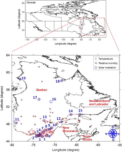
Table 1 presents the station identification number, location information (latitude, longitude, and altitude), analysis periods (calibration and validation), and the annual average GSR during their respective analysis periods; the stations are sorted in ascending order of latitude. Generally, values of the annual average GSR decrease as station latitude increases; however, stations 1, 4, and 11, which are at a relatively high altitude, show smaller annual average GSR than nearby stations. It is notable that the four stations located in northern Quebec were chosen to ensure a minimal spatial density of observation stations; however, their analysis periods are different from the 2003–2010 common period.

Table 1. The 19 observation stations selected for this study showing station identification number, location information (latitude, longitude, and altitude), analysis periods (calibration and validation), and annual average of daily GSR for the analysis periods.

No.	Station No.	Latitude (^oN)	Longitude (^oW)	Altitude (m)	Calibration Period	Validation Period	Annual Average GSR (MJ m^−2 d^−1)
1	7022579	45.05	72.86	152.4	2003–2008	2009–2010	11.54
2	702FQLF	45.12	74.29	49.1	2003–2008	2009–2010	12.81
3	702LED4	45.29	73.35	43.8	2003–2008	2009–2010	13.24
4	7024280	45.37	71.82	181.0	2003–2008	2009–2010	11.63
5	702S006	45.47	73.74	32.1	2003–2008	2009	12.51
6	702327X	45.72	73.38	17.9	2003–2008	2009–2010	13.08
7	7025442	46.23	72.66	8.0	2003–2008	2009–2010	12.57
8	7011983	46.69	71.97	61.0	2003–2008	2009–2010	12.24
9	701Q004	46.78	71.29	91.4	2003–2008	2009–2010	11.06
10	7041JG6	47.08	70.78	6.0	2003–2008	2009–2010	11.91
11	7086716	48.25	79.03	318.0	2003–2008	2009–2010	11.77
12	7056068	48.51	68.47	4.9	2003–2008	2009–2010	12.31
13	7065639	48.84	72.55	137.2	2003–2008	2009–2010	12.77
14	7047912	50.22	66.25	53.1	2003–2007	2008	11.19
15	7044328	50.27	64.23	11.0	2003–2008	2009–2010	11.06
16	7095480	53.20	70.90	536.1	1977–1982	1983–1984	11.19
17	7093GJ3	53.76	73.68	306.3	1987–1992	1993–1994	10.94
18	7113E37	58.10	68.42	39.3	1987–1992	1993–1994	10.29
19	7103282	58.47	78.08	24.4	1985–1990	1991–1992	10.92

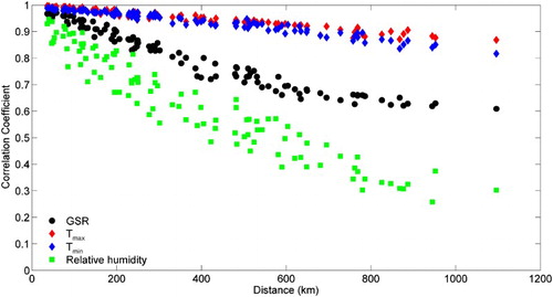
Figure 2 shows the spatial dependence structures of the GSR and the predictor variables (i.e., T_max, T_min, and relative humidity) estimated from the observation stations, except for stations 16–19, for the 2003–2010 common period. The cross-site correlations of the four variables decrease as distance between the pairs of stations increases. The variables T_max and T_min have stronger spatial coherence, while relative humidity yields a weaker spatial coherence compared with GSR. Relative humidity may yield weaker spatial coherence bercause it depends on air temperature as well as atmospheric pressure.

Fig. 2 Spatial dependence structures of the GSR and the predictor variables. Cross-site (Pearson's product-moment) linear correlation coefficients between pairs of the variables as a function of inter-station distances for all possible station pair combinations in the study area, except stations 16–19, for the 2003–2010 common period.

4 Results

a At-site Stochastic Models

Basic statistics (mean (μ) and standard deviation (SD)) of the output (i.e., solar transmissivity ) and input (i.e., the DTR, temperature ratio , and daily mean relative humidity ) variables of the regression-based GSR models for the calibration period are presented in Table 2. Solar transmissivity has larger means and smaller SDs than the overall average at stations 16, 17, 18, and 19, which are located in the middle and northern parts of Quebec. The statistics of solar transmissivity display some spatial coherence with those of DTR and the temperature ratio. For instance, mean DTR has smaller means than the overall average at the station located in the eastern coastal area (i.e., station 12) and the northern part of Quebec (i.e., stations 18 and 19), which are characterized by low altitudes. The DTR depends on a number of factors, such as the land surface state and elevation, cloud cover, and net shortwave radiation. For instance, the DTR is generally positively correlated with shortwave radiation and elevation, whereas it is negatively correlated with cloud cover and soil moisture (Jackson & Forster, 2010). The correlation coefficient between means of solar transmissivity and DTR of the 19 stations is −0.31. In addition, the mean temperature ratio of the 19 observation stations has a weak positive correlation of 0.28 with the mean of solar transmissivity. The temperature ratio has smaller SDs than the overall average at stations 12, 18, and 19. Daily mean relative humidity has larger means than the overall average at stations 12, 13, 14, 15, 16, and 19, which are located in the eastern coastal (i.e., stations 12, 14, 15) and northern coastal (i.e., station 19) areas.

Table 2. Mean (μ) and standard deviation (SD) of solar transmissivity (), DTR, temperature ratio (), and daily mean relative humidity () during the calibration period. Linear correlation coefficients between solar transmissivity and the temperature ratio , as well as between solar transmissivity and relative humidity are also provided.

No.	R/RTOA (MJ m^−2 d^−1)		DTR (K)		Tmin/Tmax (K)
	μ	SD	μ	SD	μ	SD	μ	SD
1	0.42	0.20	10.1	4.3	0.965	0.015	74.06	12.58	−0.51	−0.63
2	0.48	0.22	11.2	4.9	0.960	0.017	76.42	12.16	−0.53	−0.66
3	0.49	0.22	10.0	4.2	0.965	0.015	74.70	11.75	−0.51	−0.63
4	0.44	0.20	11.2	5.5	0.961	0.017	76.37	11.61	−0.57	−0.65
5	0.47	0.21	9.1	3.6	0.968	0.013	73.53	14.37	−0.51	−0.69
6	0.49	0.20	10.4	4.3	0.964	0.015	74.09	12.59	−0.53	−0.68
7	0.49	0.21	9.5	4.0	0.967	0.014	75.07	12.84	−0.51	−0.62
8	0.45	0.20	12.3	5.3	0.957	0.019	76.33	13.03	−0.64	−0.68
9	0.45	0.22	9.4	4.3	0.966	0.016	73.65	13.88	−0.53	−0.72
10	0.46	0.23	9.8	4.0	0.966	0.014	72.87	13.51	−0.52	−0.65
11	0.46	0.19	10.1	4.3	0.964	0.015	72.89	14.79	−0.53	−0.73
12	0.48	0.21	7.7	3.5	0.972	0.012	78.62	11.27	−0.29	−0.47
13	0.50	0.20	12.2	5.2	0.957	0.018	77.01	12.04	−0.55	−0.68
14	0.48	0.22	10.3	4.6	0.963	0.016	75.54	15.33	−0.57	−0.65
15	0.45	0.21	10.6	4.5	0.961	0.016	80.01	12.58	−0.58	−0.59
16	0.48	0.20	9.7	4.9	0.966	0.018	78.64	9.66	−0.50	−0.58
17	0.47	0.19	11.6	5.7	0.957	0.022	73.43	12.55	−0.48	−0.71
18	0.49	0.18	9.0	4.4	0.967	0.016	72.73	11.31	−0.39	−0.63
19	0.51	0.19	7.2	3.6	0.973	0.014	77.91	9.81	−0.40	−0.47

Linear correlation coefficients between the solar transmissivity and temperature ratio series as well as between solar transmissivity and the daily mean relative humidity series are also provided in Table 2. The solar transmissivity and temperature ratio are negatively correlated because on a clear day there is higher solar transmissivity but a lower temperature ratio because T_max is higher compared with a cloudy day. Similarly, solar transmissivity and mean daily relative humidity are negatively correlated because a clear day has lower humidity than a cloudy day. Linear correlations between solar transmissivity and relative humidity are stronger than those between solar transmissivity and temperature ratio at all stations. Therefore, better performances of LR(H) can be expected relative to those of LR(T). Linear correlation coefficients between the solar transmissivity and DTR are positive, but they are smaller than those between the solar transmissivity and the temperature ratio. However, these values are not shown because the relationship between solar transmissivity and DTR is modelled by the non-linear power function.

Figure 3 presents the average values and associated error bars for the three performance measures for the seven stochastic models calculated from the 19 stations for both calibration and validation periods. The ANN(T) model yields the best performance for the calibration and validation periods among the HS(T), LR(T), and ANN(T) models, which only use temperature as an input variable. The HS(T) model generally performs slightly better than LR(T) according to all three performance measures. Between the LR(H) and ANN(H), the latter performs better than the former for both calibration and validation periods. The LR(H) model performs better than LR(T) because the time series of the mean relative humidity have a stronger linear correlation to solar transmissivity than those of temperature ratio as shown in Table 2. However, ANN(H) yields similar RMSEs to ANN(T) with a difference of 0.03 MJ m⁻²d⁻¹ during the calibration and validation periods, indicating that the strength of the non-linear relationships captured by the ANN models between the GSR and the two predictors (T and H) are similar. When comparing LR(TH) and ANN(TH), the latter performs better than the former for the calibration and validation periods. The LR(TH) (ANN(TH)) model performs better than LR(T) and LR(H) (ANN(T) and ANN(H)) by using both temperature and relative humidity as input variables. It is notable that the error bars on the MBEs for the validation period are 0.76 MJ m⁻²d⁻¹ larger than those for the calibration period, on average.

Fig. 3 Performance measures of the seven stochastic models during the calibration and validation periods. Average values of the 19 observation stations and error bars with one standard error are provided.

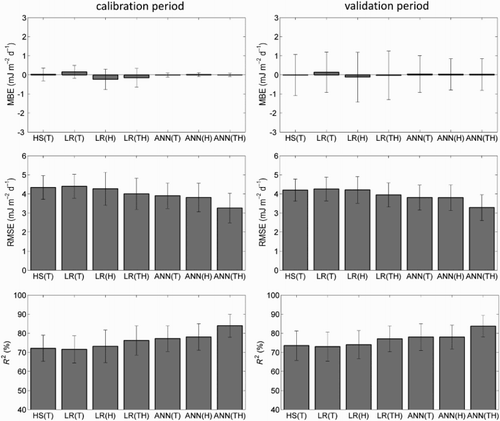
A typical problem of the ANN backpropagation algorithm is the possibility of ending up in a local minimum of the error function. However, the BRBP algorithm produces stable output with the RMSEs in the range of 0.01 to 0.02 MJ m⁻²d⁻¹, while minimizing both the squared error and the number of ANN model parameters to train.

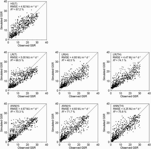
In Fig. 4, daily GSRs simulated by the seven models are compared with observations using scatterplots for the validation period at station 12. This station is selected for the following two main reasons: firstly, it successfully calibrates the stochastic models using a station with weaker correlations between GSR and predictors, which demonstrates the robustness of the approach; secondly, the predictors for station 12 have quite different statistical characteristics compared with the other stations (Table 2). However, the performances of the seven models at station 12 are generally consistent with the average performances of all stations provided in Fig. 4, and ANN(TH) yields the best agreement with the 1:1 line of the seven models.

Fig. 4 Scatterplots between observed and simulated daily GSR (MJ m⁻² d⁻¹) for the seven models at station 12 for the validation period.

b Regional Stochastic Models

Ordinary and universal kriging approaches are considered for spatial interpolation of the estimated coefficients of HS(T) and three linear regression models. The estimated coefficients of the HS(T) and LR(T) models display some spatial coherence based on the coordinates of the stations, but this is not the case for the LR(H) and LR(TH) models because of a weak spatial coherence of relative humidity (Fig. 2). The universal kriging approach is applied to the spatial interpolation of the estimated coefficients of HS(T) and LR(T) at 19 observation stations using the leave-one-out procedure. The evaluation of the interpolation performance is conducted by comparing the at-site estimated coefficients of the HS(T) and LR(T) models with the interpolated coefficients. Latitudes and longitudes of stations are employed as independent variables for the trend estimation of the universal kriging because the estimated coefficients of the two models are linearly correlated with the coordinates of the stations. As mentioned earlier, the coefficients of the regional LR(H) and LR(TH) models are estimated using a leave-one-out calibration procedure.

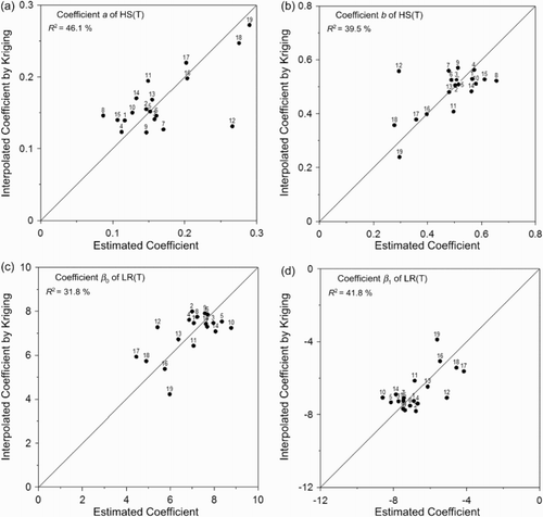
Figure 5 presents the scatterplots of the at-site estimated coefficients from observed data at each station and the interpolated coefficients from the universal kriging approach for the HS(T) and LR(T) models. In Figs 5a and 5b, the estimated coefficients and of the HS(T) model showed some spatial patterns. Coefficient increases with station latitude whereas coefficient decreases with latitude, particularly for stations 16 to 19, which are located in the middle or northern part of Quebec. The interpolated coefficients a and b show significant positive correlations with the at-site estimated coefficients with r² of 46.1 and 39.5%, respectively. Differences between interpolated and at-site estimated coefficients of station 12 are larger than those of the other stations because it is located at low altitude on the south shore of the Lower St. Lawrence valley, which has complex climate conditions resulting from the presence of a large river (St. Lawrence) and convection effects from continental and Atlantic Ocean air masses. In fact, a lower mean and standard deviation of DTR are observed at that station than at other stations (see Table 2). In Figs 5c and 5d, the estimated coefficients and of the LR(T) model also showed some spatial patterns. For instance, the estimates of the constant are small, whereas the estimates of slope of the temperature ratio are large for stations 12, 16, 17, 18, and 19 compared with the other stations. Kriging approaches cannot interpolate the regional coefficients of LR(H) and LR(TH) properly because spatial coherence between solar transmissivity and relative humidity are not as significant as those between solar transmissivity and the temperature ratio (see Table 2).

Fig. 5 Scatterplots between the at-site estimated coefficients of HS(T) and LR(T) and the interpolated coefficients using universal kriging and a leave-one-out procedure. Numbers represent stations shown in Table 1.

Table 3 presents RMSEs of the regional models for the 19 observation stations. The regional ANN(T) model performs better than the HS(T) and LR(T) for all stations except station 12. Moreover, regional HS(T) generally performs better than the regional LR(T). Although station 12 showed the largest difference between at-site estimated and interpolated coefficients for the HS(T) model (see Figs 5a and 5b), the regional HS(T) performs better than the regional ANN(T). Similarly, the regional HS(T) has, on average, an RMSE that is 0.19 MJ m⁻²d⁻¹ larger than the at-site HS(T) while the regional ANN(T) produces an RMSE that is 0.26 MJ m⁻²d⁻¹ larger than the at-site ANN(T). On average, the regional ANN(H) performs better than the regional LR(H). Again, the difference in RMSEs between regional and at-site ANN(H)s (0.34 MJ m⁻²d⁻¹) is larger than those between regional and at-site LR(H) (0.10 MJ m⁻²d⁻¹). A comparison of regional LR(TH) with ANN(TH) generally shows that ANN(TH) performs better than LR(TH). On average, the regional LR(TH) produces an RMSE that is 0.15 MJ m⁻²d⁻¹ larger than the at-site LR(TH). However, the difference in average RMSEs between regional and at-site ANN(TH)s is 0.43 MJ m⁻²d⁻¹. Therefore, it is obvious that the regional ANN-based models are more sensitive to new predictor values than the regional power function and linear regression models. Nonetheless, the three regional ANN models still perform better, on average, than the regional HS(T) and the three regional linear regression models for the same input variable.

Table 3. Comparison of RMSEs (MJ m⁻² d⁻¹) of the regional power function (i.e., HS(T)), linear regression (i.e., LR(T), LR(H), and LR(TH)), and non-linear ANN-based (i.e., ANN(T), ANN(H) and ANN(TH)) models for the validation period. The smallest RMSE is in bold for each station.

No.	Temperature			Relative Humidity		Temperature and Relative Humidity
	HS(T)	LR(T)	ANN(T)	LR(H)	ANN(H)	LR(TH)	ANN(TH)
1	4.18	4.30	3.92	4.42	4.21	4.05	3.61
2	4.48	4.28	4.03	4.28	3.96	3.85	3.43
3	4.15	4.33	3.77	4.15	3.93	3.86	3.34
4	4.05	4.27	4.01	4.08	4.14	3.76	3.40
5	4.60	4.93	4.32	4.38	4.16	4.00	3.43
6	3.70	3.70	3.36	3.61	3.27	3.35	2.97
7	4.14	4.27	3.83	3.86	3.68	3.45	3.08
8	4.96	5.44	4.58	4.02	3.82	4.07	3.60
9	4.15	4.43	3.77	4.27	4.14	3.76	3.36
10	4.52	4.96	4.25	4.39	4.27	4.00	3.69
11	4.22	4.34	3.96	3.85	3.64	3.63	3.32
12	5.21	5.51	5.31	5.24	5.48	5.12	5.38
13	4.53	4.37	4.14	4.06	4.36	3.80	3.79
14	4.08	4.90	3.91	4.65	4.30	4.29	4.27
15	4.00	4.16	3.87	5.30	5.21	4.49	4.45
16	4.13	4.19	3.99	3.65	3.56	3.44	3.27
17	4.68	4.54	3.87	3.98	4.16	3.88	4.10
18	4.37	3.88	3.26	3.62	4.16	3.49	3.54
19	5.04	4.85	4.81	4.88	4.64	5.31	4.72
Avg	4.38	4.51	4.05	4.25	4.16	3.98	3.72

In terms of input variables, the daily relative humidity explains the daily GSR as well as the temperature. The RMSE for the regional LR(H) is 0.13 MJ m⁻²d⁻¹ smaller than for the regional HS(T), whereas the RMSE for the regional ANN(H) is 0.10 MJ m⁻²d⁻¹ larger than for the regional ANN(T). By using both relative humidity and temperature, the RMSEs for the regional ANN(TH) are 0.33 and 0.44 MJ m⁻²d⁻¹ smaller than for the regional ANN(T) and ANN(H), respectively. Similarly, the RMSEs for the regional LR(TH) are 0.40 and 0.27 MJ m⁻²d⁻¹ smaller than for the regional HS(T) and LR(H), respectively.

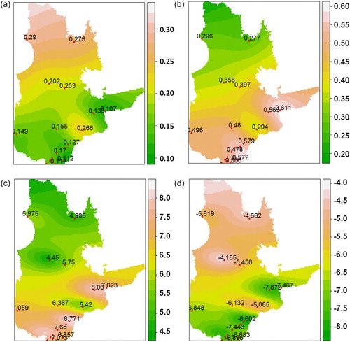
In Figs 6a–6d, interpolation maps of the HS(T) and LR(T) coefficients produced using universal kriging based on the estimated coefficients from all 19 stations are presented. In these figures, the coefficients generally increase or decrease with increasing latitude (°N to north) and longitude (°W to west) of the stations. Although, interpolation maps of both HS(T) and LR(T) are presented, the HS(T) model should be preferred to the LR(T) according to the regionalization performance presented in Table 3. Equations of the regional LR(H) and LR(TH) models using estimated coefficients from all the time series for all 19 stations at the 95% confidence level for these estimates based on an F-test are as follows:

Fig. 6 Interpolated maps of the regional HS(T) and LR(T) coefficients for the study area.

Regional LR(H):(13)

Regional LR(TH):(14)

Based on the expected performance levels presented in Table 3, the maps and equations are applicable to simulating daily GSR at a station that only measures daily maximum and minimum temperatures and/or relative humidity. For the study region, regional ANN models perform better than regional HS(T) and linear regression models; however, the latter are directly applicable without further development based on the maps and equations provided.

5 Discussion and conclusions

This study evaluates the separate and combined use of daily relative humidity and temperature as input variables to simulate daily GSR for the entire province of Quebec, Canada, as a complement to the univariate use of daily DTR to simulate daily GSR for a limited region in southern Quebec (Fortin et al., 2008). One power function, three linear regression, and three non-linear ANN-based models are developed at each of the selected 19 stations and their performances are evaluated. Of the seven models, ANN(TH), which uses daily maximum and minimum temperature and relative humidity as input variables, produced the best performance in terms of RMSE and r². The ANN-based models generally perform better than the other models with the same input variable conditions. This work is consistent with many previous studies (e.g., Benghanem et al., 2009; Fortin et al., 2008; Jiang, 2008; Mubiru & Banda, 2008; Tymvios et al., 2005) that reported the superiority of the ANN approach over other approaches as a transfer function. Therefore, ANN(T), ANN(H), and ANN(TH) are good tools for extending short records of daily GSR at a station according to the available temperature and/or relative humidity observations. Daily relative humidity provides as good a simulation of daily GSR as daily temperature in the study area. Furthermore, by using both temperature and relative humidity as input variables, the RMSEs for ANN(TH) are 0.50 and 0.53 MJ m⁻²d⁻¹ smaller than for ANN(T) and ANN(H), respectively, while the RMSEs for LR(TH) are 0.43 and 0.32 MJ m⁻²d⁻¹ smaller than for LR(T) and LR(H), respectively.

The regionalization ability of the power function, linear regression, and non-linear ANN-based models was evaluated. Interpolated coefficients of HS(T) and LR(T) using universal kriging are in good agreement with estimated coefficients from observed data at each station (see Figs 5a–5d and associated r²). However, the regional HS(T) model performs better than the regional LR(T) (see Table 3). A leave-one-out calibration procedure is used for the regional LR(H) and LR(TH) models because of the lack of spatial correlations among the estimated at-site coefficients. Regional ANN(T), ANN(H), and ANN(TH) models are also evaluated using a leave-one-out training procedure. On average, the regional ANN models perform better than the other regional models with the same input conditions (see Table 3) although the three regional ANN models are more sensitive to the new station dataset. This result partially supports the findings of Fortin et al. (2008) who applied the regional ANN(T) and HS(T) models to their study area (i.e., southern Quebec) and found that the former performed better than the latter. For our study area, interpolated coefficients of the regional HS(T) and LR(T) models and equations of the regional LR(H) and LR(TH) models are provided. These regional models may be preferable to regional ANN-based models because they can be used directly to simulate daily GSR at ungauged stations that measure daily temperature and relative humidity in Quebec, Canada, without further development.

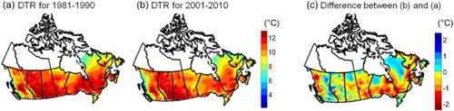
This study included four observation stations located in the middle of Quebec and in northern Quebec because it was initially intended to produce a directly applicable daily GSR dataset for modelling the salmonid thermal habitats over the entire province of Quebec (Bélanger et al., unpublished manuscript, 2015). Although the four stations are important to the assessment of the model regionalization approaches, the analysis periods of the four stations are different from the other stations because of data limitations (see Table 1). Consequently, the regional analysis might be affected by this difference in periods because the various calibration windows may lead to different relationships between the GSR and meteorological variables. For instance, gridded observations of daily T_max and T_min over Canada (see Hopkinson et al. (2011) and Jeong et al. (2015) for detailed descriptions) have generally similar spatial distributions of mean DTRs between the 1980s and 2000s (Figs 7a and 7b), particularly for this study area. However, they also yield some spatial differences of the anomaly between the two periods (Fig. 7c), but these differences are statistically insignificant according to the two-sample t-test with a 95% confidence level in all cases in the study area. This study employed a leave-one-out procedure to test regional models; however, additional cross-validation procedures could be considered in future work to test the robustness of the regional models instead of validating on one section of the data.

Fig. 7 Mean values of DTRs for the (a) 1981–1990 and (b) 2001–2010 periods over Canada. Differences between (b) and (a) are presented in (c). Gridded observations of daily T_max and T_min (Hopkinson et al., 2011; Jeong et al., 2015) are used for this assessment.

Acknowledgements

We would like to thank David Huard from Ouranos for his help.

Disclosure statement

No potential conflict of interest was reported by the authors.

Additional information

Funding

This study was financed by a team grant from Ouranos to Yves Gratton, André St-Hilaire, Isabelle Laurion, and J.-C Auclair and by NSERC Discovery grants to André St-Hilaire, Isabelle Laurion, and Yves Gratton.

References

- Abraha, M. G., & Savage, M. G. (2008). Comparison of estimates of daily solar radiation from air tempreature range for application in crop simulations. Agricultural and Forest Meteorology, 148, 401–416. doi:10.1016/j.agrformet.2007.10.001
- Behrang, M. A., Assareh, E., Noghrehabadi, A. R., & Ghanbarzadeh, A. (2011). New sunshine-based models for predicting global solar radiation using PSO (particle swarm optimization) technique. Energy, 36(5), 3036–3049. doi:10.1016/j.energy.2011.02.048
- Bélanger, C., Huard, D., Gratton, Y., Jeong, D. I., St-Hilaire, A., Auclair, J. C., & Laurion, I. (2013). Impacts des changements climatiques sur l'habitat des salmonidés dans les lacs nordiques du Québec. Rapport INRS – Eau, Terre, Environnement pour Ouranos. Québec, Canada: INRS-ETE.
- Benghanem, M., Mellit, A., & Alamri, S. N. (2009). ANN-based modelling and estimation of daily global solar radiation data: A case study. Energy Conversion and Management, 50(7), 1644–1655. doi:10.1016/j.enconman.2009.03.035
- Bristow, K. L., & Campbell, G. S. (1984). On the relationship between incoming solar radiation and daily maximum and minimum temperature. Agricultural and Forest Meteorology, 31, 159–166. doi:10.1016/0168-1923(84)90017-0
- Cutforth, H. W., & Judiesch, D. (2007). Long-term changes to incoming solar energy on the Canadian Prairie. Agricultural and Forest Meteorology, 145(3–4), 167–175. doi:10.1016/j.agrformet.2007.04.011
- De Jong, R., & Stewart, D. W. (1993). Estimating global solar radiation from common meteorological observations in western Canada. Canadian Journal of Plant Science, 73(2), 509–518. doi: 10.4141/cjps93-068
- De La Casiniere, A., Bokoye, A. I., & Cabot, T. (1997). Direct solar spectral irradiance measurements and updated simple transmittance models. Journal of Applied Meteorology, 36(5), 509–520. doi: 10.1175/1520-0450(1997)036<0509:DSSIMA>2.0.CO;2
- Ertekin, C., & Evrendilek, F. (2007). Spatio-temporal modeling of global solar radiation dynamics as a function of sunshine duration for Turkey. Agricultural and Forest Meteorology, 145, 36–47. doi:10.1016/j.agrformet.2007.04.004
- Fletcher, D., & Goss, E. (1993). Forecasting with neural networks: An application using bankruptcy data. Information and Management, 24, 159–167. doi:10.1016/0378-7206(93)90064-Z
- Fortin, J. G., Anctil, F., Parent, L. E., & Bolinder, M. A. (2008). Comparison of empirical daily surface incoming solar radiation models. Agricultural and Forest Meteorology, 148(8–9), 1332–1340. doi:10.1016/j.agrformet.2008.03.012
- Goovaerts, P. (1997). Geostatistics for natural resources evaluation. New York, USA: Oxford University Press.
- Gueymard, C. (1989). A two-band model for the calculation of clear sky solar irradiance, illuminance and photosynthetically active radiation at the earth's surface. Solar Energy, 43, 253–265. doi:10.1016/0038-092X(89)90113-8
- Gul, M. S., Muneer, T., & Kambezidis, H. D. (1998). Models for obtaining solar radiation from other meteorological data. Solar Energy, 64(1), 99–108. doi:10.1016/S0038-092X(98)00048-6
- Hargreaves, G. H., & Samani, Z. A. (1982). Estimating potential evapotranspiration. Journal of Irrigation and Drainage Engineering, 108, 225–230.
- Haykin, S. (1994). Neural networks. New York, USA: MacMillan College Publishing Company.
- Hopkinson, R. F., McKenney, D. W., Milewska, E. J., Hutchinson, M. F., Papadopol, P., & Vincent, L. A. (2011). Impact of aligning climatological day on gridding daily maximum-minimum temperature and precipitation over Canada. Journal of Applied Meteorology and Climatology, 50(8), 1654–1665. doi:10.1175/2011JAMC2684.1
- Hunt, L. A., Kuchar, L., & Swanton, C. J. (1998). Estimation of solar radiation for use in crop modelling. Agricultural and Forest Meteorology, 91, 293–300. doi:10.1016/S0168-1923(98)00055-0
- Hussain, M., Rahman, L., & Rahman, M. R. (1999). Techniques to obtain improved predictions of global radiation from sunshine duration. Renewable Energy, 18(2), 263–275. doi:10.1016/S0960-1481(98)00772-1
- Isaaks, E. H., & Srivastava, R. M. (1989). An introduction to applied geostatistics. New York, USA: Oxford University Press.
- Jackson, L. S., & Forster, P. M. (2010). An empirical study of geographic and seasonal variations in diurnal temperature range. Journal of Climate, 23(12), 3205–3221. doi:10.1175/2010JCLI3215.1
- Jeong, D. I., Sushama, L., Diro, G. T., Khaliq, M. N., Beltrami, H., & Caya, D. (2015). Projected changes to high temperature events for Canada based on a regional climate model ensemble. Climate Dynamics, Advance online publication. doi:10.1007/s00382-015-2759-y
- Jiang, Y. (2008). Prediction of monthly mean daily diffuse solar radiation using artificial neural networks and comparison with other empirical models. Energy Policy, 36(10), 3833–3837. doi:10.1016/j.enpol.2008.06.030
- Leckner, D. (1978). The spectral distribution of solar radiation at the earth's surface-elements of a model. Solar Energy, 20, 143–150. doi:10.1016/0038-092X(78)90187-1
- Liu, X., Mei, X., Li, Y., Wang, Q., Jensen, J. R., Zhang, Y., & Porter, J. R. (2009). Evaluation of temperature-based global solar radiation models in China. Agricultural and Forest Meteorology, 149, 1433–1446. doi:10.1016/j.agrformet.2009.03.012
- Mahmood, R., & Hubbard, K. G. (2002). Effect of time of temperature observation and estimation of daily solar radiation for the northern Great Plains, USA. Agronomy Journal, 94(4), 723–733. doi:10.2134/agronj2002.7230
- Miller, D. G., Rivington, M., Matthews, K. B., Buchan, K., & Bellocchi, G. (2008). Testing the spatial applicability of the Johnson-Woodward method for estimationg solar radiation from sunshine duration data. Agricultural and Forest Meteorology, 148, 466–480. doi:10.1016/j.agrformet.2007.10.008
- Mubiru, J., & Banda, E. J. K. B. (2008). Estimation of monthly average daily global solar irradiation using artificial neural networks. Solar Energy, 82(2), 181–187. doi:10.1016/j.solener.2007.06.003
- Nimnuan, P., & Janjai, S. (2012). An approach for estimating average daily global solar radiation from cloud cover in Thailand. Procedia Engineering, 32, 399–406. doi:10.1016/j.proeng.2012.01.1285
- Podestá, G. P., Núñez, L., Villanueva, C. A., & Skansi M. A. (2004). Estimating daily solar radiation in the Argentine Pampas. Agricultural and Forest Meteorology, 123, 41–53. doi:10.1016/j.agrformet.2003.11.002
- Rivington, M., Bellocchi, G., Matthews, K. B., & Buchan, K. (2005). Evaluation of three model estimations of solar radiation at 24 UK stations. Agricultural and Forest Meteorology, 132, 228–243. doi:10.1016/j.agrformet.2005.07.013
- Sellers, W. K. (1965). Physical climatology. Chicago: University of Chicago Press.
- Trnka, M., Žalud, Z., Eitzinger, J., & Dubrovský, M. (2005). Global solar radiation in Central European lowlands estimated by various emprical formulae. Agricultural and Forest Meteorology, 131, 54–76. doi:10.1016/j.agrformet.2005.05.002
- Tymvios, F. S., Jacovides, C. P., Michaelides, S. C., & Scouteli, C. (2005). Comparative study of Ångström's and artificial neural networks’ methodologies in estimating global solar radiation. Solar Energy, 78(6), 752–762. doi:10.1016/j.solener.2004.09.007
- Weiss, A., & Hays, C. (2004). Simulation of daily solar irradiance. Agricultural and Forest Meteorology, 123, 187–199. doi:10.1016/j.agrformet.2003.12.002