Decadal Trends in Oxygen Concentration in Subsurface Waters of the Northeast Pacific Ocean

Abstract

Previous studies have shown decreasing oxygen concentration (O₂) in subsurface waters of the continental slope from California to Canada since about 1980. With longer time series we show that from southern California to northern Canada increasing O₂ preceded these decreases from 1950 to about 1980. Because there has been no clear trend since 1950, we cannot yet conclude that anthropogenic climate change is the cause of these decreasing trends after 1980. These findings are based mainly on O₂ on the 26.7 potential density (σ_θ) surface in the region north of 30°N and east of 170°W, covering both the continental margin and deep-sea regions. On the continental slope, O₂ increased at most locations by 10 to 20 µmol kg⁻¹ to about 1980, followed by declines of similar magnitude in recent years. Changes in O₂ were associated with changes in temperature of the opposite sign south of 37°N, but correlation of temperature and O₂ is irregular in more northerly locations. At all locations, temperature-related solubility change was a minor cause of these O₂ trends. In deep-sea waters, O₂ decreased with time with a more rapid decrease from about 1995 to about 2003. At Ocean Station P (OSP; 50°N, 145°W), which has the longest uninterrupted record of observations, significant linear trends of −0.4 to −0.5 µmol kg⁻¹y⁻¹ were found on the 26.5, 26.7, and 26.9 σ_θ surfaces. In addition, a significant sinusoidal oscillation of period 18.61 years and amplitude of 18 µmol kg⁻¹ was found on the 26.9 σ_θ surface at OSP and a station 400 km to the east, which fits reasonably well with the lunar nodal cycle. The phase of this oscillation was identical at both locations. Clear evidence of similar variability did not emerge at other open-ocean locations or along the continental slope.

RÉSUMÉ

[Traduit par la rédaction] Des études antérieures ont montré que la concentration en oxygène (O₂) a diminué dans les eaux de subsurface de la pente continentale, de la Californie jusqu'au Canada, et ce, depuis environ 1980. À l'aide de longues séries temporelles, nous montrons qu'une augmentation de la quantité d'O₂ a précédé ces diminutions, entre 1950 et environ 1980, du sud de la Californie jusque dans le nord du Canada. Comme il n'existe pas de tendance évidente depuis 1950, nous ne pouvons conclure que des changements climatiques d'origine humaine causent ces tendances à la baisse après 1980. Nous fondons surtout ces conclusions sur la concentration d'O₂ au niveau de densité potentielle (σ_θ) de 26,7 qui couvre la région au nord de 30° N et à l'est de 170° O, comprenant à la fois la marge continentale et la haute-mer. Sur la pente continentale, la quantité d'O₂ a augmenté de 10 à 20 µmol kg⁻¹ à la plupart des emplacements jusqu'en 1980. Ces dernières années, elle a diminué du même ordre de grandeur. Ces modifications des concentrations d'O₂ étaient associées à des changements de température de signe opposé, au sud de 37° N, mais la corrélation entre la température et la quantité d'O₂ est irrégulière pour les endroits les plus au nord. À tous les emplacements, le changement de solubilité lié à la température restait une cause mineure des tendances de l'O₂. En haute-mer, le taux d'O₂ a diminué avec le temps. Ce déclin s'est accentué entre environ 1995 et 2003. À la station océanique P (50° N, 145° O), qui possède la plus longue série ininterrompue d'observations, nous avons calculé des tendances linéaires significatives de −0,4 à −0,5 µmol kg⁻¹ a⁻¹, aux surfaces de σ_θ égales à 26,5, 26,7 et 26,9. Nous avons aussi détecté une oscillation sinusoïdale significative d'une période de 18,61 années et d'une amplitude de 18 µmol kg⁻¹ au niveau de σ_θ égale à 26,9, à la station P et à une station située 400 km plus à l'est. Ces résultats correspondent raisonnablement bien avec le cycle des nœuds lunaires. La phase de cette oscillation était identique aux deux sites. L’évidence nette d'une telle variabilité n'est pas ressortie à d'autres sites hauturiers ni le long de la pente continentale.

KEYWORDS:

• climate change ocean
• oxygen concentration
• decadal variability
• continental margin
• northeast Pacific Ocean

1 Introduction

Subsurface waters of the continental slope off the west coast of the Americas are chronically low in oxygen (O₂). Whereas ocean surface waters everywhere are usually saturated with O₂, with a concentration close to 300 μmol kg⁻¹, O₂ declines rapidly with increasing depth below the ocean surface mixed layer. The rate of decline with depth is significantly greater along the west coast of the Americas than is typical of the ocean in general, as seen in the concentration of O₂ on the 26.75 neutral density surface in the Pacific Ocean (Fig. 1).

Fig. 1 Oxygen concentration (O₂; μmol kg⁻¹) on the 26.75 neutral density surface in the Pacific Ocean. A neutral density is a seawater potential density whose reference surface varies continuously with pressure (Ivers, 1975; Jackett & McDougall, 1997). The depth of this neutral density surface ranges from near zero in the northwest Pacific Ocean and zero in the Southern Ocean to about 300 m off Central America. Figure from WOCE Pacific Ocean Atlas by permission (Talley, 2007; http://www-pord.ucsd.edu/whp_atlas/pacific_index.html).

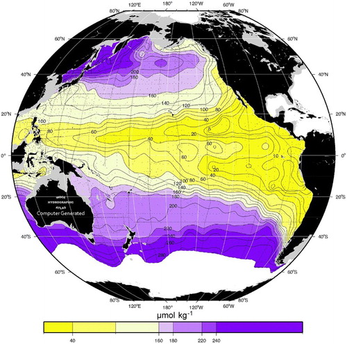
The concentration of O₂ is highest in the northwest Pacific Ocean and in the Southern Ocean where this neutral density surface outcrops but declines towards the east between 40° and 60°N in the general flow direction of North Pacific Intermediate Water. Low O₂ along the eastern side of the Pacific Ocean is attributed to the increased age of subsurface waters and also to enhanced oxidation rates associated with high primary productivity resulting from coastal upwelling of nutrient-rich waters. In general, O₂ below the surface mixed layer declines throughout the ocean in the direction of flowing subsurface ocean currents because of oxidation of organic detritus. However, O₂ increases towards the north along the west coast of North America in the direction of flow of the California Undercurrent (CUC) that carries Pacific Equatorial Water from regions west of Central America. This opposite spatial gradient in the CUC is attributed to mixing with more oxygenated offshore waters (Meinvielle & Johnson, 2013; Pelland, Eriksen, & Lee, 2013; Thomson & Krassovski, 2010).

a Continental Slope

Several studies have found declining O₂ along the North American continental shelf and slope in the past few decades. Whitney, Freeland, and Robert (2007) noted that O₂ declined by 1.22 μmol kg⁻¹y⁻¹ from 1987 to 2006 at station P4 on the continental slope west of Vancouver Island. Chan et al. (2008) and Service (2004) described observations of O₂ less than 0.5 ml L⁻¹ (1 ml L⁻¹ ≈ 43 μmol kg⁻¹) in subsurface waters on the Oregon continental shelf during several summers beginning in 2002, a condition not observed between 1950 and 1999. Bograd et al. (2008, 2015) found declines in subsurface O₂ off southern California from 1984 to 2012. Whitney (2009) found a decline in O₂ west of Haida Gwaii (formerly the Queen Charlotte Islands) from about 1982 to 2007. Pierce, Barth, Shearman, and Erofeev (2012) describe a decrease in O₂ on the Oregon shelf and slope while comparing observations from 1960 to 1971 with those from 1998 to 2009. Crawford and Peña (2013) note declines in subsurface O₂ on the Vancouver Island shelf and slope based on observations from 1979 to 2001. Meinvielle and Johnson (2013) found decreasing subsurface O₂ all along the continental shelf break between 25° and 50°N for the period from 1980 to 2012, with the greatest trend being near the core of the CUC. This trend is accompanied by warmer and saltier waters on individual density surfaces in the CUC, as well as decreasing potential vorticity.

Only a few studies analyze trends in O₂ from the 1950s to the 1980s, and these are mostly confined to Central America or the southern California region covered by the California Cooperative Fisheries Investigation (CalCOFI). McClatchie, Goericke, Cosgrove, Auad, and Vetter (2010) examine O₂ concentration on the 26.6 potential density (σ_θ) surface at stations in the California Bight and its offshore boundary. Their study reveals that O₂ increased by 0.15 ml L⁻¹ between 1950 and 1990 and decreased by 0.3 ml L⁻¹ from 1990 to 2007. Koslow, Goericke, Lara-Lopez, and Watson (2011) examined mean O₂ between 200 and 400 m depth at 51 CalCOFI stations that were consistently sampled from 1951 to 2008 and that extended from San Diego to north of Point Conception, California, and from the coast (∼50 m depth) to about 400 km offshore. Their results reveal several peaks in O₂ concentration between 1972 and 1998, preceded and followed by much lower O₂ in the 1950s and 2000s. The peaks are about 0.5 ml L⁻¹ higher than O₂ at the beginning and end of the period. A similar pattern of variability is noted by Deutsch, Brix, Ito, Frenzel, and Thompson (2011) off Central America. Meinvielle and Johnson (2013, their Fig. 1b) show visual evidence of increasing O₂ from 1950 to about 1980 on the 26.5 σ _θ surface at 35°N in waters of depth 800 m but do not discuss measurements prior to 1980 elsewhere in their paper. These studies reveal a need to examine observations all along the US and Canadian continental margin from at least the 1950s to determine whether this maximum in O₂ is found at more northern latitudes.

A comparison of decadal variability along the continental margin could provide insight into the causes of variability. Off Central America, Deutsch et al. (2011) attribute the decadal variability of subsurface O₂ to links between local upwelling winds and oxidation of detritus. Changes in local winds determine the rate of upwelling of nutrients into the upper layer, which leads to changes in phytoplankton productivity and in organic detritus sinking through subsurface layers, leading to changes in O₂ utilization and concentration. These subsurface, modified Pacific Equatorial Water flow northward in the CUC along the continental slope all the way to Alaska (Thomson & Krassovski, 2010), so water masses all along the North American margin share a common source, and possibly a common decadal variability, because of advection. Meinvielle and Johnson (2013) suggest that increased amounts of Pacific Equatorial Water have been transported northward since 1980, carrying more water low in O₂ northward. In addition, the subsurface waters at the southern limit of their domain (25°N) have experienced lower O₂ since 1980, further reducing the O₂ available for northward transport. However, as mentioned earlier, the CUC is strongly diluted by mixing with offshore, more oxygenated water (Pelland et al., 2013), and the path of the CUC from Central America to southern Canada lies in a region of strong coastal upwelling and productivity accompanied by sinking detritus and local subsurface oxidation. Any local change in mixing and upwelling could also lead to decadal variability in O₂.

b Deep-Sea

Studies of decadal changes in O₂ in deep-sea waters of the Northeast Pacific have focused mainly on Ocean Station P (OSP) at 50°N, 145°W. Regular sampling of O₂ has taken place at OSP since 1956 and the time series of these measurements is one of the most complete in any deep-sea region. These studies (Andreev & Baturina, 2006; Cummins & Masson, 2012; Falkowski et al., 2011; Whitney et al., 2007) note a general decline in O₂ in the thermocline and halocline since 1956. Cummins and Masson (2012) note that O₂ changes resulting from vertical heaving of constant density surfaces are dominant at 150 and 200 m depth and are comparable to O₂ changes on constant density surfaces at 250 m. On the other hand, because of the smaller vertical gradient, low-frequency O₂ variability at greater depths is driven mainly by variations occurring on isopycnals. In both the east and west North Pacific subarctic gyres, Watanabe, Shigemitsu, and Tadokoro (2008) found a decrease of O₂ of 0.74 μmol kg⁻¹ per year on the 26.8 σ _θ surface based on observations beginning in 1968 and 1956 in the western and eastern gyres, respectively. All eastern gyre observations are at OSP.

Three of the Line P studies note decadal variability of O₂ on constant density surfaces at OSP that fits reasonably well with the 18.6-year lunar nodal cycle (LNC). Similar oscillations have been observed in the western North Pacific, so changes in O₂ at OSP could be linked to decadal variability in O₂ in the Northwest Pacific or Aleutians (Andreev & Baturina, 2006), where significant LNC variability on subsurface O₂ on constant density surfaces has been traced from the outflow of the Sea of Okhotsk into the western and central North Pacific Ocean (Osafune, Masuda, & Sugiura, 2014; Osafune & Yasuda, 2013; Yasuda, Osafune, & Tatebe, 2006). Variability in the LNC arises from the 18.6-year cycle of the declination of the lunar orbit, which in turn modulates diurnal tidal amplitudes by as much as 20%. It is believed that variations in tidal mixing due to the varying tidal amplitude create variability in the density and O₂ content of waters flowing through the Kuril Islands between the Sea of Okhotsk and the North Pacific Ocean. Because this flow is a component of the North Pacific Intermediate Water, variations in O₂ of the LNC period are suspected to propagate eastward across the North Pacific Ocean, reaching OSP from Japan in about six to seven years (Keeling, Körtzinger, & Gruber, 2010; Whitney et al., 2007).

Several studies report O₂ concentration in units of apparent oxygen utilization (AOU), where AOU is the difference between saturation and measured O₂. If variations in the saturation of O₂ are small when AOU variations are examined along constant density surfaces, then changes in AOU are about equivalent to O₂ changes of equal size but opposite in sign. In the Northeast Pacific Ocean, Emerson, Watanabe, Ono, and Mecking (2004) described the changes in O₂, temperature, and salinity in great detail for the years 1980 to 2000, focusing on repeat tracks along 47°N, 152°W and 165°E. They found an increase in AOU in the pycnocline below the mixed layer all across the North Pacific. Along 152°W, they note that AOU in the pycnocline increased from 1984 to 1997, with the greatest increase of 28.6 μmol kg⁻¹ on the constant density layer between 26.2 and 26.4. At 26.6 to 26.8, the increase in AOU was 8.7 μmol kg⁻¹. Mecking et al. (2008) showed comparisons of AOU along 152°W decade-by-decade. They found a significant increase in AOU from the 1980s to 2006 at most latitudes between 27° and 56°N, with the smallest increase occurring in the latitude range 47° to 50°N. To the north of 38°N the most significant increase in AOU occurred from 1991 to 1997. These previous studies did not compare deep-sea and continental margin observations of O₂ on σ _θ surfaces over the full archived set of data.

c Objectives

In this study, we present decadal trends of O₂ concentration on σ_θ surfaces below the ocean surface mixed layer, along the west coast of North America from California to northern Canada and in deep-sea waters north of 30°N and east of 170°W. The data search includes all archived observations since the 1930s, to examine decadal changes in O₂ over as many decades as possible, hoping this larger dataset will provide insight into overarching temporal variability. A more specific goal is to determine whether the increase in O₂ observed off southern California prior to the 1980s is also present along the continental slope farther north and whether it extends into deep-sea waters. We include temperature observations in our analyses to allow interpretation of causes of O₂ variability and of linkages of trends in O₂ among regions.

2 Data

a Data Preparation

Water property data were retrieved from the archives of the US National Ocean Data Center (NODC) and also from the archives of the Institute of Ocean Sciences, Fisheries and Oceans Canada, in Sidney, British Columbia, Canada. The geographical range selected was the Pacific Ocean north of 30°N and east of 170°W. Only samples that included O₂, temperature, and salinity were retrieved. Many profiles measure depth of samples by stating the water pressure, in which case pressure units were converted to depth in metres. At the time of downloading from NODC there were no samples after 2008. More recent data used in this paper are from the Fisheries and Oceans Canada archive. Only data with the highest quality flags were used in the analysis, and after careful examination of the data, it was necessary to remove only a few obvious outliers. Almost all observations were made on ocean research cruises, with O₂ measured by the Winkler titration method, or in recent years by regularly calibrated electronic sensors. Various units of O₂ concentration were converted to micromoles per kilogram (μmol kg⁻¹).

McClatchie et al. (2010) describe the expected errors in O₂ concentration measured by CalCOFI since 1950 and also the effect of the change in 1984 to automated end-point determination of the titration. They note that temporal changes are at least a factor of ten greater than any differences in precision between the early and late years of the CalCOFI time series. Whitney et al. (2007) note that the Winkler method has been used for OSP and Line P observations from the beginning, and although individual operators might produce slightly different O₂ concentrations, mainly due to end-point determination, the expected errors are small compared with decadal changes in O₂.

Salinity and temperature units were converted to Absolute Salinity (S_A; grams per kilogram), which is an SI unit of concentration, and Conservative Temperature (Θ), using formulae provided by the Thermodynamic Equation of Seawater–2010 (TEOS-10; www.teos-10.org/), which is based on a Gibbs function formulation from which all thermodynamic properties of seawater (σ _θ, enthalpy, entropy sound speed, etc.) can be derived in a thermodynamically consistent manner. The Intergovernmental Oceanographic Commission adopted TEOS-10 at its 25th Assembly in June 2009 to replace EOS-80 as the official description of seawater and ice properties in marine science. The TEOS-10 replacement for potential temperature is Θ, which is derived from potential enthalpy, an ideal conservative variable for heat content. The thermodynamic properties of seawater, such as σ _θ and enthalpy, are now correctly expressed in scientific literature as functions of S_A rather than being functions of the conductivity of seawater for practical salinity. The units of σ _θ are kilograms per cubic metre, and we identify density surfaces with the symbol σ _θ, which is the potential density anomaly and has the same units as potential density (kilograms per cubic metre) but differs in that 1000 kg m⁻³ have been subtracted.

We focus on O₂ on a constant σ _θ surface rather than at a constant depth, to reduce the impact of seasonal upwelling of deep water and to enable comparison of trends among widely separated regions of the Northeast Pacific Ocean. To determine O₂ on σ _θ surfaces, profiles sampled with hydro-bottles at discrete depths were linearly interpolated with one-metre vertical resolution. No interpolation was applied if any of O₂, Θ, or S_A were spaced more than 0.2 σ _θ units apart. The selection of O₂ was made from the interpolated, one-metre-resolution profiles only if σ _θ was within 0.005 of the specified density anomaly. The depth of the ocean bottom for each profile was read from the metadata accompanying each profile, if not provided it was computed from the latitude and longitude in the metadata, based on the Earth Topography 2-arc-min (ETOP02) database (Smith & Sandwell, 1997). Previous literature applies both sigma-theta (σ _θ) and sigma-t (σ_t) to this topic, but the depth difference between these surfaces is minor, reaching only a few metres at 300 m depth, and we opted to use σ _θ. The σ _θ surfaces that we apply in this paper are referenced to the ocean surface and are essentially the same as neutral density for the depths we consider.

We focus mainly on spatial and temporal trends on the 26.7 σ _θ surface because it is near the core of the CUC (Thomson & Krassovski, 2010) and is the least dense σ _θ surface that does not outcrop in the Northeast Pacific Ocean (Emerson et al., 2004; Mecking et al., 2008). In addition, it is very close to the central density of 26.8 of North Pacific Intermediate Water that is produced in the western North Pacific subpolar region (Talley, 1993) and the 26.5 σ _θ surface identified by Meinvielle and Johnson (2013) as the core of the CUC, based on maximum spiciness. Its depth below the layer of significant mixing with the ocean surface in the Northeast Pacific removes local O₂ injection from the atmosphere as a source of O₂ change. Reducing the factors that alter O₂ reduces the complexity of the interpretation of O₂ changes in time and space. Some trends on other σ _θ surfaces are also presented to indicate the degree of robustness of results and to examine O₂ changes at shallower depths where waters are likely to advect onto the adjacent continental shelf. Over most of the Northeast Pacific the 26.7 σ _θ surface lies below 200 m depth and thus beyond the continental shelf. Along the continental slope its depth shoals by 50 to 100 m from southern California to northern British Columbia.

b Regional Sampling

After merging databases and discarding duplicates, there were about 25,000 samples on each σ _θ surface. Most samples lie on the continental slope, with the greatest concentration off southern California in the region sampled by CalCOFI and from northern Oregon to British Columbia. Although 25,000 samples seems to be a great number, there are very few individual stations with samples in all decades since the 1940s. Almost all lie in the CalCOFI region of southern California. Seven CalCOFI stations were selected for trend analysis based on their locations along and across the axis of the CUC.

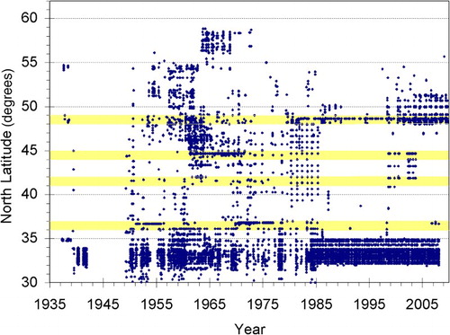
To the north of the CalCOFI region (above 35°N) there have been many sampling programs over the past decades, with observations collected over many different locations instead of at fixed stations. In this region we selected observations in four latitude bands on the continental slope where the bottom depth is between 210 and 1500 m, each with a north–south range of one degree of latitude. The shallow limit was chosen to remove samples from the continental shelf where water on a σ _θ surface might be present only during the upwelling season, when considerable within-season O₂ decreases might be due to oxidation of organic matter near the sea bottom (Adams, Barth, & Chan, 2013). The deep limit was chosen to enable us to confine our search to the continental slope and not extend it into deep-sea waters. Figure 2 presents a latitude-versus-year Hovmöller graph of O₂ measurements on the continental slope where the water depth is between 210 and 1500 m. This primary search region includes most of the CUC. The CUC is concentrated over the upper continental slope with the strongest flow at depths of 100–300 m (but some flow to at least 1000 m), a cross-shore scale of 10–50 km, peak speeds about 30–50 cm s⁻¹ and a volume transport of the order of 1 Sv (1 Sv = 10⁶m³s⁻¹) (Gay & Chereskin, 2009) based on many studies from Reid (1962) to Pierce, Smith, Kosro, Barth, and Wilson (2000). A final region was selected west of northern Canada from 51°–55°N, including shelf, slope, and deep-sea waters because few slope samples were available. Upwelling here is weak and its impact on O₂ near bottom on the continental shelf is minor.

Fig. 2 Hovmöller graph of O₂ sample locations on the 26.7 σ_θ surface of the continental slope where the bottom depth is between 210 and 1500 m. Regions shaded yellow denote latitude bands selected to examine trends in O₂ on the continental slope from 36° to 49°N.

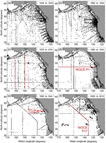
The open-ocean waters of the Northeast Pacific Ocean have been well sampled since the late 1940s, with regular sampling at OSP since 1956. However, apart from OSP there are no long-term stations available for examination, as shown in the plot of decade-by-decade distribution of observations (Fig. 3) since 1949. (Earlier measurements are mostly pre-World War II and sparse.) The measurements from 1949 to 1959 (Fig. 3a) are scattered across the region. The CalCOFI stations can be seen, along with regular lines of cross-slope stations to the north of the CalCOFI region. Through the decades until the 1990s the stations increasingly lie along single tracks. Unfortunately, none of these tracks repeat in every decade. In the most recent era (2000 to 2011; Fig 3f), observations by Argo floats are distinguished by their irregular and closely spaced distributions. Although Argo data locations are plotted in Fig. 3f, their observations were not used in our analyses of O₂ variability because the accuracy of their O₂ measurements is not better than plus or minus 3% (Emerson & Bushinsky, 2014; Takeshita et al., 2013) and their distribution in space and time seldom aligned with our selected locations and data gaps. Observations selected for open-ocean study are limited to regions with repeated sections in several decades, as well as stations along Line P including OSP, as indicated in Fig. 3e.

Fig. 3 Spatial distribution of O₂ samples interpolated onto the 26.7 σ_θ surface in the Northeast Pacific Ocean, by decade. Red lines show locations of deep-sea sections and lines discussed: (c) 149.5°–161.5°W; (d) WOCE line P1 along 47°N; (e) Line P with stations P8, P12, P16, P20, and OSP each marked with a red asterisk, progressing from east to west; (f) section along northern end of WOCE line P17.

c Statistical Test of Temporal Trends

For O₂ along the continental margin, statistical confidence in various polynomial least-squares regressions, from linear to cubic, was computed as follows. First, the seasonal cycle was examined by computing bimonthly averages of each time series. There is an observable seasonal cycle in O₂ on individual density surfaces at most locations, but its impact on decadal trends is minor because sampling is generally well distributed throughout the seasons over the time series, except at 41°–42°N where the seasonal distribution of sampling did vary from one decade to another. Nevertheless, an average annual cycle was removed from the observations (except at 41°–42°N) before statistical confidence in decadal trends was computed.

Then, an appropriate set of annual mean values of O₂ concentration was calculated for each location. This presented a challenge because sampling was unbalanced among years. Years with frequent sampling will have a well-determined annual mean, whereas years with little sampling will not. To retain the influence of greater or lesser uncertainty among years, a Monte Carlo resampling approach was adopted. The first step was to compute annual 95% confidence intervals (CI) for all years with three or more measurements, computed as ±1.996 times the standard error of the sample. The lower CI is at p = 0.025, and the upper CI is p = 0.975 for a two-tailed test with alpha equal to 0.05. This provides an annual “interval” estimate of central tendency of the data within a year rather than a “point” estimate, such as the annual mean.

Each Monte Carlo trial selected a random annual-mean O₂ concentration from within the lower and upper CI. Each time series was fit first to a linear model, then to a quadratic model, and finally to a cubic model, and the values of the estimated coefficients of interest were retained for each model. The total number of trials (fitting data to each of the three models) was 10,000. The main result of the trials was the frequency distribution for each coefficient. Using the linear model as an example, where the coefficient of interest is the slope, if the 95% CI on the slope, generated from the 10,000 trials, excluded zero, the null hypothesis of slope equal to 0.0 could be rejected. The same principle holds for the quadratic and cubic coefficients. Furthermore, it is possible for a time series to exhibit multiple patterns. For example, significant linear and quadratic terms might suggest a dome-shaped time series, with one end of the dome significantly higher, or lower depending on the sign, than the start of the series. A coefficient was considered to be significant at the 95% CI if it had the same sign in 95% of the trials. Quadratic polynomials fell within the 95% CI for more time series than did cubic polynomials. Thus, only the quadratic case (a + bx + cx²) is presented.

Along Line P we applied the commercial package SYSTAT, version 9, to annual means of O₂ observations, searching for significant linear and quadratic trends plus 18.6-year oscillations. This analysis is more suitable than the Monte Carlo type of search for statistical confidence applied to the continental margin because it is difficult to assess the number of degrees of freedom in each annual average in these Line P series, a critical input to the Monte Carlo approach. Because in many cases neighbouring observations at OSP and other Line P stations are for the same day but separated by 10 to 100 km, or at the same location on closely spaced days, there is no objective way to determine which observations are statistically independent from each other when computing confidence limits of each annual average.

3 Results and discussion

a Continental Slope

Observations of O₂ and its best fit quadratic polynomial to the annual average of O₂ with significant doming in time at the 95% CI (hereafter significant quadratic polynomial) are presented for locations along the continental slope from 32° to 49°N and on the shelf to deep-sea waters from 51° to 55°N. For Θ and the depth of the σ_θ surface, scatterplots and best-fit quadratic polynomials to all observations (hereafter trend lines) are presented because statistical tests of their temporal trends were not computed. Every observation is displayed in the various graphs to assess the decadal variability compared with other variability and short-term scattering and to evaluate qualitatively any gaps in the observations. Results for the 26.7 σ _θ surface are presented first, followed by supporting information for three other σ _θ surfaces.

1 Southern California (CalCOFI)

The CalCOFI program provides the most complete and spatially detailed set of observations along the west coast of North America. A set of stations was selected (Fig. 4) to analyze decadal trends on a section across the continental slope (stations 59, 63, 65, and 66) where the bathymetry is less complex than along other lines. These cross-slope stations lie along CalCOFI line 80, except for the one closest to shore (station 59), which was selected to show conditions inside the Southern California Bight. Three additional stations (24, 52, and 72) were selected to examine variability along the CUC. All stations, their locations and depths are listed in Table 1, together with the latitude and longitude range of data selected to represent each location. The nominal range is 0.2° of latitude and longitude, but slightly larger or smaller ranges were actually used to balance the contrasting needs to keep the spatial sample range small and also to include data from all decades.

Fig. 4 Locations of CalCOFI stations off southern California from the 1990s to present. Blue arrows and numbers denote stations examined in our analyses (CalCOFI, 2015).

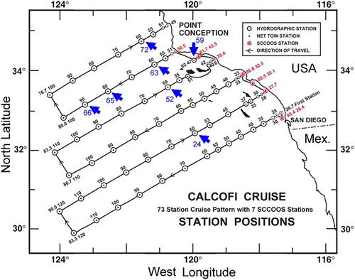
Table 1. CalCOFI stations discussed in this paper. Cross-slope (59, 63, 65, and 66) and along-slope (24, 52, 63, and 72) station locations are identified in Fig. 4.

Station Consec. no.	Line no. Along-Shelf	Line no. Cross-Shelf	Latitude (°N)	Latitude Range of Data (°N)	Longitude (°W)	Longitude Range of Data (°W)	Bottom Depth (m)
59	81.8	46.9	34.27	34.13–34.30	120.03	119.92–120.15	578
63	80	60	34.15	34.05–34.25	121.15	121.05–121.27	2204
65	80	80	33.48	33.40–33.55	122.53	122.43–122.60	4007
66	80	90	33.15	33.06–33.25	123.22	123.12–123.29	4229
24	90	60	32.42	32.36–32.48	120.00	119.90–120.10	880
52	83.3	60	33.58	33.40–33.69	120.75	120.60–120.90	1397
72	76.7	60	34.72	34.60–34.80	121.55	121.40–121.67	930

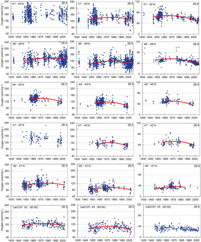
Scatterplots of all O₂ observations and their significant quadratic polynomials (red trend lines) at the four cross-slope locations are presented in Fig. 5. Despite the variability in the data, decadal trends of O₂ shown by these polynomials follow a similar doming pattern at all stations, with maximum O₂ in the middle decades and minimum O₂ at the beginning and end of the time periods. The maxima in O₂ are 13 to 16 μmol kg⁻¹ greater than the minima. Even in the Southern California Bight (station 59) where O₂ is significantly lower, the same pattern of increasing O₂ is seen from the 1950s to about 1980 and decreasing O₂ afterwards to the end of the data series. The temporal pattern is similar to that found by McClatchie et al. (2010) on the 26.6 σ _θ surface for a region to the south and inshore of most of our stations and by Koslow et al. (2011) over most of the CalCOFI stations but over the depth range of 200 to 400 m rather than on constant σ _θ surfaces.

Fig. 5 Scatterplots of observations of O₂ (left, μmol kg⁻¹) and Θ (middle, °C) interpolated onto the 26.7 σ_θ surface at four CalCOFI stations. Depth of the 26.7 σ_θ surface is plotted in the right column. Blue symbols represent individual observations. Red lines are significant quadratic polynomials of annual averages of O₂. Black lines are best-fit quadratic polynomials to all observations of Θ and depth of the 26.7 σ_θ surface. Horizontal axes show the year of observation.

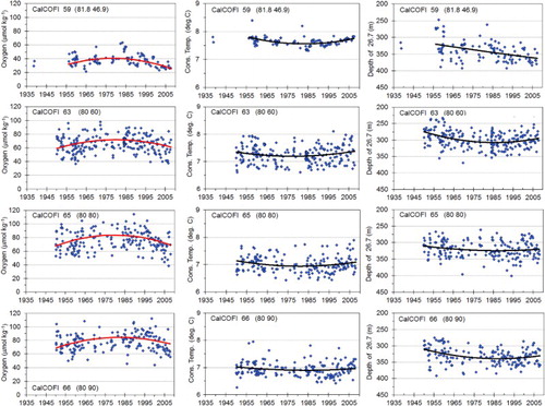
Crossing the continental slope, typical trend lines of O₂ range from 28 to 41 μmol kg⁻¹ closest to shore in the Southern California Bight at station 59, increasing to a range of 59 to 72 μmol kg⁻¹ at station 63; 68 to 84 μmol kg⁻¹ at station 65; and 69 to 85 μmol kg⁻¹ at station 66 (Fig. 5). Accompanying this spatial change in O₂ is a decrease in Θ with increasing distance offshore. (Changes in S_A correlate almost perfectly with Θ on constant density surfaces and are not presented or discussed for this reason.) The shallowest depth of the 26.7 σ _θ surface is at station 63, one of the locations identified by Gay and Chereskin (2009) to lie in the core of the CUC.

The depth of the 26.7 σ_θ surface and Θ follow the inverse temporal trend of O₂, except in the Southern California Bight (station 59) where a linear increase in depth of the 26.7 σ _θ surface is present. The correlation coefficient between annual averages of Θ and O₂ is −0.4 at station 59, and −0.8 at the three stations farther offshore. The negative correlation of temperature and O₂ is of the same sign as noted by Deutsch et al. (2011) in waters to the south of the CalCOFI region. Meinvielle and Johnson (2013) also note that decreasing O₂ after 1980 was accompanied by higher salinity and temperature (spicier) in this region on the shallower 26.5 σ _θ surface. Their study did not evaluate details of O₂ changes prior to 1980. Meinvielle and Johnson (2013) observed increasing spiciness after 1980 all through their domain but note that results north of 40°N should be treated with caution. Nonetheless, when analyzing percentage O₂ saturation instead of O₂ concentration, decadal trends in O₂ similar to those presented in Fig. 5 were obtained, indicating that temperature-related solubility of O₂ is not the primary cause of its decadal variability.

Observations of O₂ at the three additional stations along the continental slope (72, 52, and 24) have similar decadal variability in O₂ as observed at the across-slope stations (data not shown), with the exception of station 24 where doming was weaker than noted elsewhere. The concentration of O₂ co-varied inversely with Θ and the depth of the 26.7 σ _θ surface at these three additional stations, just as found at the four cross-slope stations.

2 Continental slope from California to Vancouver Island

The four 1-degree-latitude bands selected for analysis are 36°–37°N, 41°–42°N, 44°–45°N, and 48°–49°N. Sampling has been less regular in these regions than in the CalCOFI region, especially along the three southern lines. At each of the four latitude bands, decadal trends in O₂ shown by the significant quadratic polynomial curves in Fig. 6 follow a doming pattern similar to that of the CalCOFI region, with maximum O₂ in 1975 to 1982. Oxygen generally increases towards the north, with the peak concentration increasing by 40 µmol kg⁻¹ from 36°–37°N to 48°–49°N. There appears to be some change in the magnitude of temporal doming with latitude, which is discussed later.

Fig. 6 Scatterplots of observations of O₂ (left, μmol kg⁻¹) and Θ (middle, °C) interpolated onto the 26.7 σ_θ surface, for locations on the continental slope between 36°N (bottom panels) and 49°N (top panels) where the bottom depth is between 210 and 1500 m. Depth of the 26.7 σ_θ surface is plotted in the right column. Blue symbols represent individual observations. Red lines are significant quadratic polynomials of annual averages of O₂. Black lines are best-fit quadratic polynomials to all observations of Θ and depth of the 26.7 σ_θ surface. Horizontal axes show the year of observation.

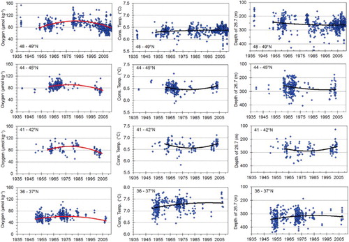
There is no consistent relationship between Θ and O₂ or between the depth of the 26.7 σ _θ surface and O₂ among these four latitude bands (Fig. 6). Whereas in the CalCOFI region both Θ and the depth of the 26.7 σ _θ surface vary inversely with O₂ in the pairs of time series across the continental shelf, in these four northern latitude bands negative co-variation is found only at 41°–42°N and 44°–45°N. The depth of the 26.7 σ _θ surface decreases to the north, from an average of 300 to 350 m in the CalCOFI area, to about 250 m at 48°–49°N.

3 Northern British Columbia

Sampling in regions to the north of Vancouver Island has been irregular since the earliest measurements in the 1930s, with relatively few observations on the continental slope. Therefore, observations across a wide range of latitude and longitude were considered, from 51°–55°N and 131°–137°W, as plotted in Fig. 7. Two different sub-regions were investigated to determine any impact of different trends in deep-sea and shelf waters. One sub-region covered the area 51°–54°N, 128.7°–135.8°W and the other 5°–55°N, 133.6°–135.0°W. Although there were fewer samples, and the magnitude of doming of O₂ varied somewhat from the larger region, the general features were similar, and results are presented only for the range 51°–55°N and 131°–137°W.

Fig. 7 Locations of O₂ observations on the 26.3 σ_θ surface for the Gulf of Alaska north and west of Haida Gwaii (formerly the Queen Charlotte Islands) of the northwest coast of Canada. Symbol colours denote the decade of sampling. Grey and black lines are the 200 and 1500 m isobaths, respectively.

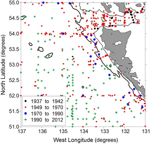
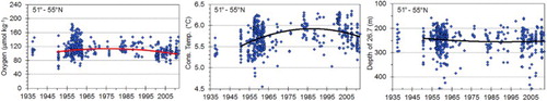
There were relatively few samples taken prior to 1949 or from 1970 to 1990. Although in Fig. 7 there appear to be few samples shoreward of the 1500 m isobath after 1990, this is not the case because many of these locations were sampled several times during repeat surveys, resulting in only one plotted symbol. The trend line for O₂ (Fig. 8) ranges from 97 to 113 μmol kg⁻¹ compared with the trend line range of 78 to 102 μmol kg⁻¹ at 48°–49°N. On average, Θ increased by almost half a degree until about 1990 then it declined slightly, whereas the depth of the 26.7 σ _θ surface experienced minor changes. The 26.7 σ_θ surface has an average depth of about 250 m, comparable with that at 48°–49°N.

Fig. 8 Scatterplots of observations of O₂ (left panel, μmol kg⁻¹) and Θ (middle panel, °C) interpolated onto the 26.7 σ_θ surface, for the region to the north and west of Haida Gwaii (formerly the Queen Charlotte Islands) (51°–55°N, 131°–137°W). Depth of the 26.7 σ_θ surface is plotted in the right panel (m). Blue symbols represent individual observations. Red lines are significant quadratic polynomials of annual averages of O₂. Black lines are best-fit quadratic polynomials to all observations of Θ and depth of the 26.7 σ_θ surface. Horizontal axes show the year of observation.

4 Other σ _θ surfaces along the continental slope

To this point we have presented results only for the 26.7 σ _θ surface to allow visual comparison among the many regions considered. However, this approach limits our understanding of impacts, especially on the continental shelf where the 26.7 σ _θ surface may not penetrate onto the shelf in some locations or may only penetrate during summer months. Therefore, additional results are examined here for the 26.3, 26.5, and 26.9 σ _θ surfaces. Figure 9 presents scatterplots of O₂ versus year of observation and their significant quadratic polynomials on these three σ _θ surfaces along the continental margin, from CalCOFI station 63 at 34°N to the northern British Columbia region at 51°–55°N.

Fig. 9 Scatterplots of observations of O₂ (μmol kg⁻¹) versus year for three σ_θ surfaces: 26.3 (left), 26.5 (middle), and 26.9 (right), at locations along the continental slope from southern California to southern British Columbia and on the continental margin for the most northern region at 51°–55°N. Blue symbols represent individual observations. Red lines are significant quadratic polynomials of annual averages of these observations. Stations where no significant quadratic polynomials were found do not have red lines. Horizontal axes show the year of observation. Note the change in scale for O₂ on the 26.9 σ_θ surface.

As observed for the 26.7 σ _θ surface, O₂ generally increases northward of 36°–37°N on each σ _θ surface. The scatter in observations decreases with depth, with much less scatter on the deeper 26.9 σ _θ surface than on the 26.3 and 26.5 surfaces. Significant doming is observed in all but three locations and density ranges. A feature of these significant quadratic polynomials, shared with those on the 26.7 σ _θ surface, is that that the maximum O₂ concentration along the continental slope occurred around 1980.

5 o₂ Trends along the continental slope

We next present the combined results of the statistical analyses of the annual-average O₂ observations and correlations among time series of annual-average O₂ and Θ at all twelve locations examined: seven locations in the CalCOFI region and five latitude bands along the continental slope at more northern latitudes.

The time series of significant quadratic polynomials of O₂ are presented in Fig. 10 for all four σ _θ surfaces. Each graph begins in 1950, a common start year of many series. Each series in Fig. 10 spans only the years for which annual averages are available, defined as three or more observations in a year. At northern locations over the range of σ _θ surfaces from 26.3 to 26.9, statistically significant doming is found at 3, 5, 5, and 5 locations, respectively. This differs from the CalCOFI stations, where doming is found at 6, 7, 4, and 2 σ _θ surfaces from 26.3 to 26.9, respectively. Therefore, the doming appears to be most robust for the CalCOFI stations at σ _θ of 26.5 and 26.3, but at σ _θ of 26.5 to 26.9 at northern stations. For all twelve locations, O₂ peaks between the years 1976 and 1982 with a few exceptions.

Fig. 10 Significant quadratic polynomials of annual averages at each station and region. Panels are for the following σ_θ surfaces: (a) 26.3, (b) 26.5; (c) 26.7; and (d) 26.9. (left panel) Northern stations from 36°N to 55°N and (right panel) CalCOFI stations.

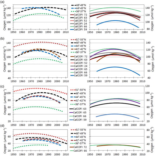
The range of doming varies among these σ _θ surfaces. To compare among series with different start and end years, we selected a common range of years from 1960 to 2005. The largest doming among all twelve series is found at the three northern latitude ranges from 41°–49°N, averaging 18 μmol kg⁻¹ on each of the 26.5 and 26.7 σ _θ surfaces, and 12 and 11 μmol kg⁻¹ on the 26.3 and 26.9 σ _θ surfaces, respectively. In comparison, doming averages between 9 and 11 μmol kg⁻¹ at 36°–37°N, and only 8 μmol kg⁻¹ at 51°–55°N. At the CalCOFI stations, at nominal distances of 60 km from the coast, average doming magnitude is 11, 14, 8, and 5 μmol kg⁻¹ on the 26.3 to 26.9 σ _θ surfaces.

At the CalCOFI stations the increase in average O₂ with distance from shore can be easily seen, with the lowest O₂ at station 59 in the Southern California Bight and highest O₂ at stations 65 and 66 farthest offshore. Three CalCOFI stations along the CUC, numbered 63, 52, and 24, generally exhibit similar magnitudes and O₂ variability on each of the four σ _θ surfaces. Our results are similar to those of McClatchie et al. (2010), with temporal domes of about 13 μmol kg⁻¹ on the 26.7 σ _θ surface in our CalCOFI region compared with about 10 μmol kg⁻¹ for McClatchie et al. (2010) on the 26.6 σ _θ surface at stations that are mostly closer to shore. Koslow et al. (2011) examine O₂ at constant depth rather than on constant σ _θ surfaces, so their results do not correspond to ours. Bograd et al. (2015) examine changes in spiciness, nutrients, and O₂ on the 26.5 σ _θ surface at CalCOFI stations for the years 1984 to 2012, finding that decreases in O₂ and increases in nitrate (NO₃) are generally greater at offshore CalCOFI stations than inshore stations. Offshore changes seem to be associated with advection in the North Pacific Subarctic Gyre.

Although O₂ generally increases on constant density surfaces in the CUC from south to north, the trend is not uniform along the coast. If the northern stations are compared with the four CalCOFI stations, 72, 63, 52, and 24, that lie generally along the CUC, the lowest O₂ is found in the 36°–37°N latitude band on the 26.5 and 26.7 σ _θ surfaces. For example, on the 26.7 σ _θ surface, maximum O₂ is 61 μmol kg⁻¹ at 36°–37°N and 71 μmol kg⁻¹ at CalCOFI station 63. By comparison, on the same σ _θ surface, the temporal domes in O₂ at the four latitude bands to the north of 36°–37°N range from 90 to 114 μmol kg⁻¹. However, on the 26.9 σ _θ surface, O₂ is similar at CalCOFI stations in the CUC and at 36°–37°N, reaching a peak concentration of 36 μmol kg⁻¹. At northern locations, the increase in O₂ on the 26.9 σ _θ surface at latitudes to the north of 36°–37°N is still present, with temporal O₂ peaks ranging from 52 to 69 μmol kg⁻¹.

Correlations between changes in time of annual averages of observed O₂ and Θ were computed to provide insight into other aspects of seawater changes in time. These correlations were high in magnitude at CalCOFI stations, averaging −0.8 on the 26.5 and 26.7 σ _θ surfaces, −0.7 on the 26.3 σ _θ surface, and −0.4 on the 26.9 σ _θ surface. Correlations averaged about −0.2 on each density surface at the five northern locations, with the smallest absolute magnitudes occurring at 48°–49°N and 51°–55°N. This drop in correlation at northern locations is important because it suggests that different processes likely account for decadal change in O₂ north of the CalCOFI region.

We examined the slope of the relationship between annual averages of O₂ and Θ along the continental margin to investigate the possible impact of the temperature-dependent O₂ solubility on this O₂ doming in time, focusing on locations where the square of the correlation coefficient (R²) between O₂ and Θ exceeded 0.5. At all seven stations in the CalCOFI region on the 26.5 and 26.7 σ _θ surfaces, changes in O₂ are correlated (R² > 0.5) with changes in Θ, and the slope of the relationship exceeded the slope of the temperature-dependent O₂ solubility by factors ranging from 6 to 13. Only three stations met the R² > 0.5 test on the 26.3 σ _θ surface, with slopes exceeding the temperature-dependent O₂ solubility slope by factors of 7 to 11. Only one station on the 26.9 σ _θ surface qualified, and the factor there is 5. Therefore, the impact of temperature-dependent O₂ solubility on temporal doming is present but is a minor cause of the temporal doming of O₂ and of correlations between O₂ and Θ.

A final comment relevant to the next section is that there is little evidence along the continental slope of cyclical variability in O₂ at the period of the 18.61-year LNC. Only the O₂ observations at 48°–49°N on the 26.9 σ _θ surface were found to fit the LNC with 95% confidence. Such variability was noted in previous studies of O₂ at OSP in deep-sea waters of the Gulf of Alaska and is presented in the next section. The variability of LNC at 48°–49°N has a much smaller amplitude and larger phase shift compared with the signal 1000 km offshore. Therefore, we suspect that this LNC signal on the slope is locally generated.

b Deep-Sea

Observations of O₂ are presented along several sections of the Northeast Pacific Ocean where repeat measurements were made in several decades, as well as at OSP where nearly continuous measurements are available from 1956, and at other main stations along Line P.

1 East–west section along line P

In deep-sea waters the time series most suitable for statistical evaluation are from the five main stations that lie along Line P (Fig. 3e). The station farthest offshore is OSP where regular sampling began in 1956. Oxygen at four other deep-sea stations to the east has been regularly sampled since 1981 by Canadian research surveys heading to and from OSP: P20 (49.57°N, 138.67°W), P16 (49.28°N, 134.67°W), P12 (48.97°N, 130.67°W), and P8 (48.82°N, 128.67°W). Bottom depth at P8 is 2440 m; depths at the other stations are more than 3000 m. Station P4 lies on the continental slope and its observations are included in the region at 48°–49°N presented previously.

We added nearby observations to the time series at P8, P12, P16, P20, and OSP. The search for observations at each station extended east and west approximately halfway to its neighbouring Line P station and north and south from 48.5°N to 51.0°N. These additional observations extended the time series back in time to 1950, except at OSP where no useful observations prior to 1956 were found. Scatterplots of O₂ observations at four of these Line P stations are shown in Fig. 11 for the σ _θ surfaces 26.5, 26.7, and 26.9. Station P12 is not presented in Fig. 11 because it is similar to the O₂ scatterplot at P8.

Fig. 11 Oxygen concentration interpolated onto three σ_θ surfaces at four stations along Line P: (a) OSP at 50.00°N, 145.00°W; (b) P20 at 49.57°N, 138.67°W; (c) P16 at 49.28°N, 134.67°W; and (d) P8 at 48.82°N, 128.67°W.

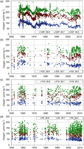
The graph for OSP, Fig. 11a, closely matches the time series on these density surfaces presented by Whitney et al. (2007), with additional observations included because of sampling at neighbouring stations and after 2006. The time series for P20, P16, and P8 have not been previously published. Several features of these observations can be readily noted. The scatter of individual observations decreases with increasing density, as well as with distance offshore. A linear trend appears to dominate on the two densest surfaces at OSP, whereas a doming trend in time seems to dominate at P8. Statistical analyses of these trends are presented later.

In addition, all of these time series show considerable decadal variability. Andreev and Baturina (2006), Whitney et al. (2007), and Falkowski et al. (2011) note that a lunar-origin signal of period 18.61 years appears to fit the time series of O₂ on the 26.9 σ _θ surface at OSP. Similar variability is noted in the western North Pacific where it is attributed to the LNC that modulates tidal mixing in the formation region of North Pacific Intermediate Water (Yasuda et al., 2006). Osafune and Yasuda (2013) successfully simulate this 18.6-year cycle in a numerical model of the North Pacific Ocean. Although the LNC appears in atmospheric data for western North America, its source is believed to be the northwest Pacific Ocean (McKinnell & Crawford, 2007). Statistical analysis of LNC variability is presented later.

Some observations of unusually low O₂ in Fig. 11 are attributed to Haida or Sitka eddies, such as those at P16 in 1992, 1995, and 1998. Mesoscale eddies can be found in images of sea surface height anomaly based on satellite altimetry after 1992, which reveal that these eddies were most frequent near P16 and less common at other Line P stations (Ladd, 2007). The two anomalies at OSP in 1960 and 1974 are likely due to Haida or Sitka eddies as well (Whitney et al., 2007), but because they predate the era of satellite altimetry we cannot offer independent confirmation. No large mesoscale eddies have been identified in satellite altimetry at OSP since regular observations began in 1992 with the launch of the TOPEX/Poseidon satellite although several weak eddies were sampled at sea near OSP in July 2002.

Oxygen experiences larger scatter at P8 (Fig. 11d) and also at P12 (not shown), perhaps because of the stirring of coastal and deep-sea waters. California Undercurrent Eddies (Cuddies) transit past these two stations. Cuddies are almost entirely subsurface, generally centred between the 26.0 and 26.8 σ _θ surfaces, carrying CUC water westward from the continental slope (Pelland et al., 2013). Like other subsurface eddies, they cannot be detected using satellite altimetry. Their effect emerges in calculations of co-variability of O₂ and Θ, presented next.

Temperature changes along the constant density surfaces show different patterns along Line P. A measure of this co-variability is the correlation coefficient between O₂ and Θ. All observations were input to this calculation of co-variability, rather than annual averages as input for calculations along the continental margin because the transit time of eddies past any single Line P station is less than a year. Although correlations are negative at all stations and densities, their magnitudes increase toward shore. The correlation coefficients on the 26.7 and 26.9 σ _θ surfaces at OSP are only −0.2 and are somewhat larger in magnitude on the 26.5 σ _θ surface. In the sequence of stations P20, P16, P12, and P8 the average correlations on the three σ _θ surfaces are −0.3, −0.5, −0.6, and −0.8, respectively. This pattern reveals the increasing influence of transient eddies on the temperature and O₂ concentrations as stations approach the continental slope. Haida Eddies dominate at P16 and Cuddies at P12 and P8. The large magnitude of the correlation coefficient at P8 reveals that the very large scatter among individual observations of O₂ at P8 (Fig. 11d) is not random but instead could be a result of the presence or absence of Cuddies. The dominance of eddies is missing on the continental slope itself, where the correlation of O₂ and Θ over individual observations decreases in magnitude to an average of −0.2 for the 48°–49°N range of latitudes.

We next present results from temporal trend analyses, including best fit and confidence limits for quadratic and linear trends as well as the 18.61-year oscillation at all five deep-sea Line P stations.

i Temporal doming

A quadratic trend was found to be significant at the 95% confidence level on the 26.7 and 26.9 σ _θ surfaces at P8 and on the 26.7 σ _θ surface at P12 but not in any other time series. The peaks in O₂ occurred between 1975 and 1981, with doming of about 20 μmol kg⁻¹ on the 26.7 σ _θ surface and 10 μmol kg⁻¹ on the 26.9. Timing of the peak and the magnitude of the temporal doming are close to those of stations on the continental slope. Distance to the 200 m isobath of the continental slope is 150 km at P8, 250 km at P12, and 430 km at P16, so the region along the continental slope where O₂ increases from the 1950s to about 1980 extends to somewhere between 250 and 430 km offshore at the latitude of Line P.

ii Linear trend

The slope of the linear trend at Line P stations and at 48°–49°N is presented in Table 2a. The time series at 48°–49°N is included to compare results from deep-sea Line P stations with observations on the nearby continental slope. All three σ _θ surfaces at OSP show significant linear decreases of O₂ in time, with values of −0.39 to −0.50, somewhat smaller than determined by Whitney et al. (2007) for the same density surfaces. Some of the difference can be explained by the years of observations examined; Whitney et al. (2007) included observations up to mid-2006 at OSP, whereas our time series extend to 2011 during a time of increasing O₂ on these σ _θ surfaces. Our use of annual averages redistributes the weighting somewhat. In general, linear slopes are smaller and less robust at other Line P stations. A slope of −0.52 μmol kg⁻¹y⁻¹ is present at P20 on the 26.5 σ _θ surface, but elsewhere the slopes are smaller in magnitude, at rates ranging from −0.14 to −0.24 μmol kg⁻¹y⁻¹, and confined to the 26.9 σ _θ surface at stations between P16 and 48°–49°N. The decrease on the 26.9 σ _θ surface at 48°–49°N is visually comparable to the decrease at 41°–42°N, 44°–45°N, and 51°–55°N, as can be seen in Fig. 10d.

Table 2. Properties of the annual-average Line P time series of O₂ on σ_θ surfaces. The 95% confidence limits are in parentheses. Table 2a lists the slope of the linear trend. Trends are not listed if the confidence limit exceeds the magnitude of the slope. Table 2b lists the amplitude and phase of the best-fit 18.61-year LNC to each time series for the 26.9 surface.

(a)	Linear Trend (μmol kg^−1 y^−1)
σθ	48°–49°N	P8	P12	P16	P20	OSP
26.9	−0.24 (±0.11)	−0.18 (±0.12)	−0.15 (±0.07)	−0.14 (±0.10)	–	−0.39 (±0.15)
26.7	–	–	–	–	–	−0.50 (±0.26)
26.5	–	–	–	–	−0.52 (±0.37)	−0.41 (±0.28)
(b)	Lunar Nodal Cycle (LNC) Amplitude (μmol kg^−1) and Phase (years)
σθ	48°–49°N	P8	P12	P16	P20	OSP
26.9 Ampl	4 (±2)	4 (±2)	3 (±2)	18 (±2)	18 (±1)	18 (±1)
26.9 Phase	3.8 (±2.5)	4.0 (±3.5)	2.4 (±1.7)	3.8 (±2.6)	11.8 (±4.6)	11.9 (±3.5)

At OSP the decline in O₂ on the three σ _θ surfaces was rapid from 1995 to about 2003 with a magnitude of approximately 50 μmol kg⁻¹. Similar declines were found at P20 and P16 on the 26.7 and 26.9 σ _θ surfaces, although the decline started and ended sooner. The timing and magnitude of this decrease coincide with a rapid drop in O₂ found elsewhere in deep-sea waters of the Gulf of Alaska and are discussed in later sections that examine changes in O₂ away from Line P.

iii LNC variability

The amplitude and phase of the LNC cycle are shown in Table 2b. The most significant LNC variability is found on the 26.9 σ _θ surface. Variability at OSP and P20 share the same phases and amplitudes, but the phase shifts by 8 to 10 years at the more eastern stations, which is about a half cycle of the 18.61-year LNC. In addition, the amplitude decreases from 18 μmol kg⁻¹ at OSP and P20 to only 3 to 4 μmol kg⁻¹ at stations from P12 to the continental slope. Clearly, deep-sea processes driving the LNC-period variability are not penetrating eastward of station P20, and station P16 displays a curious mix of amplitudes and phases of neighbouring stations. Haida Eddies transit through P16 frequently and seldom arrive at neighbouring stations (Ladd, 2007), so it is not surprising that the deep-sea LNC phase at OSP and P20 is different at P16. More easterly Line P stations are in the realm of the continental shelf and slope domain. This boundary is defined by Klymak, Crawford, Alford, MacKinnon, and Pinkel (2015), who examined variability of potential temperature and spice (a measure of co-variability of temperature and salinity on constant density surfaces) along Line P based on closely spaced sampling in August 2008 by a continuously measuring towed profiler. They established that the boundary between coastal and deep-sea waters is between stations P12 and P16.

2 East–west section along 47°N

Sampling took place along 47°N in the 1980s, 1990s, and 2000s, along with irregular sampling in previous decades (Fig. 3d). This is identified as World Ocean Circulation Experiment (WOCE) Line P1, which extends westward across the entire North Pacific Ocean. Our sampling extended north and south of 47°N by 0.5° of latitude and from the 210 m isobath in the east to 170°W. Along this transect, O₂ and Θ observations are clustered into three periods in Fig. 12: 1955 to 1985, 1999, and 2005 to 2007. Because changes in O₂ during the three decades of 1955 to 1985 did not show a general trend, all observations from these years are combined.

Fig. 12 (a) O₂ and (b) Θ measured on WOCE line P1 along 47°N on the 26.7 σ_θ surface for each of three periods. Green lines in (a) indicate stations most likely to have been affected by a Haida Eddy.

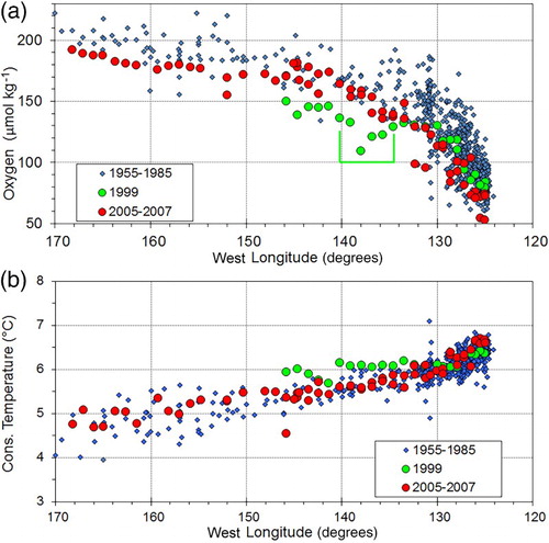
Along 47°N, a major drop in O₂ is found between 136°W and 146°W in 1999, with lower O₂ than in all previous years (Fig. 12a). These low O₂ values are accompanied by higher Θ, as shown in Fig. 12b. A previous examination of these measurements (Crawford, 2005) determined that in June 1999 a massive Haida Eddy named Haida 1998 was located just to the north, centred at 47.53°N, 137.46°W. This eddy was detected in anomalies of temperature for six stations along the transect and also in images of sea surface height anomaly based on satellite measurements. These six stations are bracketed by the green line in Fig. 12a.

Haida Eddies form on the continental slope along the west coast of Haida Gwaii in northern British Columbia and propagate mainly westward although their motion varies from northwest to due south. Haida 1998 is the largest Haida eddy observed to date (Crawford, 2002) and the only one to be tracked as far south as 47°N. A general feature of these eddies is that their core waters below 100 m are warmer, saltier, and lower in O₂ than background seawater of the same density (Crawford, 2002; Ladd, Stabeno, & Cokelet, 2005). We believe the extreme anomalies in O₂ and Θ along these six stations in June 1999 can be attributed to Haida 1998. Five stations to the west of Haida 1998 are also relatively lower in O₂ and higher in Θ than almost every previous observation. A few stations to the east of Haida 1998 are generally low in O₂ (but not the lowest on record) and high in Θ. We cannot assess the extent to which Haida 1998 might have influenced O₂ and Θ at these neighbouring locations. The coincidence of both O₂ and Θ anomalies suggests the eddy may have affected these outer stations, but the weather systems shifted significantly between spring 1998 and summer 1999 and also changed subsurface currents and water properties (Donohue & Stacey, 2013), which could have changed O₂ and Θ along WOCE line P1.

The most recent period presented in Fig. 12, from 2005 to 2007, shows a decrease in O₂ at all longitudes compared with the period 1955 to 1985, with decreases ranging from 10 to 30 μmol kg⁻¹. Although not shown in Fig. 12, O₂ on the 26.9 σ _θ surface also decreased in 2005 to 2007, but changes on the 26.5 σ _θ surface were minor. Observations west of 145°W in 2005 to 2007 are from 2007 only, whereas both 2005 and 2007 contribute to observations to the east of 145°W. Sampling in 2006 was from about 128°W to 130°W, with two additional stations at 152°W.

Some of the decrease in O₂ observed between the two periods of 1955 to 1985 and 2005 to 2007 could be a result of irregular sampling in the 18.61-year LNC. This variability is most evident at OSP and P20, as discussed earlier, which are only three degrees of latitude to the north of 47°N. If LNC variability along Line P is also present along 47°N, then the timing of the sampling along 47°N may have caused some of the decrease in O₂ noted above. Along 47°N and west of 130°W on the 26.7 and 26.9 σ _θ surfaces, less than 2% of the samples taken between 1955 and 1985 were collected during the period of very low O₂ at OSP from 1967 to 1971, which coincided with a negative phase of the LNC; therefore, these observations may be biased to high O₂. In contrast, the years 2005 to 2007, with very low O₂, coincide with a negative phase of the LNC and may be biased to low O₂. The range of the LNC in O₂ on the 26.7 σ _θ surface at P20 and OSP is comparable to the decrease along 47°N between the two ranges of years 1955–1985 and 2005–2007. Therefore, the decrease in O₂ along WOCE line P1 east of 170°W may be linked to the LNC as well as a general decrease in O₂.

3 North-south section between 149.5°W and 161.2°W

Stations within the longitude range of 149.5°W to 161.2°W (Fig. 3c) include repeat tracks considered by Mecking et al. (2008), a north–south section along 155°W in 1985, and irregular sampling throughout the record, especially from 1949 to 1980. Depths of the 26.7 σ _θ surface are used to determine the location of measurements relative to the North Pacific Current, Alaskan Gyre, and Alaskan Stream. These depths range from an average of 500 to 600 m in the North Pacific Current at 30°N to a minimum of about 150 m in the middle of the Alaskan Gyre at 53°N, and 200 to 300 m in the Alaskan Stream, which lies north of about 55°N. All observations where bottom depth was shallower than 210 m were excluded to eliminate samples from the Alaskan continental shelf at the north end of this section. Oxygen and Θ on the 26.7 σ _θ surface along this section are plotted in Figs 13a and 13b, respectively, for several time periods. The latitude of minimum Θ is close to 53°N at mid-gyre.

Fig. 13 Observations of (a) O₂ and (b) Θ along a north–south section in the Northeast Pacific Ocean from 149.5°W to 161.2°W, excluding samples where bottom depth is less than 210 m. All values have been interpolated onto the 26.7 σ_θ surface. Colours denote time intervals as shown in the legends.

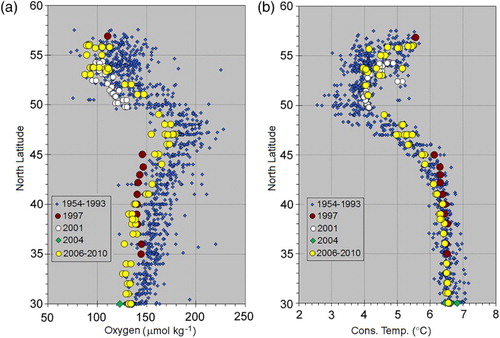
We first grouped the early observations into several periods based on years of relatively high and low O₂ at OSP to search for evidence of the LNC (Fig. 11a): 1954 to 1966, 1967 to 1971, and 1972 to 1993. Very similar O₂ was observed at all latitudes in the first and third periods. The middle period of 1967–1971 is an era of low O₂ at OSP. Unfortunately, although O₂ is somewhat lower, there are too few observations in these five years between 149.5°W and 161.2°W to determine whether a significant minimum exists. Therefore, all observations from 1954 to 1993 are grouped together in Fig. 13. After 1993 almost all the observations fall into four time spans: 1997, 2001, 2004, and 2006 to 2010, and their values are plotted in Fig. 13 with distinct symbols. Samples in 1997 were from 35°N to 45°N and at 57°N; those in 2001 were collected between 50°N and 55°N; those in 2004 were all at or near 30°N; observations in 2006 to 2010 were from the entire latitude range of 30°N to 57°N. Oxygen in each of these four recent periods was lower than in the period from 1954 to 1993 (Fig. 13a).

Observations from 2006 to 2010 span the full latitude range and are clearly lower in O₂ (Fig. 13a). To investigate the statistical significance of this difference in O₂ between the two periods 1954 to 1993 and 2006 to 2010, we computed means and twice the standard errors of each time series in five different latitude bands, each extending over 5°. The range of ±2 standard errors approximately encloses the 95% confidence limits of the mean. No differences were computed in the latitude range 50° to 53°N where the change in O₂ with latitude is rapid. Results are listed in Table 3. In every latitude band the ranges of ±2 standard errors about the sample means of the two periods do not overlap, indicating very significant differences in O₂ between the two periods. The decrease in mean O₂ in the 5° latitude bands varies from a low of 11 μmol kg⁻¹ at 45° to 50°N to a high of 23 μmol kg⁻¹ at 53° to 58°N. Similar calculations for the more spatially limited observations in 1997, 2001, and 2004 also reveal decreases in O₂ from the 1954 to 1993 averages.

Table 3. Statistically significant differences in O₂ (μmol kg⁻¹⁾ between the two periods 1954–1993 and 2006–2010 in the longitude range 149.5°–161.2°W. Columns for each period list the mean, the mean plus two standard errors, and the mean minus two standard errors. Numbers in bold indicate the lower limit for 1954–1993 and the upper limit for 2006–2010. The right column lists differences in the means.

	1954 to 1993			2006 to 2010
Latitude Band	Mean Plus 2 Standard Errors	Mean	Mean Minus 2 Standard Errors	Mean Plus 2 Standard Errors	Mean	Mean Minus 2 Standard Errors	1954 to 1993 Minus 2006 to 2010
30°–35°N	149	147	146	132	131	130	16
35°–40°N	160	158	156	138	137	136	21
40°–45°N	172	170	167	160	157	155	13
45°–50°N	186	183	180	174	172	170	11
53°–58°N	125	123	122	103	100	96	23

Mecking et al. (2008) examined measurements along 152°W in great detail for the repeat sections of 1980, 1984, 1991, 1997, and 2006. Emerson, Mecking, and Abell (2001) and Emerson et al. (2004) examined changes along north–south lines at 152°W and 158°W in the 1980s and 1990s. These studies provide extensive insight into factors related to O₂ changes since 1980. Our comparison reveals that the magnitude of the decrease in O₂ after 1993 exceeds the magnitude of any change in O₂ in previous decades back to 1954.

Observations of Θ are presented in Fig. 13b for the same periods as O₂ in Fig. 13a. In general, Θ shows a much less organized decadal variability than does O₂. Compared with Θ of 1954 to 1993, Θ was somewhat higher in 2001 and in 2006–2010 from 50° to 57°N, suggesting a negative correlation with O₂ over the full time series in this latitude range. Elsewhere, changes in Θ are relatively small. Therefore, a consistent relationship between O₂ and Θ at all latitudes is not present. Declines in O₂ on the 26.9 and 26.5 σ _θ surfaces are generally similar to those on the 26.7 σ _θ surface; however, north of 45°N there is some evidence of local mixing on the 26.5 σ _θ surface with O₂-enriched surface waters.

4 WOCE line P17

A section of north–south stations was sampled between 1991 and 2001 along WOCE Line P17 (Fig. 3f), with results presented in Fig. 14. Along this section, O₂ on the 26.7 σ_θ surface dropped by about 20 to 60 μmol kg⁻¹ from 1993 to 2001 at latitudes between 40°N and 52°N and by about 20 µmol kg⁻¹ from 52°N to 55°N. From 30°N to 32°N the drop was of order 10 µmol kg⁻¹ from 1991 to 2001. At 50°N the decrease was 55 μmol kg⁻¹, similar to the decrease of about 50 μmol kg⁻¹ at OSP from 1995 to 2003 noted previously. The decline from 1995 to 2003 is in phase with the decrease in O₂ observed at OSP, where it is in phase with the LNC decrease. North of 50°N WOCE Line P17 lies within the region presented in Section 4.b.3 at 149.2°W to 162.5°W, and the decline in O₂ is similar for these two sections where sampling overlaps in space.

Fig. 14 Observations of (a) O₂ and (b) Θ on WOCE line P17 between 1991 and 2001 on the 26.7 σ_θ surface. The section extends northward along 135°W to 41°N, then heads towards 55°N, 159°W, as shown in Fig. 3f.

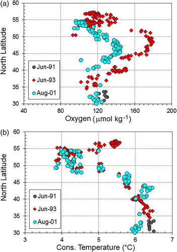
There is no consistent relation between O₂ and Θ changes (Fig. 14b), and at latitudes where O₂ decreased most, Θ changes were minor. Declines in O₂ on the 26.9 and 26.5 σ _θ surfaces are generally similar to those on the 26.7 σ _θ surface, with a similar lack of consistency to changes in Θ.

4 Summary and conclusions

We examined observations of O₂ concentration and Θ in regions of the Northeast Pacific Ocean and along the continental margin, focusing on specific stations and regions where observations have been made in most decades since the late 1940s and are included in NODC and Canadian archives. Stations and regions on the continental slope were seaward of the 210 m isobath, generally coinciding with the location of the CUC. We selected seven stations sampled by CalCOFI in southern California, four regions along the continental slope between 36° and 49°N, and a final region on the continental margin from 51° to 55°N. In deep-sea regions we selected OSP, as well as other offshore stations along Line P. In addition, we included observations along WOCE lines P1 and P17 and along a north–south line of stations between 149.5° and 161.2°W. Archived values were interpolated onto several σ _θ anomaly surfaces, with most effort focused on the 26.7 σ _θ surface. Our main findings follow.

A decrease in O₂ was observed at all locations from about 1980 to the 2000s. On the continental margin this decline was preceded by an increase in O₂ from the 1950s to about 1980, but no increase over these decades was observed in deep-sea waters. Along Line P at 48.5° to 50°N the seaward boundary between these two domains lies between 250 and 430 km west of the continental shelf.

On the continental margin the temporal pattern of an increase until about 1980 followed by a decrease forms a temporal dome. Temporal doming is robust in northern latitudes, where the 26.5, 26.7, and 26.9 σ _θ surfaces have statistically significant doming at all five latitude ranges and the 26.3 σ _θ surface at three of five latitude ranges. In contrast, the shallowest σ _θ surfaces (26.3 and 26.5) have the most statistically significant doming at CalCOFI stations, with six and seven stations, respectively, compared with four and two stations on the 26.7 and 26.9 σ _θ surfaces.

Typical magnitudes of this temporal dome at northern latitudes between 1960 and 2005 are 12, 18, 18, and 11 μmol kg⁻¹ on the 26.3 to 26.9 σ _θ surfaces, respectively, based on a least-squares quadratic polynomial fit to annual averages. Doming is 12, 14, 8, and 5 μmol kg⁻¹ on these σ _θ surfaces at CalCOFI stations. Therefore, in both regions, doming is greatest on the 26.7 σ _θ surface and smallest on the 26.9 σ _θ surface and tends to be greater at northern latitudes.

This dome-shaped temporal pattern reveals that decadal variability is still a major factor in changes in O₂ along the continental slope and must be considered when predicting the impact of future climate change on O₂ in subsurface waters. Previous studies of O₂ north of the CalCOFI region (Crawford & Peña, 2013; Pierce et al., 2012; Whitney, 2009) were not able to assess this decadal variability because of the lack of long-term data at fixed stations or in a small geographical area.

In general, changes in O₂ at CalCOFI stations were accompanied by changes in Θ of the opposite sign, but changes in O₂ due to a change in O₂ solubility with temperature were not the primary cause of the increase or decrease in O₂ with time. Correlations between changes in time of annual averages of observed O₂ and Θ were large in magnitude at CalCOFI stations, averaging −0.8 on the 26.5 and 26.7 σ _θ surfaces, −0.7 on the 26.3 σ _θ surface, and −0.4 on the 26.9 σ _θ surface. Correlations averaged about −0.2 on each density surface at the five northern locations, with the smallest absolute magnitudes occurring at 48°–49°N and 51°–55°N. This drop in correlation at northern locations is important because it suggests that different processes likely account for decadal change in O₂ north of the CalCOFI region.

The increase in O₂ between the 1950s and 1975 to 1985 found along the continental slope is not detected at the deep-sea locations, except along Line P at station P8 on the 26.9 and 26.7 σ _θ surfaces and at station P12 on the 26.7 σ _θ surface, where the temporal doming was 10 to 20 μmol kg⁻¹, with peaks in O₂ between 1975 and 1985. These O₂ ranges and dates match those of the nearby continental margin.

At Line P stations farther offshore, a linear decrease with time since the 1950s is significant at most stations on the 26.9 σ_θ surface and at all three density surfaces at OSP, which lies farthest west at 50°N, 145°W. The linear change in O₂ ranges from −0.4 to −0.5 μmol kg⁻¹y⁻¹ at the two outer Line P stations to −0.1 to −0.2 at stations within 430 km of the continental shelf.

At stations along Line P, 18.61-year variability has been observed since the 1950s on the 26.9 σ _θ surface. This variability, which has the same period as the LNC, has an amplitude of 18 μmol kg⁻¹ and the same phase at the two outer Line P stations, P20 and OSP, which are 600 and 1000 km west of the continental shelf, respectively. At stations closer to shore, including the continental slope at 48°–49°N, significant LNC variability is also observed on the 26.9 σ _θ surface but with amplitudes of only 2 to 3 μmol kg⁻¹ and a 180° phase shift from the outer Line P stations. The phase shift and amplitude changes indicate that LNC variability at inner and outer Line P stations are not linked. No other slope locations revealed significant LNC variability.

Decadal changes in O₂ were investigated at other locations in the Gulf of Alaska along repeat WOCE lines and also along a north–south swath between 149.5°W and 161.2°W. In all cases the rapid decrease in O₂ in the late 1990s was observed, with magnitudes from 10 to 50 μmol kg⁻¹. No similar decrease was observed in previous decades back to the 1950s. Data from these sections are too sparse to assess the significance of LNC variability. However, the rapid decrease in O₂ observed in the late 1990s along these sections coincides with the time that LNC variability would have caused a decrease in O₂. Therefore, LNC effects on O₂ could have contributed to this rapid decline.

This temporal pattern of O₂ variability is likely attributable to a combination of several factors rather than to any particular one. On the continental slope, the temporal pattern fits that of O₂ in the northern subsurface waters of the Eastern Tropical Pacific Oxygen Minimum Zone (Deutsch et al., 2011) that are the source waters of the northward-flowing CUC. The changes in O₂ there have been noted to be correlated with the Pacific Decadal Oscillation by Deutsch et al. (2011), through changes in Ekman divergence in the Eastern Tropical Pacific Oxygen Minimum Zone. Northward advection of these waters could have caused the decrease in O₂ after 1980, as noted by Meinvielle and Johnson (2013), and also the increase in O₂ prior to 1980. However, if the temporal doming north of 30°N was due to this factor alone, the amplitude of the dome should decrease to the north, because of the mixing of CUC water with deep-sea water from the west, and decades of lower O₂ should experience higher Θ. Instead, we observe that the amplitude of this dome is about the same as or even greater than along the continental slope to 49°N and that the co-variability of O₂ and Θ decreases in magnitude north of CalCOFI waters, if there is any correlation at all. Bograd et al. (2015) note that decreases in O₂ on the 26.5 σ _θ surface after 1984 are greater at offshore CalCOFI stations than at inshore stations (matching our results in Fig. 10), and these changes in O₂ at offshore CalCOFI stations are associated with changes that propagate downstream following the path of the mean subtropical gyre circulation. These findings suggest that several factors contribute to changing O₂ on the continental margin.

A final consideration is the biological factor associated with decadal changes in upwelling winds, perhaps associated with the Pacific Decadal Oscillation, or also by the North Pacific Gyre Oscillation. Any of these factors could contribute to the decadal variability.

Acknowledgements

This study would not be possible without the data archives of the US NODC and the Institute of Ocean Sciences of Fisheries and Oceans Canada. Skip McKinnell contributed significantly to the statistical analyses. Nick Bolingbroke converted the archived data into O₂ and Θ samples interpolated onto constant density surfaces. Frank Whitney gave encouragement and insight for our research. Several reviewers provided valuable insight. Finally, we acknowledge all the scientists and technicians who made careful at-sea O₂ measurements and entered the data into the public archives noted above.

Disclosure statement

No potential conflict of interest was reported by the authors.

Additional information

Funding

Fisheries and Oceans Canada provided funding for this program.

References

- Adams, K. A., Barth, J. A., & Chan, F. (2013). Temporal variability of near-bottom dissolved oxygen during upwelling off central Oregon. Journal of Geophysical Research: Oceans, 118, 4839–4854. doi:10.1002/jgrc.20361
- Andreev, A. G., & Baturina, V. I. (2006). Impacts of tides and atmospheric forcing variability on dissolved oxygen in the subarctic North Pacific. Journal of Geophysical Research: Oceans, 111, C07S10. doi:10.1029/2005JC003103
- Bograd, S., Buil, M. P., Di Lorenzo, E., Castro, C. G., Schroeder, I. D., Goericke, R., … Whitney, F. A. (2015). Changes in source waters to the Southern California Bight. Deep Sea Research Part II: Topical Studies in Oceanography, 112, 42–52. doi:10.1016/j.dsr2.2014.04.009
- Bograd, S. J., Castro, C. G., Di Lorenzo, E., Palacios, D. M., Bailey, H., Gilly, W., & Chavez, F. P. (2008). Oxygen declines and the shoaling of the hypoxic boundary in the California Current. Geophysical Research Letters, 35, L12607. doi:10.1029/2008GL034185
- CalCOFI. (2015). California cooperative oceanic fisheries investigation: Station information. Retrieved from http://www.calcofi.org/field-work/station-info.html
- Chan, F., Barth, J. A., Lubchenco, J., Kirincich, A., Weeks, H., Peterson, W. T., & Menge, B. A. (2008). Emergence of anoxia in the California Current large marine ecosystem. Science, 319(5865), 920. doi:10.1126/science.1149016
- Crawford, W. R. (2002). Physical characteristics of Haida Eddies. Journal of Oceanography, 58(5), 703–713. doi:10.1023/A:1022898424333
- Crawford, W. R. (2005). Heat and fresh water transport by eddies into the Gulf of Alaska. Deep Sea Research Part II: Topical Studies in Oceanography, 52(7–8), 893–908. doi:10.1016/j.dsr2.2005.02.003
- Crawford, W. R., & Peña, M. A. (2013). Declining oxygen on the British Columbia continental shelf. Atmosphere-Ocean, 51(1), 88–103. doi:10.1080/07055900.2012.753028
- Cummins, P., & Masson, D., (2012). Wind-driven variability of dissolved oxygen below the mixed layer at Station P. Journal of Geophysical Research: Oceans, 117, C08015. doi:10.1029/2011JC007847
- Deutsch, C., Brix, H., Ito, T., Frenzel, H., & Thompson, L. (2011). Climate-forced variability of ocean hypoxia. Science, 333(6040), 336–339. doi:10.1126/science.1202422
- Donohue, S. M., & Stacey, M. W. (2013). Simulation of the 2001–02 anomalous intrusion in the Northeast Pacific. Atmosphere-Ocean, 51(5), 541–560. doi:10.1080/07055900.2013.846846
- Emerson, S., Mecking, S., & Abell, J. (2001). The biological pump in the subtropical North Pacific Ocean: Nutrient sources, Redfield ratios and recent changes. Global Biogeochemical Cycles, 15(3), 535–554. doi:10.1029/2000GB001320.
- Emerson, S., Watanabe, Y. W., Ono, T., & Mecking, S. (2004). Temporal trends in apparent oxygen utilization in the upper pycnocline of the North Pacific: 1980–2000. Journal of Oceanography, 60, 139–147. doi:10.1023/B:JOCE.0000038323.62130.a0
- Emerson, S. R., & Bushinsky, S. (2014). Oxygen concentrations and biological fluxes in the open ocean. Oceanography, 27(1), 168–171. doi:10.5670/oceanog.2014.20
- Falkowski, P. G., Algeo, T., Codispoti, L., Deutsch, C., Emerson, S., Hales, B., … Pilcher, C. B. (2011). Ocean deoxygenation: Past, present, and future. Eos, Transactions American Geophysical Union, 92(46), 409–410. doi:10.1029/2011EO460001
- Gay, P. S., & Chereskin, T. K. (2009). Mean structure and seasonal variability of the poleward undercurrent off southern California. Journal of Geophysical Research: Oceans, 114(C2), C02007. doi:10.1029/2008JC004886
- Ivers, W. D. (1975). The deep circulation in the northern North Atlantic Ocean, with especial reference to the Labrador Sea (PhD Thesis). University of California, San Diego, CA, p. 179.
- Jackett, D. R., & McDougall, T. J. (1997). A neutral density variable for the world's oceans. Journal of Physical Oceanography, 27, 237–263. doi:10.1175/1520-0485(1997)027<0237:ANDVFT>2.0.CO;2
- Keeling, R. F., Körtzinger, A., & Gruber, N. (2010). Ocean deoxygenation in a warming world. Annual Review of Marine Science, 2, 199–229. doi:10.1146/annurev.marine.010908.163855
- Klymak, J. M., Crawford, W., Alford, M. H., MacKinnon, J. A., & Pinkel, R. (2015). Along-isopycnal variability of spice in the North Pacific. Journal of Geophysical Research: Oceans, 120, 2287–2307. doi:10.1002/2013JC009421
- Koslow, J. A., Goericke, R., Lara-Lopez, A., & Watson, W. (2011). Impact of declining intermediate-water oxygen on deepwater fishes in the California Current. Marine Ecology Progress Series, 436, 207–218. doi:10.3354/meps09270
- Ladd, C. (2007). Interannual variability of the Gulf of Alaska eddy field. Geophysical Research Letters, 34: L11605. doi:10.1029/2007GL029478
- Ladd, C., Stabeno, P., & Cokelet, E. D. (2005). A note on cross-shelf exchange in the northern Gulf of Alaska. Deep Sea Research Part II: Topical Studies in Oceanography, 52, 667–679. doi:10.1016/j.dsr2.2004.12.022
- McClatchie, S., Goericke, R., Cosgrove, R., Auad, G., & Vetter, R. (2010). Oxygen in the Southern California Bight: Multidecadal trends and implications for demersal fisheries. Geophysical Research Letters, 37(19), L19602. doi:10.1029/2010GL044497
- McKinnell, S. M., & Crawford, W. R., (2007). The 18.6-year lunar nodal cycle and surface temperature variability in the northeast Pacific. Journal of Geophysical Research: Oceans, 112, C02002. doi:10.1029/2006JC003671
- Mecking, S., Langdon, C., Feely, R. A., Sabine, C. L., Deutsch, C. A., & Min, D.-H. (2008). Climate variability in the North Pacific thermocline diagnosed from oxygen measurements: An update based on the U. S. CLIVAR/CO2 Repeat Hydrography cruises. Global Biogeochemical Cycles, 22, GB3015. doi:10.1029/2007GB003101
- Meinvielle, M., & Johnson, G. C. (2013). Decadal water-property trends in the California Undercurrent, with implications for ocean acidification. Journal of Geophysical Research: Oceans, 118(12), 6687–6703. doi:10.1002/2013JC009299
- Osafune, S., Masuda, S., & Sugiura, N. (2014). Role of the oceanic bridge in linking the 18.6 year modulation of tidal mixing and long-term SST change in the North Pacific. Geophysical Research Letters, 41(20), 7284–7290. doi:10.1002/2014GL061737
- Osafune, S., & Yasuda, I. (2013). Remote impacts of the 18.6 year period modulation of localized tidal mixing in the North Pacific. Journal of Geophysical Research: Oceans, 118, 3128–3137. doi:10.1002/jgrc.20230
- Pelland, N. A., Eriksen, C. C., & Lee, C. M. (2013). Subthermocline eddies over the Washington continental slope as observed by seagliders, 2003–09. Journal of Physical Oceanography, 43, 2025–2053. doi:10.1175/JPO-D-12-086.1
- Pierce, S. D., Barth, J. A., Shearman, R. K., & Erofeev, A. Y. (2012). Declining oxygen in the Northeast Pacific. Journal of Physical Oceanography, 42, 495–501. doi:10.1175/JPO-D-11-0170.1
- Pierce, S. D., Smith, R. L., Kosro, P. M., Barth, J. A., & Wilson, C. D. (2000). Continuity of the poleward undercurrent along the eastern boundary of the mid-latitude North Pacific. Deep Sea Research Part II: Topical Studies in Oceanography, 47(5–6), 811–829. doi:10.1016/S0967-0645(99)00128-9
- Reid, J. L. (1962). Measurements of the California Countercurrent at a depth of 250 meters. Journal of Marine Research, 20, 134–137.
- Service, R. F. (2004). New dead zone off Oregon coast hints at sea change in currents. Science, 305(5687), 1099. doi:10.1126/science.305.5687.1099
- Smith, W. H. F., & Sandwell, D. T., (1997). Global sea floor topography from satellite altimetry and ship depth soundings. Science, 277(5334), 1956–1962. doi:10.1126/science.277.5334.1956
- Takeshita, Y., Martz, T. R., Johnson, K. S., Plant, J., Gilbert, D., Riser, S., … Tilbrook, B. (2013). A climatology-based quality control procedure for profiling float oxygen data. Journal of Geophysical Research: Oceans, 118(10), 5640–5650. doi:10.1002/jgrc.20399
- Talley, L. D. (1993). Distribution and formation of North Pacific Intermediate Water. Journal of Physical Oceanography, 23, 517–537. doi:10.1175/1520-0485(1993)023<0517:DAFONP>2.0.CO;2
- Talley, L. D. (2007). Hydrographic atlas of the World Ocean Circulation Experiment (WOCE). Volume 2: Pacific Ocean. In M. Sparrow, P. Chapman, & J. Gould (Eds.), International WOCE project office. Southampton, UK. ISBN 0-904175-54-5.
- Thomson, R. E., & Krassovski, M. V. (2010). Poleward reach of the California Undercurrent extension. Journal of Geophysical Research: Oceans, 115(C9), C09027. doi:10.1029/2010JC006280
- Watanabe, Y. W., Shigemitsu, M., & Tadokoro, K., (2008). Evidence of a change in oceanic fixed nitrogen with decadal climate change in the North Pacific subpolar region. Geophysical Research Letters, 35, L01602. doi:10.1029/2007GL032188
- Whitney, F. (2009). Spreading hypoxia in deep waters along the west coast. In W. R. Crawford & J. R. Irvine (Eds.), State of physical, biological, and selected fishery resources of Pacific Canadian marine ecosystems (pp. 55–56). DFO Canadian Science Advisory Secretariat, Research Document 2009/022. Retrieved from http://www.dfo-mpo.gc.ca/Csas-sccs/publications/resdocs-docrech/2009/2009_022-eng.htm
- Whitney, F. A., Freeland, H. J., & Robert, M. (2007). Persistently declining oxygen levels in the interior waters of the eastern subarctic Pacific. Progress in Oceanography, 75, 179–199. doi:10.1016/j.pocean.2007.08.007
- Yasuda, I., Osafune, I. S., & Tatebe, H., (2006). Possible explanation linking 18.6-year period nodal tidal cycle with bi-decadal variations of ocean and climate in the North Pacific. Geophysical Research Letters, 33, L08606. doi:10.1029/2005GL025237