Hindcast of Water Level and Flow in the St. Lawrence River Over the 2005–2012 Period

ABSTRACT

A one-dimensional model was run to hindcast water levels and flows for the St. Lawrence River between Montréal and Saint-Joseph-de-la-Rive (100 km east of Québec, Canada). At the upstream boundary, the model uses the flows from Lake Ontario and the Ottawa River basin through lakes Saint-Louis and des Deux-Montagnes and from tributary rivers inside the domain, while at the downstream boundary, it uses water level observations and wind forcing, over the 2005–2012 period. Observations of water level in real time are available at 18 water level gauges but model results provide values at 1061 positions within the domain. The water flow is not measured in real time. Calibration of the model flows provides the ability to issue the flow at the same positions and at the same 3-minute frequency as the water level. Daily flow hindcasts of the St. Lawrence River at Québec over the period is presented. The uncertainties associated with the model results are evaluated using water level and flow observations.

RÉSUMÉ

Un modèle unidimensionnel est utilisé pour reproduire les niveaux d’eau et les débits du fleuve Saint-Laurent entre Montréal et Saint-Joseph-de-la-Rive (100 km à l'est de Québec, Canada). Le modèle utilise comme frontière amont les débits du lac Ontario et du bassin de la rivière des Outaouais par les lacs Saint-Louis et des Deux-Montagnes et des tributaires au sein du domaine, tandis qu’à la frontière aval ce sont les observations de niveau d'eau et l’influence du vent, pour la période 2005–2012. Les niveaux d'eau sont disponibles en temps réel à 18 stations, mais les résultats du modèle fournissent des valeurs à 1061 positions au sein du domaine. Le débit n’est pas mesuré en temps réel. L'étalonnage des débits du modèle permet de pouvoir les obtenir aux mêmes positions et à la même fréquence de 3 minutes que les niveaux d'eau. La reproduction du débit quotidien du fleuve Saint-Laurent à Québec pour la période est donnée. Les incertitudes associées aux résultats du modèle sont évaluées en utilisant les observations de niveau d'eau et de débit.

KEYWORDS:

• estuary
• stage-discharge
• water level
• flow
• hindcast
• St. Lawrence River

1 Context

The St. Lawrence River connects the Great Lakes to the Atlantic Ocean and is the primary drainage for the Great Lakes basin. It also collects waters from rivers along both shores, the main one being the Ottawa River. The average freshwater discharge is 12,200 m³s⁻¹ at Québec but can vary significantly over the year. Historical minimum and maximum daily net discharges amounted to 7000 m³s⁻¹ (March 1965) and 32,700 m³s⁻¹ (April 1976), taking into account the contribution of all tributaries and drainage areas upstream of Québec (Bouchard & Morin, 2000). This flow variability affects mean water levels and tidal amplitude within the system (Matte, Secretan, & Morin, 2014b) and induces changes in residual circulation in the St. Lawrence Gulf and Estuary (Saucier et al., 2009). Quantifying this variability is crucial to understanding, for example, larval transport in the St. Lawrence Estuary (e.g., Couillard et al., unpublished manuscript, 2015). Changing freshwater flows also make a large contribution to the displacement of the salinity front in the estuarine transition zone (Lefaivre & D'Astous, personal communication, 2016).

Flow hindcasts in the St. Lawrence River at Québec, based on a regression with monthly-mean water level at Neuville developed by Bourgault and Koutitonsky (1999), are available monthly on the website of the St. Lawrence Global Observatory (http://ogsl.ca/en/runoffs/data/tables.html). Daily-mean discharges are also provided using the method of Bouchard and Morin (2000) who added the contributions from all tributaries and drainage areas to the St. Lawrence to the upstream flow. However, these estimates do not account for storm surge effects and spring-neap variations of the flow due to tides. Furthermore, higher temporal resolution of flow data is needed to better understand the dynamics of the St. Lawrence River and Estuary as well as for ecosystem applications. Operational forecasts of water levels in the St. Lawrence River have been available to the marine community since the early 1990s for ports between Montréal and Québec using a one-dimensional model as reported previously (Lefaivre, Hamdi, & Morse, 2009). However, calibration of water levels was carried out for limited periods only and not for all ports. Moreover, no flow validation was performed. The availability of recent and detailed flow observations in the St. Lawrence fluvial estuary by Matte, Secretan, and Morin (2014a) now makes it possible to calibrate the model for tidal and residual flows.

The objectives of this work are (i) to document recent changes in the model, which has been extended downstream to include the estuarine transition zone between Orléans Island and Saint-Joseph-de-la-Rive; (ii) to calibrate the model for water levels and flows using recently acquired data; and (iii) to reconstruct water level and flow time series for the 2005–2012 period. This newly updated and validated version of the model will allow the issuing of hindcasts and forecasts for both water levels and flows simultaneously, with the same 3-minute time scale and at several locations (1061) in the domain. The resulting freshwater outflows can be used in various applications, for example, to feed the upper boundary of a three-dimensional model of the Estuary (Saucier et al., 1999, 2009; Smith, Roy, & Brasnett, 2013) in order to better evaluate changes in the residual circulation resulting from changes in river flow.

2 Data

The model domain is shown in the inset of Fig. 1. It extends from lakes Saint-Louis and des Deux-Montagnes, around the Montréal Islands, to Saint-Joseph-de-la-Rive, 100 km east of Québec (Figs 2 and 3). Stations with observations of water levels, currents, flows, and winds are shown in Figs 1–3 and listed in the Appendix (Table A1). Detailed information about the data is provided in the following.

Fig. 1 Model domain and position of water level gauges and flow sections from Lake St-Pierre to Québec.

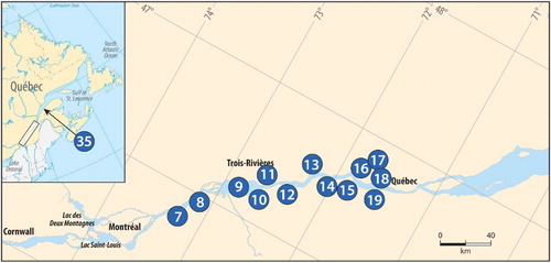
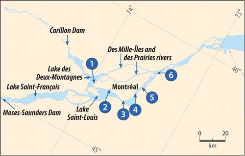
Fig. 2 Position of the water level gauges, flow sections, and meteorological stations in the downstream portion of the model domain.

Fig. 3 Position of the water level gauges around the Montréal Islands.

a Bathymetry

The bathymetry used to characterize and update each section of the model comes from Canadian Hydrographic Service surveys. Bathymetry was provided in local Chart Datum reference and was converted to common International Great Lakes Datum (NOAA, 2013) vertical reference for continuity in the model.

b Water Level

Water level observations were used to force the model at the downstream boundary as well as for calibration and validation throughout the domain. They are provided at 3-minute intervals by the Canadian Hydrographic Service at the specific water level gauges considered here (Appendix, Table A2). Water levels from Environment Canada, Water Office (http://wateroffice.ec.gc.ca/; stations 1 to 3) are provided at 15-minute intervals and were interpolated to 3-minute intervals in the model.

c Wind

Wind data were used to derive the effects of storm surges on the water levels between Orléans Island and the downstream boundary. This forcing was included as an additional contribution to the water levels at the model boundary. Winds are provided at 3-hour intervals by Environment Canada (http://weather.gc.ca/) for Québec City Jean Lesage International Airport (Station 22), Saint-François (Station 28), and Îles-aux-Grues (Station 32).

d St. Lawrence River Section Flow

Simultaneous water levels and currents were measured by Matte et al. (2014a), using a real-time kinematic (RTK) global positioning system (GPS) and an Acoustic Doppler Current Profiler (ADCP), respectively, and reinterpolated at 2-minute intervals along 13 cross-sections of the St. Lawrence River (Figs 1 and 2, and listed in Table A3 of the Appendix). They were converted to flow data and the uncertainties associated with these estimates were computed (Table A3 in the Appendix). These flow data were used to further validate model results.

e Upstream and Tributary Flow

The outflow from Lake Ontario is the main contributor to the St. Lawrence River. The flow from electricity production at Moses-Saunders Dam in Cornwall, Ontario, was calibrated using simultaneous observation of currents. According to Environment Canada the uncertainty associated with the published flow is 5% (R. Caldwell, personal communication, 2010). The second major contributor is the Ottawa River. Its flow was estimated by electricity production at Carillon Dam (Hydro-Québec). The uncertainty associated with this flow is not as well documented but is expected to be larger. Minor contributions are made by other tributaries to the St. Lawrence River. The model uses the flows from L'Assomption (NS near Station 6), Yamaska (SS near Station 8), Richelieu (SS near Station 8), Saint-François (SS near Station 8), Nicolet (SS near Station 8), Maskinongé (NS near Station 9), St-Maurice (NS near Station 11), Noire (SS near Station 11), Bécancour (SS near Station 12), Batiscan (NS near Station 13), Portneuf (NS near Station 17), Jacques-Cartier (NS near Station 19), Chaudière (SS near Station 20), and Saint-Charles (NS near Station 21), where NS and SS refer to the North and South Shores of the St. Lawrence River, respectively. These flows are, for the most part, evaluated from stage-discharge relationships established by the government of Québec (Centre d’expertise hydrique du Québec, Ministère du Développement durable, Environnment et Lutte contre les changements climatiques; https://www.cehq.gouv.qc.ca/), and their uncertainties are well documented. The other flow data come from Hydro-Québec and are estimated using similar types of measurements (Richelieu, Saint-François, and St-Maurice rivers). Tributary flows are multiplied by a factor specific to each river to include the drainage basin not covered by the river gauge (Morse, 1991). Flow data are provided as daily values and were interpolated at 3-minute intervals for use in the model.

3 Methods

a The Hydrodynamic Model Domain and Discretization

The previous version of the hydrodynamic model was documented by Lefaivre et al. (2009). It is a one-dimensional model initially developed by Gunaratnam and Perkins (1970) and others (Dailey & Harleman, 1972; Wood, Harley, & Perkins, 1972). Morse (1991) applied the model to the St. Lawrence River. The model solves the St. Venant equations for unsteady flow. The Coriolis force is neglected; the pressure is considered hydrostatic (no vertical acceleration), and the water density is considered uniform.

The St. Lawrence River is modelled from Montréal (Station 4) to Saint-Joseph-de-la-Rive (Station 34). Several improvements were made in this new implementation of the model. In the previous version, the downstream boundary was located at Québec, which made the operation awkward because the mean water level was influenced by the flow from the upstream boundary. The model downstream boundary was, therefore, extended to Saint-Joseph-de-la-Rive (Station 34) in order to remove this dependence on the upstream flow and to improve the water level forecast. This change of boundary also allowed inclusion of an area of recurrent dredging activity downstream of Québec, known as Traverse du Nord, running south and east of Orléans Island between 11 km southwest of Saint-François (Station 28) to Rocher Neptune (Station 31). As a result, water level forecasts from the operational model are used as an integrity system to support monitoring of dredging activities in the river by the Canadian Hydrographic Service, in parallel with their main GPS system.

The St. Lawrence River discharges into the Gulf of St. Lawrence and outflows into the Atlantic Ocean. A non-tidal, unidirectional flow regime is observed at Montréal down to Trois-Rivières where tides start modulating the flow. Flow reversal from the action of tides is observed at Batiscan (Station 13) and seaward, increasing in duration down to Saint-Joseph-de-la-Rive (Station 34), where the ebb and flood discharges are almost symmetrical. With these flow conditions it is natural to operate the model with flow boundary conditions upstream and water levels downstream. This set-up also provides better numerical stability in the operation of the model than water levels at both boundaries. However, the quality of the two datasets is known to be highly variable. Although the water level is accurately known at stations in the domain, flow data quality is variable. The implication for the model operation is described in Section 3b.

The downstream boundary conditions are now set by tidal predictions and atmospheric influence only. This extended section is wide, thus partitioning it into three channels is justified — North, Middle, and South — each one with its own boundary (shown as N, M, and S, respectively, in Fig. 2, with the sections of the model delineated by black lines). The three channels converge into two, north and south of Orléans Island. The domain is also partly in salt water in the last 30 km. It is in well-mixed conditions for 20 km and stratified only in the last 10 km, with salinity varying from 10 to 20 (Painchaud, Lefaivre, Therriault, & Legendre, 1995). The density influence at the boundary was taken into account in the calibration process as described below.

The number of sections (reaches) was increased from 26 to 208, and the number of steps per reach was increased to 10 everywhere. The bathymetry of all model sections, as well as their vertical elevation values, was updated to the common vertical reference, the International Great Lakes Datum — 1985 (NOAA, 2013). The model computes water level and flow at the reaches using a finite element scheme, then interpolates between reaches over the 10 steps using a finite difference scheme. The output results are now given for 1061 steps along the main navigational channel (compared with 433 previously), with parallel sections in some areas but mainly in the downstream part of the domain, hence its name STLT1061, for ST. LaurenT 1061step river model.

b Open Boundary Conditions

1 Upstream flow

As shown in Fig. 3, the upstream inflow to the model comes from a variety of rivers but feeds only two lakes: Lake des Deux-Montagnes and Lake Saint-Louis. The major contributor to Lake des Deux-Montagnes is the Ottawa River with a much smaller contribution from the Du Nord River on its north shore. Lake Saint-Louis receives part of the outflow from Lake des Deux-Montagnes as well as the Chateauguay River on its south shore and the outflow of Lake Saint-François. The latter is mainly fed by the outflow from Lake Ontario but also from the Grass, Raquette, St. Regis, and Salmon rivers from the Adirondack basin in the United States. Instead of monitoring the flows of all these rivers, a simpler way of assessing the flows at the upstream boundary was used for the hindcast. From the water level observed at Sainte-Anne-de-Bellevue (Station 1) for Lake des Deux-Montagnes and at Pointe-Claire (Station 2) for Lake Saint-Louis, outflows were estimated using stage-discharge relationships. Lake des-Deux-Montagnes outflows through four channels, as shown in Fig. 3. The two north ones feed des Milles-Îles and des Prairies rivers flowing on the north side of Montréal Island and the two south ones flow into Lake Saint-Louis. Stage-discharge relationships for these channels were calibrated by Environment Canada (J.F. Cantin, personal communication, 2009). The outflow of Lake Saint-Louis is known at Lasalle (Station 3), from the Water Office, Environment Canada. However, we chose to use the observations at Pointe-Claire (Station 2) and estimate the stage-discharge relationship that best reproduces downstream water levels in the model. Pointe-Claire (Station 2) water levels, which do not share common vertical datum with Lasalle (Station 3), were used to validate the incoming flows in forecast mode. In this mode, incoming flows to Lake des Deux-Montagnes and Lake Saint-Louis are computed with the assimilation of water levels recorded at Sainte-Anne-de-Bellevue (Station 1) and Pointe-Claire (Station 2) over time with the above stage-discharge relationships.

In this study, we compared the two outflow evaluations of Lake Saint-Louis, the one based on the Pointe-Claire (Station 2) gauge and the published one at Lasalle (Station 3). A first estimate of the stage-discharge relationship with the Pointe-Claire water levels was calculated using available data (i.e., the monthly flow values at Québec from Bourgault and Koutitonsky (1999)), the river flows from Lake des Deux-Montagnes and the tributary rivers listed above. To validate this crude relationship, the water level at Varennes (Station 6) was used as a reference because it is where Lake des Deux-Montagnes discharges through des Milles-Îles and des Prairies rivers into the St. Lawrence River. The flow from Lake Saint-Louis as input to the model was varied until the model results at Varennes reproduced the water level observations. The resulting stage-discharge relationship is shown in Fig. 4 over the period. The equation for the regression line is:(1) where F is the flow transport in cubic metres per second at the upstream boundary of the model and η the water level in metres at the Pointe-Claire station.

Fig. 4 Stage-discharge relationship at Pointe-Claire (Station 2) for the model upstream flow boundary conditions.

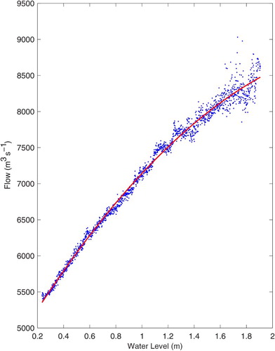
The water level is referenced to the local Chart Datum at Pointe-Claire as posted by the Water Office, Environment Canada. The standard deviation of the data around this regression line is small, 92 m³ s⁻¹. This result represents the flow as seen by the model that best reproduces the water levels. The flow is close to the ones posted for Lasalle (Station 3) but 4.3% less, on average, over the 2005–2012 period.

2 Downstream water level

Water levels are specified at the three downstream boundaries shown in Fig. 2 as N, M, and S for the North, Middle, and South channels, respectively. For the northern boundary, the water level observations at the nearby Saint-Joseph-de-la-Rive station are available. Tidal harmonic constituents are evaluated for this station using one-year tidal analyses (Foreman, 1978) and vector averages (Crawford, 1982) computed over the 1994–2009 period (A. Godin, personal communication, 2014). For the middle and southern boundaries, hourly water level values were obtained from the results of a three-dimensional model of the region (Saucier et al., 1999). Tidal analysis (Foreman, 1978) of the water levels at the grid points of the model provided the needed tidal harmonic constituents.

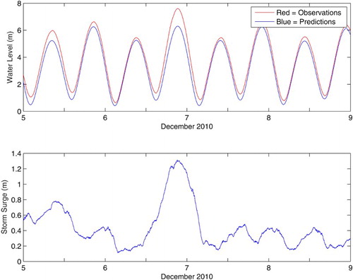
The next task was to identify the non-tidal part of the observed data at the northern boundary in order to be able to add it to the tidal reproduction at the middle and southern boundaries. These residual water levels can be illustrated on two temporal scales. First, at an hourly time scale, non-tidal variations associated with storm surges were identified, as shown in Fig. 5 for the December 2010 storm surge. The difference between predicted and observed water levels at the downstream station of Saint-Joseph-de-la-Rive (Station 34) is added to the time series of water levels at the two other boundaries, M and S, shown in Fig. 2.

Fig. 5 Example of a storm surge observed at the Saint-Joseph-de-la-Rive (Station 34) water level gauge.

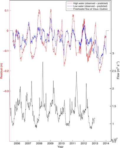
Second, interannual variability is observed at a monthly time scale, with strong differences between the high and low water level marks, as shown in Fig. 6. A 30-day moving average filter was applied to both series in Fig. 6 to illustrate this low-frequency and low-amplitude oscillation. An annual cycle dominates the high water time series, whereas semi-annual fluctuations are observed in the low water time series. To verify whether these variations are synchronized with the annual runoff cycle, the freshwater flow at Québec, as reconstructed below, is also shown in Fig. 6. Although part of these oscillations may be associated with unresolved low-frequency tides or river discharge, their correlation with the freshwater runoff is not obvious. Rather, they are most likely non-local in origin and the result of atmospheric forcing on the waters of the east coast of Canada. In fact, this area of the St. Lawrence River is known to intensify the amplitude of storm surges because of the shallowing of the bathymetry as well as the funnelling of the coastline topography. The low-frequency oscillations also appear to be amplified when compared with Rimouski (Station 35) tidal data, where such oscillations are absent. The discrepancy between high and low water may be further explained by wave propagation differences with the water depth difference between high and low tide. Interpolation between successive high and low water values is done using cubic splines to obtain a 3-minute time series of the low-frequency oscillations.

Fig. 6 Low-frequency oscillations at High Water and Low Water marks observed at Saint-Joseph-de-la-Rive water level gauge with a 30-day moving average filter on the residual (observations minus tidal predictions). The bottom curve is the daily average flow at the Vieux-Québec section (Station 21).

In summary, the boundary conditions for the middle and southern boundaries are the sum of three components: the water levels from tidal harmonics extracted from a three-dimensional model, the low-frequency oscillation interpolated from the high and low water residuals, and the storm surges; the latter two from the observations at Saint-Joseph-de-la-Rive (Station 35). Calculating the low-frequency oscillation makes possible its use in the forecast operation of the model.

c Model Calibration for Water Levels

The model was operated using a 3-minute time step for the entire 2005–2012 period. Model calibration was performed using observations at water level stations (Table A2 in Appendix), which consisted of the following adjustments. For the unidirectional flow regime section from Montréal to Batiscan (Stations 4 to 13), the first criterion is the reproduction of the average water level. The width and depth of the sections and the bottom friction were adjusted to reproduce the observed levels at the stations. Integration of the bathymetric sections into the model discretized and linearized the navigational channel. The actual coastline is more complex than is captured by the model sections because the mean distance between bathymetric sections is relatively large (3 km). Thus, local adjustments to the width and depth of the sections were made so that the model results mimic observations. Bottom friction adjustments were based on a Manning coefficient that takes into account the nature of the substrate roughness, which varies from rocky, to sand waves, to silt. Then, the average error in water level was calculated at each station (model result minus observation). These differences were linearly interpolated between stations and used to correct the model outputs by subtracting them from the model results. Once the average water levels had been adjusted, the second criterion was applied to reproduce water level fluctuations as described below.

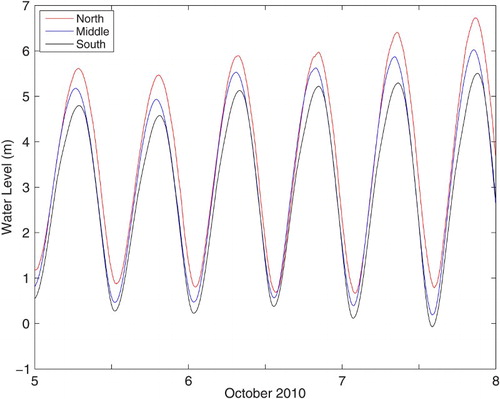
For the downstream section (Stations 14 to 34), the first criterion is also to reproduce the mean water level using the procedure described above. The second criterion is reproduction of high tide and low tide levels with the correct phase or timing. To reduce the errors between model results and observations, water level differences were calculated over a 29-day tidal cycle at every station in the area: Stations 21, 23, 25, 28, 29, 30, 31, 32, and 33. These differences were then subtracted from the boundary condition at one of the three downstream branches that corresponds to the section where the station is located. The difference is added over the whole period, keyed to the spring-neap cycle. For instance, for the northern section, the negative difference between the model results and the observations at Lauzon (Station 23) was added to the water level from the tidal harmonics at the boundary of section N. Tidal analysis is applied to this new water level time series to generate a new set of tidal constituents at the boundary. This iteration was carried out for the other stations under the influence of the boundary until an optimal result was obtained. The northern section includes water level observations at Rocher Neptune (Station 31), Banc-Cap-Brûlé (Station 29), and St-Laurent (Station 25) as well as the permanent gauge at Saint-François (Station 28) and those further upstream. For the middle section, data from Île-aux-Grues (Station 32) and Grosse-Île (Station 30) were used. For the southern section, data from Saint-Jean-Port-Joli (Station 33) were not available during the period considered, but previously recorded data from 1974 were used with hindcasts of the model over the same period. Typical water level results show differences in amplitude and phase between the three downstream boundaries as shown in Fig. 7. This optimization for tidal extrema induces a non-zero value in mean water level for the downstream stations.

Fig. 7 Example of the water levels at the three downstream boundaries. The difference in amplitude and phase among the three is the result of the calibration process using the observed water levels at the tidal gauges upstream of the boundaries.

A third effect that had to be taken into consideration was the wind stress within the model domain over the area between Orléans Island and the downstream boundaries. As shown in Fig. 2, this area is a large body of water where wind fetch is appreciable. Wind recorded at Saint-François (Station 28) was used when available, with data from Québec City Jean Lesage International Airport (Station 22) and Île-aux-Grues (Station 32) filling the gaps when necessary. Wind intensity was evaluated in the northeast–southwest direction. Equation (2) was used to calculate the positive storm surge water level induced by wind intensity from the northeast (W_NE has a positive value), and Eq. (3) was used to calculate the negative storm surge induced by wind intensity from the southwest (W_SW has a negative value),(2) (3) where η is the water level in centimetres to be added to the downstream boundary values at N, M, and S, and W_NE and W_SW are the northeast and the southwest components of the wind intensity in kilomteres per hour.

The relations in Eq. (2) and Eq. (3) are not symmetric because it is easier to reduce the outflow from the St. Lawrence River with the wind stress than to increase its outflow because of the action of the bottom friction. This set of equations was calibrated with storm surges observed at Lauzon (Station 23) and with wind in the area of Rimouski (Station 35). The storm surges were evaluated from the observed water levels minus the tidal harmonic time series, generated using long-term tidal analysis, as shown in Fig. 5. The resulting value for water level was added to the boundary conditions of all three downstream branches, N, M, and S, shown in Fig. 2. Using this wind influence, the modelled water levels were closer to the observations than without it, and the standard deviation of the error was reduced.

The mean error and standard deviation at each station over the hindcast period is shown in Fig. 8.

Fig. 8 Mean error, standard deviation, and γ² value of the model results for each tidal station. The tidal gauge number refers to the consecutive numbers in Table A2.

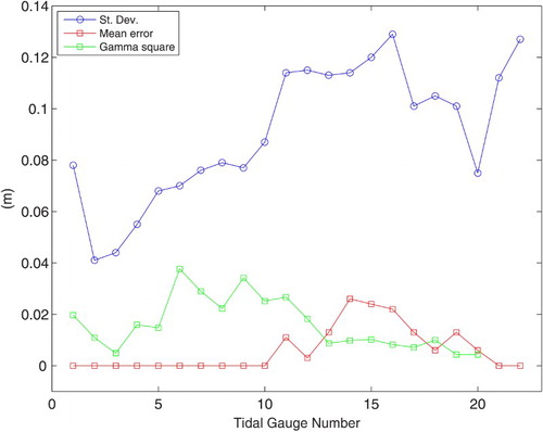
One measure of the performance of the model is γ². It is calculated using Eq. (4) and is dimensionless (Thompson et al., 2003).(4)

The observations and model results used in the evaluation are at 3-minute intervals over the 2005–2012 period at the stations.

The value of γ² is lower than 0.04 over the domain. It is lowest at the downstream end, less than 0.01, where the tidal range is the largest. The mean error is small, 26 mm at most. On the other hand, the standard deviation of the error increases from the upstream to the downstream part of the domain where tides are large. However, analysis of the model results showed that phase differences of the tidal progression between model results and observations through the domain are as important as the difference in amplitudes. To illustrate this fact, an analysis of the actual water level values from the model results at high and low water compared better with observations (Fig. 9). The standard deviation of the amplitude error at high and low water remains below 10 cm for most stations.

Fig. 9 Standard deviation of the model result errors at the downstream tidal stations. The tidal gauge number refers to the consecutive number of Table A2.

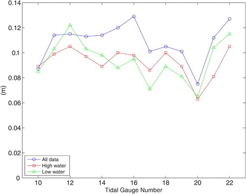
The mean error over the domain is 0.6 cm with values from zero in the upstream section to a maximum value of 2.6 cm at Québec’s Bridge, Station 20 (Table A2). The mean standard deviation is 11 cm with individual stations up to 13 cm at the downstream end of the domain. The main difference between the model results and the observation is not so much the value of high and low water but rather the time at which they occur in the model compared with the observation. The difference in time, hence, the timing of the tidal extrema in the model is primarily responsible for higher values in the standard deviation of the error. If one calculates the difference in amplitude, the mean standard deviation of the error at high and low water values is lower, at 9 cm as shown in Fig. 9.

d Model Validation for Flow

Comparison of flows derived from ADCP measurements (Matte et al., 2014a) with flows from the model for the same sections and times is shown in Fig. 10 for Vieux-Québec section (Station 21). Because the observed flows are at 2-minute intervals and the modelled flows are at 3-minute intervals, the comparison was done at 6-minute intervals. The flows were normalized to the maximum value of the observed flow. The model results underestimate the flows, as shown by the ratio. The mean ratio values are shown in Table 1 for all sections. For a given section, the individual ratios were not used in the computation of the mean ratio when the instantaneous flow was less than 20% of the maximum value for that section. Overall, the ratios are highly consistent throughout the domain except for section 27 (Île d’Orléans-North; Table A3). The water level was not calibrated in the present model for that section and the ratio should not be considered. When this section value is excluded, the mean ratio is 0.86 with a standard deviation of 0.02 (Table 1). The small variations in the ratio are not correlated with the spring-neap tidal cycle or with the distance from Trois-Rivières to Orléans Island. A mean ratio of 0.86 indicates that the volume of water in the model is less than that in the field. It is the result of the model adjustments to a given set of friction and bathymetry that provides a good representation of the water level and of flows, given that the latter are corrected by a constant factor.

Fig. 10 Flows at the Vieux-Québec section (Station 21) derived from current measurements and from the model results, along with the ratio between the two values. The time on the abscissa is hours from 14:48 utc on 15 June 2009.

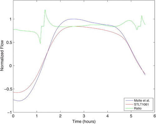
Table 1. The ratio of the model flow results to flows derived from ADCP measurements for the sections. Mean and standard deviation values are calculated excluding Station 27.

Station Number	Section	Mean Ratio
11	Trois-Rivières	0.84
12	Bécancour	0.87
13	Batiscan	0.85
15	Grondines	0.85
16	Deschambault	0.86
17	Portneuf	0.87
18	Neuville	0.87
19	Saint-Nicolas	0.82
21	Vieux-Québec	0.84
23	Lauzon	0.92
24	Beauport	0.86
26	Orléans Island South	0.89
27	Orléans Island North	0.63
	Mean value (without Station 27)	0.86
	St. Dev. (without Station 27)	0.02

The 14% difference between the model results and the derived flows exceeds the 4.7% error estimates at Vieux-Québec, as shown in Table A3 (Appendix). Using this calibration, for example, to reconstruct the flows for the 2005–2012 period at Vieux-Québec section (Section 4.b), the model results at 3-minute intervals were increased by 1/0.86, then averaged using a low-pass filter (moving average over, respectively, 24, 24, and 25 hours, (Godin, 1972) and sampled at noon (utc) every day to obtain a daily average value. Using the same method, the flows can be computed for all stations and sections in the model.

4 Results and discussion

a Water Levels and Wind Forcings

The uncertainties associated with the water level model results were documented in Section 3.c. The hindcast process highlights the influence of local winds on water levels in the downstream part of the domain and the ability of the model to take this effect into account through its boundary condition. The formulation of its influence is rather crude, using wind intensity instead of wind stress. This part remains to be updated. Nevertheless, it clearly shows that storm surges are not solely a result of downstream conditions and that local winds within the model domain are also important. At the downstream boundary of the model, we will use for the operational water level daily forecasts (Lefaivre et al., 2009) the upcoming storm surge forecasts to be issued from a global model (Xu, Savard, & Lefaivre, 2015), but the present analysis shows that the local wind effects within the domain need to be taken into account.

b St. Lawrence River Flows

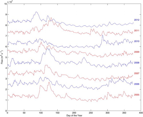
The hindcast daily flow values of the St. Lawrence River at Vieux-Québec section (Station 21) are shown for the 2005–2012 period in Fig. 11. They also appear at the bottom of Fig. 6 as a continuous series. In Fig. 11, the large interannual variability of the flow is clear. Spring freshet is known to vary in amplitude and timing. For instance, 2010 stands out with a very small spring freshet and a larger flow in the fall. The 2012 freshet occurred as early as 23 March, but in 2011 it was as late as 6 May. Interannual variability is also observed in the flow intensity in the fall. For instance, the 2006 broad maximum of 18,000 m³s⁻¹ is well above the mean value of 11,000 m³s⁻¹ of the other years.

Fig. 11 Daily flow values at the Vieux-Québec section (Station 21) for the years of the hindcast period 2005–2012. The flow on the ordinate is for 2005 data; 10,000 m³ s⁻¹ has been added consecutively to each following year for clarity.

Another way to confirm the calibration of the flows is to consider the time series of the flow calculated by the model at Vieux-Québec section (Station 21) using the monthly values posted on the St. Lawrence Global Observatory website using the relationship reported in Bourgault and Koutitonsky (1999). The model results shown in Fig. 12 are averaged over each month, and for this comparison the hindcast period is extended to cover the years 1980 to 2012. The regression between the two results is shown in Fig. 12 and in Eq. (5):(5) where F_B&K is the monthly flow transport from Bourgault and Koutitonsky (1999), and F_Model is the monthly flow transport from the results of the present model.

Fig. 12 Regression between the monthly-mean flows from the present model results with the monthly-mean flows using the Bourgault and Koutitonsky (1999) relationship.

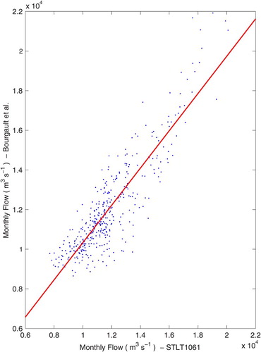
The slope of the regression is near one, a 6% difference, with an R² value of 0.78 and a standard deviation of the data around this regression line of 1200 m³ s⁻¹. The two methods are derived from two different models with different validation processes but converge toward the same mean results with some dispersion around the mean as shown by the value of R². The discrepancies come from the difference in the methods used. Bourgault and Koutitonsky (1999) used a one-dimensional model calibrated with ADCP measurements carried out on a section located between Québec’s Bridge (Station 20) and Vieux-Québec (Station 21). Afterwards, they compared the results of their model with the mean monthly water level at Neuville (Station 18). The correlation between the modelled flows and the water level observed at Neuville was satisfactory, so the mean monthly water level at Neuville was used as a proxy for the mean monthly flow. However, with Neuville’s water level as a proxy, incoming storm surges induce changes in water level that are interpreted as changes in the flow. These effects could be partly responsible for the dispersion observed in their results. The present model results include the storm surge effects explicitly which should produce more realistic flows and at a higher temporal resolution.

Comparison of the St. Lawrence River flows can also be done with another estimate of the St. Lawrence flow made by Bouchard and Morin (2000) and updated by Cantin, Bouchard, Morin, de Lafontaine, and Mingelbier (2006). They accounted for the contributions of all river tributaries to the St. Lawrence River using river gauge data with prorated values for the ungauged part of the basins based on the drainage area as described by Morse (1991).

The regression relation of daily flows between Bouchard and Morin (2000) and this study (Fig. 13) is given in Eq. (6) with an R² of 0.88. The comparison is good because the slope value is near one. However, the ordinate value of 450 at the origin is large and worth investigating.(6) where F_TS is the flow transport calculated in this study, and F_B&M is the flow transport calculated by Bouchard and Morin (2000).

Fig. 13 Regression of daily flows between Bouchard and Morin (2000), based on upstream flows, and this study.

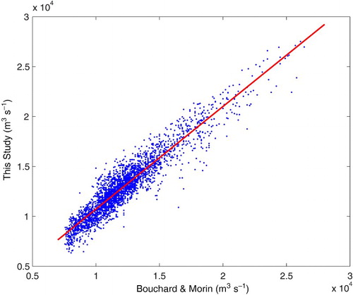
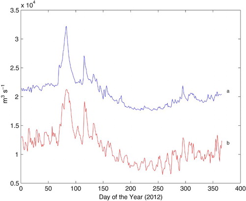
Looking closely at both flows (e.g., 2012 in Fig. 14), winter flows are systematically higher in this study than those of Bouchard and Morin (2000). If the winter months (January, February, and March) are removed from the analysis, then the regression relation improves as given in Eq. (7). The R² value is slightly better at 0.92; the slope value is still near one, but the main difference is that the value of the ordinate at the origin now 94, which is quite acceptable. Overall, during the winter months, the flows presented here over the 2005–2012 period are 11% higher than in the analysis of Bouchard and Morin (2000). We will work toward improving the flow values in winter in the future.(7)

Another difference between the two flow estimates appears at a fortnightly period. The St. Lawrence River flow is modulated by spring-neap variations of the tides at the Vieux-Québec station. These fluctuations are clearly reproduced in this study, which they are not in the analysis of Bouchard and Morin (2000). This modulation is needed to drive ecosystem models correctly.

Fig. 14 Estimated flows from Bouchard and Morin (2000) for 2012 in a and this study in b; 10,000 m³ s⁻¹ has been added to the former for clarity.

5 Summary

Recent changes in the operational one-dimensional model of the St. Lawrence River have been documented. The model was extended downstream to incorporate the estuarine transition zone between Orléans Island and Saint-Joseph-de-la-Rive, now represented by three separate branches. Forcing at the downstream boundaries includes a set of tidal predictions and atmospheric contributions. The number of sections has also been increased, yielding outputs of water levels and flows at 1061 steps along the river.

Calibration and validation of the model were carried out for water levels and flows, based on recently acquired data. The model performance was evaluated based on its capacity to reproduce mean water levels, tidal fluctuations and timing, wind-induced variations in water levels, and residual and tidal flows. Overall, model accuracy in water levels is good, with standard deviations lower than 13 cm at all stations. The model reproduces the flows with a systematic bias of 14% but is consistent throughout the domain.

Water level and daily flow hindcasts were produced for the 2005–2012 period and were analyzed for the Vieux-Québec station. The reconstructed flows are comparable to previous estimation methods used for the St. Lawrence River but with the added advantages of explicitly including storm surge effects, reproducing spring-neap variations of the flow, and outputting the results at 3-minute time intervals, similar to water level observations. Operational forecasts of water levels and flows are now available throughout the system with sufficient accuracy to be used in a variety of applications, including coastal flooding forecasts and hydrodynamic studies.

Acknowledgements

The two first authors were affiliated with the Canadian Hydrographic Service (CHS), Québec Region, when this study was initiated. We would like to acknowledge the support of the management team, in particular of former director Dr. Andrée Bolduc, for her steadfast support throughout this endeavour. Many other members of CHS made important contributions for which we are grateful: Annie Biron implemented the bathymetric sections in the model from the surveys; Frédéric Lavoie computed volumes from bathymetry over sections of the model; André Godin performed tidal analysis on water level data. The St. Lawrence Global Observatory management team gave us strong support, and Johanne Noël produced Figs 1, 2, and 3. Jean-François Cantin (Hydrologic and Ecohydraulics Division, Meteorological Service of Canada, Environment Canada) provided the stage-discharge relationships at the outflow of lakes des Deux-Montagnes and Saint-Louis as well as the water level data. We also wish to thank two anonymous reviewers for their constructive comments on a previous version of the manuscript.

Disclosure statement

No potential conflict of interest was reported by the authors.

Appendix

Table A1. Geographical positions of the stations with observations of water level (WL), current (C), flow (F), and wind (W).

Station Number	Station Name	Latitude (°North)	Longitude (°West)	Qualifier
1	Sainte-Anne-de-Bellevue	45.405	−73.956	WL
2	Pointe-Claire	45.428	−73.821	WL
3	Lasalle	45.415	−73.623	WL, F
4	Montréal Harbour	45.503	−73.546	WL
5	Frontenac	45.528	−73.540	WL
6	Varennes	45.685	−73.454	WL
7	Contrecoeur	45.836	−73.288	WL
8	Sorel	46.054	−73.119	WL
9	Lake St-Pierre	46.191	−72.894	WL
10	Port St-François	46.274	−72.621	WL
11	Trois-Rivières	46.335	−72.531	WL, C
12	Bécancour	46.410	−72.386	WL, C
13	Batiscan	46.497	−72.232	WL, C
14	Deschaillons	46.565	−72.106	WL
15	Grondines	46.575	−72.031	C
16	Deschambault	46.652	−71.907	C
17	Portneuf	46.678	−71.875	WL, C
18	Neuville	46.680	−71.563	WL, C
19	St-Nicolas	46.723	−71.382	C
20	Québec's Bridge	46.746	−71.287	WL
21	Vieux-Québec	46.811	−71.195	WL, C
22	Québec City Jean Lesage International Airport	46.800	−71.349	W
23	Lauzon	46.842	−71.164	WL, C
24	Beauport	46.855	−71.154	C
25	St-Laurent	46.854	−71.002	WL
26	Orléans I. South	46.904	−70.886	C
27	Orléans I. North	46.958	−71.012	C
28	Saint-François	46.994	−70.802	WL, W
29	Banc-Cap-Brûlé	47.093	−70.717	WL
30	Grosse-Île	47.020	−70.671	WL
31	Rocher Neptune	47.174	−70.639	WL
32	Île-aux-Grues	47.055	−70.532	WL,W
33	Saint-Jean-Port-Joli	47.216	−70.275	WL
34	St-Joseph-de-la-Rive	47.437	−70.363	WL
35	Rimouski	48.480	−68.510	WL

Table A2. List of water level stations and length of the water level time series. The Consecutive Number is the number used in Figs 8 and 9.

Consecutive Number	Station Number	Water Level Gauge	Years
	1	Sainte-Anne-de-Bellevue	2005–2013
	2	Pointe-Claire	2005–2013
	3	Lasalle	2005–2013
1	4	Montréal Harbour	2005–2013
2	5	Frontenac	2005–2013
3	6	Varennes	2005–2013
4	7	Contrecoeur	2005–2013
5	8	Sorel	2005–2013
6	9	Lake St-Pierre	2005–2013
7	10	Port St-François	2005–2013
8	11	Trois-Rivières	2005–2013
9	12	Bécancour	2005–2013
10	13	Batiscan	2005–2013
11	14	Deschaillons	2005–2013
12	17	Portneuf	2005–2013
13	18	Neuville	2005–2013
14	20	Québec's Bridge	Summer 2012
15	21	Vieux-Québec	2012–2013
16	23	Lauzon	2005–2012
17	25	Saint-Laurent	Summer 2012
18	28	Saint-François	2005–2013
19	29	Banc-Cap-Brûlé	Summers 2005–2013
21	30	Grosse-Île	Summer 2010
20	31	Rocher Neptune	Summers 2005–2013
22	32	Île-aux-Grues	Summer 2010
	33	Saint-Jean-Port-Joli	1974
	34	St-Joseph-de-la-Rive	2005–2013
	35	Rimouski	2005–2013

Table A3. List of the sections with current measurements.

Station Number	Section	Date	Observation (Hours)	Error in the Flow (%)
11	Trois-Rivières	18 June 2009	0.8	1.7
12	Bécancour	18 June 2009	5.0	2.1
13	Batiscan	23 June 2009	7.6	7.3
15	Grondines	19 June 2009	8.9	1.8
16	Deschambault	20 August 2009	10.1	6.3
17	Portneuf	26 June 2009	6.7	4.5
18	Neuville	25 June 2009	9.1	2.3
19	Saint-Nicolas	21 August 2009	8.8	2.2
21	Vieux-Québec	15 June 2009	11.3	4.7
23	Lauzon	24 June 2009	11.4	3.1
24	Beauport	24 June 2009	10.7	14.7
26	Orléans I. South	24 August 2009	7.6	2.1
27	Orléans I. North	25 August 2009	8.7	5.4

References

- Bouchard, A., & Morin, J. (2000). Reconstitution des débits du fleuve Saint-Laurent entre 1932 et 1998. Rapport Technique RT-101, Environnement Canada, Sainte-Foy.
- Bourgault, D., & Koutitonsky, V. G. (1999). Real-time monitoring of the freshwater discharge at the head of the St. Lawrence Estuary. Atmosphere-Ocean, 37, 203–220. doi: 10.1080/07055900.1999.9649626
- Cantin, J.-F., Bouchard, A., Morin, J., de Lafontaine, Y., & Mingelbier, M. (2006). Anthropogenic modifications and hydrological regime in the fluvial portion of the St. Lawrence downstream from Cornwall. In A. Talbot (Ed.), Water availability issues for the St. Lawrence River – An environmental synthesis (pp. 13–24). Montréal: Environment Canada.
- Crawford, W. R. (1982). Analysis of fortnightly and monthly tides. Inteternational Hydrographic Review, 59(1), 131–141.
- Dailey, J. E., & Harleman, D. R. F. (1972). Numerical model for the prediction of transient water quality in estuary networks. Cambridge, Mass.: Hydrodynamics Laboratory, Massachusetts Institute of Technology, Report No. 158, RT72–72.
- Foreman, M. G. G. (1978). Manual for tidal currents analysis and prediction. Pacific Marine Science Report 78–6. Sidney, BC: Institute of Ocean Sciences, Patricia Bay.
- Godin, G. (1972). The analysis of tides. Toronto, Canada: University of Toronto Press.
- Gunaratnam, D. J., & Perkins, F. E. (1970). Numerical solutions for unsteady flows in open channels. Cambridge, Mass.: Hydrodynamics Laboratory, Massachussetts Institute of Technology, Report No. 127, July 1970.
- Lefaivre, D., Hamdi, S., & Morse, B. (2009). Statistical analysis of the 30-day water level forecasts in the St. Lawrence River. Marine Geodesy, 32(1), 30–41. doi: 10.1080/01490410802661971
- Matte, P., Secretan, Y., & Morin, J. (2014a). Quantifying lateral and intratidal variability in water level and velocity in a tide-dominated river using combined RTK GPS and ADCP measurements. Limnology and Oceanography Methods. 12, 279–300.
- Matte, P., Secretan, Y., & Morin, J. (2014b). Temporal and spatial variability of tidal-fluvial dynamics in the St. Lawrence fluvial estuary: An application of nonstationary tidal harmonic analysis. Journal of Geophysical Research: Oceans, 119, 5724–5744. doi:10.1002/2014JC009791
- Morse, B. (1991). Mathematical modelling of sediment transport and bed-transients in multi-channel river networks under conditions of unsteady flow (Ph.D. thesis). Department of Civil Engineering, University of Ottawa, Ottawa, Ont.
- NOAA. (2013). Great Lakes, establishment of international Great Lakes Datum, 1985. Silver Spring, Maryland: National Oceanic and Atmospheric Administration.
- Painchaud, J., Lefaivre, D., Therriault, J.-C., & Legendre, L. (1995). Physical processes controlling bacterial distribution and variability in the upper St. Lawrence Estuary. Estuaries, 18, 434–444. doi: 10.2307/1352362
- Saucier, F.-J., Chassé, J., Couture, M., D’Astous, A., Dorais, R., Lefaivre, D., & Gosselin, A. (1999). The making of a surface current atlas of the St. Lawrence. In C. A. Brebbia & P. Anagnostopoulos (Eds.), WIT Transactions on the built environment, Vol. 43, pp. 87–97. Southampton, UK: WIT Press.
- Saucier, F. J., Roy, F., Senneville, S., Smith, G., Lefaivre, D., Zakardjian, B., & Dumais, J.-F. (2009). Modélisation de la circulation dans l'estuaire et le golfe du Saint-Laurent en réponse aux variations du débit d'eau douce et des vents. Revue des sciences de l'eau, 22(2), 159–176. doi: 10.7202/037480ar
- Smith, G. C., Roy, F., & Brasnett, B. (2013). Evaluation of an operational ice–ocean analysis and forecasting system for the Gulf of St Lawrence. Quarterly Journal of the Royal Meteorological Society, 139(671), 419–433. doi:10.1002/qj.1982
- Thompson, K.R., Sheng, J., Smith, P.C., & Cong, L. (2003). Prediction of surface currents and drifter trajectories on the inner Scotian Shelf. Journal of Geophysical Research, 108(19C9), 3287, doi:10.1029/2001JC001119
- Wood, E. F., Harley, B. M., & Perkins, F. E. (1972). Operational characteristics of a numerical solution for the simulation of open channel flow. Cambridge, Mass.: Hydrodynamics Laboratory, Massachusetts Institute of Technology, Report No. 150, RT72–30.
- Xu, Z., Savard, J.-P., & Lefaivre, D. (2015). Data-assimilative hindcast and climate forecast of storm surges with an ASGF regression model. Atmosphere-Ocean, 53(5), 464–475. doi:10.1080/07055900.2015.1079774