Hydrography and Coastal Circulation along the Halifax Line and the Connections with the Gulf of St. Lawrence

ABSTRACT

Acoustic Doppler Current Profilers and underwater gliders were simultaneously deployed as part of the Ocean Tracking Network to continuously monitor the Halifax Line (HL) and the Nova Scotia Current (NSC) between 2008 and 2014. The HL transects the Scotian Shelf, which connects dynamically important areas, such as the Grand Banks, the Gulf of Maine, and the Gulf of St. Lawrence (GSL). The oceanographic measurements made at the HL during this period provide a unique opportunity to study the temperature, salinity, and alongshore current conditions and variability at both seasonal and interannual time scales. The analysis of observations reveals that the water over the Scotian Shelf is mainly composed of water coming from the Gulf of St. Lawrence (Cabot Strait subsurface water) in the upper layer (30 to 50 m, 81%) and Warm Slope Water below 100 m (77%), highlighting the connectivity between the GSL and the Scotian Shelf. The temperature–salinity characteristics of the Cold Intermediate Layer (CIL) observed along the HL and located mainly between 50 and 100 m, is indistinguishably influenced by both water coming from the Inshore Branch of the Labrador Current and CIL water formed in the GSL. These proportions stay similar over interannual time scales, suggesting that the 2012 warm anomaly observed over the Scotian Shelf is primarily driven by the advection of already anomalously warm water coming from offshore regions. The analysis of glider data also reveals that most of the alongshore transport over the Scotian Shelf occurs within the first 60 km from the coast, where the NSC is located. It was found that the freshwater discharge from the St. Lawrence River at Québec and the alongshore transport across the NSC have a significant covariance at a 9-month lag. The Empirical Orthogonal Function (EOF) analysis demonstrates that most of the current variability (between 78 and 92%) can be explained by the first EOF, which represents the baroclinicity resulting from the freshwater outflow coming from the GSL. Part of the second EOF is associated with the local wind forcing and explains between 4 and 14% of the NSC variability.

RÉSUMÉ

[Traduit par la rédaction] Des profileurs de courant Doppler acoustiques et des planeurs sous-marins ont été déployés simultanément dans le cadre de l’Ocean Tracking Network afin de surveiller en continu la ligne d’Halifax et le courant de la Nouvelle-Écosse, entre 2008 et 2014. La ligne d’Halifax traverse le plateau néo-écossais, qui, lui, relie dynamiquement des zones importantes comme les Grands bancs, le golfe du Maine et le golfe du Saint-Laurent (GSL). Les mesures océanographiques relevées le long de la ligne d’Halifax au cours de cette période fournissent une occasion unique d’étudier la température, la salinité, le courant littoral et leur variabilité, à des échelles saisonnières et interannuelles. L’analyse d’observations révèle que les eaux de la couche supérieure au-dessus du plateau néo-écossais se composent principalement d’eau du GSL (eau de subsurface du détroit de Cabot, 30 à 50 m, 81 %) et d’eau chaude de la pente continentale sous 100 m (77 %), mettant ainsi au jour le lien entre le golfe du Saint-Laurent et le plateau néo-écossais. La température et la salinité de la couche intermédiaire froide, qui sont observées le long de la ligne d’Halifax, principalement entre 50 et 100 m, sont influencées à la fois et sans distinction par l’eau venant du bras côtier du courant du Labrador et par l’eau de la couche intermédiaire froide formée dans le golfe du Saint-Laurent. Ces proportions restent semblables aux échelles interannuelles, ce qui laisse penser que l’anomalie chaude de 2012 observée au-dessus du plateau néo-écossais est avant tout régie par l’advection des eaux déjà anormalement chaudes qui arrivent du large. L’analyse des données de planeur révèle aussi que la majeure partie du transport littoral au-dessus du plateau néo-écossais se produit à moins de 60 kilomètres de la côte, où se situe le courant de la Nouvelle-Écosse. Nous avons relevé que l’apport d’eau douce provenant du fleuve Saint-Laurent à Québec et le transport littoral traversant le courant de la Nouvelle-Écosse montrent une covariance significative (σ_xy = 0,37) pour un décalage de 9 mois. L’analyse des fonctions orthogonales empiriques démontre que la majeure partie de la variabilité du courant (entre 78 et 92 %) peut s’expliquer par la première fonction orthogonale, qui représente la baroclinicité que produit l’apport d’eau douce issue du golf du Saint-Laurent. Une partie de la seconde fonction orthogonale est associée au forçage du vent local et explique entre 4 et 14 % de la variabilité du courant de la Nouvelle-Écosse.

KEYWORDS:

• observations
• Scotian Shelf
• Nova Scotia Current
• Gulf of St. Lawrence
• St. Lawrence River
• Ocean Tracking Network

1 Introduction

Bounded by the Laurentian Channel to the east, the Northeast Channel to the west, and a continental slope to the south, the Scotian Shelf is dynamically connected to geographic areas such as the Grand Banks, the Gulf of Maine, and the Gulf of St. Lawrence (GSL). The seasonal mean circulation on the Scotian Shelf is characterized by a persistent southwestward coastally trapped current known as the Nova Scotia Current (NSC) and a southwestward alongslope current located at the shelf break (Loder, Han, Hannah, Greenberg, & Smith, 1997; Smith & Schwing, 1991). The latter originates from the offshore branch of the Labrador Current. The mesoscale structure of the flow on the Scotian Shelf is affected by the irregular topography composed of banks and basins, which are associated with anticyclonic and cyclonic circulation features, respectively (Han & Loder, 2003).

Previous studies demonstrated that the major physical processes affecting the circulation on the Scotian Shelf were both baroclinic (Smith & Schwing, 1991) and barotropic (Thompson & Sheng, 1997) over a broad range of time scales. Smith and Schwing (1991) found that the winter circulation measured along the Halifax Line (HL) agreed roughly with the geostrophic currents estimated from concurrent density transects, confirming that the buoyancy fluxes associated with the advection of the freshwater discharge from the St. Lawrence Estuary through the western GSL and Cabot Strait could be a major forcing mechanism for the NSC (Drinkwater, Petrie, & Sutcliffe, 1979).

Temporal variability in the circulation on the Scotian Shelf is significantly affected by the time-varying local surface wind stress, particularly in both the inertial (17–22 h) and synoptic (2–10 days) frequency bands, with a greater response in water columns shallower than 100 m (Schwing, 1989, 1992b). The temporal variability at lower frequencies in the subsurface pressure field and in the bottom temperature was found to correlate with travelling shelf waves generated by remote winds (Schwing, 1992a, 1992b) and large-scale meteorological forcing. The latter was found to affect the strength and hydrographic signature of the Labrador Current (Petrie, 2007).

Previous oceanographic programs conducted over the Scotian Shelf generally focused on sampling along the traditional HL, which is an across-shelf transect running from the coastal water off Halifax to the shelf break (Fig. 1). During winter 1985–86, for example, continuous current velocity and hydrographic measurements were made on the Scotian Shelf as part of the Canadian Atlantic Storm Program. Unfortunately, observations during this period were only collected at discrete depth levels and covered a short period of time (3 months; Anderson & Smith, 1989). As a result, the oceanographic observations made by this program were too short to be used in characterizing the seasonal, or interannual, variability of the ocean circulation and hydrography on the Scotian Shelf. Since 1998 the ongoing Atlantic Zone Monitoring Program (AZMP) has partially addressed this issue by measuring hydrographic variables twice a year, on average, along the HL (Therriault et al., 1998). However, the low temporal resolution of this program prevents a proper study of the seasonal cycle and introduces issues when looking at the interannual variability because the data can suffer from significant aliasing (Mann, 1969; Mann & Needler, 1967; Petrie, 2004).

Fig. 1 Map showing the key regions (bold font), AZMP sampling areas (italic font and hatched regions), and major topographic features over the eastern Canadian continental shelf. The inset shows an enlargement along the Halifax Line. The location of the ADCP stations (triangles) and the orientation chosen for the alongshore and cross-shore components (rotation by 58° from true north) are also included. The idealized glider track follows the traditional Halifax Line.

During the 2008–2014 period, an interdisciplinary oceanographic monitoring program was conducted as part of the Ocean Tracking Network (OTN) to monitor the oceanographic conditions along the HL at high spatial and temporal resolutions using a variety of instruments (Acoustic Doppler Current Profilers (ADCPs), conductivity-temperature-depth (CTD) sensors, and electric gliders). This monitoring program, therefore, provides a unique dataset that for the first time allows the study of seasonal and interannual variability in both the circulation and hydrography along the HL.

The main objective of this study is to use the oceanographic measurements along the HL during the 2008–2014 period to (i) improve our understanding of the main mechanisms driving the NSC and (ii) determine the hydrodynamic connectivity between the Scotian Shelf and the GSL. This paper is organized as follows: Section 2 describes the datasets and the data processing steps used in this study, Sections 3 and 4 present the seasonal cycle and interannual variability observed in the hydrography and alongshore transport along the HL, respectively. Section 5 presents the analysis of the NSC’s seasonal cycle and discusses its main forcing mechanisms. Section 6 provides the conclusions.

2 Data and methodology

a Hydrographic Observations

1 The Atlantic Zone monitoring program

The AZMP was implemented in 1998 with the aim of collecting and analyzing biological, chemical, and physical field data over the three regions that constitute the southeastern Canadian Continental Shelf: the GSL, the Scotian Shelf, and the Newfoundland Shelf (Therriault et al., 1998). This program includes seasonal and opportunistic sampling along several “standard sections” and higher-frequency temporal sampling at more accessible “fixed sites” (e.g., Station 27 was sampled between 27 and 58 times a year over the 2011–2014 period; Fig. 1).

The AZMP hydrographic observations collected over the 2011–2014 period are used in this study to characterize the temperature and salinity distributions on the Scotian Shelf and the following important water masses found along the HL (Gatien, 1976; McLellan, 1954; Petrie & Drinkwater, 1993).

• The AZMP observations collected across Cabot Strait are used to characterize low-salinity waters originating from the GSL (Fig. 1). They define two different water masses: Cabot Strait subsurface (CBSS) water, defined by the water located between 30 and 50 m, and the Cold Intermediate Layer (CIL) locally formed in the GSL and located between 50 and 120 m (CBS-CIL; Galbraith et al., 2013; Gilbert & Pettigrew, 1997). The top 30 m of the water column is not included in the analysis to decrease the effects of seasonal variability in surface heat fluxes on the definition of endmembers.

• The AZMP observations at Station 27 located to the east of Newfoundland are used to define the inshore Labrador Current (InLC) water (see Fig. 1). Following the same reasoning used for the definition of CBSS water, only observations located below 30 m are considered.

• The AZMP data are combined with hydrographic observations made by its offshore counterpart known as the Atlantic Zone Offshore Monitoring Program to characterize the water mass located over the continental slope off the Scotian Shelf, generally referred to as the Warm Slope Water (WSW) in the literature (Gatien, 1976; Petrie & Drinkwater, 1993). This water mass corresponds to sub-surface water between 100 and 300 m over the Scotian Slope and is used as an endmember to investigate the offshore slope water penetrating onto the Scotian Shelf (see Fig. 4 in Gatien, 1976).

• Hydrographic data collected over the offshore portion of the “Southeast Grand Banks” AZMP section are used to describe the Labrador Slope Water (LSW), which is the water mass over the Newfoundland Slope at depths greater than 200 m (see Fig. 1). This water mass is thought to flow along the continental slope and can penetrate onto the Scotian Shelf through canyons and gullies or during upwelling events at the shelf break (see Fig 4 in Gatien, 1976).

Annual endmembers were determined over the 2011–2014 period and are represented by ellipses in temperature–salinity (T-S) diagrams (see Fig. 2). The centre of each ellipse in the diagram represents the average temperature and salinity of the observations over the corresponding region. The vertical and horizontal axes of each ellipse represent the standard deviations of the observed temperature and salinity fields, respectively. Table 1 summarizes the T-S characteristics of the different water masses calculated for each individual year, as well as the associated standard deviation in temperature and salinity. It is important to mention that the InLC and CBS-CIL water masses have similar T-S characteristics. When considering all the observations defining each of these water masses, two-sample t-tests determine that their average T-S signatures are statistically different from one another. Unfortunately, when considering observations collected along the HL, it is impossible to reliably infer whether a water parcel having similar T-S properties comes from the CIL formed in the GSL (i.e., CBS-CIL) or from the InLC. This is reflected by the fact that the ellipses associated with the CBS-CIL and InLC endmembers largely overlap (Fig. 2). Because of this uncertainty, which cannot be avoided without the help of a third tracer (e.g., δ¹⁸O; Khatiwala, Fairbanks, & Houghton, 1999); CBS-CIL and InLC together define the third vertex of the mixing triangle, for which the precise origin remains uncertain (Fig. 2).

Fig. 2 (a) Illustration of the colour scheme used in the T-S space obtained by projecting Maxwell’s triangle onto the mixing triangle defined by the water masses described in Section 2.a.1, with a vertex defined as the average of the InLC and CBS-CIL and the other two defined by the WSW and the CBSS. Labrador Slope Water (LSW) T-S characteristics are also indicated. Endmembers are determined for the 2011–2014 period and are represented as ellipses centred on the average temperature and salinity of the observations in the corresponding region. The vertical and horizontal axes represent the standard deviations of the temperature and salinity fields, respectively; (b) example of the T-S distribution in spring to illustrate the different mixing lines and axes of variability. Inset in (b) is an enlargement of the tip of the T-S distribution to better visualize the deep mixing line. Density contours are also indicated in both plots.

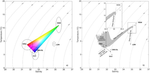
Table 1. Annually averaged temperature (˚C) and salinity used to describe the subsurface water from Cabot Strait (CBSS), the Cold Intermediate Layer formed in the GSL (CBS-CIL), Inshore Labrador Current (InLC) water, Warm Slope Water (WSW), and Labrador Slope Water (LSW). The averaged values over the 4-year 2011–2014 period used to study the variability at seasonal time scales are also included. The number inside parentheses represents one standard deviation.

	CBSS		CBS-CIL		InLC		WSW		LSW
	T	S	T	S	T	S	T	S	T	S
2011	3.92 (2.67)	31.67 (0.56)	2.37 (1.05)	32.53 (0.43)	0.35 (1.41)	32.60 (0.32)	8.15 (2.61)	35.03 (0.21)	3.98 (0.47)	34.86 (0.14)
2012	3.10 (2.32)	31.78 (0.45)	2.05 (0.79)	32.52 (0.44)	−0.62 (1.44)	32.78 (0.32)	12.46 (1.35)	35.51 (0.13)	4.20 (0.78)	34.82 (0.21)
2013	2.96 (2.97)	31.54 (0.83)	1.55 (1.07)	32.35 (0.53)	−0.27 (1.21)	32.62 (0.31)	13.38 (1.25)	35.71 (0.17)	3.86 (0.89)	34.79 (0.28)
2014	1.99 (3.47)	31.57 (0.49)	1.15 (1.40)	32.41 (0.52)	−0.83 (1.03)	32.75 (0.30)	12.80 (1.85)	35.58 (0.26)	4.09 (1.00)	34.86 (0.12)
Average	2.99 (2.86)	31.64 (0.58)	1.78 (1.08)	32.45 (0.48)	−0.35 (1.27)	32.69 (0.31)	11.70 (1.76)	35.46 (0.19)	4.02 (0.78)	34.83 (0.19)

For the seasonal variability of the hydrography, the temperature and salinity averaged over the 2011–2014 period are used for each endmember (Table 1). The use of annual endmembers has the advantage of capturing the interannual variability in the T-S characteristics of the relevant water masses, which can be very large. Indeed, Table 1 shows that the characteristics of each endmember can vary significantly interannually, with an especially warm event in 2012 (Hebert, Pettipas, Brickman, & Dever, 2013). Such an approach allows a more accurate estimation of the annual contribution of each water mass to the T-S distribution along the HL.

2 Glider data

From June 2011 to September 2014, 59 transects were completed along the HL using Teledyne Webb Research Slocum electric gliders (Fig. 3). The gliders are autonomous underwater vehicles that are able to sample the water column down to 200 m depth by changing their buoyancy using a ballast pump. Some of the induced vertical momentum of the glider is transferred to horizontal momentum by the wings installed on each side, resulting in a saw-tooth sampling pattern. The horizontal and vertical resolutions of the gliders’ datasets were, therefore, not uniform and depended on the angle of attack of the glider (about 22 to 26 degrees from the horizontal), the average speed of the glider (∼0.3 m s⁻¹), the depth of the water column, and the speed of the glider relative to the surrounding water. The glider data have an average vertical resolution of about 0.3 m and a finest horizontal resolution of approximately 850 m. Depending on the spatial coverage of the mission, it took from 3 to 11 days for the glider to complete a survey of the HL, during which pressure, temperature, conductivity, and other variables were recorded. Both salinity and potential density were computed using the Gibbs Seawater toolbox in MATLAB (McDougall & Barker, 2011). Observations made by the glider along each transect were gridded on a 0.5 m × 1 km grid in the vertical and horizontal directions, respectively. Because the glider sampled at 0.5 Hz (i.e., each transect includes between 150,000 and 450,000 data points), no interpolation was necessary to bin the glider data onto the spatial grid and a simple two-dimensional averaging block was used while still preserving the main hydrographic features. Seasonally averaged transects were produced for winter (January to March), spring (April to June), summer (July to September), and fall (October to December). Because the speed of the glider is relatively slow, it is important not to consider individual glider transects as either a snapshot or a time series of the conditions along the HL. Although this is not an issue in this study, caution must generally be used when considering physical processes occurring at a synoptic time scale from the glider data.

Fig. 3 (a) Temporal coverage of the datasets collected by the ADCPs and underwater gliders. (b) Spatial coverage of each glider mission along the Halifax Line. Readers may refer to Fig. 1 for the geographical locations of the T-stations.

3 Mixing triangle and two-dimensional colour bar

The temperature and salinity measured by gliders are used in this study to describe the T-S distribution of the water sampled along the HL. Two mixing lines and two major axes of variability are identified in the T-S diagram (Fig. 2):

• A major mixing line connecting the WSW endmember to CBSS water.

• A “deep mixing line” that runs from the major mixing line towards the LSW endmember and fits the warm-salty tip of the T-S distribution (see enlargement in inset of Fig. 2b).

• An axis of variability along the temperature axis mainly affecting surface water that varies on a seasonal time scale and is caused by surface heat fluxes (Umoh & Thompson, 1994).

• An axis of variability that reflects mixing between the CBSS water found in the subsurface layer and the CIL observed along the HL and drives the interannual variability observed in the slope of the major mixing line.

Because the contribution of LSW to the water composition at the HL is relatively small compared with other water masses, it is omitted from the water mass analysis. A mixing triangle is defined using the CBSS and WSW endmembers, the third vertex being defined as the temperature and salinity average between InLC and CBS-CIL, to reflect the uncertainty associated with the origin of water parcels with hydrographic characteristics located in that region of the T-S space. To visualize the spatial distribution of all the T-S points, a two-dimensional colour bar is defined by projecting Maxwell’s triangle onto the mixing triangle, therefore, associating one unique colour with each T-S pair located inside the mixing triangle (Fig. 2a; Judd, 1935). In order to assign a colour to points lying outside the mixing triangle, those points were projected either

• Vertically onto the CBSS–WSW edge of the triangle: This applies to data points located above the major mixing line and below 30 m depth. It is justified by the fact that the variability is mainly driven by the net surface heat fluxes and is, therefore, purely vertical in the T-S space (Umoh & Thompson, 1994).

• Perpendicularly onto the other two sides of the mixing triangle.

The percentage P of each water mass was estimated for each data point by solving for P in the following set of equations:(1) (2) (3)

b Velocity observations

1 Acoustic depth current profiler data

Velocity measurements were made using bottom-mounted, upward-looking ADCPs at three locations over the inner part of the HL (T-stations; see Fig. 1b). Currents were almost continuously measured from April 2008 to April 2014 at stations T1, T2, and T3, with some data gaps caused by either instrument failures or delays between recovery and redeployment of an instrument (Fig. 3a). Currents were sampled every 30 min with a vertical bin size of 4 m, from 10 m off the bottom to 10 m from the surface. To study the seasonal cycle of the circulation over the inner Scotian Shelf, the observed currents over the 2008–2014 period were averaged to form a one-year-long time series. The horizontal components of the observed currents were rotated from the eastward and northward directions into the alongshore and cross-shore directions. Because Nova Scotia’s shoreline is irregular and does not have a clear orientation, the alongshore component is defined in this study as the direction in which the variance in the observed velocity fluctuations is maximized. This is possible because of the relatively shallow water depth and the important role of topographic steering in driving the NSC. The following equation is used to determine the alongshore direction (Emery & Thomson, 2001):(4) where (u, v) are the zonal and meridional velocity components. The prime denotes the deviation from the mean, and the overline is used as a symbol for the time average. Analysis of the ADCP currents using Eq. (4) yields an average angle of 58° from true North. For comparison, the direction perpendicular to the traditional HL has an angle of 48°T and previous studies used an angle of 68°T (Schwing, 1989, 1992b).

2 Glider-based velocity

Two estimates of currents can be retrieved from the Slocum glider. One estimate is solely based on the flight characteristics of the glider. The other is based on the in situ temperature and conductivity measurements collected by the glider itself. The depth-averaged currents were obtained by comparing the glider’s dead-reckoning positioning system with the true location. The former is based on a model of the flight characteristics of the glider and the latter is determined by a global positioning system (GPS) at each of the glider’s surfacings, which occurs every 6 hours on average. A more complete description of the method is given in Appendix A (Todd, Rudnick, & Davis, 2009). The velocity vectors not only represent the average current experienced by the glider over the sampled water column but are also time-averaged from one surfacing to the next. To generate the depth-averaged currents observed by gliders, each current estimate was made based on the following steps:

1. A correction was applied for the surface drift experienced by the glider during the time spent at the sea surface (see Appendix A).

2. The current estimate was assigned to the mid-point of the dive and to the average time since the last surfacing.

3. A linear transformation was applied to the current estimate, using a calibration based on concurrent ADCP data collected at the T-stations (see Appendix A).

4. The zonal and meridional directions were rotated to the glider’s cross-path and along-path directions.

5. A linear interpolation was made along the glider path to match the horizontal sampling resolution of the glider.

The above processing steps are important in order to use this product as a “reference” current velocity when calculating the cross-path geostrophic velocity.

The cross-path geostrophic currents were estimated using the density field computed from the temperature and conductivity measurements collected by the glider, using the following methodology. First, the geostrophic shear across the glider’s track was estimated based on thermal wind dynamics (Gill, 1982). The velocity shear was then vertically integrated assuming zero velocity at the bottom to compute the cross-path geostrophic velocity. An offset was added to the geostrophic velocity in order for the depth-averaged geostrophic velocity to match the cross-path component of the depth-averaged current deduced from glider drift. Finally a transect of the geostrophic velocity was constructed for each leg of a glider mission.

3 Seasonal variability along the Halifax Line

a Hydrography and Water Masses

Although some features of the seasonal cycle at the HL were previously examined using the archived measurements (Loder, Hannah, Petrie, & Gonzalez, 2003; Smith, Petrie, & Mann, 1978) or numerical simulations (Han, Hannah, Loder, & Smith, 1997), hydrographic observations made by gliders provide the first high-resolution observational dataset resolving both the seasonal and interannual variability along the HL. Figure 4 demonstrates that a two-layer system develops in the vertical in the winter with colder and fresher water overlying a warmer but saltier deep layer. The potential density is smallest in the upper layer over the first 30 km from the shore. This water mass is associated with the coastally trapped NSC and has a colder and fresher T-S signature than ambient shelf water (Loder et al., 2003). It is separated from the offshore shelf water by a sharp density front located between 40 and 60 km from the shore at the surface and intersects the bottom around the 100 m isobath, located approximately 25 km offshore.

Fig. 4 Gridded fields of glider-based temperature (°C; left column), salinity (middle column), and potential density (kg m^–3; right column) in winter (first row), spring (second row), summer (third row); and fall (fourth row) at the Halifax Line, averaged over the period from June 2011 to September 2014. The 4°C isotherm is used to define the Cold Intermediate Layer (CIL) and is represented as a thick line in the temperature transects. Blue denotes either cold (left), fresh (middle), or low-density (right) water, while red represents either warm (left), more saline (middle), or denser (right) water.

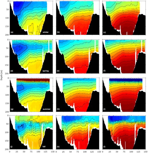
In spring, the vertical temperature structure shifts towards a 3-layer system as the surface water warms up and overlies the cold water located between 20 and 100 m, forming the so-called CIL (Fig. 4d; Loder et al., 2003; Umoh & Thompson, 1994). The CIL in spring provides a footprint of the ocean surface temperature experienced during the previous winter. The horizontal salinity gradient in the top layer decreases from winter to spring, as shown by the flattening of the isohalines above 100 m. Below 100 m, the temperature and salinity are very similar to those in the winter. The resulting density distribution shows a larger offshore horizontal density gradient close to the surface than in the winter but a more stable water column with only slightly tilted isopycnals. The low-density signature of the NSC is still identifiable inshore.

In summer, the surface temperature along the HL reaches a maximum and the water column is even more stratified. It is worth noting that the sea surface temperature over the shelf varies by more than 16°C over the course of a year while the core temperature of the CIL is not greatly affected by these seasonal changes. The 4°C isotherm traditionally defines the CIL over the Scotian Shelf and can be used to quantify the change in core temperature and spatial extent (Hebert et al., 2013). Averaged over the 2011–2014 period, the core temperature of the CIL (i.e., minimum temperature) warms up by 0.8°C (from 2.61° to 3.43°C) and the cross-sectional area shrinks from 2.48 to 0.68 km² from spring to summer.

Figure 4j demonstrates several interesting features in fall. The surface temperature becomes colder in fall than in the summer mainly because of the negative heat flux at the sea surface and increased wind-driven vertical mixing. A larger temperature drop occurs over the inner shelf, because of the increased advection of cold and fresh water coming from the GSL in fall. The CIL has experienced further erosion with a core temperature of 3.86°C and a cross-sectional area of 0.13 km². The temperature drop over the inner shelf is accompanied by the development of a coincident body of low-salinity water (S < 31), supporting the hypothesis that this water forms because of an increased inflow of low-salinity waters from the GSL. The inshore salinity reaches an annual minimum, creating the basis for the large horizontal density gradient observed in winter. The density field clearly shows the low-density signature of the water coming from the GSL over the inner Scotian Shelf. Nevertheless, isopycnals are still more horizontal than in winter, mainly because of the horizontal density front located at 50 m depth generated by the temperature distribution. It should be noted that large horizontal variations in the sub-surface (70–120 m) potential density at about 35 km from the coast in fall (Fig. 4l) are mainly caused by large horizontal variations in the sub-surface salinity (Fig. 4k). In 2012, the glider was caught in a flow reversal event, during which the current over the inner shelf was northeastward for a few days. Because of the fewer number of transects completed in fall, this 2012 singular event is reflected in the seasonal average.

The spatial distributions of the seasonal cycle in the hydrography at the HL are represented in Fig. 5, where the seasonal surface warming and cooling are clearly visible (grey dots). Using the water masses described in Section 2.a.1, and the colour scheme described in Section 2.a.3, a water mass analysis can be conducted using the high-resolution glider data. The analysis demonstrates that the water in the upper layer at the HL is mainly CBSS water and, therefore, originates from the GSL, with the highest percentage located over the inner shelf. For locations deeper or further offshore, the proportion of WSW increases, while the percentage of CBSS water decreases (Fig. 5). Indeed, the water located below the typical depth of Emerald Bank (i.e., 80 m) has T-S characteristics that resemble the WSW. The seasonal variability of the distribution of CBSS water along the HL follows the same pattern as the one for the low-density water previously described: in winter, CBSS water is more concentrated within the first 60 km from the shore and can penetrate as deep as 100 m. The distribution of CBSS water then shallows and spreads offshore with time to be mainly located in the upper 40 m of the water column and across the entire shelf along the HL in the summer months. The CBSS water still dominates the surface layer along the HL in the fall, although the percentage of WSW slowly increases, especially over the outer shelf (>70 km).

Fig. 5 Left panels present T-S diagrams based on glider observations at the Halifax Line for the 2011–2014 period winter (first row), spring (second row), summer (third row), and fall (fourth row). The colour scheme corresponds to Maxwell’s triangle (see Fig. 3). Endmembers are calculated for the 2011–2014 period and are represented as an ellipse centred on the centre of gravity of the observations in the corresponding region with the main axes representing the standard deviation of the temperature and salinity fields. Right panels show the distributions of corresponding transects using the same colour scheme in the four seasons. In all panels, the grey colour is associated with the observations collected within the top 30 m of the water column.

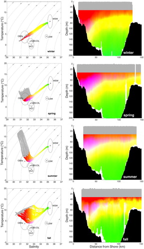
As mentioned in Section 2.a.1, the origin of the water found along the density front separating the CBSS water from the WSW (magenta in Fig. 5) is difficult to identify, because it lies in a region where the CBS-CIL and InLC ellipses overlap in the T-S space. It means that water from this region can either be composed of water coming from the CIL formed in the GSL, of InLC water, or more likely of a mix of both. Several pathways could explain the presence of InLC water along the HL: InLC water is known to penetrate the GSL through the Strait of Belle Isle as well as through the northeastern part of Cabot Strait (Galbraith et al., 2013). It is highly possible that the InLC water is then advected with the CBS-CIL out of the GSL and onto the Scotian Shelf. Another possible pathway would be a shelf intrusion through canyons and gullies located along the shelf break (Han & Loder, 2003).

b Alongshore Currents

Figure 6 shows that alongshore currents at the HL are largely dominated by the NSC, which is a strong southwestward coastal jet located in the upper 100 m and between 25 and 75 km offshore. Three ADCP mooring sites T1, T2, and T3 are located within the NSC’s pathway, with T1 and T3 located near the “edges” of the average flow and T2 located approximatively at the centre of the NSC. This is promising for the rest of this study because ADCP measurements were used to investigate the driving mechanisms of the NSC. The alongshore velocity exhibits a strong seasonal cycle that matches the one for the density field described in Section 3.a.

Fig. 6 Gridded fields of alongshore geostrophic currents (negative means southwestward) calculated from glider measurements of temperature, salinity, and depth-averaged currents in (a) winter, (b) spring, (c) summer, and (d) fall over the 2011–2014 period. The location of the T-stations are marked (dashed lines), and the extent of each section described in Section 5 is shown.

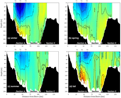
In winter, the tilting of isopycnal surfaces over the inner section of the HL is the steepest among the four seasons (Fig. 4c) and the southwestward component of the NSC is maximum and reaches about −0.2 m s⁻¹ (negative means southwestward) at T2 (Fig. 6a). Using the −0.05 m s⁻¹ isoline as the outer edge of the NSC, the NSC spreads over 60 km and reaches 100 m depth over the inner part of the HL in winter. A northeastward flow of about 0.1 m s⁻¹ also appears near the bottom between the 100 and 160 m isobaths (Fig. 6a). While a northeastward flow is also observed in the ADCP record, the intensity of this bottom flow seems large, which could be the result of the scaling of geostrophic currents using the estimated depth-averaged flow experienced by the glider (see Appendix A). A weak (<0.05 m s⁻¹) northeastward flow also occurs over the offshore flank of Emerald Basin in winter, which could be associated with cyclonic flow that follows the basin’s edges (Han & Loder, 2003).

In spring, the NSC slows to less than −0.15 m s⁻¹, with a core still located close to T2. The NSC in spring does not spread as far offshore as in the winter and only penetrates to about 80 m in the vertical. Both the northeastward flows previously noticed also exist in the spring although the bottom flow below the NSC in spring is weaker than in winter.

In summer, the alongshore flow at the HL is generally weaker, and the NSC is at its weakest (>−0.1 m s⁻¹) compared with other seasons. It should be noted that the NSC has a spatial coverage similar to that in spring, and the near-bottom northeastward flows occur over a smaller area with weaker velocities in both spring and summer.

In fall, the southwestward NSC becomes stronger but narrower as it reaches its minimum spatial coverage with a width of about 45 km compared with the flow in summer. The NSC extends down only to about 70 m in the fall, which is shallower than in summer. This coincides with the persistent summer stratification and the flatter isopycnal surfaces in the fall in comparison with the wintertime conditions, as described in Section 3.a. This also explains the discrepancy between the annual salinity minimum and maximum alongshore flow: while the low-salinity water coming from the GSL is observed in the fall, the water column is still relatively stratified, flattening the density front and, therefore, directly affecting the computed geostrophic velocity. Both northeastward flows reach their annual maximum along the 150 m isobath on both flanks of Emerald Basin. The sharp transition of alongshore geostrophic currents located about 35 km offshore in fall is associated with the large horizontal density gradients shown in Fig. 4l.

The seasonal cycle of the daily alongshore transport associated to the NSC (i.e., between T1 and T3, or section A) was calculated using the currents observed by the ADCPs at three T-stations over the 6-year 2008–2014 period (Fig. 8b). The 6-year averaged daily alongshore transport over section A of the HL is southwestward (i.e., negative), with a maximum amplitude in winter (∼−0.7 Sv, 1 Sv = 10⁶ m³ s^–1) and a minimum in summer (∼−0.2 Sv). The alongshore transport variability is larger in winter than in summer (Fig. 8a), which suggests that local winds should have a significant effect on the alongshore transport. The surface winds are usually stronger in winter than in summer on the Scotian Shelf. In addition to the large seasonal variability of the alongshore transport, there are also significant temporal variabilities at synoptic and interannual timescales (Fig. 8a).

4 Interannual variability along the Halifax Line and the 2012 warm anomaly

a Hydrography and Water Composition

The observation period of glider measurements includes a warm anomaly that was observed in 2012 over the Scotian Shelf and Gulf of Maine (Hebert et al., 2013). This strong anomalous event combined with the extensive temporal coverage of glider missions provides an opportunity to investigate the interannual hydrographic variability along the HL and the main physical processes involved. Other long-term monitoring programs such as AZMP have limited sampling frequencies, therefore, lack the temporal resolution necessary to avoid aliasing (Mann, 1969; Mann & Needler, 1967; Petrie, 2004).

In comparison with the surface temperature averaged over the 1981–2010 period, surface waters in 2012 were reported to be 1.0°C warmer at Halifax and between 2° and 2.5°C warmer over Emerald Basin. The temperature anomaly measured at 50 m depth in Emerald Basin is the same as in the surface water, but the anomaly at 250 m only reaches 0.7°C. Although the exact dynamics responsible for the warm anomalies that affect the entire water column along the HL are not well understood, plausible mechanisms include the following:

• A larger amount of shelf water at the HL came from a warm water mass (i.e., WSW) in 2012 than in other years.

• A smaller amount of the water along the HL came from a colder water mass (i.e., CBS-CIL or InLC) in 2012 than in other years.

• The relative contributions of the different water masses in 2012 were similar to other years, but the temperature signature of one, or several, contributing water masses is anomalously warm (i.e., the warm anomaly is advected into the domain).

Examining the seasonally averaged time series of the respective contributions of CBSS water, CBS-CIL or InLC, and WSW over the 2011–2014 period can shed light on the possible mechanisms responsible for the 2012 anomaly (Fig. 7). The analysis confirms the features described in Section 3.a: in the subsurface layer (30–50 m), CBSS water dominated and represented 81% of the water mixture on average, with a higher percentage over the inner shelf (Fig. 5). The WSW contribution was consistently low over this period, varying between 3 and 24% and averaging 13%. CIL water (InLC and CBS-CIL) also contributed to the water mixture in the subsurface layer, representing between 0 and 23% of the water composition. During 2012, an anomalously warm year, the respective contributions of the water masses considered did not exhibit a clear change. The percentage of CBSS water was higher than average (89–97%), and the contribution of CBS-CIL or InLC water was undetectable throughout all of 2012. Despite this relatively small change in water composition, this result suggests that the warming measured in the subsurface layer can be attributed to advection over the Scotian Shelf, rather than to a change in the relative contributions of the primary water masses. The annually defined endmembers demonstrate that, in 2012, the WSW was the only water mass that experienced a significant warming (i.e., larger than the observed standard deviation), with a positive change of 4.3°C compared with 2011 (Table 1). All other water masses had T-S characteristics similar to the other years in this study, within the observed standard deviation. It has also been suggested in the literature that part of the warming observed in the subsurface layer was a result of the combination of abnormally warm air temperature and an increase in surface heat influxes over the northeastern United States and Canadian regions (Chen, Gawarkiewicz, Kwon, & Zhang, 2015; Hebert et al., 2013).

Fig. 7 Time series of the seasonally averaged proportion (%) over the entire HL of the Cabot Strait subsurface water (CBSS, squares), Warm Slope Water (WSW, circles), and the average between Inshore Labrador Current water (InLC) and Cabot Strait Cold Intermediate Layer water (CBS-CIL, triangles) between 30 and 50 m (upper panel), 50 and 100 m (middle panel), and between 100 and 200 m (lower panel). The percentages are calculated using the method and equations described in Section 2.a.3.

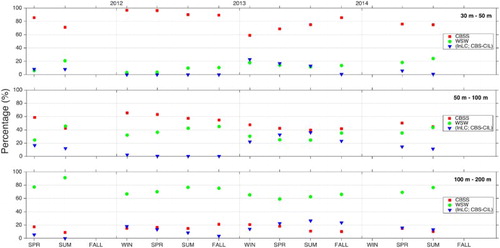
The layer lying between 50 and 100 m at the HL had similar characteristics: the contribution of CBSS water to the water mix was fairly constant (between 40 and 66%), and WSW contributed approximatively 35%, on average. As expected, the average contribution of InLC or CBS-CIL water is larger in this part of the water column (14%), with again a significant decrease occurring during 2012. Because the CBS-CIL and InLC are responsible for the presence of colder water in this layer, a decrease in their contributions to the water composition would consequently result in an increase in water temperature. Because WSW also contributed significantly to the water composition between 50 and 100 m, it appears that the warming observed in 2012 in this layer is due to the advection of anomalously warm WSW combined with a smaller percentage of cold water coming from the InLC and the CBS-CIL.

In the lower water column, between 100 and 200 m, the water mass composition was largely dominated by the WSW, with an average concentration of 71% over the 2011–2014 period. The CBSS water represented 15% of the water mass composition on average, while the cold water coming from the InLC or the CBS-CIL accounted for 15% of the water mixture. The interannual variability does not show any significant anomaly in the water mass distribution in 2012. The warm anomalies measured at depth can, therefore, be attributed to anomalously warm WSW being introduced onto the shelf, as opposed to a change in the water mass distribution.

b Alongshore Transport

Although the depth-integrated alongshore transport calculated from ADCP measurements between T1 and T3 had significant variability at synoptic time scales, the inferred alongshore transport exhibited a clear seasonal cycle each year (Fig. 8). Both the amplitude of the alongshore transport and the timing of the winter maximum were consistent over the 2008–2014 period, with an exception in 2012. The low-frequency anomaly of the alongshore transport shown in Fig. 8c exhibits a positive anomaly in 2012, with a maximum of about 0.25 Sv in the 2011–12 winter. This large positive transport anomaly was associated with the weakened NSC during this period. Some large anomalies also occurred in 2013: the winter maximum spreads out more in 2013 than in previous years, resulting in a negative anomaly of 0.35 Sv in the late winter. The alongshore transport was anomalously weak in the summer of 2013, generating a positive anomaly of about 0.1 Sv.

Fig. 8 (a) Daily-averaged alongshore transport and (b) average seasonal cycle in Sv (negative means southwestward) between T1 and T3 computed using ADCP measurements over the 2008–2014 period. A 50-day moving average was used to smooth the high-frequency variability of the time series. (c) Low and (d) high-frequency transport anomaly (Sv) calculated by subtracting the smoothed and raw curves in (b) from the ones in (a).

The high-frequency anomaly of the alongshore transport over section A of the HL is statistically similar from one year to the next and does not appear to be anomalous in 2012 (Fig. 8d). As suggested by previous studies (Schwing, 1992a, 1992b), local winds play a significant role in the temporal variability in the alongshore transport at synoptic time scales. By comparison with other years, the high-frequency transport anomaly does not present any peculiar features (Fig. 8d), which suggests that the anomalously weakened alongshore transport observed in 2012 was not likely a result of local surface winds.

5 Dynamics of the Nova Scotia Current

Previous studies suggested that the transport variability observed over the inner part of the HL is correlated with the outflow variability from the GSL through Cabot Strait (Drinkwater et al., 1979; Galbraith et al., 2014). Unfortunately, no observational datasets were collected over the 2008–2014 period to be used for the estimation of the transport across Cabot Strait. In this study, the monthly mean estimate of St. Lawrence River runoff at Québec provided by the Maurice Lamontagne Institute was used to assess the influence of the St. Lawrence River on the circulation over the Scotian Shelf (Bourgault & Koutitonsky, 1999; Galbraith et al., 2014). The focus here is on the peak-to-peak correlation between the two time series to quantify how long the seasonal pulse in the St. Lawrence River discharge takes to reach the HL and the level of correlation between the two transport estimates. The cross-covariance function between the St. Lawrence River discharge and the negative value of the alongshore transport between T1 and T3 reveals that these two time series have significant covariance at a 9-month lag (Fig. 9). The normalized covariance is relatively large considering that both systems are more than 1500 km apart. This is consistent with the estimation of a 3-month lag found by Drinkwater et al. (1979) between Cabot Strait and the HL, as the distance between Halifax and Québec is approximatively three times as large as the one between the HL and Cabot Strait.

Fig. 9 Left panel presents the normalized cross-covariance function between the monthly mean estimate of the St. Lawrence River runoff at Québec (Bourgault & Koutitonsky, 1999; Galbraith et al., 2014) and the negative transport computed from the ADCP records at three stations. The 95% confidence intervals (dashed lines) calculated using , where N is the number of observations, are superimposed. The two time series are shown in the right panel for the 2008–2014 period.

Based on the relationship between the freshwater outflow from the St. Lawrence River and the NSC, it can be argued that baroclinicity plays an important role in the dynamics of the coastal currents in the GSL and Scotian Shelf. The alongshore baroclinic transport (Gill, 1982) was, therefore, computed for all the glider transects collected since 2011 over four sections (Fig. 10e). Section A covers the distance between T1 and T3; section B corresponds to Emerald Basin; section C is located over Emerald Bank; and section D extends from Emerald Bank to the shelf break. Figure 10a presents a comparison of the geostrophic transport computed from the glider’s transects and the daily transport based on ADCP measurements. The two time series are significantly correlated (r = 0.80, p < 0.05), which demonstrates that geostrophy can be used to quantify the low-frequency transport across the HL as the first order of accuracy. Any discrepancy between the geostrophic transport estimated using glider data and the alongshore transport based on the ADCP measurements could be attributed to the barotropic component of the flow, such as the wind-driven currents which were ignored when estimating geostrophic currents. In this case, the thought process is not straightforward because geostrophic velocities are scaled using the glider drift, which indirectly includes part of the barotropic flow (see Appendix A).

Fig. 10 Time series of geostrophic transport (negative means southwestward) over four different sections of the Halifax Line ((a) through (d)) computed from glider transects (filled squares). The daily averaged transport estimated from ADCP measurements between T1 and T3 is shown (dashed line) in (a) and the extent of each section is shown in (e)

The alongshore transport at the HL is larger through section A of the HL than over any of the other sections (Fig. 10), which is consistent with the fact that the core of the NSC occupies section A. The two time series of alongshore transports depicted in Fig. 10a exhibit the same seasonal cycle described above: an intense alongshore transport in winter and a weakened transport in summer through section A during the study period between June 2011 and September 2014. The alongshore transport through section B was occasionally large during this period, particularly for the first half of 2012 (Fig. 10b). This can be explained by the episodic offshore displacement of the NSC, often due to upwelling-favourable wind events. Even though fewer data points are available for sections C and D, the alongshore transport through these two sections was significantly smaller and can be either negative (southwestward) or positive (northeastward) during the study period (Figs 10c and 10d).

To further examine the temporal and spatial variability of the NSC, an Empirical Orthogonal Function (EOF) analysis was conducted using the daily-averaged alongshore currents measured by ADCPs at T1, T2, and T3 during the 2008–2014 period. The first two EOF modes (EOF1 and EOF2) contain approximately 95% of the variance (Fig. 11). The first mode (EOF1) explains between 78 and 92% of the observed variability of the alongshore currents during the study period. The vertical structure of EOF1 is similar at the three stations, which features a surface intensified flow and monotonically decreasing currents below the sea surface. The main difference at the three stations lies in the time series of the mode coefficient. Although it does not seem to follow any sort of seasonal pattern at T1, the mode coefficients of the first mode at T2 and T3 have a pronounced seasonal cycle. It should be noted that the EOFs were computed using the current anomalies from the annual mean, which means that a positive mode coefficient at T2 and T3 does not necessarily imply a northeastward flow but only a positive anomaly with respect to the annual-mean flow. The colour plots in Fig. 11 represent the reconstructed alongshore currents using EOF1 (third row) and EOF2 (sixth row), with the inclusion of the annual mean alongshore currents. Because the first EOF explains more than 77% of the observed variability at the three stations, the reconstructed flow based on EOF1 and the annual mean flow can be used to approximate the ADCP observations as the first order of accuracy. Figure 11a demonstrates that at T1 the reconstructed flow based on EOF1 is highly variable in time, although consistently southwestward. Two flow reversal events occurred in February and April, when the flow associated with EOF1 turned northeastward (positive). At stations T2 and T3, the reconstructed flow using EOF1 has a large seasonal cycle. At these two stations, the reconstructed surface currents are strong in winter and weakened in summer, with a stronger flow at T2 than at T3, in agreement with the current maximum being located at T2. The seasonal cycle in the thickness of the NSC is also well reconstructed and agrees reasonably well with the pattern of the geostrophic flow shown in Fig. 6. By using the −0.05 m s⁻¹ isoline as the edge of the NSC, the current reaches a depth of about 130 m at T2 and about 110 m at T3 in the winter and shoals to about 70 m in the summer at T2.

Fig. 11 Mode coefficients and patterns of the first (top three rows) and second (bottom three rows) EOFs calculated from the daily-averaged annual time series of observed alongshore currents at T1, T2, and T3 over the 2008–2014 period (negative means southwestward). For each mode, the vertical profile of the EOF, the mode coefficient, and the corresponding reconstructed flow are shown. The annual mean flow was included in the flow reconstruction based on the EOF. The percentage of variability explained by each mode is also indicated.

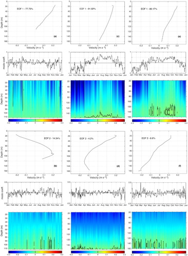
All the above-mentioned features in the reconstructed flow based on EOF1 (as well as the annual-mean currents) suggest that the first mode is tied to the alongshore baroclinic flow and, therefore, describes the buoyancy-driven flow generated by the density gradient between coastally trapped GSL water being advected southwestward and ambient shelf water. The high percentage of variability of alongshore current explained by this forcing mechanism highlights the strong connectivity between the GSL and the circulation over the Scotian Shelf.

The second EOF (EOF2) explains about 14, 4, and 6% of the observed variability of the alongshore currents measured by ADCPs at T1, T2, and T3, respectively. The vertical structure of EOF2 is characterized by a vertical profile that decreases rapidly with depth and changes sign at about 50 m depth (Figs 11b, 11d, and 11f). The mode coefficients of EOF2 are small (≤0.3) in comparison with EOF1. The time series of mode coefficients for EOF2 at the three stations do not have a clear seasonal cycle although the variability of EOF2 is relatively higher in winter than in summer. The reconstructed currents at three stations based on EOF2 have a maximum current less than ±0.06 m s⁻¹ in amplitude, which is less than half the strength of the currents explained by EOF1. The reconstructed flow based on EOF2 at stations T1 and T3 is relatively large in the top 30 m and near zero below 30 m. In comparison, the reconstructed flow based on EOF2 at station T2 can reach depths greater than 70 m. The second mode of variability is arguably linked to local wind forcing for the following reasons. First, the percentage of current variability explained by EOF2 is much larger at T1 than at T2 or T3. This concurs with previous observations that surface wind stress has a greater impact on the flow close to shore and, therefore, explains more of the current variability (Schwing, 1989). Second, the time series of the mode coefficient for EOF2 shows the expected seasonal cycle for local winds, with higher values and variability in fall and winter than in spring and summer. This corresponds to the observed seasonal cycle of the alongshore wind over the Scotian Shelf (Petrie, Topliss, & Wright, 1987): stronger winds than average in winter and weaker winds during summer.

The lack of a significant correlation between the mode coefficients for EOF2 and the wind speeds measured outside Halifax Harbour (not shown) suggests, however, that other mechanisms might also be involved in the variability of this mode. Indeed, if local winds were to entirely force this mode, the mode coefficients at T1, T2, and T3 would be expected to be highly coherent because the wind forcing would not vary significantly over the distance of about 35 km separating the three T-stations.

6 Summary and conclusions

High-quality and concurrent datasets of currents and hydrography were collected at high temporal and spatial resolutions along the HL, which provides a unique opportunity to better understand the seasonal and interannual variability of circulation and hydrography over the Scotian Shelf. Analysis of glider-based repeated surveys of temperature and salinity along the HL demonstrated that only the top 100 m of the water column at the HL was strongly affected by the seasonal cycle during the 6-year study period of 2008–2014. Although salinity at the HL did not vary significantly throughout the year during the study period, the observed temperature in the top few metres at the HL had large temporal variations of more than 16°C from winter to summer, mainly due to local processes associated with the net heat flux at the sea surface (Umoh & Thompson, 1994). As the slope of the superimposed isopycnals in Fig. 5 suggests, the density distribution at the HL was mainly determined by the salinity field, but temperature plays an important role in the upper water column stratification, particularly in the summer and fall when the surface water is warmer.

The analysis of hydrographic observations during the study period demonstrated that the T-S distribution in the subsurface layer (30 to 50 m) at the HL was affected by water originating from the GSL (CBSS water), which contributes approximatively 81% of the water composition, while the WSW was responsible for 13%, on average. The colder water observed in this layer cannot be distinguished between water coming from the CBS-CIL or the InLC because they have similar signatures in the T-S space. Nevertheless, this water mass contributed about 6% of the water mixture in this layer. Water from the GSL (i.e., CBSS water) was primarily contained inshore (<60 km) and created the density gradient associated with the NSC. Over deep water areas and further offshore, the contribution of water coming from the Scotian Shelf break increased. The influence of the colder water coming from either the CBS-CIL or the InLC was mainly observed at mid-depth, representing 14% of the water composition between 50 and 100 m. The WSW dominated the water mixture below 100 m, representing 71% of the water composition.

Annually averaged endmembers of water masses influencing the hydrographic conditions over the Scotian Shelf were important to resolve the respective contributions of the different water masses at the HL during the study period. The interannual variability in the salinity field was relatively small in comparison with the observed temperature field. Indeed, the WSW experienced a large warming in 2012, with an increase of more than 4°C. Although the InLC and CBS-CIL had overlapping endmember ellipses and could not, therefore, be distinguished as two separate water sources along the HL, the interannual variability in the contributions of the different water masses suggested that the 2012 warm anomaly was mostly a result of the advection of anomalously warm water from the offshore region. This warm event was reinforced by the smaller inflow of cold water coming from the CBS-CIL and the InLC.

The NSC flowed southwestward along the south coast of Nova Scotia, and its transport had a seasonal cycle associated with the St. Lawrence River discharge with a 9-month lag at the HL, further highlighting the important contribution of the GSL to oceanic conditions over the Scotian Shelf. This coastally trapped current was surface intensified, centred approximately 40 km offshore (i.e., T2). The NSC had a maximum transport of about 0.8 Sv in the winter during the study period. Almost all the observed temporal variability of the alongshore flow measured within the NSC can be explained by the first two EOFs. The first EOF itself explains between 78 and 92% of the current variability, depending on the mooring location on the HL. Based on the vertical profile and the strong seasonal cycle in the mode coefficient of the first mode, the variability can be related to the baroclinic alongshore transport associated with the buoyant water coming from the GSL. The second mode of variability explains between 4 and 14% of the NSC variability and seems to be associated with local wind forcing.

By combining both hydrographic and current velocity observations collected at high temporal and spatial resolutions over several years, this study provides a characterization of the conditions over the Scotian Shelf. The simultaneous descriptions of both the seasonal cycle and interannual variability in temperature, salinity, and alongshore currents become possible, as opposed to previous studies based on climatologies or sparse and infrequent observations.

Appendix A. Glider-based geostrophic velocity

An algorithm was used to estimate the vertically integrated current experienced by a glider once it reached the sea surface. The algorithm is described below and depicted in Fig. A1.

Fig. A1 Schematic showing the algorithm used to estimate depth-averaged currents from the glider drift. Ta refers to the time when the glider dives; Tb and Tb′ correspond to the surfacing times; Tc is the time stamp for the first GPS fix; Td refers to the time stamp of the second GPS fix; and T_middle is the middle point of the glider’s dive. The solid line represents the path of the glider as extrapolated by dead reckoning. The red arrow represents the depth-averaged current experienced by the glider between the last two surfacings; the blue arrow represents the depth-averaged current calculated by the glider and the green arrow represents the surface drift.

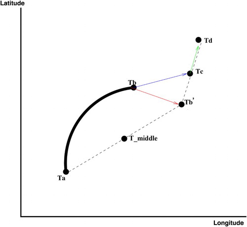
We consider that the glider acquires a GPS fix at time Ta, dives and then surfaces at time Tb. The thick line between Ta and Tb in Fig. A1 represents the extrapolated path using a dead reckoning algorithm. The glider “thinks” it surfaces at Tb but actually surfaces at Tb′, because of the current it experienced during the dive. The red arrow is then the depth-averaged current that affected the glider trajectory over the Ta-to-Tb time period.

The main issue is that the first GPS fix does not occur at Tb′ (i.e., exactly when the glider surfaces) but at a later time Tc. The deduced current is, therefore, the blue arrow in Fig. A1, which also includes the surface drift occurring between the time of surfacing (Tb′) and the first GPS fix (Tc).

To correct for this surface drift, the glider obtains a second GPS fix at a later time Td. It can, therefore, calculate the surface drift by dividing the difference in positioning at times Tc and Td by the time elapsed between Tc and Td (green arrow). The location of the glider at time Tb′ can be extrapolated by using this estimation of the surface drift and subtracting it from the glider’s position at time Tc. This technique provides a more accurate estimate of the depth-averaged current experienced by the glider during its last dive.

Each of these depth-averaged current estimations are then associated with the coordinates of the middle point of the glider’s dive (T_middle). All surfacings located within a 2 km radius from an ADCP mooring (T1, T2, or T3; Fig. 1b) are used to compare gliders’ current estimates to depth-averaged ADCP measurements. A linear fit is calculated and applied to all glider-based current estimate to calibrate the dataset with the ADCP observations ( Fig. A2).

Fig. A2 Comparison between the depth-averaged, cross-shore (U, left) and alongshore (V, right) currents measured by one of the ADCPs located at the T-station and the depth-averaged current experienced by the glider during a dive within a 2 km radius from an ADCP station. The goodness of fit R² between glider-based and ADCP observations is indicated for the non-calibrated datasets (1:1 line, solid line), as well as for the calibrated glider-based current using the linear equation indicated in the figures (best fit, dashed line).

Geostrophic currents are calculated using the thermal wind equation (Gill, 1982), based on the potential density indirectly measured by the glider. The data is gridded at a resolution of 1 km in the horizontal direction and 0.5 m in the vertical. The horizontal gradient in density is calculated using 2nd order finite differencing over 16 km, which corresponds to the internal Rossby radius of deformation in this region (Gill, 1982).

The velocity shear is then vertically integrated assuming a zero-velocity at the bottom. An offset is added to the geostrophic velocity so that the depth-averaged geostrophic velocity matches the across-path depth-averaged current deduced from glider drift. Plots of geostrophic currents superimposed with observations have been produced and demonstrate that this method yields very good comparisons (not shown).

Acknowledgements

We wish to thank Roger Pettipas, Richard Davis, Adam Comeau, and Jon Pye for making the required datasets available. We would also like to thank Brian Petrie for useful discussions and comments.

Disclosure statement

No potential conflict of interest was reported by the authors.

Additional information

Funding

This research was supported by the Ocean Tracking Network (OTN), through a network project grant NETGP [grant number #375118-08] from the Natural Sciences and Engineering Research Council of Canada (NSERC) with additional support from the Canadian Foundation for Innovation (CFI) [grant number #13011], and the Social Sciences and Humanities Research Council (SSHRC) [grant number #871–2009-0001].

References

- Anderson, C., & Smith, P. (1989). Oceanographic observations on the Scotian Shelf during CASP. Atmosphere-Ocean, 27, 130–156. doi: 10.1080/07055900.1989.9649331
- Bourgault, D., & Koutitonsky, V. G. (1999). Real-time monitoring of the freshwater discharge at the head of the St. Lawrence Estuary. Atmosphere-Ocean, 37(2), 203–220. doi: 10.1080/07055900.1999.9649626
- Chen, K., Gawarkiewicz, G., Kwon, Y.-O., & Zhang, W. G. (2015). The role of atmospheric forcing versus ocean advection during the extreme warming of the northeast U.S. continental shelf in 2012. Journal of Geophysical Research: Oceans, 120, 4324–4339. doi:10.1002/2014JCO10547.
- Drinkwater, K., Petrie, B., & Sutcliffe, W. (1979). Seasonal geostrophic volume transports along the Scotian Shelf. Estuarine and Coastal Marine Science, 120(6), 4324–4339.
- Emery, W. J., & Thomson, R. (2001). Data analysis methods in physical oceanography. Amsterdam, New York: Elsevier.
- Galbraith, P. S., Chassé, J., Gilbert, D., Larouche, P., Caverhill, C., Lefaivre, D., … Lafleur, C. (2014). Physical oceanographic conditions in the Gulf of St. Lawrence in 2013. DFO Canadian Science Advisory Secretariat, Document, 2014/062. Ottawa, Ontario.
- Galbraith, P. S., Chassé, J., Larouche, P., Gilbert, D., Brickman, D., Pettigrew, B., … Lafleur, C. (2013). Physical oceanographic conditions in the Gulf of St. Lawrence in 2012. DFO Canadian Science Advisory Secretariat, Document, 2013/026. Ottawa, Ontario.
- Gatien, M. G. (1976). A study in the slope water region south of Halifax. Journal of the Fisheries Research Board of Canada, 33(10), 2213–2217. doi: 10.1139/f76-270
- Gilbert, D., & Pettigrew, B. (1997). International variability (1948–1994) of the CIL core temperature in the Gulf of St. Lawrence. Canadian Journal of Fisheries and Aquatic Sciences, 54(S1), 57–67.
- Gill, A. E. (1982). Atmosphere-ocean dynamics (Vol. 30). London, UK: Academic Press.
- Han, G., Hannah, C., Loder, J., & Smith, P. (1997). Seasonal variation of the three-dimensional mean circulation over the Scotian Shelf. Journal of Geophysical Research, 102(C1), 1011–1025. doi: 10.1029/96JC03285
- Han, G., & Loder, J. W. (2003). Three-dimensional seasonal-mean circulation and hydrography on the eastern Scotian Shelf. Journal of Geophysical Research: Oceans, 108(C5), 1–21. doi: 10.1029/2002JC001463
- Hebert, D., Pettipas, R., Brickman, D., & Dever, M. (2013). Meteorological, sea ice and physical oceanographic conditions on the Scotian Shelf and in the Gulf of Maine during 2012. DFO Canadian Science Advisory Secretariat, Document, 2013/058. Ottawa, Ontario.
- Judd, D. B. (1935). A Maxwell triangle yielding uniform chromaticity scales. Journal of the Optical Society of America, 25(1), 24–35. doi: 10.1364/JOSA.25.000024
- Khatiwala, S. P., Fairbanks, R. G., & Houghton, R. W. (1999). Freshwater sources to the coastal ocean off northeastern North America: Evidence from H2 18O/H2 16O. Journal of Geophysical Research, 104(C8), 18241–18255. doi: 10.1029/1999JC900155
- Loder, J., Han, G., Hannah, C., Greenberg, D., & Smith, P. (1997). Hydrography and baroclinic circulation in the Scotian Shelf region: Winter versus summer. Canadian Journal of Fisheries and Aquatic Sciences, 54(S1), 40–56. doi: 10.1139/f96-153
- Loder, J., Hannah, C., Petrie, B., & Gonzalez, E. (2003). Hydrographic and transport variability on the Halifax Section. Journal of Geophysical Research, 108(C11), 1–18. doi: 10.1029/2001JC001267
- Mann, C. (1969). A summary of variability observed with monitoring sections off the east and west coasts of Canada. Progress in Oceanography, 5, 17–30. doi: 10.1016/0079-6611(69)90024-X
- Mann, C., & Needler, G. (1967). Effect of aliasing on studies of long-term oceanic variability off Canada’s coasts. Journal of the Fisheries Research Board of Canada, 24(8), 1827–1831. doi: 10.1139/f67-150
- McDougall, T., & Barker, P. (2011). Getting started with TEOS-10 and the Gibbs Seawater (GSW) Oceanographic Toolbox. SCOR/IAPSO WG127. ISBN 978-0-646-55621-5.
- McLellan, H. J. (1954). Temperature-salinity relations and mixing on the Scotian Shelf. Journal of the Fisheries Research Board of Canada, 11(4), 419–430. doi: 10.1139/f54-028
- Petrie, B. (2004). The Halifax Section: A brief history. Atlantic Zone Monitoring Program Bulletin, 4, 26–29. Retrieved from http://www.meds-sdmm.dfo-mpo.gc.ca/isdm-gdsi/azmp-pmza/publications-eng.html.
- Petrie, B. (2007). Does the North Atlantic Oscillation affect hydrographic properties on the Canadian Atlantic continental shelf? Atmosphere-Ocean, 45(3), 141–151. doi: 10.3137/ao.450302
- Petrie, B., & Drinkwater, K. (1993). Temperature and salinity variability on the Scotian Shelf and in the Gulf of Maine 1945–1990. Journal of Geophysical Research: Oceans, 98(C11), 20079–20089. doi: 10.1029/93JC02191
- Petrie, B., Topliss, B., & Wright, D. (1987). Coastal upwelling and eddy development off Nova Scotia. Journal of Geophysical Research, 92(C12), 12979–12991. doi: 10.1029/JC092iC12p12979
- Schwing, F. B. (1989). Subtidal response of the Scotian Shelf bottom pressure field to meteorological forcing. Atmosphere-Ocean, 27(1), 157–180. doi: 10.1080/07055900.1989.9649332
- Schwing, F. B. (1992a). Subtidal response of Scotian Shelf circulation to local and remote forcing. Part II: Barotropic model. Journal of Physical Oceanography, 22(5), 542–563. doi: 10.1175/1520-0485(1992)022<0542:SROSSC>2.0.CO;2
- Schwing, F. B. (1992b). Subtidal response of Scotian Shelf circulation to local and remote forcing. Part I: Observations. Journal of Physical Oceanography, 22(5), 523–541. doi: 10.1175/1520-0485(1992)022<0523:SROSSC>2.0.CO;2
- Smith, P., Petrie, B., & Mann, C. (1978). Circulation, variability, and dynamics of the Scotian Shelf and slope. Journal of the Fisheries Research Board of Canada, 35, 1067–1083. doi: 10.1139/f78-170
- Smith, P., & Schwing, F. (1991). Mean circulation and variability on the eastern Canadian continental shelf. Continental Shelf Research, 11, 977–1012. doi: 10.1016/0278-4343(91)90088-N
- Therriault, J.-C., Petrie, B., Pepin, P., Gagnon, J., Gregory, D., Helbig, J., … Sameoto, D. (1998). Proposal for a northwest Atlantic Zonal Monitoring Program. In Canadian technical report of hydrography and ocean sciences, 194. Ottawa, Ontario: DFO.
- Thompson, K. R., & Sheng, J. (1997). Subtidal circulation on the Scotian Shelf: Assessing the hindcast skill of a linear, barotropic model. Journal of Geophysical Research: Oceans (1978–2012), 102(C11), 24987–25003. doi: 10.1029/97JC00368
- Todd, R. E., Rudnick, D. L., & Davis, R. E. (2009). Monitoring the greater San Pedro Bay region using autonomous underwater gliders during fall of 2006. Journal of Geophysical Research: Oceans (1978–2012), 114(C6), 2156–2202. doi: 10.1029/2008JC005086
- Umoh, J. U., & Thompson, K. R. (1994). Surface heat flux, horizontal advection, and the seasonal evolution of water temperature on the Scotian Shelf. Journal of Geophysical Research: Oceans, 99(C10), 20403–20416. doi: 10.1029/94JC01620