The SST–Wind Coupling Pattern in the East China Sea Based on a Regional Coupled Ocean–Atmosphere Model

ABSTRACT

To study the interaction between sea surface temperature (SST) and surface wind in the East China Sea (ECS), the Coupled Ocean–Atmosphere–Wave–Sediment Transport (COAWST) modelling system is used to downscale a global atmospheric reanalysis product over the study area in 2013. A singular value decomposition (SVD) method is applied to SST and surface wind speed to study their coupling relationship in the ECS. The heterogeneous correlation map indicates that the surface wind has a negative correlation with the SST, especially in the Kuroshio Current. From lead-lag correlations between the first principal component of SST and surface wind SVD (filtered using a Lanczos high-pass filter with a 90-day cut-off), a correlation of about 0.1 is found at lag −6, and a negative correlation of about −0.3 is also found around lag 1. The results indicate a negative feedback between SST and wind fluctuations at short time-scales. Air–sea heat fluxes contribute little to the SST variability in the ECS section of the Kuroshio and the analysis of the mixed-layer heat budget shows that the contribution of horizontal advection is dominant in determining the intraseasonal SST signals.

RÉSumé

[Traduit par la rédaction] Nous étudions l’interaction entre la température de surface de la mer (SST) et le vent en surface dans la mer de Chine orientale en 2013, et ce, en réduisant l’échelle de réanalyses atmosphériques mondiales couvrant la région à l’étude, à l’aide du modèle Coupled Ocean-Atmosphere-Wave-Sediment Transport (COAWST). Nous appliquons une décomposition en valeurs singulières (DVS) à la SST et à la vitesse du vent en surface, afin d’étudier leur lien dans la mer de Chine orientale. La carte de corrélation hétérogène indique que le vent en surface possède une corrélation négative avec la SST, particulièrement dans le Kuroshio. À partir de corrélations décalées entre la première composante principale issue de la DVS pour la SST et le vent en surface (filtrée à l’aide d’un algorithme de Lanczos passe-haut avec coupure à 90 jours), nous avons trouvé une corrélation d’environ 0,1 pour un décalage de −6 et une corrélation négative d’environ −0,3 près du décalage de 1. Les résultats indiquent une rétroaction négative entre les fluctuations de la SST et du vent pour de courtes échelles temporelles. Les flux de chaleur air-mer contribuent peu à la variabilité de la SST dans la portion du Kuroshio se trouvant dans la mer de Chine orientale. L’analyse du bilan de chaleur de la couche de mélange montre que la contribution de l’advection horizontale domine en ce qui concerne la détermination des signaux intrasaisonniers de la SST.

KEYWORDS:

• SST–wind coupling
• singular value decomposition
• East China Sea
• regional coupled ocean–atmosphere model

1 Introduction

Air–sea interaction is of great interest to atmospheric scientists and oceanographers. From past research, a negative correlation between sea surface temperature (SST) and surface wind was found at both synoptic and global scales (Wallace, Smith, & Jiang, 1990), which suggests that the ocean is forced by the atmosphere. The atmosphere drives the ocean through buoyancy change and wind, and the ocean affects the atmosphere through heat and moisture fluxes (Xie, 2004). The presence of oceanic fronts and eddies seems to counter those results at the oceanic mesoscale. For example, observations (Byrne, Papritz, Frenger, Munnich, & Gruber, 2015; Chelton et al., 2001, 2004; Frenger, Gruber, Knutti, & Münnich, 2013; Gaube, Chelton, Samelson, Schlax, & O’Neill, 2015; Ma, Xu, Dong, Lin, & Liu, 2015, 2016; Nonaka & Xie, 2003; O’Neill, Chelton, & Esbensen, 2003, 2005; Tokinaga, Tanimoto, & Xie, 2005, 2006; Vecchi, Xie, & Fischer, 2004; Xie, 2004; Xu & Xu, 2015, 2017; Xu, Tokinaga, & Xie, 2010) have shown that surface wind speed is higher over warm water and lower over cool water (i.e., a positive correlation that is opposite to that found on larger scales). The sensible heat flux (e.g., Vecchi et al., 2004) and the latent heat flux into the ocean have a negative correlation with mesoscale SSTs in various parts of the world ocean (e.g., Bryan et al., 2010; Haack, Chelton, Pullen, Doyle, & Schlax, 2008; Liu, Xie, & Niiler, 2007; Seo, Jochum, Murtugudde, Miller, & Roads, 2007, 2008). Oceanic mesoscale eddies contribute important horizontal heat and salt transports on a global scale (Dong, McWilliams, Liu, & Chen, 2014). It is important to understand the characteristics and mechanisms controlling these regional mesoscale anomalies in order to gain further insight into coupling processes controlling large-scale climate variation.

Perturbations of surface wind induced by SSTs can feed back to the ocean through both upper-ocean wind mixing and wind-driven upwelling, both of which can change SST, resulting in two-way coupling between the ocean and atmosphere on the synoptic scale. The feedback effects from SST-induced wind stress curl anomalies can significantly alter ocean circulations because Ekman pumping acts as a source of vorticity controlling the large-scale circulation of the ocean. Because wind stress curl anomalies associated with mesoscale SST variations are linearly related to the crosswind SST gradient (Chelton et al., 2001), the feedback effects of Ekman upwelling tend to be stronger where the SST gradient is oriented perpendicular to the wind.

Air–sea interactions can be examined by means of numerical models, which can provide fully coupled atmospheric-oceanic variables. Although there are many numerical studies based on global models (e.g., Deng & Xu, 2016; Pegion & Kirtman, 2008; Shukla & Zhu, 2014; Wu & Kirtman, 2005; Wu, Kirtman, & Pegion, 2006) and a few coupled models for the South China Sea (Fang, Zhang, Tang, & Ren, 2010; Li & Zhou, 2010; Ren & Qian, 2005), studies using high-resolution regional coupled models in the East China Sea (ECS) are limited, which is probably because of the highly complex topography and bathymetry of the region that require very high-resolution model grids to resolve continental shelves and/or slopes, straits, and archipelagos. Based on satellite observations and an idealized ocean–atmosphere coupled model, Chen, Liu, Tang, and Wang (2003) hypothesized that a significant air–sea interaction exists at the shelf-break front in the ECS. They found that the air–sea interaction, when combined with sloping topography, could provide a mechanism for the genesis of the shelf-break front. The resulting frontal circulation and vertical mixing could bring nutrient-rich subsurface water to the surface euphotic zone, thus making the frontal region an obvious place for primary production. Iwasaki, Isobe, and Kako (2014) developed a regional coupled atmosphere–ocean model based on the Pennsylvania State University–National Center for Atmospheric Research Mesoscale Model in conjunction with the Princeton Ocean Model to investigate coupled atmosphere–ocean processes that might occur over the Yellow Sea and ECS shelves in winter. In addition, one of the strongest western boundary currents, the Kuroshio Current, flows in this region. It is well known that western ocean boundary currents induce strong air–sea interactions. The complex structure of SST in the ECS can affect many important atmospheric phenomena on various time-scales. Xie et al. (2002) showed that a sharp SST front near the Kuroshio had a significant impact on the development of mesoscale low-pressure systems in the ECS during winter. Miyama, Nonaka, Nakamura, and Kuwano-Yoshida (2012) reported that high SSTs in the Kuroshio helped organize and maintain a well-defined convective rain band in May. Xu, Xu, Xie, and Wang (2011) showed that a spring Kuroshio front in the ECS influenced both boundary layer convergence and deep cumulus convection.

In this study, we used a regional coupled ocean–atmosphere model to downscale a global atmospheric reanalysis product over the ECS in 2013. We first validated the fully coupled model by comparing the SST and wind speed fields with those of satellite observations. We then performed singular value decomposition (SVD) on SST and 10 m wind speed in order to study the coupling between the two variables. The rest of the paper is organized as follows: the data used in this study and a description of the model configuration are presented in Section 2. The coupled model results of SST and wind speed fields are compared with satellite observations in Section 3. We also used a self-organizing map (SOM) to obtain four basic coherent SST and surface wind patterns. To investigate the interaction between the SST and surface wind, we performed SVD on the SST and 10 m wind speed. A summary is provided in Section 4.

2 Model

a Model description

We used the Coupled Ocean–Atmosphere–Wave–Sediment Transport (COAWST) modelling system (Warner, Armstrong, He, & Zambon, 2010), which includes three state-of-the-art numerical model components representing the atmosphere, ocean, and wave environments. We used the Weather Research and Forecasting (WRF), version 3.6.1, atmospheric model with the Advanced Research WRF (ARW) dynamical core (Skamarock et al., 2008). The WRF model is a next generation, fully compressible, non-hydrostatic, prognostic model suitable for idealized and realistic numerical simulations of the atmosphere, allowing for runs at different scales ranging from synoptic to mesoscale. The model uses a terrain-following hydrostatic-pressure coordinate in the vertical. The configuration used in this study has 40 vertical levels that are unevenly distributed in the vertical from the surface to 50 hPa (top of the model). Over land, the model has four soil layers, and the unified Noah land–surface model was used. The other physical options used include the Rapid Radiative Transfer Model (RRTM) longwave radiation (Mlawer et al., 1997) and Dudhia shortwave radiation (Dudhia, 1989), WRF Single-Moment 3-class (WSM3) microphysical parameterization (Hong, Dudhia, & Chen, 2004), the Yonsei University (YSU) planetary boundary layer (PBL) scheme (Noh, Cheon, Hong, & Raasch, 2003), and the new Kain-Fritsch convective parameterization (Kain, 2004).

We used the Regional Ocean Modeling System (ROMS), which is a free-surface, terrain-following numerical model that is able to solve the three-dimensional Reynolds-averaged Navier–Stokes equations using hydrostatic and Boussinesq approximations (Haidvogel et al., 2008; Shchepetkin & McWilliams, 2005). It can be run using multiple advection schemes, turbulence models, lateral boundary conditions, and surface and bottom boundary layer schemes.

b Model configuration

The WRF model domain (the outer box in Fig. 1) is centred at 30°N, 127°E with 238 × 198 horizontal grid points and spacing of 9 km. It was initialized on 0000 utc 1 December 2012 and forward integrated until 0000 utc 1 January 2014. The first month is the spin-up period and all of 2013 is the analysis period. The simulation was driven with initial conditions from the National Centers for Environmental Prediction, Climate Forecast System Reanalysis, version 2, and lateral boundary conditions were updated every six hours. The analyses are available at the surface and on 37 different pressure levels from 1000 to 1 hPa (National Center for Atmospheric Research, 2013).

Fig. 1 COAWST model domains and topography. The outer and inner boxes denote the WRF and ROMS domains, respectively.

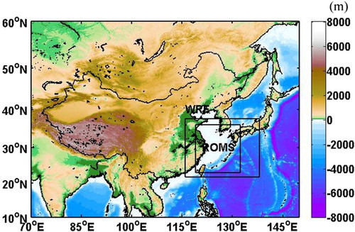
The ROMS domain (the inner box in Fig. 1) is a rectangular grid with a horizontal grid spacing of 1/24°; ROMS utilizes 32 stretched terrain-following vertical levels and its boundary conditions are specified with values from the 1/12° global HYbrid Coordinate Ocean Model (HYCOM) with Naval Research Laboratory Coupled Ocean Data Assimilation (HYCOM/NCODA) products. HYCOM assimilates satellite sea surface height and SST as well as in situ observations from expendable bathythermographs (XBTs), shipboard conductivity-temperature-depth (CTD) sensors and Argo floats (Chassignet et al., 2007). The radiation-nudging boundary condition (Marchesiello, McWilliams, & Shchepetkin, 2001), which has a time-scale of 0.5 days on inflow and 10 days on outflow, is used for ROMS tracers (salinity and temperature) and three-dimensional velocity fields. Because the free-surface boundary condition is the clamped boundary condition, Flather’s (1976) method was adopted and updated every day for depth-averaged velocity boundary conditions. A generic length scale scheme introduced to ROMS by Warner, Sherwood, Arango, and Signell (2005) was used for vertical turbulent mixing, as well as a quadratic drag formulation for the bottom friction specification.

c Coupling

Coupling the WRF and ROMS models is accomplished using the Model Coupling Toolkit, which is a fully parallelized system that uses a message passing interface to exchange model state variables. The interaction of ocean and atmospheric models occurs with momentum and heat fluxes. The sea surface momentum and heat fluxes for the ROMS are computed by the WRF model in the same way as in Warner et al. (2010). This approach assures consistent momentum and heat flux exchanges between the atmosphere and ocean. Moreover, the ocean model provides SST to the atmospheric model.

3 Results

a Model validation

In order to validate the COAWST model performance over our study area, we define two variables: bias and root mean square error (RMSE). Bias is a way of measuring the mean error in the model and can indicate whether the model tends to produce over- or underestimated values with respect to observations (Pennelly & Reuter, 2017).(1) where N is the number of grids, i denotes the ith grid in the domain, x_{m i} is the model output at grid i , and x_{obs i} is the observation at grid i. The RMSE can provide further information about the spread in error size.(2)

The Operational Sea Surface Temperature and Sea Ice Analysis (OSTIA) product (Donlon et al., 2012; National Centre for Ocean Forecasting, 2013) was used for the validation of model SST and has a resolution of 0.05° × 0.05°. The dataset used for comparison of 10 m wind speed is from the Advanced Scatterometer (ACSAT; International Pacific Research Center, 2013). To facilitate comparison, the OSTIA, ACSAT, and WRF outputs are all bilinearly interpolated onto the 1/24° ROMS grid.

Accurate representation of the wind field and SST is also important because of their potential importance in determining the air–sea interaction in the ECS. Figure 2 shows the annual mean SST and 10 m wind speed for both observations and the coupled simulation. Overall, SSTs simulated by the coupled experiment are consistent with satellite-derived SSTs. Compared with the OSTIA data, the model-simulated annual mean SST is a little lower. From the maps of 10 m wind speed (Figs 2c and 2d), we can see that the wind speed over the Yangtze River estuary is much higher for ASCAT, implying that the model underestimates the speed there. However, compared with ASCAT, the model overestimates the mean 10 m wind speed in the domain. Table 1 displays the monthly mean bias and RMSE in the coupled model. We can see that the model bias is negative from April to September, which means that SST is underestimated. However, the model overestimates SST in winter. As for the 10 m wind speed, it is overestimated in most months except winter.

Fig. 2 Annual mean SST (°C) from (a) OSTIA and (b) the coupled model. Annual mean wind speed (m s⁻¹; shading indicates the wind magnitude) from (c) ASCAT and (d) the coupled model.

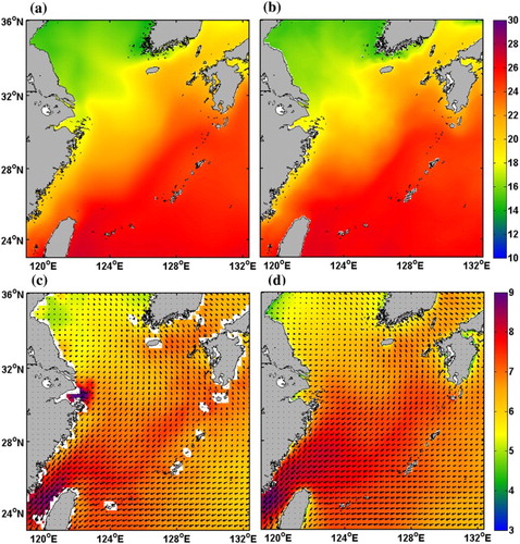
Table 1. Monthly mean values of bias and RMSE from the coupled model.

		Jan.	Feb.	Mar.	Apr.	May	Jun.	Jul.	Aug.	Sep.	Oct.	Nov.	Dec.
SST (°C)	bias	0.01	0.32	0	−0.12	−0.62	−0.24	−0.58	−0.12	−0.09	0.40	0.15	0.05
	RMSE	1.04	1.09	1.28	1.12	1.31	1.04	1.43	1.00	1.19	0.91	0.90	0.95
Wind (m s^−1)	bias	−0.24	−0.04	−0.01	0.04	0.65	0.63	0.66	0.82	0.32	0.07	−0.30	−0.28
	RMSE	1.77	1.87	1.89	1.98	2.09	2.30	1.67	2.02	2.06	1.91	1.81	1.69

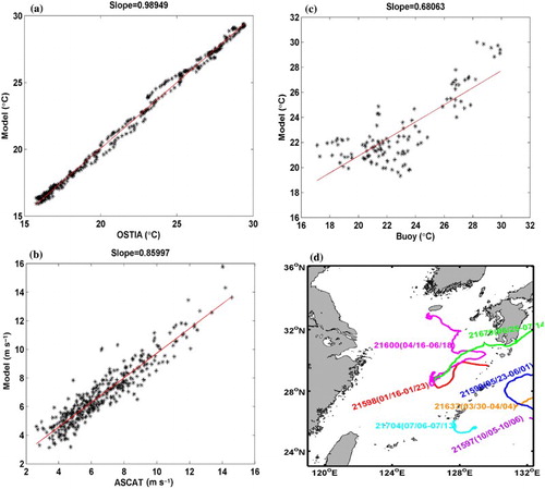
Next, we compare the daily mean fields. Figure 3a displays the scatterplots of daily mean observed and modelled SSTs. The red curve, which also gives the slope, is obtained by using a least-squares fitting method. On average, the slope is 0.98, which means that the model simulates SST well. For the 10 m wind speed, the magnitude of the slope is 0.85 (Fig. 3b), indicating that the coupled model simulates the 10 m wind speed poorly compared with SST. This weakness in the simulation of the wind speed is likely caused by the systematic biases of the WRF model in the simulation of wind speed in the lower layers. Shimada, Ohsama, Chikaoka, and Kozai (2011) used seven PBL parameterization schemes to simulate wind speed in the lower layers for one month and found that all the simulations had positive biases and that different schemes produced no obvious differences. These results also agree with Akylas, Kotroni, and Lagouvardos (2007) and Borge, Alexandrov, del Vas, Lumbreras, and Rodriguez (2008). The SST-induced wind response was assessed by Perlin et al. (2014) using eight simulations with different PBL parameterization schemes and validated using Quick Scatterometer (QuikSCAT) winds and satellite-based SSTs. Although different PBL mixing parameterization schemes have different coupling coefficients, all of them can reproduce the positive correlations of local surface wind anomalies with SST anomalies at oceanic mesoscales. Moreover, with the exception of the Grenier-Bretherton-McCaa (GBM) PBL scheme (Bretherton, McCaa, & Grenier, 2004), the YSU PBL scheme performed best. Nevertheless, the conclusions will not be affected.We also selected seven drifting buoys (21637, 21598, 21599, 21600, 21597, 21679, and 21704) within the domain during the simulation period from the Japan Meteorological Agency (JMA, 2013) to compare the SSTs. Their trajectories and durations are displayed in Fig. 3d. Although the slopes are smaller than the satellite-derived SSTs, the correlation coefficient between modelled SSTs and buoy SSTs (Fig. 3c) is 0.81(exceeding the 99% confidence level).

Fig. 3 Comparison of (a) OSTIA and coupled model SST (°C); (b) ASCAT 10 m wind speed and coupled model wind speed (m s⁻¹), and (c) buoy and coupled model SST (°C); the red line shows the linear fit. The trajectories of the different buoys are plotted in (d) using different colours for each buoy. Their corresponding IDs and durations are also displayed.

b General patterns of SST and surface wind

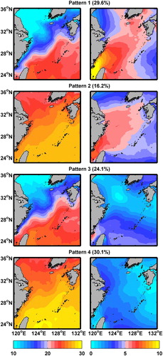
The classification of SST and surface wind is based on SOM, also known as a Kohonen map (Kohonen, 1982). SOM is an unsupervised artificial neural network that reduces a high-dimensional dataset into a low-dimensional one and summarizes the key aspects of the larger dataset into a set of patterns. Details of the approach can be found in Cassano, Uotila, and Lynch (2006). SOM has been shown to be more powerful than conventional methods (e.g., an empirical orthogonal function) in extracting consistent features (e.g., Liu, Weisberg, & Moors, 2006; Reusch, Alley, & Hewitson, 2005) and has been successfully applied in climate research (e.g., Morioka, Tozuka, & Yamagata, 2010; Shan, Guan, & Huang, 2014, 2017). A SOM algorithm produces coherence patterns of SST and surface wind. After testing several different sizes, the final shape of the Kohonen map chosen for the current study is a 2 × 2 matrix of coherence patterns that can cover most features and ensure that each pattern can provide robust statistics for the properties of the joint SST and surface wind pattern. Figure 4 shows the combined patterns of SST and surface wind and their frequencies of occurrence. Although all patterns are approximately equally distributed, Pattern 4 appears most frequently (31.1%), and Pattern 2 occurs least frequently (24.1%). In Pattern 2 and Pattern 4, the SST is in a warmer phase. However, the surface wind in Pattern 2 is much stronger than that in Pattern 4; the maximum surface wind occurs over the Taiwan Strait and the wind speed in the ECS is also much larger than in the other regions. The wind speed is much lower in Pattern 4, with a minimum wind speed centre observed near the Yangtze River estuary. In Pattern 1 and Pattern 3, the SST displays a typical northwest–southeast distribution and decreases from the Kuroshio toward the northwest ECS. Wind speed in Pattern 1 is the highest of the four patterns, and the wind speed pattern is very similar to that of Pattern 2. In Pattern 3, the wind speed displays a north–south distribution, and the wind in the north is much higher.

Fig. 4 Combined SST and surface wind patterns from a self-organizing map (SOM) with frequencies of occurrence showing SST (°C; left) and surface wind SOM (m s⁻¹; right).

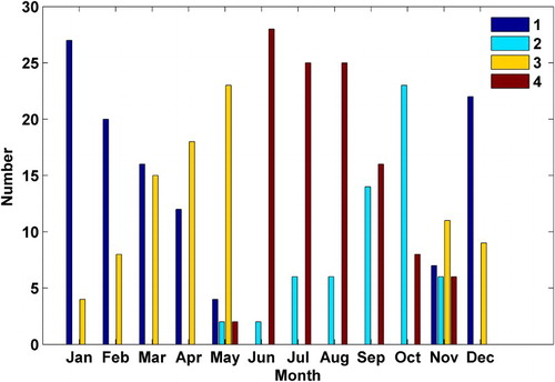
The number of occurrences of the four SST–wind patterns in each month is given in Fig. 5. Pattern 1 appears most frequently in winter, especially in December and January. Pattern 3 happens mostly in spring; it has a maximum frequency of occurrence in May. Pattern 2 and Pattern 4 occur mainly in the summer half year (from April to October), with a maximum frequency of occurrence in October and June, respectively.

Fig. 5 Distribution of occurrences of the four SST–wind patterns in each month.

c General features of SST and surface wind on different spatial scales

To show different spatial scale features of SST and surface wind, a two-dimensional spatial high-pass filter was applied to separate mesoscale signals from large-scale signals. The filter used was the quadratic loess smoother developed by Cleveland and Devlin (1988). It is based on locally weighted quadratic regression. Wind speed and SST were processed using a two-dimensional loess high-pass filter that has an elliptical window with a half span of 10° × 10°. The high-pass-filtered fields are referred to here as perturbations.

On a basin scale, the correlation between SST and surface wind is often negative (Liu, Zhang, & Bishop, 1994; Mantua, Hare, Zhang, Wallace, & Francis, 1997; Okumura, Xie, Numaguti, & Tanimoto, 2001). It is interpreted as evidence that the atmosphere drives the ocean. Figures 6 and 7 display the spatial distributions of large-scale SST and 10 m wind speed, respectively, for each month. Because of the influence of the Kuroshio in the ECS, the SST presents a northwest–southeast distribution, decreasing from the Kuroshio toward the northwest ECS. From December to April, the most evident feature is the Kuroshio SST front in the ECS. From winter to spring, this oceanic SST front gradually strengthens; the intensity of the SST front quickly decreases after May. The Yellow Sea and ECS ocean fronts are weakest in summer and the intensity of the oceanic front begins to recover gradually after October. The strength of the Kuroshio temperature front is strongest in spring and weakest in summer.

Fig. 6 Spatial distribution of large-scale modelled SST (°C) for each month.

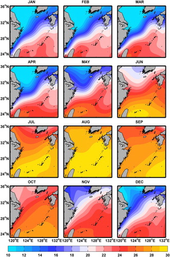
Fig. 7 As in Fig. 6 but for 10 m wind speed (m s⁻¹).

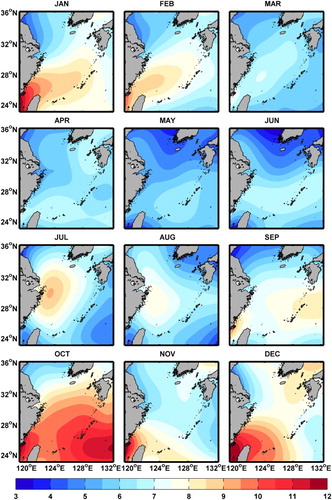
Local high wind maxima in winter are mainly located over the Taiwan Strait and over the eastern part of Taiwan Island. When the prevailing northeast winter monsoon passes through the Taiwan Strait, high winds form extremely easily because of canalization (Xu & Xu, 2013). Wind speed thus reaches its threshold in the strait. The magnitude of surface winds in spring drops drastically in the entire domain relative to that in winter. The occurrence of high winds in the Taiwan Strait and adjacent areas of Taiwan Island decreases but remains frequent. From January to March, SST fronts strongly modulate the local occurrence of high winds. In particular, frequent high wind events are observed over the warm Kuroshio as it flows along the outer edge of the continental shelf in the ECS from Taiwan to southern Japan. Variation in SST over an oceanic frontal zone will influence the surface wind velocity through its effect on atmospheric stability and vertical mixing of momentum (Chelton et al., 2001; Wallace, Mitchell, & Deser, 1989). Near the Kuroshio SST front, surface air temperature is not in equilibrium with SST, which results in an unstable atmosphere on the warmer flank of the front with strong turbulent mixing that conveys stronger winds from aloft, accelerating the surface wind and vice versa. A high wind frequency maximum no longer exists in the Taiwan Strait, and its occurrence gradually increases from south to north. The high wind area is mainly located in the region near the Yangtze River estuary. The influence of the Kuroshio SST front on surface winds weakens in summer, which indicates the reduced effect of vertical mixing on surface wind speed as the SST front relaxes in summer. The spatial distribution of surface wind is similar to that in winter, except that the high wind near the Taiwan Strait is not evident.

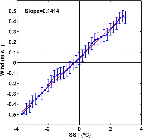
The spatially high-pass filtered SST fields for each month are shown in Fig. 8 as contours overlaid on spatially high-pass filtered 10 m wind speed. It can be seen that in the ECS warmer (colder) SSTs correspond to higher (lower) wind speeds, which is evident from January to May when the Kuroshio SST front is stronger. Consistent with previous studies, wind speed perturbations on the frontal scale are linearly related to and positively correlated with SST perturbations (Chelton & Xie, 2010; O’Neill, Esbensen, Thum, Samelson, & Chelton, 2010; Song, Chelton, Esbensen, Thum, & O’Neill, 2009). Surface wind increases over warm water in association with decreased stability through enhanced vertical mixing resulting in momentum flux from the upper boundary layer down to the sea surface. The mesoscale responses of surface winds to SST is stronger in the cold season, which is in agreement with the results of Ma, Xu, and Dong (2016) in the Kuroshio Extension region. They attribute the responses to the different background atmospheric stability during different seasons. Because the marine atmospheric boundary layer (MABL) is relatively unstable in winter and stable in summer, vertical mixing is closely related to the stability. The stronger vertical momentum mixing in winter than in summer contributes greatly to the stronger wind speed response in winter than in summer. Figure 9 shows the scatterplot of 10 m wind speed perturbations binned by the values of SST perturbations for five-month averages (January-February-March-April-May). The slope of the straight red line indicates the amount of change in wind speed per unit SST variation and serves as an indicator of the strength of the air–sea coupling. Basically, the coupling strength is about 0.14 m s⁻¹ °C, which is only half that in the Kuroshio Extension region (Ma et al., 2015).

Fig. 8 Maps of spatially high-pass-filtered SST (°C) overlaid as contours on spatially high-pass-filtered 10 m wind speeds (m s⁻¹). Positive and negative high-pass filtered SSTs are shown as red solid and black dotted lines, respectively, with a contour interval of 1°C. Zero contours are omitted for clarity.

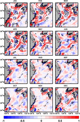
Fig. 9 Scatterplots of the spatially high-pass-filtered 10 m wind speed binned by value of SST perturbations for five-month averages (January-February-March-April-May) within the domain. The stars and error bars in the binned scatterplots are the overall average and the standard deviation of the individual binned averages, respectively. The red line shows the linear fit.

d SST and surface wind interaction

In order to investigate the interaction between SST and surface wind, we applied SVD to both SST (left field) and 10 m wind speed (right field). This technique searches for modes that explain the mean-squared temporal covariance between the two fields as much as possible (Bretherton, Smith, & Wallace, 1992). The SVD of the covariance matrix of wind speed and SST fields results in two matrices of singular vectors and one set of singular values. Each singular vector pair describes spatial patterns for each field, which have overall covariance given by the corresponding singular value. The correlation between the value of each grid point of one field and the temporal expansion value of the other field results in a heterogeneous correlation map. In our application, the pattern shown by the heterogeneous correlation map for the kth SVD expansion mode indicates the strength of the wind speed (SST) relative to the kth expansion coefficient of SST (wind speed). Table 2 gives the percentage of the squared covariance explained by the first 10 pairs of patterns. We can see that the first two modes capture more than 96% of the joint variance for both fields. Therefore, only the first two patterns are shown.

Table 2. Percentage of squared covariance explained by the first 10 pairs of patterns.

Pattern	1	2	3	4	5	6	7	8	9	10
Percentage	83.54	15.17	0.53	0.26	0.17	0.09	0.06	0.03	0.02	0.02

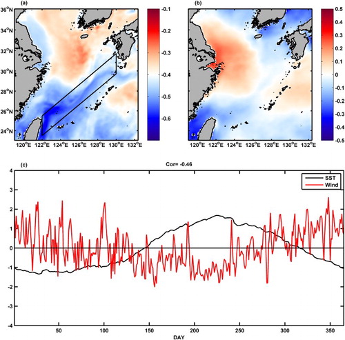
Figure 10 shows the heterogeneous correlation maps for the first mode. The left heterogeneous correlation map (Fig. 10a) indicates that the surface wind has a negative correlation with SST, especially in the Kuroshio. In the right heterogeneous correlation map (Fig. 10b), the SST in most of the ECS has a higher positive correlation with the surface wind. The corresponding time coefficient series of the two variables (Fig. 10c) for the first mode has a correlation coefficient of −0.46 (exceeding the 99% confidence level).

Fig. 10 Left (a) and right (b) heterogeneous correlation, and (c) left and right time coefficient series for the first mode.

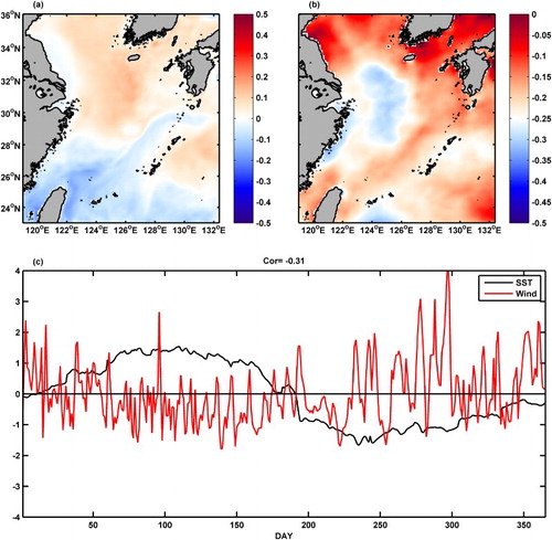
Figure 11 shows the heterogeneous correlation maps for the second mode. The negative correlation near the Kuroshio still exists in the left correlation map (Fig. 11a), but the magnitude is much smaller than that in the first mode. In addition, there is a positive correlation in many parts of the domain. It displays a negative correlation in the entire domain, especially near the Yangtze River estuary in the right correlation map (Fig. 11b). The second mode has a correlation coefficient of −0.31 (exceeding the 99% confidence level) for the two variables.

Fig. 11 As in Fig. 10 but for the second mode.

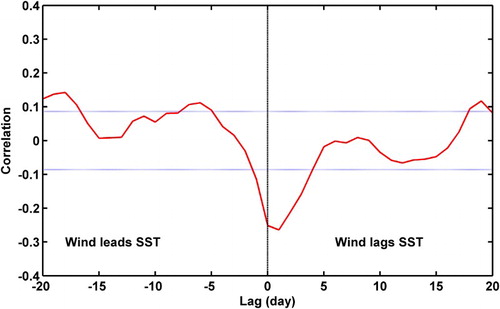
To obtain more insight into the temporal evolution of the anomaly patterns described above, we now present sequences of lagged regression patterns between the 1st principal component (PC) of SST and surface wind SVD (Fig. 12). In order to focus on short time-scales, the time coefficient series for the first modes on the left and right are filtered using a Lanczos high-pass filter with a 90-day cut-off, thereby removing seasonal and longer time-scales (note that the use of a shorter cut-off of 60 days does not change the results significantly). The negative values in Fig. 12 indicate that wind leads SST, while positive values indicate that wind lags SST. A correlation of about 0.1 is found at a lag of −6, implying that anomalously strong (weak) winds lead a maximum negative (positive) SST anomaly when the wind leads the SST by six days. A negative correlation (about −0.3) is also found around lag 1, meaning that colder (warmer) SSTs lead a weakening (strengthening) of the wind by a few days (minimum at lag 1). This could correspond to a negative feedback between SST and wind fluctuations at short time-scales.

Fig. 12 Lead-lag correlations (red line) between the 1st PC of the SVD for SST and surface wind. Correlations within the blue lines are significant at the 95% confidence level.

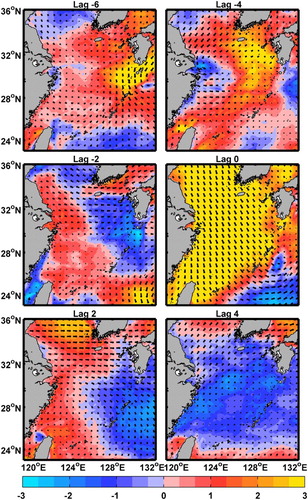
Lagged regression is a useful way to preliminarily resolve causes and consequences inside an ocean–atmosphere coupling phenomenon. It can be seen from Fig. 10a that SST and surface wind have a maximum correlation over the ECS Kuroshio (ECSK, the black box in Fig. 10a). In order to study SST and surface wind interaction, we projected surface wind anomaly fields onto the mean ECSK SST anomaly (the black box in Fig. 10a). We computed a simple correlation at each grid point between the lagged anomalous wind and the ECSK SST, weighted by the SST anomaly field. We chose to present the anomalous patterns that are linearly correlated with a negative one standard deviation of the ECSK SST anomaly (which amounts to about 0.5°C) as shown in Fig. 13. When the wind leads the SST by six days, the surface wind anomaly is significantly correlated with a cold SST anomaly. When the SST leads the wind by two days, the wind speed decreases compared with that at lag 0. From lags 2 to 6 the surface wind continues to decrease. Anomalous strong northerlies induce a cooling of the ocean within six days. This cold SST anomaly can slow the wind, thereby creating a reversed wind anomaly. These anomalous southerlies bring warmer water back to the north, resulting in the damping of the initial cold anomaly within five to six days. As the wind blows from west to the east, a warm SST anomaly appears behind the cold anomaly along the ECSK. It creates weak anomalous southerlies, which may display biweekly variability.

Fig. 13 Lagged regressions of anomalous 10 m wind fields (m s⁻¹) onto the ESCK SST anomaly. Vectors denote wind direction, and shading indicates the wind magnitude.

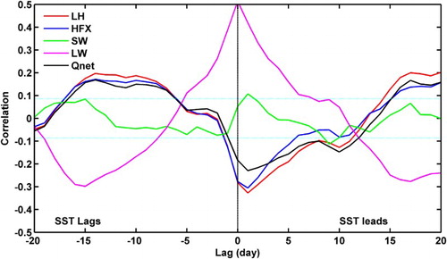
Air–sea heat fluxes are known to play an important role in causing SST fluctuations based on lead-lag analyses (He & Wu, 2013; Liu, Jiang, Xie, & Liu, 2004; Sui, Xie, & Wang, 2012; Wu, 2010; Xie, Chang, Xie, & Wang, 2007; Zhang, Wang, Xia, & Zeng, 2012). The seasonal SST variation in the South China Sea is primarily determined by the net heat flux, especially the latent heat flux because wind speed determines the latent heat flux, which is a significant factor influencing SST variation (Liu & Xie, 1999). Wu (2010) investigated intraseasonal variations of SST, wind, and heat fluxes in the South China Sea and found that intraseasonal SST changes are mainly induced by wind anomalies and rainfall anomalies and that large SST changes may also feed back to the atmosphere. In order to estimate the respective parts of the latent and sensible heat fluxes (LH and HFX, respectively), the longwave and shortwave radiation in the intraseasonal forcing of the Kuroshio SST variability, the corresponding data are averaged over the ECSK region. No significant correlation at a lag of −6 and 1 was found in the lagged cross-correlation between the ECSK SST and the longwave or shortwave radiation (Fig. 14). A significant negative correlation (about −0.35) between LH and the ECSK SST was observed when the latter lagged the heat flux by one day, which corresponds to a negative correlation when SST led wind by one day (Fig. 10). However, there is no significant correlation when SST lagged wind by five to six days. Similar results to the LH were obtained for the HFX. In the ECS, the intraseasonal SST variability is not determined by the heat flux.

Fig. 14 Lagged cross-correlations between ESCK SST and heat flux terms. The cyan lines indicate the 95% confidence level. Qnet: net surface heat flux, SW: surface solar radiation, LH: surface latent heat flux, HFX: surface sensible heat flux, and LW: surface longwave radiation.

The physical processes that lead to different SSTs were examined using the mixed-layer (ML) heat budget analysis. The vertically averaged ML heat budget equation is derived from the conservation of mass and heat equations (e.g., Moisan & Niiler, 1998; Stevenson & Niiler, 1983) and is expressed as(3) From left to right, the terms represent the ML temperature tendency, horizontal advection (Qa), entrainment (Qe), the combination of net atmospheric heating (Q_h) and residual (Res). In Eq. (3), h is ML depth; T and v are the temperature and velocity, respectively, vertically averaged from the surface to a depth of −h; T′ and v′ are deviations from the time means; T_−h is the temperature at the base of the ML; Q_net is the net surface heat flux term; ρ is the density of seawater, and c_p is the heat capacity of seawater; w_e is the entrainment velocity which is defined following Stevenson and Niiler (1983).(4) In Eq. (3) Q_−h is the downward radiative flux across the ML base, which is calculated following the empirical formula of Paulson and Simpson (1977).(5) where Q_r is the shortwave radiation flux.

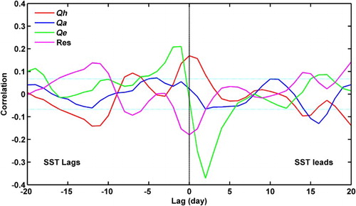
The temporal evolution of wind–SST interaction is also examined locally through the lagged regression of three main terms of the oceanic ML heat budget and SST averaged over the ECSK box (Fig. 15). Clearly, the net atmospheric heating (red line) and entrainment (green line) do not contribute much to the evolution of the SST anomaly. On the other hand, although the horizontal advection term leads the SST anomaly by about five days, there is a positive correlation of about 0.1, and there is a negative correlation when the SST anomaly leads the horizontal advection term by two days. This indicates the contribution of horizontal advection in determining these intraseasonal SST signals.

Fig. 15 Lagged cross-correlations between mean mixed-layer (ML) temperature in the ECSK and the main terms of the local ML heat budget. The cyan lines indicate the 90% confidence level.

4 Summary

In order to study the interaction between SST and surface wind in the ECS, we used a regional coupled ocean–atmosphere model of COAWST to downscale a global atmospheric reanalysis product over the ECS in 2013. We first validated the coupled model outputs by comparing the simulated SST and wind speed fields with satellite observations, which indicates the ability of the coupled model to reproduce the observed surface wind and SST with the primary spatial and temporal features of SST and surface wind captured. An SVD was applied to the SST and surface wind speed to study their coupling relationship. The heterogeneous correlation map indicates that the surface wind has a negative correlation with the SST, especially in the Kuroshio. From lead-lag correlations between the 1st PC of SST and surface wind SVD, a correlation of about 0.1 was found at a lag of −6, implying that anomalously strong (weak) winds lead to a maximum negative (positive) SST anomaly when the wind leads SST by six days. A negative correlation of about −0.3 is also found around lag 1, meaning that colder (warmer) SSTs lead to the weakening (strengthening) of the wind by a few days (minimum at lag 1). This could indicate a negative feedback between SST and wind fluctuations at short time-scales. Air–sea heat fluxes are known to play an important role in SST fluctuations. We calculated the lead-lag correlation between the net heat flux and ECSK SST and found that the net heat flux seems to contribute little to the ECSK SST variability.

The physical processes that lead to different SST patterns were also examined using an ML heat budget analysis. The leading factor is the advection of mean SST by an anomalous crossing of the Kuroshio forced by anomalous winds at short time-scales. In summary, around the ECSK, anomalous strong winds are followed by the cooling of the ocean surface within five days, mainly through the southward advection of the surface water near the ECSK and, to a smaller extent, through the anomalous vertical mixing and air–sea fluxes. Further, the cold SST anomaly slows the wind, thereby creating a reversed wind anomaly, which reaches a maximum after two to three days. The mechanism involved in this reversal is clearly linked to the vertical adjustment of the MABL stability, although the sea level pressure gradient induced by the SST gradient could also play an important role. These anomalous southerlies bring warmer water back to the north, resulting in the damping of the initial cold anomaly within five to six days. As the mean current advects the centre of the cold anomaly eastward, a warm SST anomaly appears behind the cold anomaly along the ECSK; it creates weak anomalous southerlies, which may support the biweekly variability.

Acknowledgements

The authors wish to thank the science editor and two anonymous reviewers for their valuable comments and suggestions, which helped enhance the manuscript considerably.

Disclosure statement

No potential conflict of interest was reported by the authors.

Additional information

Funding

This work was supported by the National Natural Science Foundation of China (NSFC) [grant number 41606023], the Natural Science Foundation of Jiangsu Province [grant number BK20150912], China Postdoctoral Science Foundation funded project [grant number 2015M581834], NSFC [grant number 41476022] and [grant number 41490643], the Startup Foundation for Introducing Talent, Nanjing University of Information Science and Technology [grant number 2013r121] and [grant number 2014r072], the Program for Innovation Research and Entrepreneurship team in Jiangsu Province, National Programme on Global Change and Air-Sea Interaction [grant number GASI-IPOVAI-05], The National Key Research Program of China [grant number 2016YFA0601803], and the Priority Academic Program Development of Jiangsu Higher Education Institutions (PAPD).

References

- Akylas, E., Kotroni, V., & Lagouvardos, K. (2007). Sensitivity of high-resolution operational weather forecasts to the choice of the planetary boundary layer scheme. Atmospheric Research, 84(1), 49–57. doi: 10.1016/j.atmosres.2006.06.001
- Borge, R., Alexandrov, V., del Vas, J. J., Lumbreras, J., & Rodriguez, E. (2008). A comprehensive sensitivity analysis of the WRF model for air quality applications over the Iberian Peninsula. Atmospheric Environment, 42(37), 8560–8574. doi: 10.1016/j.atmosenv.2008.08.032
- Bretherton, C. S., McCaa, J. R., & Grenier, H. (2004). A new parameterization for shallow cumulus convection and its application to marine subtropical cloud-topped boundary layers. Part I: Description and 1D results. Monthly Weather Review, 132, 864–882. doi: 10.1175/1520-0493(2004)132<0864:ANPFSC>2.0.CO;2
- Bretherton, C. S., Smith, C., & Wallace, J. M. (1992). An intercomparison of methods for finding coupled patterns in climate data. Journal of Climate, 5, 541–560. doi: 10.1175/1520-0442(1992)005<0541:AIOMFF>2.0.CO;2
- Bryan, F. O., Tomas, R., Dennis, J., Chelton, D. B., Loeb, N. G., & McClean, J. L. (2010). Frontal scale air-sea interaction in high-resolution coupled climate models. Journal of Climate, 23, 6277–6291. doi: 10.1175/2010JCLI3665.1
- Byrne, D., Papritz, L., Frenger, I., Munnich, M., & Gruber, N. (2015). Atmospheric response to mesoscale sea surface temperature anomalies: Assessment of mechanisms and coupling strength in a high resolution coupled model over the South Atlantic. Journal of the Atmospheric Sciences, 72, 1872–1890. doi: 10.1175/JAS-D-14-0195.1
- Cassano, J. J., Uotila, P., & Lynch, A. (2006). Changes in synoptic weather patterns in the polar regions in the twentieth and twenty-first centuries, part 1: Arctic. International Journal of Climatology, 26, 1027–1049. doi: 10.1002/joc.1306
- Chassignet, E. P., Hurlburt, H. E., Smedstad, O. M., Halliwell, G. R., Hogan, P. J., Wallcraft, A. J., … Bleck, R. (2007). The HYCOM (Hybrid Coordinate Ocean Model) data assimilative system. Journal of Marine Systems, 65, 60–83. doi: 10.1016/j.jmarsys.2005.09.016
- Chelton, D., Esbensen, S., Schlax, M., Thum, N., Freilich, M., Wentz, F., … Schopf, P. (2001). Observations of coupling between surface wind stress and sea surface temperature in the eastern tropical Pacific. Journal of Climate, 14, 1479–1498. doi: 10.1175/1520-0442(2001)014<1479:OOCBSW>2.0.CO;2
- Chelton, D., Schlax, M., & Freilich, M. (2004). Satellite measurements reveal persistent small-scale features in ocean winds. Science, 303, 978–983. doi: 10.1126/science.1091901
- Chelton, D., & Xie, S. P. (2010). Coupled ocean-atmosphere interaction at oceanic mesoscales. Oceanography, 23(4), 52–69. doi: 10.5670/oceanog.2010.05
- Chen, D., Liu, W. T., Tang, W., & Wang, Z. (2003). Air-sea interaction at an oceanic front: Implications for frontogenesis and primary production. Geophysical Research Letters, 30(14), 335. doi: 10.1029/2003GL017536
- Cleveland, W. S., & Devlin, S. J. (1988). Locally weighted regression: An approach to regression analysis by local fitting. Journal of the American Statistical Association, 83, 596–610. doi: 10.1080/01621459.1988.10478639
- Deng, J., & Xu, H. (2016). Nonlinear effect on the East Asian summer monsoon due to two coexisting anthropogenic forcing factors in eastern China: An AGCM study. Climate Dynamics, 46, 3767–3784. doi: 10.1007/s00382-015-2803-y
- Dong, C., McWilliams, J., Liu, Y., & Chen, D. (2014). Global heat and salt transports by eddy movements. Nature Communications, 5, 3294. doi: 10.1038/ncomms4294
- Donlon, C. J., Martin, M., Stark, J. D., Roberts-Jones, J., Fiedler, E., & Wimmer, W. (2012). The operational sea surface temperature and sea ice analysis (OSTIA) system. Remote Sensing of Environment, 116, 140–158. doi: 10.1016/j.rse.2010.10.017
- Dudhia, J. (1989). Numerical study of convection observed during the winter monsoon experiment using a mesoscale two-dimensional model. Journal of the Atmospheric Sciences, 46, 3077–3107. doi: 10.1175/1520-0469(1989)046<3077:NSOCOD>2.0.CO;2
- Fang, Y., Zhang, Y., Tang, J., & Ren, X. (2010). A regional air-sea coupled model and its application over East Asia in the summer of 2000. Advances in Atmospheric Sciences, 27, 583–593. doi: 10.1007/s00376-009-8203-7
- Flather, R. A. (1976). A tidal model of the northwest European continental shelf. Memoires Societe Royale des Sciences de Liege, 6, 141–164.
- Frenger, I., Gruber, N., Knutti, R., & Münnich, M. (2013). Imprint of Southern Ocean eddies on winds, clouds and rainfall. Nature Geoscience, 6(8), 608–612. doi: 10.1038/ngeo1863
- Gaube, P., Chelton, D. B., Samelson, R. M., Schlax, M. G., & O’Neill, L. W. (2015). Satellite observations of mesoscale eddy-induced Ekman pumping. Journal of Physical Oceanography, 45, 104–132. doi: 10.1175/JPO-D-14-0032.1
- Haack, T., Chelton, D., Pullen, J., Doyle, J. D., & Schlax, M. (2008). Summertime influence of SST on surface wind stress off the U.S. West Coast from the U.S. Navy COAMPS model. Journal of Physical Oceanography, 38, 2414–2437. doi: 10.1175/2008JPO3870.1
- Haidvogel, D. B., Arango, H. G., Budgell, W. P., Cornuelle, B. D., Curchitser, E., Di Lorenzo, E., … Wilkin, J. (2008). Ocean forecasting in terrain-following coordinates: Formulation and skill assessment of the Regional Ocean Modeling System. Journal of Computational Physics, 227, 3595–3624. doi: 10.1016/j.jcp.2007.06.016
- He, Z. Q., & Wu, R. G. (2013). Coupled seasonal variability in the South China Sea. Journal of Oceanography, 69, 57–69. doi: 10.1007/s10872-012-0157-1
- Hong, S. Y., Dudhia, J., & Chen, S. H. (2004). A revised approach to ice microphysical processes for the bulk parameterization of clouds and precipitation. Monthly Weather Review, 132, 103–120. doi: 10.1175/1520-0493(2004)132<0103:ARATIM>2.0.CO;2
- International Pacific Research Center. (2013). Daily advanced scatterometer (ASCAT) surface wind fields level 3 [Dataset]. Retrieved from the Asia-Pacific Data Research Center website: http://apdrc.soest.hawaii.edu/datadoc/ascat.php
- Iwasaki, S., Isobe, A., & Kako, S. (2014). Atmosphere-ocean coupled process along coastal areas of the Yellow and East China Seas in winter. Journal of Climate, 27, 155–167. doi: 10.1175/JCLI-D-13-00117.1
- Japan Meteorological Agency. (2013). Ocean data buoy observations [Data]. Retrieved from http://www.data.jma.go.jp/gmd/kaiyou/db/vessel_obs/data-report/html/buoy/buoy_e.php?year=2013#kisetsu
- Kain, J. S. (2004). The Kain-Fritsch convective parameterization: An update. Journal of Applied Meteorology, 43, 170–181. doi: 10.1175/1520-0450(2004)043<0170:TKCPAU>2.0.CO;2
- Kohonen, T. (1982). Self-organized formation of topologically correct feature maps. Biological Cybernetics,, 43, 59–69. doi: 10.1007/BF00337288
- Li, T., & Zhou, G. Q. (2010). Preliminary results of a regional air-sea coupled model over East Asia. Chinese Science Bulletin, 55, 2295–2305. doi: 10.1007/s11434-010-3071-1
- Liu, Q. Y., Jiang, X., Xie, S. P., & Liu, W. T. (2004). A gap in the Indo-Pacific warm pool over the South China Sea in boreal winter: Seasonal development and interannual variability. Journal of Geophysical Research, 109, C07012. doi: 10.1029/2003JC002179
- Liu, W. T., Xie, X., & Niiler, P. P. (2007). Ocean-atmosphere interaction over Agulhas Extension meanders. Journal of Climate, 20, 5784–5797. doi: 10.1175/2007JCLI1732.1
- Liu, W. T., & Xie, X. S. (1999). Spacebased observations of the seasonal changes of South Asian monsoons and oceanic responses. Geophysical Research Letters, 26(10), 1473–1476. doi: 10.1029/1999GL900289
- Liu, W. T., Zhang, A., & Bishop, J. K. B. (1994). Evaporation and solar irradiance as regulators of sea surface temperature in annual and interannual changes. Journal of Geophysical Research, 99, 12623–12637. doi: 10.1029/94JC00604
- Liu, Y., Weisberg, R. H., & Moors, C. N. K. (2006). Performance evaluation of the self-organizing map for feature extraction. Journal of Geophysical Research, 111, C05018. doi: 10.1029/2005JC003117
- Ma, J., Xu, H., & Dong, C. (2016). Seasonal variations in atmospheric responses to oceanic eddies in the Kuroshio Extension. Tellus A: Dynamic Meteorology and Oceanography, 68, 31563. doi: 10.3402/tellusa.v68.31563
- Ma, J., Xu, H., Dong, C., Lin, P., & Liu, Y. (2015). Atmospheric responses to oceanic eddies in the Kuroshio Extension region. Journal of Geophysical Research, 120, 6313–6330.
- Mantua, N. J., Hare, S. R., Zhang, Y., Wallace, J. M., & Francis, R. C. (1997). A Pacific interdecadal climate oscillation with impacts on salmon production. Bulletin of the American Meteorological Society, 78, 1069–1079. doi: 10.1175/1520-0477(1997)078<1069:APICOW>2.0.CO;2
- Marchesiello, P., McWilliams, J. C., & Shchepetkin, A. F. (2001). Open boundary conditions for long-term integration of regional oceanic models. Ocean Modelling, 3, 1–20. doi: 10.1016/S1463-5003(00)00013-5
- Miyama, T., Nonaka, M., Nakamura, H., & Kuwano-Yoshida, A. (2012). A striking early-summer event of a convective rainband persistent along the warm Kuroshio in the East China Sea. Tellus A: Dynamic Meteorology and Oceanography, 64, 18962. doi: 10.3402/tellusa.v64i0.18962
- Mlawer, E. J., Taubman, S. J., Brown, P. D., Iacono, M., & Clough, J., & A, S. (1997). Radiative transfer for inhomogeneous atmospheres: RRTM, a validated correlated-k model for the longwave. Journal of Geophysical Research: Atmospheres, 102(D14), 16663–16682. doi: 10.1029/97JD00237
- Moisan, J. R., & Niiler, P. P. (1998). The seasonal heat budget of the North Pacific: Net heat flux and heat storage rates (1950–1990). Journal of Physical Oceanography, 28, 401–421. doi: 10.1175/1520-0485(1998)028<0401:TSHBOT>2.0.CO;2
- Morioka, Y., Tozuka, T., & Yamagata, T. (2010). Climate variability in the southern Indian Ocean as revealed by self-organizing maps. Climate Dynamics, 35, 1075–1088. doi: 10.1007/s00382-010-0843-x
- National Center for Atmospheric Research. (2013). NCEP climate forecast system version 2 (CFSv2) 6-hourly products [Dataset]. Retrieved from https://rda.ucar.edu/datasets/ds094.0/
- National Centre for Ocean Forecasting. (2013). Operational sea surface temperature and sea ice analysis (OSTIA). Retrieved from http://ghrsst-pp.metoffice.com/pages/latest_analysis/ostia.html
- Noh, Y., Cheon, W. G., Hong, S. Y., & Raasch, S. (2003). Improvement of the K-profile model for the planetary boundary layer based on large eddy simulation data. Boundary-Layer Meteorology, 107, 401–427. doi: 10.1023/A:1022146015946
- Nonaka, M., & Xie, S. P. (2003). Covariations of sea surface temperature and wind over the Kuroshio and its extension: Evidence for ocean-to-atmosphere feedback. Journal of Climate, 16, 1404–1413. doi: 10.1175/1520-0442(2003)16<1404:COSSTA>2.0.CO;2
- Okumura, Y., Xie, S. P., Numaguti, A., & Tanimoto, Y. (2001). Tropical Atlantic air-sea interaction and its influence on the NAO. Geophysical Research Letters, 28, 1507–1510. doi: 10.1029/2000GL012565
- O’Neill, L. W., Chelton, D. B., & Esbensen, S. K. (2003). Observations of SST-induced perturbations of the wind stress field over the southern ocean on seasonal timescales. Journal of Climate, 16, 2340–2354. doi: 10.1175/2780.1
- O’Neill, L. W., Chelton, D. B., Esbensen, S. K., & Wentz, F. J. (2005). High-resolution satellite measurements of the atmospheric boundary layer response to SST variations along the Agulhas return current. Journal of Climate, 18, 2706–2723. doi: 10.1175/JCLI3415.1
- O’Neill, L. W., Esbensen, S. K., Thum, N., Samelson, R. M., & Chelton, D. B. (2010). Dynamical analysis of the boundary layer and surface wind responses to mesoscale SST perturbations. Journal of Climate, 23, 559–581. doi: 10.1175/2009JCLI2662.1
- Paulson, C. A., & Simpson, J. J. (1977). Irradiance measurements in the upper ocean. Journal of Physical Oceanography, 7, 952–956. doi: 10.1175/1520-0485(1977)007<0952:IMITUO>2.0.CO;2
- Pegion, K., & Kirtman, B. (2008). The impact of air–sea interactions on the simulation of tropical intraseasonal variability. Journal of Climate, 21, 6616–6635. doi: 10.1175/2008JCLI2180.1
- Pennelly, C., & Reuter, G. (2017). Verification of the weather research and forecasting model when forecasting daily surface conditions in southern Alberta. Atmosphere-Ocean, 55(1), 31–41. doi: 10.1080/07055900.2017.1282345
- Perlin, N., de Szoeke, S. P., Chelton, D. B., Samelson, M., Skyllingstad, E. D., & O’Neill, L. W. (2014). Modeling the atmospheric boundary layer wind response to mesoscale sea surface temperature perturbations. Monthly Weather Review, 142, 4284–4307. doi: 10.1175/MWR-D-13-00332.1
- Ren, X., & Qian, Y. (2005). A coupled regional air-sea model, its performance and climate drift in simulation of the East Asian summer monsoon in 1998. International Journal of Climatology, 25, 679–692. doi: 10.1002/joc.1137
- Reusch, D. B., Alley, R. B., & Hewitson, B. C. (2005). Relative performance of self-organizing maps and principal component analysis in pattern extraction from synthetic climatological data. Polar Geography, 29, 188–212. doi: 10.1080/789610199
- Seo, H., Jochum, M., Murtugudde, R., Miller, A. J., & Roads, J. O. (2007). Feedback of tropical instability-wave-induced atmospheric variability onto the ocean. Journal of Climate, 20, 5842–5855. doi: 10.1175/JCLI4330.1
- Seo, H., Murtugudde, R., Jochum, M., & Miller, A. J. (2008). Modeling of mesoscale coupled ocean–atmosphere interaction and its feedback to ocean in the western Arabian Sea. Ocean Modelling, 25, 120–131. doi: 10.1016/j.ocemod.2008.07.003
- Shan, H. X., Guan, Y. P., & Huang, J. P. (2014). Surface air temperature patterns on a decadal scale in China using self-organizing map and their relationship to Indo-Pacific warm pool. International Journal of Climatology, 34, 3752–3765. doi: 10.1002/joc.3943
- Shan, H. X., Guan, Y. P., Huang, J. P., & Dong, C. M. (2017). Trajectory patterns of the annual cycle of the heat centre of the Indo-Pacific warm pool. International Journal of Climatology, 37, 637–647. doi: 10.1002/joc.4729
- Shchepetkin, A. F., & McWilliams, J. C. (2005). The regional oceanic modeling system (ROMS): A split-explicit, free-surface, topography-following-coordinate oceanic model. Ocean Modelling, 9, 347–404. doi: 10.1016/j.ocemod.2004.08.002
- Shimada, S., Ohsama, T., Chikaoka, S., & Kozai, K. (2011). Accuracy of the wind speed profile in the lower PBL as simulated by the WRF model. Scientific Online Letters on the Atmosphere, 7, 109–112.
- Shukla, R. P., & Zhu, J. (2014). Simulations of boreal summer intraseasonal oscillations with the climate forecast system, version 2, over India and the Western Pacific: Role of air–sea coupling. Atmosphere-Ocean, 52(4), 321–330. doi: 10.1080/07055900.2014.939575
- Skamarock, W.C., Klemp, J.B., Dudhia, J., Gill, D. O., Barker, M., Duda, K.G., Huang, X.Y., Wang, W., & Powers, J.G. (2008). A description of the advanced research WRF version 3 (NCAR/TN-475+STR, NCAR Technical Note). Boulder, Colorado, USA.
- Song, Q., Chelton, D. B., Esbensen, S. K., Thum, N., & O’Neill, L. W. (2009). Coupling between sea surface temperature and low-level winds in mesoscale numerical models. Journal of Climate, 22, 146–164. doi: 10.1175/2008JCLI2488.1
- Stevenson, J. W., & Niiler, P. P. (1983). Upper ocean heat budget during the Hawaii-to-Tahiti shuttle experiment. Journal of Physical Oceanography, 13, 1894–1907. doi: 10.1175/1520-0485(1983)013<1894:UOHBDT>2.0.CO;2
- Sui, D., Xie, Q., & Wang, D. (2012). A discuss on interannual to decadal variations of latent heat exchange over the South China Sea. Acta Oceanologica Sinica, 34(4), 27–34.
- Tokinaga, H., Tanimoto, Y., Nonaka, M., Taguchi, B., Fukamachi, T., Xie, S. P., … Yasuda, I. (2006). Atmospheric sounding over the winter Kuroshio Extension: Effect of surface stability on atmospheric boundary layer structure. Geophysical Research Letters, 33, L04703. doi: 10.1029/2005GL025102
- Tokinaga, H., Tanimoto, Y., & Xie, S. P. (2005). SST-induced surface wind variations over the Brazil–Malvinas confluence: Satellite and in situ observations. Journal of Climate, 18, 3470–3482. doi: 10.1175/JCLI3485.1
- Vecchi, G., Xie, S. P., & Fischer, A. (2004). Ocean-atmosphere covariability in the western Arabian Sea. Journal of Climate, 17, 1213–1224. doi: 10.1175/1520-0442(2004)017<1213:OCITWA>2.0.CO;2
- Wallace, J., Mitchell, T., & Deser, C. (1989). The influence of sea-surface temperature on surface wind in the Eastern equatorial Pacific: Seasonal and interannual variability. Journal of Climate, 2, 1492–1499. doi: 10.1175/1520-0442(1989)002<1492:TIOSST>2.0.CO;2
- Wallace, J., Smith, C., & Jiang, Q. (1990). Spatial patterns of atmosphere–ocean interaction in the northern winter. Journal of Climate, 3, 990–998. doi: 10.1175/1520-0442(1990)003<0990:SPOAOI>2.0.CO;2
- Warner, J. C., Armstrong, B., He, R., & Zambon, J. B. (2010). Development of a coupled ocean–atmosphere–wave–sediment transport (COAWST) modeling system. Ocean Modelling, 35, 230–244. doi: 10.1016/j.ocemod.2010.07.010
- Warner, J. C., Sherwood, C. R., Arango, H. G., & Signell, R. P. (2005). Performance of four turbulence closure models implemented using a generic length scale method. Ocean Modelling, 8, 81–113. doi: 10.1016/j.ocemod.2003.12.003
- Wu, R. G. (2010). Subseasonal variability during the South China Sea summer monsoon onset. Climate Dynamics, 34, 629–642. doi: 10.1007/s00382-009-0679-4
- Wu, R., & Kirtman, B. (2005). Roles of Indian and Pacific Ocean air–sea coupling in tropical atmospheric variability. Climate Dynamics, 25, 155–170. doi: 10.1007/s00382-005-0003-x
- Wu, R., Kirtman, B. P., & Pegion, K. (2006). Local air–sea relationship in observations and model simulations. Journal of Climate, 19, 4914–4932. doi: 10.1175/JCLI3904.1
- Xie, S. P. (2004). Satellite observations of cool ocean–atmosphere interaction. Bulletin of the American Meteorological Society, 85, 195–208. doi: 10.1175/BAMS-85-2-195
- Xie, S. P., Chang, C. H., Xie, Q., & Wang, D. X. (2007). Intraseasonal variability in the summer South China Sea: Wind jet, cold filament, and recirculations. Journal of Geophysical Research, 112, C10008. doi: 10.1029/2007JC004238
- Xie, S. P., Hafner, J., Tanimoto, Y., Liu, W. T., Tokinaga, H., & Xu, H. (2002). Bathymetric effect on the winter sea surface temperature and climate of the Yellow and East China Seas. Geophysical Research Letters, 29, 2228. doi: 10.1029/2002GL015884
- Xu, H., Tokinaga, H., & Xie, S. P. (2010). Atmospheric effects of the Kuroshio large meander during 2004–05. Journal of Climate, 23, 4704–4715. doi: 10.1175/2010JCLI3267.1
- Xu, M., & Xu, H. (2013). The characteristics of high wind distribution in China’s coastal region and their causes. Journal of Tropical Meteorology, 19(1), 49–58.
- Xu, H., Xu, M., Xie, S. P., & Wang, Y. (2011). Deep atmospheric response to the spring Kuroshio over the East China Sea. Journal of Climate, 24(18), 4959–4972. doi: 10.1175/JCLI-D-10-05034.1
- Xu, M., & Xu, H. (2015). Atmospheric responses to Kuroshio SST front in the East China Sea under different prevailing winds in winter and spring. Journal of Climate, 28, 3191–3211. doi: 10.1175/JCLI-D-13-00675.1
- Xu, M., & Xu, H. (2017). Influence of Kuroshio SST front in the East China Sea on the climatological evolution of Meiyu rainband. Climate Dynamics, Advance online publication. doi: 10.1007/s00382-017-3681-2
- Zhang, Y., Wang, D., Xia, H., & Zeng, L. (2012). The seasonal variability of an air-sea heat flux in the northern South China Sea. Acta Oceanologica Sinica, 31(5), 79–86. doi: 10.1007/s13131-012-0238-4