Seasonal Cycles, Hypoxia, and Renewal in a Coastal Fjord (Barkley Sound, British Columbia)

ABSTRACT

The west coast of Vancouver Island (WCVI) is an important marine ecosystem in which concentrations of dissolved oxygen can reach hypoxic levels at certain times of the year. Although the general features of its oceanography are well understood, little is known in particular about the seasonal cycle of oxygen in shelf areas and its interannual variability. It is possible that high temporal resolution monitoring efforts could be carried out relatively easily in sheltered fjords adjacent to the shelf, but the linkages between conditions in these fjords and those on the shelf are also not known. Here a 10-year time series of monthly hydrographic stations in Barkley Sound, British Columbia, is used to identify the seasonal cycle of temperature, salinity, density, dissolved oxygen, and chlorophyll fluorescence in a WCVI fjord. Analysis suggests that there is a standard estuarine circulation in surface and near-surface waters of the Sound, as well as a deep renewal cycle in intermediate and deep waters, and that the two are largely independent. The deep basin in the Sound undergoes annual summer renewals in response to wind-driven upwelling on the shelf, separated by stagnation and hypoxia during fall, winter, and spring downwelling periods. Other than for the stagnant deep waters in winter, residence times in different parts of the Sound are only a few weeks. Barkley Sound characteristics thus adjust rapidly to shelf conditions, and inshore measurements can be used with care as a proxy for some shelf properties. However, phytoplankton biomass does not appear to be affected by the onset of deep renewal and the associated reversal of along-shore winds and instead responds to local factors. Finally, once the seasonal cycle has been accounted for, interannual variations in temperature, density, and dissolved oxygen are uncoupled, possibly in response to longer-term changes in the characteristics of source waters offshore and/or to changes in shelf processes.

Résumé

[Traduit par la rédaction] La côte ouest de l’île de Vancouver est un écosystème marin important dans lequel les concentrations d’oxygène dissous peuvent s’abaisser à des niveaux hypoxiques à certains moments de l’année. Bien que ses grandes caractéristiques océanographiques soient bien comprises, il en va autrement notamment du cycle saisonnier de l’oxygène sur le plateau et de sa variabilité interannuelle. Il serait possible et relativement facile d’entreprendre des activités de surveillance à haute résolution dans les fjords abrités adjacents au plateau, mais les liens entre les conditions dans ces fjords et celles du plateau ne sont pas connus non plus. Nous utilisons ici une série temporelle mensuelle de dix ans issue des stations hydrographiques de la baie Barkley (Colombie-Britannique), afin de déterminer le cycle saisonnier de la température, de la salinité, de la densité, de l’oxygène dissous et de la fluorescence chlorophyllienne dans un fjord de la côte ouest de l’île de Vancouver. Les analyses laissent penser qu’il existe une circulation estuarienne normale des eaux de la baie en surface et près de la surface, ainsi qu’un cycle profond de renouvellement des eaux intermédiaires et profondes, et que ces deux processus restent indépendants. Le bassin profond de la baie est l’objet de renouvellements annuels estivaux en réaction à la remontée des eaux due au vent sur le plateau, suivis de stagnation et d’hypoxie durant la plongée des eaux en automne, en hiver et au printemps. Sauf pour les eaux profondes stagnantes en hiver, le temps de résidence de l’eau dans les différentes portions de la baie n’est que de quelques semaines. Les conditions dans la baie de Barkley s’ajustent donc rapidement aux conditions du plateau. Conséquemment, nous pouvons utiliser sous réserve les mesures prises près de la côte pour déterminer certaines propriétés du plateau. Toutefois, la biomasse du phytoplancton ne semble affectée ni par les renouvellements de l’eau profonde ni par les renversements associés au vent soufflant le long de la côte, elle réagit plutôt aux facteurs locaux. Finalement, une fois le cycle saisonnier écarté, les variations interannuelles de température, de densité et d’oxygène dissous ne restent pas couplées, possiblement en réaction aux changements à long terme des caractéristiques des eaux sources du large ou de la modification des processus du plateau.

KEYWORDS:

• Barkley sound
• oxygen
• circulation
• seasonal
• interannual

1 Introduction

The west coast of Vancouver Island (WVCI; Fig. 1), British Columbia, Canada, is a highly productive marine ecosystem that supports large and important fisheries (McFarlane, Ware, Thomson, Mackas, & Robinson, 1997). In some offshore and neighbouring coastal waters it has been observed that levels of dissolved oxygen have been dropping in recent years and that intermittent hypoxic events are becoming more frequent and covering a larger area (Connolly, Hickey, Geier, & Cochlan, 2010; Peterson, Morgan, Peterson, & Lorenzo, 2013; Whitney, Freeland, & Robert, 2007), but it is not clear if this is the case for the WCVI. Regular surveys of the shelf occur several times a year and within-summer trends have recently been described by Crawford and Peña (2013), but there is a significant seasonality to oceanographic conditions, and the available data are not sufficiently comprehensive to fully separate seasonal variations and long-term trends.

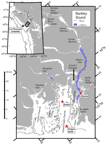
Fig. 1 Barkley Sound, British Columbia. Location of main map is shown by hatched area in inset map. A contour line is drawn at 50 m, and areas deeper than 150 m (occuring in Effingham and Alberni Inlets) are hatched. Hydrographic stations are marked with red stars, the La Perouse weather buoy with a black star, river flow gauges with red circles, and the Bamfield tide station with a red square.

Further, it is difficult to predict WCVI conditions using information about the well-studied regions on the Washington, Oregon, and California coasts further south (e.g., Connolly et al., 2010). As recently discussed in a modelling study (Bianucci, Denman, & Ianson, 2011), the biophysical and physical dynamics of the WCVI shelf region are more complicated for a number of reasons. First, the shelf is wider and its bathymetry is more complex. Second, currents and nutrient loads are partially controlled by the Vancouver Island Coastal Current, which is generated by the large seasonal freshwater outflow through nearby Juan de Fuca Strait. Third, the general climatic pattern, which governs winds, is at the boundary between the subtropical and subpolar regions (Thomson, 1981), so wind patterns are not as predictable.

However, the WCVI is heavily indented, containing a number of fjord inlets, and high temporal resolution monitoring of ocean conditions can be carried out relatively easily in these more sheltered waters. If conditions in these inlets can be related to those found offshore, inlet measurements may prove useful in characterizing shelf conditions and providing insight into the relationships between different forcing factors and WCVI hypoxia.

In addition to their possible use as proxies for offshore conditions, WCVI inlets (especially the largest, Barkley Sound) are also important for a number of scientific, commercial, industrial, and recreational purposes. The increasing number of resource conflicts between different interests in the area has recently motivated the development of a comprehensive management plan (West Coast Aquatic, 2012), whose implementation in turn requires scientific information about these inlets.

In light of their local (and possibly broader) importance, it is, therefore, surprising that very little is known about the basic oceanography of WCVI inlets. Although the general characteristics of fjord dynamical processes are well known, both in general (e.g., Farmer & Freeland, 1983; Pickard, 1963, 1975) and in this area (e.g., Farmer & Osborn, 1976; Stucchi, 1983), and the oceanography of the offshore region has been studied comprehensively in recent years (McFarlane et al., 1997), there are no published time series showing seasonal cycles of water mass characteristics within Barkley Sound or indeed any other WCVI fjord inlet. The only exception is for the permanently anoxic Nitinat Lake (Pawlowicz, Baldwin et al., 2007), which is unrepresentative of the coast. However, the detailed oceanography of these inlets can sometimes be complex, with bottom waters that are hypoxic during part of the year, and in some cases anoxic, and almost nothing is known about the interannual variability of these characteristics.

The purposes of this paper are then to quantify the seasonal cycle of temperature, salinity, density, dissolved oxygen, and primary production in Barkley Sound, to describe dynamical parameters that govern circulation, and to relate these seasonal cycles to the timing of deep and intermediate water renewals and the presence of hypoxic conditions. In addition, the interannual variability of different oceanographic characteristics will be quantified and linked to a discussion of shelf conditions. The main source of information is a monthly time series of hydrographic profiles in Barkley Sound, covering the years 2004 to 2013. This time series was augmented from late 2009 onwards by continuous near-bottom measurements at the mouth of Barkley Sound obtained from a node of the Ocean Networks Canada ocean observatory.

2 Site

Barkley Sound is a large rectangular embayment opening onto the northeast Pacific. It is about 25 km across and divided into four different sections (Fig. 1). The northwestern section, Loudon Channel, is shallow (only about 40 m deep) and extends into shallow Pipestem Inlet. It will not be considered further.

The middle section, known as Imperial Eagle Channel, hereafter Eagle Channel, is about 7 km across by 20 km long. It is separated from Loudon Channel by the complex but shallow (up to ∼40 m deep) bathymetry surrounding members of the Broken Group of islands. Pacific Rim National Park (which includes the Broken Group) is a highly popular recreational area. Eagle Channel has a reasonably flat bottom about 90 to 100 m deep over most of its extent.¹ Careful examination of bathymetric charts suggests that a broad and ill-defined saddle of depth 93 m forms a weak sill about 6 km inshore of the mouth. Although the mouth of Eagle Channel is marked by a number of rocky pinnacles, there is no sill there, and connection to the open shelf at the mouth is relatively unrestricted. At its head, Eagle Channel extends into Effingham Inlet, past a sill of depth 60 m into an anoxic/suboxic outer basin, then past a 40 m depth sill into a generally anoxic inner basin.

The southeastern section of the sound, Trevor Channel, is a narrow slot about 2 km wide by 25 km long and is separated from Eagle Channel by islands in the Deer Group. With the exception of one 22 m deep region, passages between these islands are about 5 m deep at most. The southwestern (seaward) limit of Trevor Channel is marked by a broad and shallow sill, about 30 m deep, separating it from the open ocean.

To the northeast, Trevor Channel increases in depth down to about 200 m then extends into the even longer and narrower Alberni Inlet (38 km long by 1 to 2 km wide). Alberni Inlet is separated into several basins. The main and largest basin, closest to Trevor Channel, has a maximum depth of about 350 m. Three other smaller basins nearer to the head of Alberni Inlet have depths of 116, 130, and 80 m, bounded by two shallow sills near Sproat Narrows and another at Stamp Narrows, all of which have depths of around 50 m or less.

Although shallow waters in the southwestern half of Trevor Channel are relatively unrestricted in their connection with Eagle Channel and offshore waters, below about 30 m the sole point of entry into Trevor Channel is via 100 m deep Junction Passage, which separates the northeastern end of the Deer Group from Vancouver Island and joins Alberni Inlet and Trevor Channel with Eagle Channel. The deeper parts of Trevor Channel and Alberni Inlet can then be considered a fjord separated from offshore waters by a broad sill with a depth of about 93 m in Eagle Channel.

The oceanography of Barkley Sound was first studied to determine the impacts of a then-proposed pulp and paper mill at the head of Alberni Inlet (Tully, 1949), and its major features were included in a later summary of British Columbia coastal fjords (Pickard, 1963). Wind effects on the fresh layer in the upper few metres of Alberni Inlet have been studied observationally (Farmer & Osborn, 1976) and numerically (Farmer, 1976; Hodgins, 1979). Alberni Inlet itself is the site of the largest documented Pacific tsunami inundation in Canada, which occured in 1964 (Fine, Cherniawsky, Rabinovich, & Stephenson, 2008). The anoxic sub-basin of Effingham Inlet, which is very rarely renewed (Thomson et al., 2017), contains sediments of interest in paleooceanographic studies (e.g., Hay et al., 2009). Within the Sound itself, tides have been modelled (Stronach, Ng, Foreman, & Murty, 1993) and deep renewal briefly monitored using a mooring (Stucchi, 1983). Some aspects of both the summer phytoplankton productivity (Taylor & Haigh, 1996), mesozooplankton populations (Tanasichuk, 1998a, 1998b), and benthic biology (Yahel, Whitney, Reiswig, Eerkes-Medrano, & Leys, 2007) have also been studied.

In addition to this purely oceanographic research, the presence of the Bamfield Marine Sciences Center (established 1972) on the eastern edge of Trevor Channel has resulted in a large body of biological research on larger organisms in the area. An important future scientific issue for the region is the anticipated arrival of resident sea otters in Barkley Sound. Sea otters, whose population is recovering after being hunted nearly to extinction, are top predators that affect kelp forests (Gregr, Nichol, Watson, Ford, & Ellis, 2008). Also, the Carnation Creek Experimental Watershed, draining into Trevor Channel near the Sarita River, has been an important long-term study area for the interactions of fisheries and forestry practices (FFIP, 2011). The region was densely populated before the arrival of Europeans, and there are numerous archeological sites in the area (Monks, McMillan, & Claire, 2001).

3 Data

Between 2004 and late 2013 conductivity-temperature-depth (CTD) profiles were obtained 93 times at two stations (indicated by red stars in Fig. 1) in Barkley Sound using an internally recording Seabird Electronics SBE19 lowered by hydrowire. Station “Sarita” is at the deepest part of a small (209 m) sub-basin near the Sarita River, towards the head of Trevor Channel (Fig. 1). Station “Swale” is located near Swale Rock in a relatively flat part of Eagle Channel, at a depth of 102 m, just inshore of the 93 m deep sill that restricts inflow into the deep part of Trevor Channel–Alberni Inlet. Sampling depth was estimated by measuring wire out; hence, the casts did not always approach the bottom very closely at Swale especially when conditions were inclement.

The CTD profiles were usually obtained after dusk near the beginning of each month, in conjunction with an ongoing program of zooplankton net tows (Tanasichuk, 1998a), in all months of the year except December. Additional profiles in February for most years were taken in daylight during the teaching of a university course on oceanographic field methods. The accuracy of the resulting temperatures on the International Temperature Scale of 1990 (ITS-90) is estimated to be ± 0.01°C and of salinities on the Thermodynamic Equation of Seawater–2010 (TEOS-10) Reference Composition Salinity Scale (IOC, SCOR, & IAPSO, 2010) is ± 0.01 g kg⁻¹. The TEOS-10 salinity anomaly is taken to be zero. Note that the TEOS-10 scale has been formally adopted as the preferred description of seawater salinity by both the leading governmental and leading non-governmental organizations concerned with ocean sciences (the Intergovernmental Oceanographic Commission (IOC) and the International Union of Geodesy and Geophysics (IUGG), respectively; IOC, 2009; IUGG, 2011). Profiles of dissolved oxygen were obtained using several electronic sensors (Seabird Electronics SBE32 until April 2008 and SBE43 subsequently), which were periodically calibrated using Winkler titrations. Absolute accuracies are about ± 0.2 mL L⁻¹.

From 2006 to 2010 in situ chlorophyll fluorescence profiles using a Wetlabs ECOFL fluorometer mounted on the CTD were also obtained. Although the nominal chlorophyll concentrations based on vendor calibration were not further scaled using values derived from locally obtained water samples, the instrument calibration itself remained consistent, so the reported values should be a good index for seasonal and interannual changes. Other experience with such sensors in British Columbia waters suggests that these nominal values may differ from actual values by a factor of two or less.

Beginning in November 2009, but with some gaps, continuous measurements of bottom temperature and salinity (using a Seabird SBE16) and dissolved oxygen (using an Aanderaa Optode) have been made at the Folger deep node of the Ocean Networks Canada Neptune observatory, which is located at a depth of 95 m near the pinnacles at the mouth of Eagle Channel (indicate by a red star in Fig. 1), at the boundary with offshore waters (Ocean Networks Canada Data Archive, 2015). Only factory calibrations have been applied to these measurements, with nominal accuracies of ± 0.01°C, ±0.01 g kg⁻¹, and 5% for temperature, salinity, and dissolved oxygen, respectively. Comparisons with nearby CTD profiles generally showed agreement to within ± 0.1°C, ±0.1 g kg⁻¹, and 10% respectively.

These time series were augmented with two multi-station sections along the length of Trevor Channel and Alberni Inlet. Early summer conditions were characterized with a section observed on 21 June 2007. Winter conditions were characterized with a section observed on 21 February 2009.

Hourly wind data were obtained from weather buoy C46206 (La Perouse, indicated by a black star in Fig. 1), offshore from Barkley Sound. Winds were rotated 30° into a coordinate system aligned with the coast. The along-coast component was then extracted and low-pass filtered with a cutoff of two weeks. Sea level data in Barkley Sound were obtained from the Bamfield tide gauge (8545). Sea levels were low-pass filtered with a cutoff of two weeks to remove tidal effects. River flow records were obtained from the Water Survey of Canada for the Somass (gauge 08HB017, measured from 1957 to 2003), Sarita (gauge 08HB014, measured since 1948), and Sproat Rivers (08HB008, measured since 1912).

Finally, historical observations of temperature, salinity, and dissolved oxygen in offshore waters from 1954 to 2004 were obtained from the hydrographic profile database at the Institute of Ocean Sciences, British Columbia. Observations were binned into specific depth intervals for each month and averaged to construct a climatology.

4 Results

a Freshwater Inflow

Annual precipitation over the drainage area of 2532 km² emptying into Barkley Sound is about 4 m (Pacific Climate Impacts Consortium, University of Victoria, and PRISM Climate Group, Oregon State University, 2014). The largest single source of freshwater inflow into the Sound is the Somass River, entering the head of Alberni Inlet (Fig. 1). The drainage of the Somass River (1280 km²) comprises 51% of the total (Stronach et al., 1993). The remainder of the inflow occurs in another 16 much smaller creeks and rivers that are distributed somewhat evenly around the Sound. The largest of these other inflows is the Sarita River with a drainage area of only 162 km² (6% of the total).

The climatological mean flow in the Somass and Sarita Rivers is highest in November and December (Fig. 2) and only slightly lower in January and February although there is considerable day-to-day variability in their flows throughout the fall, winter, and spring (as shown for 1996 as an example), with peaks up to four times larger than the mean, which last several days in response to periods of heavy rainfall. One difference between the two rivers is that the Sarita drains a relatively low-lying area and has little flow during summer when rainfall is minimal. In contrast, high flows in the Somass River continue well into June as a result of snow melt from higher elevations, and lakes in the Somass watershed retain enough water to allow a significant river flow even in August.

Fig. 2 Climatological average daily flows in the Somass and Sarita Rivers. Shaded area represents ± 1 standard deviation of Somass River flow over the years 1958–2003. Also shown is the Somass flow in 1996 and the mean Somass flow estimated by scaling the mean Sproat River flow using Eq. (1).

Summer mean flows in the Somass River are only weakly correlated with those in the Sarita River in either summer or the previous winter. Although gauging of the Somass River ended in 2003, flows in previous years are well correlated with those of a major tributary that is still gauged, the Sproat River (drainage 351 km²; Fig. 1), and we can estimate the Somass flow during the period of our investigation using a regression relationship:(1) with for the time period of overlap.

b Seasonal Cycle in Water Properties

Water property profiles within Trevor Channel have a complex pattern (Fig. 3). In both winter and summer, the upper 4 m are strongly stratified, with virtually no mixed layer and large vertical gradients in salinity and (often) temperature. Below this surface layer is a near-surface region extending down to about 30 to 40 m in which temperature and salinity gradients have the same sign as in surface waters but with greatly reduced magnitude. Dissolved oxygen levels are high near the surface and remain high down to 30 m in winter but decrease rapidly with depth in summer.

Fig. 3 Sarita station profiles in Trevor Channel during (left) winter and (right) summer.

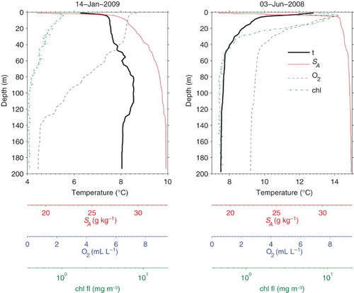
Below the near-surface, water properties are relatively uniform down to the bottom in summer, but in winter we see an intermediate water temperature maximum between depths of 70 and 130 m. However, winter dissolved oxygen concentrations decrease and salinities increase in this depth range without showing a local maximum or minimum. Water properties in winter are relatively uniform only in deep water below about 140 m.

Phytoplankton, identified through chlorophyll fluorescence, are present year-round. In winter, concentrations are generally low (around 1 mg m⁻³ at most), with a surface maximum and a gradual decrease with increasing depth that at least in 2009 extended to 80 m. In summer, values are highest below the surface at a depth of 5 to 10 m (reaching 20 mg m⁻³ or occasionally more), and the chlorophyll fluorescence signal sinks to a background noise level at a depth of about 40 m.

The timing of the seasonal cycle in surface temperature is relatively constant from year to year, with annual maxima in July or early August and minima in January or February (Fig. 4b). However, the minimum and maximum temperatures vary considerably from year to year. Summer peak temperatures decreased from more than 19°C in 2004 to less than 17°C in 2010 onwards. Winter minima vary from less than 6°C in 2008 to nearly 9°C in 2010 (Fig. 4a). Although winter minimum temperatures are the same for both Swale and Sarita stations, summer maxima are often several degrees higher at the more sheltered Sarita station.

Fig. 4 (a) Temperatures at 2 m for the Sarita and Swale stations. (b) The annual signal in near-surface temperature. Times during which deep water density (below 140 m) is increasing are shaded in grey.

Surface salinities tend to be lower in winter (Fig. 5b) and are usually highest in September at the end of the dry summer. Surface salinities in Trevor Channel at the Sarita station reached a minimum of about 10 g kg⁻¹ at 2 m in 2007 and are generally less than surface salinities in Eagle Channel. The difference is about 5 g kg⁻¹ in summer but can be as large as 15 g kg⁻¹ in winter.

Fig. 5 (a) Salinities at 2 m for the Sarita and Swale stations. (b) The annual signal in near-surface salinity. Times during which deep water density (below 140 m) is increasing are shaded in grey.

To examine seasonal cycles in deeper waters more insight can be obtained by examining a time-depth contour plot (Fig. 6). Taking the 2008–2009 period (for which data quality and coverage is best) as an example of typical conditions, near-surface water temperatures reach their maximum in August and their minimum in February (Figs 6a and 6e) for both Sarita and Swale stations. Although the upper water column is always stratified, and the amplitude of the seasonal cycle in temperature decreases rapidly from the surface through the upper few metres, these cycles are visible down to around 30 m at both locations.

Fig. 6 Seasonal cycles of (a) temperature, (b) salinity, (c) density, and (d) dissolved oxygen for Swale station in Eagle Channel. (e) to (h) As in (a) to (d) but for Sarita station in Trevor Channel. Time interval plotted is from June 2008 to August 2009. The white lines in (d) and (h) mark the hypoxic limit (1.4 mL L⁻¹).

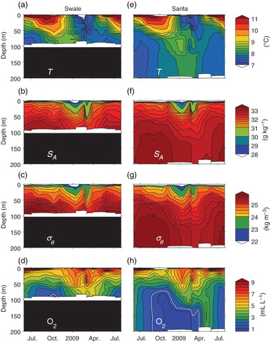
From 70 to 130 m at the Sarita station and from 70 m to the bottom at the Swale station the seasonal cycle in temperature is somewhat different than near the surface. Temperatures in this intermediate layer are at a minimum in the summer and a maximum in December (Swale) or January (Sarita). Temperature contours in this depth range are more vertical, suggesting that the water mass at any one time is relatively homogeneous. Between 30 and 70 m, temperatures are a mixture of the near-surface and intermediate temperatures.

Finally, below 140 m at the Sarita station water mass properties are almost uniform in depth at any one time although they change seasonally with a cycle that is offset from that of the near-surface and intermediate layers. These deep basin waters are coldest in summer, as for intermediate waters, but warmest in February, later than the time of the peak temperature in intermediate waters.

Near-surface salinities (Figs 6b and 6f) are at a maximum in late summer but are considerably lower during the winter when freshwater input is greatest. The timing of peak freshness shifts slightly later in intermediate waters although a boundary near 70 m separating near-surface and intermediate waters is not as obviously visible as it was for temperatures. Deep waters (below 140 m) are again identified as a region where properties are always relatively uniform in depth at any one time; peak freshness occurs in March. This deep water is not always perfectly mixed. Although densities (Figs 6c and 6g) are primarily controlled by salinity, on occasion saltier water can be observed above slightly fresher waters; in these cases a small temperature gradient is sufficient to stabilize the water column.

Dissolved oxygen levels near the surface (Figs 6d and 6h) are always high, especially in summer, but decrease down to 70 m. At intermediate depths oxygen levels are highest in January and February but lowest in October and November. Concentrations are relatively uniform with depth below about 140 m, as with temperature and salinity. However, peak oxygen levels in the deep water occur in May, some time after peak temperature and salinity, and lowest values occur in January.

Oxygen levels in the deep water are sufficiently low that hypoxia is a concern. Although hypoxia refers to a state of internal stress in animals and should probably be defined in terms of a critical oxygen partial pressure (Hofmann, Peltzer, Walz, & Brewer, 2011), here we follow widespread practice and equate “coastal hypoxia” in terms of a concentration level below 1.4 mL L⁻¹ (∼60 μmol kg⁻¹). Under these conditions coastal ecosystems are dominated by species adapted to low oxygen conditions.

Lowest levels of oxygen are slightly below the coastal hypoxic limit in significant sections of the water column at Sarita station. This hypoxic limit is as shallow as 70 m during the fall, but during the first part of 2009 the hypoxic limit occurs somewhat deeper, near depths of 130 m. Hypoxia is not present during the spring and summer. In contrast, dissolved oxygen concentrations near the bottom at Swale station just barely reach the hypoxic limit only in the October survey.

Analysis of these seasonal cycles suggests that there are three distinct layers in Eagle Channel and four in the deeper parts of Trevor Channel and Alberni Inlet. Winter surface waters (i.e., in the upper 4 m) are much fresher, and summer surface temperatures are warmer, in the more sheltered Sarita profiles. Seasonal cycles of surface temperature and salinity are related to seasonal cycles of solar insolation and freshwater inflow.

Next, in a near-surface layer down to 70 m (and especially in the upper 30 m) there is little superficial difference between the two locations, and this must be related to the relatively open connection above about 22 m, with effects spread to greater depths by vertical mixing and/or tidal processes that constantly allow water to slosh over sills. Again, water properties are related to seasonal cycles of solar insolation and freshwater inflow.

Intermediate water is found at depths of 70 to 130 m. Although there is a strong seasonal cycle in the intermediate water, the timing of seasonal maxima and minima in this layer is complex, can be different for different parameters, and can also be quite different from the timing of seasonal cycles nearer the surface. Hypoxic conditions can appear for several months in the late summer and fall.

Finally at depths below 140 m inside Trevor Channel and Alberni Inlet, there is relatively homogeneous deep water. The timing of maxima and minima for different parameters in this deep layer are again different, both from each other and from those in the intermediate and surface waters. The depth of the upper boundary is likely related to the depths in Junction Passage, again with inflowing water spread deeper by vertical mixing. Hypoxic conditions in the deep water occur for up to half the year in fall and winter.

c Near-Surface Waters: Freshwater Content

Because surface salinities can be quite variable (Fig. 5), possibly as a result of localized mixing, a more stable measure of stratification in the surface and near-surface waters is the freshwater equivalent (FWE), which represents the depth of fresh water with a salinity of zero that would be mixed with saline water from a depth of H = 70 m (i.e., “ocean” inflow water in a standard estuarine circulation with surface outflow and deeper inflows) to produce the measured salinity profile over the upper 70 m. This is calculated by solving a salt conservation equation for the water column:(2) The FWE ranges from a minimum of 1 m in the summers of 2009 and 2013 to more than 4 m during some winters (Fig. 7a). The FWE is generally highest in winter and lowest towards the end of summer. The Sarita FWE tends to be slightly larger than the Swale FWE, perhaps because the fresh water from Alberni Inlet can spread horizontally over a larger area in Eagle Channel or because fresh water tends to exit to the coast via Trevor Channel.

Fig. 7 (a) FWE and (b) depth-integrated chlorophyll biomass. The mean summer conditions (between the spring increase and the fall decrease in chlorophyll biomass) are shown as horizontal bars. Times during which deep water density is increasing are shaded in grey.

A crude estimate of the time scale for changes in oceanographic structure related to changes in river flow is the freshwater residence time of the area between the Somass river and the time series stations. This is found to be less than a week in winter by dividing a typical total freshwater volume by a mean freshwater inflow rate of approximately 400 m³ s⁻¹ (double the winter Somass River flow). In summer, when the freshwater inflow is dominated by the Somass River and most of the other rivers have very low flows, the freshwater inflow rate is only about 100 m³ s⁻¹. Even though the FWE is also smaller (around 2 m), the residence time for surface waters increases to around two weeks.

These estimates are probably higher than the true freshwater residence times. Because it is unlikely that the interface between estuarine inflow and outflow is as deep as 70 m, so some of the FWE calculated using Eq. (2) probably enters Barkley Sound at depth as part of the estuarine circulation. Taking a shallower reference level to avoid this would reduce the calculated FWE and, hence, any calculated residence time. For example, taking H = 30 m in Eq. (2) results in residence time estimates of less than a week in both winter and summer.

In any case, the residence time of surface waters is quite short relative to the monthly survey spacing. The relatively short residence time implies that surface stratification can change rapidly in response to specific rainfall events. Winter levels of FWE when rainfall events are common are, therefore, often large but quite variable.

During summer, FWE levels are less variable partly because residence times are longer but also because there are fewer rainfall events. Mean values at Sarita can vary from 1.3 m in 2009 to 3.7 m in 2007. This would suggest that summer freshwater inflows were largest in 2007 and smallest in 2009; the Sproat River flow measurements confirm this.

d Near-Surface Waters: Primary Production

Chlorophyll concentrations are also highly variable. Depth profiles of chlorophyll fluorescence show that most of the biomass occurs shallower than 20 m although a fluorescence signal above the noise level can sometimes be measured to much greater depths (e.g., Fig. 3). To avoid dealing with the complexities of changing depth distributions of chlorophyll, a depth-integrated biomass is considered here, estimated by vertically integrating the fluorescence signal once the “background” signal at depth, taken to be an instrument artifact, has been subtracted.

There is a seasonal pattern of phytoplankton biomass, high in summer and relatively low (although not zero) in winter (Fig. 7b). Biomass time series at the two stations are reasonably correlated suggesting that temporal variability has a wide spatial scale although, in general, values are somewhat higher in Eagle Channel than in Trevor Channel. In addition, there are large interannual differences in the summer levels that are superimposed on the short-term variability.

Although the monthly sampling is too coarse to fully resolve typical phytoplankton blooms, in none of the five years for which chlorophyll measurements are available has there been any sign of a typical temperate-region “large spring bloom” whose biomass dominates the annual mean, as seen in, for example, the nearby Strait of Georgia (Harrison, Fulton, Taylor, & Parsons, 1983). Instead biomass levels increase sometime during the February to May period, reaching a roughly constant level that characterizes the rest of the summer. The mean summer (May–September) biomass was almost 200 mg chl m⁻² in 2009 but only 70 mg chl m⁻² in 2007. Winter levels are of the order of 20 mg chl m⁻². The timing of the spring increase is quite variable. Biomass reached summer levels in March of 2006, 2008, and 2010, April of 2007, and February of 2009.

Although only five years of chlorophyll data are available, quite strong correlations exist between the mean summer biomass and several other features. First, larger mean summer biomasses are almost perfectly correlated with lower summer mean FWE (Fig. 8b). Large summer biomass also correlates with an earlier timing of the spring increase (Fig. 8c). Earlier spring increases are associated with smaller summer FWE (Fig. 8a) although the precise relationship is different at the Swale and Sarita stations.

Fig. 8 Correlations between (a) time of the spring increase and summer FWE; (b) mean summer biomass and mean summer FWE; (c) mean summer biomass and the timing of the spring increase.

e Deep Water Renewal

Spatial and temporal variability below 70 m is related to renewal processes. In order to characterize these processes, time series of densities at different depths are examined (Fig. 9a). Measurements at 80 m at Swale are taken as representative of near bottom values in Eagle Channel (80 m is chosen as a “bottom value,” even though it is almost 20 m above the bottom at Swale because a measurement at that depth is available for all surveys). These values closely match bottom water densities measured at the Folger node when these are available from 2009 onwards. Measurements at 80 m in Trevor Channel at Sarita represent the intermediate water there. Finally, densities at 170 m are representative of the relatively homogeneous deep or bottom waters (below 140 m) in Trevor Channel and Alberni Inlet.

Fig. 9 (a) Density of the deep and intermediate waters. (b) Alongshore winds at La Perouse and sea level at Bamfield (low-pass filtered with a two-week cutoff). Times during which deep water density is increasing are shaded in grey.

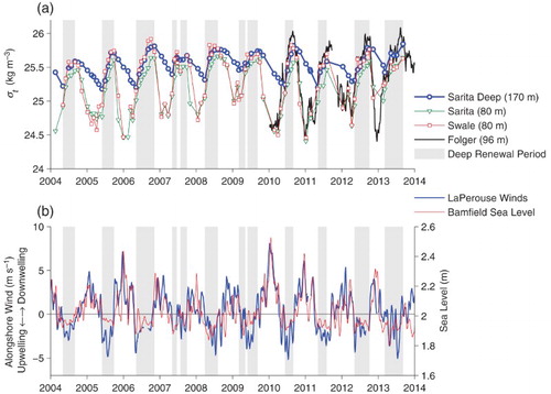
During winter, densities at 80 m at Swale and Sarita are almost identical (Fig. 9a). However, during summer, Swale densities at 80 m are slightly greater than Sarita densities at 80 m and are also often greater than Sarita densities at 170 m. During summer, dense bottom water from Eagle Channel must flow through Junction Passage and down into the bottom of Trevor Channel and Alberni Inlet as a density current, renewing the deep water. Densities at 170 m rise in response to this renewal. Renewal periods can, therefore, be precisely quantified by defining them as periods during which bottom water densities at Sarita increase. These periods are shaded in grey in Figs 4, 5, 7, 9, and 10.

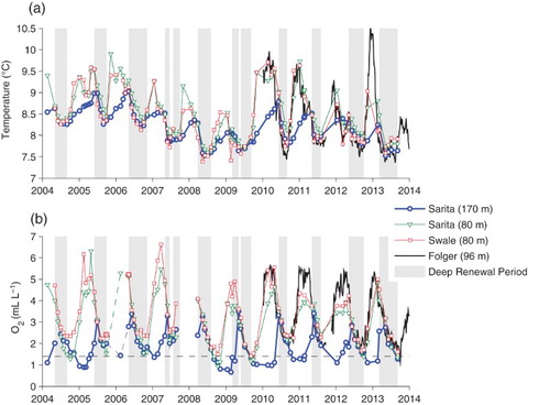
Fig. 10 (a) Temperatures and (b) dissolved oxygen concentrations in the deep and intermediate waters. Times during which deep water density is increasing are shaded in grey.

Conversely, during the rest of the year there is no (or at least only very little) advective inflow into the deep water region. Intermediate water at 80 m is much lighter than deep water, which is then stagnant. However, the density of this deep water drops slowly and steadily through the winter. This must be a result of vertical eddy-diffusive processes bringing fresher intermediate waters down into the deep layer.

The alternating dominance of advection and vertical diffusion leads to an annual “sawtooth” shape for the 170 m deep water time series. Density maxima occur near the end of the summer after a rapid rise in density caused by advection, and density minima occur in spring after a longer more gradual drop caused by vertical diffusion.

The period during which deep renewal occurs (i.e., during which deep water densities increase) varies from year to year (Fig. 9a). The longest periods (6 months) occurred in 2006 and 2013, and the shortest (just under 3 months) occurred in 2010. The renewal is not necessarily continuous over the summer. Densities drop for short periods during the summers of 2007 and 2009, at approximately the same rate seen in winter, suggesting interruptions in the renewal. Interruptions may also occur on even shorter time scales not resolved by our measurements. Thus, in July 2009 the Swale deep density is briefly less than the Sarita deep density even though the Sarita deep density is monotonically increasing in our observations.

The density increase over the summer also varies from year to year. However, the overall length of the renewal period does not correlate with the size of the overall density increase. The largest changes in density in summer occured in both 2006, which had the longest renewal period, and 2010, which had the shortest. The time at which renewal begins also varies from year to year. Although in most years renewal begins in early May, it began in March in 2008, 2009, and 2013 but only in June in 2010.

The inflow of dense water into Eagle Channel, where it can act as source water for the renewal of the deep water in Trevor Channel and Alberni Inlet, is a result of coastal upwelling processes that bring this dense water from the deep Pacific Ocean up onto and across the shelf. The strength of these processes can be quantified by considering winds in the along-shore direction measured at the nearby offshore weather buoy C46204 (La Perouse, Fig. 1).

The proposition that along-shore winds at La Perouse (Fig. 9b) provide an effective measure of upwelling can be verified by first considering their relationship with coastal sea levels. Coastal upwelling theory (e.g., Thomson, 1981, ch. 5) suggests that if along-shore winds drive a perpendicular cross-shore flow near the surface due to Coriolis effects, these winds should also be highly correlated with subtidal sea levels at the coast. Sea levels are measured at Bamfield, and the sub-tidal variations do covary with the along-shore winds (Fig. 9b) with the expected relationship. Upwelling-favourable winds in summer associated with offshore surface transport cause coastal sea levels to drop by about 10 cm. Conversely, downwelling favourable winter winds associated with onshore transport can cause the sea level at the coast to rise by anywhere from 5 to 40 cm.

Upwelling theory further suggests that offshore flow near the surface is compensated for by an onshore flow in underlying waters, and this onshore flow is composed of more dense water that may originate from deeper layers of the ocean below the shelf break. In fact, periods of upwelling-favourable winds coincide almost exactly with deep renewal periods, as indicated by the grey-shaded periods during which densities increase in the deep waters of Trevor Channel and Alberni Inlet (Figs 9a and 9b). This match even includes the short mid-summer breaks in 2007 and 2009. Not only does this match indicate that coastal upwelling governs renewal, but the lack of delay in the response also suggests that transport of dense water into Eagle Channel is relatively rapid (occurring within a period month) in response to the winds.

During the renewal period, the deep basin densities in Trevor Channel and Alberni Inlet increase, but this increase slightly lags the increasing densities on the sill in Eagle Channel. A lag will arise from the finite residence time of the deep basin. The deep basin (below 140 m) is relatively uniform in its properties at all times, both vertically and horizontally, compared with the range of seasonal variations (see Fig. 6 and Section 4.g) but these properties change substantially over time. That is, the basin is close to being fully mixed. A fully mixed conservative tracer in a deep basin of fixed volume will be modified by an inflow of some external water with characteristics and a compensating outflow of basin water with characteristics up into the intermediate layer, according to:(3) Salt content is conservative. Strictly speaking, temperature and density are not conservative, but the errors that arise from treating them this way are negligible in the rough calculations discussed here.

During the renewal period, the characteristics of the source water (as observed at a depth of 80 m near Swale) change with time. If the source water characteristics change linearly with a slope (i.e., ), and the basin waters also increase with the same slope but a slight time lag , , with a constant inflow rate , then Eq. (3) can be solved to show that the basin residence time , defined as the basin volume divided by the boundary inflow (or outflow), is directly related to this lag time: . The basin residence time is an “e-folding” time for the system, during which 63% of the volume would be exchanged after a step-change in input.

The lag time of the rise during renewals is less than the monthly sampling interval (Fig. 9a). This suggests a deep water residence time, during renewals, of a few weeks at most. Because the renewal period is three to six months long, the length of the renewal time is much greater than the residence time. The conclusion is that deep waters are comprehensively flushed and renewed many times during the summer. In addition, the close tracking between Sarita deep-water characteristics and those at the bottom at Swale and Folger in summer also implies that the deep water in Trevor Channel and Alberni Inlet provides a good record of the characteristics of shelf bottom water during the summer upwelling period.

During winter, when the deep water is apparently stagnant, it is affected only by vertical eddy-diffusive processes. The behaviour of a conservative deep water tracer in response to a vertical exchange with intermediate water of characteristics can be modelled as(4) Using Eq. (4) and the tracer observations in Fig. 9a, we can estimate the residence time during stagnant periods to be days. Thus, even during these “stagnant” periods (which last six to nine months) the deep water undergoes significant renewal. However, the deep water conditions at this time are not easily related to conditions on the shelf.

The effects of renewal processes can also been seen in seasonal cycles of deep temperature and dissolved oxygen (Fig. 10). During renewal periods, the temperatures of inflowing waters are initially warm but cool rapidly over the following months. Then, near the end of the renewal period, this trend reverses and inflowing waters have slightly warmer temperatures (Fig. 10a). Once deep renewal processes end, temperatures continue to rise at a reasonably steady rate through the winter in the deep basin but increase quite rapidly until reaching a winter plateau in intermediate waters. Although no advective renewal is occurring, warmer waters from above are diffusing down into the deep basin in winter.

The deep inflows at the start of renewal periods are also relatively high in dissolved oxygen (3–4 mL L⁻¹), producing the seasonal maximum in deep basin oxygen concentrations. However, oxygen levels quickly drop in the inflowing water and towards the end of the renewal period these waters contain less than 2 mL L⁻¹ of oxygen (Fig. 10b). Thus, in general, oxygen levels rise only at the beginning of the renewal period then slowly decrease during renewal.

During winter, oxygen levels in the deep water of Trevor Channel and Alberni Inlet also exhibit a different pattern than temperature and density (and salinity). Rather than rising in response to diffusion from above, they often continue to decrease until the end of the calendar year, after which they increase slightly in advance of the next renewal.

Dissolved oxygen levels in the winter deep water will increase because of diffusion from above but may also decrease because of biological respiration. Equation (4) can be modified to include both effects by the addition of a term involving a system oxygen utilization rate (OUR) :(5) In a fully mixed volume near the bottom would represent the combined effects of pelagic and benthic oxygen utilization. Substituting estimates of already found using Eq. (4) into Eq. (5) and using the observations in Fig. 9b, the deep basin OUR in winter is calculated to be  mL L⁻¹ yr⁻¹ (0.3 mmol O₂ m⁻³ d⁻¹). Integrated over the volume of deep water and divided by the area of the deep basin, this is equivalent to an areal utilization rate of about 15 mmol O₂ m⁻² d⁻¹. The latter would be a more appropriate value for comparison if benthic respiration dominated, whereas the former would be more appropriate if pelagic respiration dominated.

A constant oxygen utilization rate and vertical diffusive transport is not inconsistent with the initial drop and later rise in oxygen levels in the fall, winter, and spring. Oxygen levels can decrease in the period soon after renewals end because the oxygen utilization rate is larger than the rate at which diffusion brings new oxygen down. At this time oxygen levels in the intermediate water are still rising so that the vertical gradient is relatively small. However, in the spring the vertical oxygen gradient is large, and diffusion effects may be larger than oxygen utilization. Thus, deep oxygen levels can rise slightly.

Although all deep water variables are characterized by a strong seasonal cycle (albeit with variations in the timing of maxima and minima) the year-to-year variability between them is uncorrelated. Bottom water densities were greatest in 2014 and almost equally dense in 2010 and 2006 (Fig. 9a). The annual density maximum was lightest in 2004. However, annual minimum temperatures drop monotonically from a high of 8.26°C in 2004 and 2005 to 7.53°C in 2008, rising thereafter (Fig. 10a). Annual maximum temperatures are highest in winter 2005/2006, and lowest in winter 2008/2009. They may even have briefly exceeded 10°C in winter 2012/2013 following temperatures at Folger, but the interval between CTD surveys was too large to capture this.

On the other hand, dissolved oxygen levels show no obvious trends (Fig. 10b). Minima and maxima do change slightly from year to year. Winter minima are apparently highest in 2006 or 2007 and lowest in early 2009. However, the differences are on the order of the estimated accuracy of the measurements. Thus, it is not possible to say whether hypoxic conditions are becoming more severe. Winter levels in the deep basin are always slightly under the hypoxic limit of 1.4 mL L⁻¹ (with annual minima in this time series between 0.6 and 1.4 mL L⁻¹), but winter levels near the bottom of Eagle Channel were hypoxic only briefly in the fall of 2008.

Interestingly, there does not seem to be any relationship between deep renewal processes and near-surface characteristics. The FWE does tend to decrease rapidly around the onset of deep renewal (Fig. 7a). However, the change in offshore wind direction also coincides with a dramatic change in the weather and the amount of river flow (not shown), so this correlation does not necessarily imply a causal relationship. Phytoplankton biomass (or equivalently the timing of the spring increase) is also unrelated to the timing of the beginning of the deep renewal period, which is at the transition from downwelling to upwelling winds (Fig. 7b). In 2007 and 2008 the two coincide, but the spring increase is one month earlier in 2009 and two months earlier in 2006 and 2010.

f Intermediate Water Renewal

During fall, winter, and spring, when the deep water in Trevor Channel and Alberni Inlet is not undergoing summer renewal, the intermediate water just above has temperature and salinity characteristics quite similar to those near the bottom in Eagle Channel, at Swale and (when available) at Folger. At those times downwelling-favourable winds result in decreased bottom densities on the shelf and, hence, in Eagle Channel (Fig. 9). Strongest downwellings (e.g., in the winters of 2005/2006, 2009/2010, and 2010/2011) correlate with the least dense bottom waters at Swale in Eagle Channel.

These bottom waters in Eagle Channel then enter Trevor Channel–Alberni Inlet at intermediate levels, underneath the light near-surface layer transporting fresh river water seaward. Because these intermediate depths are not isolated behind a sill, horizontal density differences between the mouth and interior of Barkley Sound (i.e., between Folger, Swale, and Sarita), at the same depth, are small (Fig. 9a). This is true even as the density itself undergoes a rapid decrease in the fall and winter, followed by an increase in the spring as the strong winter downwelling relaxes and reverses into upwelling.

Patterns of temperature in intermediate waters at Folger, Swale, and Sarita during downwelling periods also change rapidly and synchronously (Fig. 10a). Not only do intermediate temperatures increase rapidly at the end of the deep renewal period, but even small temporary decreases in temperature (e.g., in early 2005 and 2006) are almost instantaneously seen in both the Swale and Sarita time series. Temperatures at Sarita tend to lag those observed at Swale by only a few weeks at most. This is most obvious in late 2004 and 2008. At other times the lag is less obvious because rapidly varying changes are undersampled in our monthly time series. These rapid and synchronous changes imply that the residence time of the intermediate water in Barkley Sound must also be short, no more than a few weeks. Intermediate water temperature and salinity in the Sound reflects shelf conditions.

However, in spite of this short residence time, the levels of dissolved oxygen in the intermediate water sometimes vary significantly among Folger, Swale, and Sarita in winter (Fig. 10b). Bottom concentrations of oxygen at Folger from January to the onset of upwelling are around 5 mL L⁻¹ in 2010–2013, sometimes similar to Swale values and sometimes around 1 mL L⁻¹ higher, and presumably this is also true in earlier years. The interannual variability makes it difficult to generalize with certainty, but a drop of about 1 mL L⁻¹ in two weeks is equivalent to 3 mmol O₂ m⁻³ d⁻¹, about 10 times larger than the OUR inferred for the deep water in Trevor Channel and Alberni Inlet.

g Spatial Variability in Intermediate and Deep Waters

Although the CTD time series provides insight into differences between Eagle Channel, which is relatively shallow, wide, and open to the coastal ocean, and the deeper, more sheltered Trevor Channel, this deep channel, which extends for another 38 km through Alberni Inlet, is not completely spatially uniform in its properties. These spatial variations can be seen in two longitudinal sections (Fig. 11), which were occupied in June 2007 (early summer) and February 2009 (winter).

Fig. 11 Sections along Trevor Channel and Alberni Inlet in June 2007 and February 2009. (a) Summer temperature, (b) winter temperature, (c) summer salinity, (d) winter salinity, (e) summer dissolved oxygen, and (f) winter dissolved oxygen. The white line marks the hypoxic limit in winter. Distances are inshore of the coast. The Sarita station is at kilometre 27.

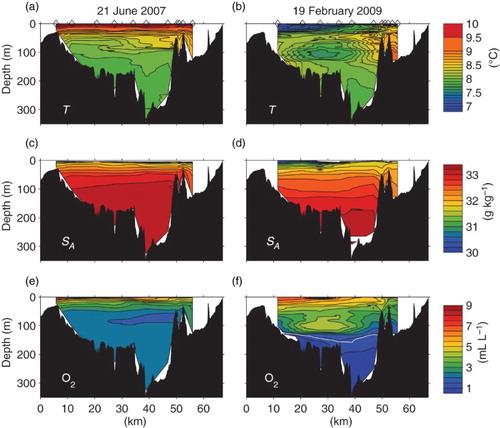
In summer the waters below about 70 m are relatively similar in salinity throughout the main basin (kilometre 5 to 49) although at depths between 50 and 100 m a slight increase in salinity towards the first sill near Sproat Narrows at kilometre 49 (Fig. 11c) is density-compensated by slightly warmer temperatures (Fig. 11a). Summer temperatures in this depth range are decreasing in time at Sarita (Fig. 6e) so this spatial change simply reflects the speed at which waters farther up the inlet are being replaced by inflows. Summer oxygen levels are greater than 2 mL L⁻¹ in the main basin and relatively constant, with the exception of a slight decrease, also at depths of 50 to 100 m, near the head (Fig. 11e).

Although we do not have many measurements within the inner basins inshore of kilometre 55, waters within these inner basins are warmer and fresher than waters seaward of the sill in summer. The inner basins are also more oxygenated than the outer basin at the same depths.

In the winter section waters below 70 m are considerably more stratified, with a visible salinity gradient down to the bottom (Fig. 11d). In contrast, dissolved oxygen values are sharply layered. Below about 140 m waters are hypoxic and relatively uniform over the entire area. However, above this level, a cold and highly oxygenated intermediate water is seen centred at Junction Passage (kilometre 27). This inflowing water mass is bounded to both the south and north of Junction Passage by a region of complex vertical profiles which show interleaving between the inflowing and existing water masses.

5 Discussion

a Circulation and Hypoxia

The observations described above provide a good description of the seasonal and interannual changes in Barkley Sound, and the different residence time calculations based on these observations can be combined into a coherent picture of the overall circulation and its response to different forcing factors. This is best approached by vertically dividing the water column into several different regions.

First, surface waters, especially in the well-stratified upper few metres but generally down to about 70 m are largely controlled by freshwater runoff and solar insolation, and the degree of freshness is in equilibrium with runoff at time scales greater than the freshwater residence time, which is around one to two weeks at most. In the winter, these waters are cold and fresh, whereas in summer they are warm and saline. Surface waters are warmest in August but most saline in September just before fall rains lead to increases in riverflows.

Surface waters flow seawards and subsurface waters landwards in an estuarine circulation. With a freshwater residence time of about one week, mean surface currents over the approximately 60 km between the Somass River and the ocean must be around 10 cm s⁻¹. This is not inconsistent with limited measurements at Sproat Narrows reported by Farmer and Osborn (1976) although they also found a high degree of short-term variability associated with winds.

Second, intermediate waters from 70 m down to 130 m are closely linked to shelf waters from the open coast, and conservative properties like temperature and salinity within Trevor Channel lag those from the coast by less than a month. This is true year-round. In fall, winter, and spring the changes in the intermediate water of Trevor Channel and Alberni Inlet are directly linked to changes in Eagle Channel with a delay of one or two weeks. Inflowing waters can be seen as intrusions radiating from Junction Passage but outflows are less obvious. Currents in Junction Passage are strongly tidal and are also variable at scales of a few days in response to short-term changes from upwelling to downwelling-favourable winds offshore (Stucchi, 1983). Although these short-term changes are filtered out in Fig. 9b, they suggest that exchange between the two channels is probably driven by time-variable horizontal eddy- and tidal-pumping processes, rather than a steady mean flow.

During the deep renewal period in summer, the Eagle Channel waters sink to the bottom in Trevor Channel and Alberni Inlet and rapidly flush out the deep water, which is then uplifted into intermediate depths. The lag in measured water properties between the shelf and intermediate waters is greater than in winter but still less than one month. Intermediate temperatures are generally warmer, salinities lower, and oxygen levels higher during downwelling, and waters are colder, saltier, and lower in oxygen during upwelling. In many years oxygen levels in intermediate waters can briefly drop below a hypoxic limit in fall, at or just after the end of the deep renewal period, but this hypoxia is not seen after October.

Third, deep basin waters below 140 m are also linked to the open coast, but this linkage is modulated by renewal processes. The renewal period is set by upwelling-favourable winds occurring offshore. It begins sometime between March and June and lasts from three to six months but is occasionally interrupted when winds reverse for short periods. During renewal periods deep basin characteristics lag open coast values by only a few weeks. This in turn implies that the residence time of water in the deep basin during renewals is only a few weeks at most, so the deep water is replaced many times over the summer. The replacement inflow comes through Junction Passage, which is only about 1 km wide. Assuming that the inflow is in a layer about 20 m thick (i.e., near the bottom), this implies steady inflow velocities of only about 4 cm s⁻¹, entirely consistent with current meter records in that area (Stucchi, 1983).

During renewal, deep water density increases (by definition) and temperatures initially decrease and then increase. Oxygen levels, which are highest at the start of the renewals, decrease to near-hypoxic levels. Renewal timing and the length of the renewal period can vary greatly from year to year but these factors do not seem to be related to the magnitude of the density increase that occurs during renewal. It is possible that time-integrating winds to produce a cumulative upwelling index (as in, e.g., Connolly et al., 2010) may have some predictive capability for this increase but initial tests were inconclusive.

During the rest of the year, although “stagnant” and not directly affected by advective processes (hence, independent of shelf conditions), deep waters are modified by vertical eddy-diffusive processes that replace a substantial fraction of deep water volume before the next deep renewal period. Density and salinity decrease and temperature increases. Oxygen levels decrease initially becoming hypoxic in most years. This tends to occur early in the stagnation period. However, oxygen levels often increase towards the end of the stagnation period, reaching a maximum at the beginning of the renewal period. Part of this increase is caused by vertical diffusion rates varying with time in response to changes in the vertical gradient in oxygen, so the balance with oxygen utilization can also vary with time.

The general “sawtooth” pattern for density, temperature, and oxygen is not unusual for northeast Pacific fjords (even as far north as 53°N; Wan, Hannah, Foreman, & Dosso, 2017), but previous investigations have generally been limited to those surrounding the Salish Sea on the east side of Vancouver Island. The renewal period for such fjords tends to be in late fall or winter, not in summer (Pickard, 1975). However, these Salish Sea fjords are not renewed directly from the Pacific but rather from intermediate or near-surface waters of the Strait of Georgia, whose deep waters are renewed in summer (Pawlowicz, Riche, & Halverson, 2007). Renewals of Nitinat Lake, a fjord-lake southeast of Barkley Sound, are also different (depending on surface water conditions) because the sill depth is only about 2 to 5 m deep there (Pawlowicz, Baldwin et al., 2007).

Thus, although the topography of Barkley Sound is complex, with numerous islands, channels, and subsidiary inlets, the bulk characteristics of its circulation dynamics can be described relatively simply. There is a standard estuarine circulation with surface outflow and deeper inflow in surface and near-surface waters, responding to local conditions, a continuous circulation in intermediate waters, and a renewal cycle in deep waters controlled by offshore conditions. Because the local and offshore forcing factors do not change synchronously, the surface and deep circulation patterns are somewhat independent. Note that the near-surface estuarine circulation presumably extends all the way to the head of Alberni Inlet. However, the sills at Stamp and Sproat Narrows would change the timing and character of deep renewals in the inner basins, relative to those for the main basin of the Inlet. For comparison, renewals have recently been studied for the inner basin of Effingham Inlet which is also joined to Barkley Sound, and these renewals are both intermittent (averaging about two years apart in recent decades) and not as closely linked to wind conditions as those of the Barkley Sound main basin (Thomson et al., 2017).

This analysis, therefore, suggests that Barkley Sound measurements in intermediate and deep waters could be a useful proxy for monitoring conservative physical parameters on the shelf, at least at depths of around 100 m. However, this monitoring capability is not necessarily true for nonconservative tracers such as oxygen because biogeochemical processes within the Sound, controlled by local factors, can sometimes significantly affect nonconservative tracers even during these relatively short residence times, so that these may be different than shelf values. Also, note that the shelf here is quite complex, and depths on the shelf can exceed 150 m in some holes and canyons. Barkley Sound measurements may not be informative about conditions at those depths on the shelf.

b Oxygen Utilization Rates

The local utilization of oxygen is presumably at least partly driven by the decomposition of sinking phytoplankton biomass but may also result from the decomposition of terrestrially derived organic material within these restricted waters. However, during the deep renewal period a utilization rate of 0.3 mmol O₂ m⁻³ d⁻¹ would change oxygen levels by only 0.1 mL L⁻¹ over two weeks. This is smaller than our measurement accuracy. Thus, as long as this fall-winter-spring mean utilization rate is not too different during the summer renewal period, the apparent drop in deep oxygen levels will be almost entirely related to the presence of low oxygen water on the shelf, which is advected into Barkley Sound, and not to oxygen utilization within the Sound.

The estimated oxygen utilization rate of 0.3 mmol O₂ m⁻³ d⁻¹ within Barkley Sound is slightly, but not significantly, larger than values found in nearby fjord-type estuaries (note that this value may also change from year to year, but such variations are within the uncertainty of our data). A combined rate of approximately 0.2 mmol O₂ m⁻³ d⁻¹ was estimated as an annual rate for the deep Strait of Georgia by Pawlowicz, Riche et al. (2007). Although the biological processes must differ, note that a nearby anoxic fjord (Nitinat Lake) has an estimated residence time of only about five years (Pawlowicz, Baldwin et al., 2007) and is renewed by oxygenated surface waters. This would suggest that oxygen is used there at an annual rate of approximately 0.2 mmol O₂ m⁻³ d⁻¹.

Alternatively, Bianucci et al. (2011), using a two-dimensional “slice” biogeochemical numerical model of this shelf area, found that sediment uptake of oxygen was far more important than water column respiration. Their benthic uptake rate on the shelf, about 14 mmol O₂ m⁻² d⁻¹ derived from model output, is very similar to the value of 15 mmol O₂ m⁻² d⁻¹ we estimate in the deep basin of Barkley Sound under the assumption that all oxygen utilization occurs at the bottom. Similar values were also found in the more recent three-dimensional model described by Siedlecki et al. (2015), which compared well with direct measurements of sediment oxygen consumption on the Washington Shelf (Hartnett & Devol, 2003).

Thus, it seems likely that our estimated OURs are reasonable for this region. However, a rate of 0.3 mmol O₂ m⁻³ d⁻¹ is quite low compared with estuaries in general. Pelagic respiration rates for 22 different estuaries were summarized by Hopkinson, Jr. and Smith (2005), finding values from 1.7–88.4 mmol O₂ m⁻³ d⁻¹. Alternatively, Hopkinson, Jr. and Smith (2005) describe areal system respiration rates ranging from 69–631 mmol O₂ m⁻³ d⁻¹, with a mean of 294 mmol O₂ m⁻² d⁻¹. These values are also somewhat larger than our 15 mmol O₂ m⁻² d⁻¹. This is still true even if summer utilization rates are ten times higher than in winter, as is (approximately) the phytoplankton biomass.

c Controls on Primary Production

We can exploit the difference in the timing of changes in surface and deep circulations to discuss controls on primary production in Barkley Sound because a spring increase in phytoplankton concentrations occurs sometime between February and April (one to three months before the deep renewal begins), and years in which this increase occurs earlier are also years when surface waters are both more saline (less FWE, likely in response to less freshwater inflow) and have greater phytoplankton biomass during the rest of the spring and summer. Also, after the spring increase, biomass levels remain similar all summer and, in particular, are similar before and after the onset of upwelling and deep renewal (most visible in 2006 and 2010, see Fig. 7b).

Coastal upwelling acts to bring deep nutrients to the surface on continental shelves where they can support primary production. The lack of any observed change in biomass within Barkley Sound related to upwelling suggests that external nutrient supply is likely not a control on primary production here. Instead primary production is more likely controlled by processes within the Sound.

It is possible that this local control is related to grazing, but note that biomass also undergoes a large degree of interannual variability (e.g., biomass in 2009 was about three times greater than in 2007), with dry summers (smaller river inflows and lower FWE) and earlier spring increases associated with larger summer phytoplankton biomass (Fig. 8). Spatial variability is also present, with chlorophyll levels in Eagle Channel generally higher than in Trevor Channel. This spatial pattern was also found by Taylor and Haigh (1996) who, in addition, noted that biomass was even greater in Loudon Channel.

The link with FWE, which could plausibly be linked to changes in the magnitude of surface outflow and the generally increasing levels farther from the Somass River, suggest that biomass levels may simply depend on residence time in surface waters, with growth occuring until the near-surface water leaves Barkley Sound. Another possibility is that earlier spring increases are associated with increased day-light in summer. The available data are not sufficient to test this hypothesis. However, all indications are that production in the Sound is not linked to coastal upwelling but is instead related to some local forcing factor.

Finally, even though it seems likely that controls on productivity are primarily local, this does not mean that the shelf waters have no influence at all on production in Barkley Sound. For example, the depth of the fluorescence signal in winter can be as much as 80 m (Fig. 3), much deeper than the “1%” light level typically taken to be the approximate limit of the euphotic zone, which in winter is more typically between 10 and 20 m. This is likely because downwelling and/or deeper winter mixing on the shelf mixes plankton to greater depths, which then enter the Sound as part of the estuarine inflow.

d Source Waters and Interannual Variability

Where does the low-oxygen shelf water come from in summer? Deeper waters off the shelf are low in oxygen, and these are likely to be the source. A climatological relationship between oxygen and density for offshore waters, compiled from 50 years of data, is relatively tight (Fig. 12b). In the initial stages of renewal the oxygen characteristics of inflowing bottom water match those of offshore waters at the same density. Also, the temperature–salinity characteristics of this initial renewal water match those in climatological relationships offshore (Fig. 12a). However, later in the renewal period when inflows are more dense, the oxygen content of offshore waters with the same density as measured at the bottom of Eagle Channel is somewhat higher than our observations show. Alternatively, offshore waters with oxygen levels similar to Eagle Channel measurements are significantly more dense. In addition, renewal water temperatures sometimes rise during the later stage of renewal, even as density continues to rise, and this is not seen in climatological relationships offshore.

Fig. 12 (a) Correlations between climatological temperature and salinity for offshore waters. Each curve is the climatological mean for a particular month; summer and winter curves are shown differently. Also shown are curves, one per year for the deep renewal period only, showing the T/S characteristics of inflowing water at Swale and Folger stations. (b) Correlations between climatological oxygen and density for offshore waters. Although the depth of isopycnals changes dramatically over the year, the concentrations of oxygen at a particular isopycnal are relatively constant. Also shown are curves, one per year for the deep renewal periods only, showing the oxygen/density characteristics of inflowing water at Swale and Folger stations. Bottom waters at the beginning of the renewal period are lightest, and those at the end are most dense.

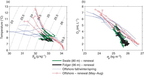
There are several possibilities. The first is that oxygen levels in the upwelled water decrease because of respiration on the shelf, and this respiration is greater in late summer. This could occur either if respiration rates are higher later in the summer or if rates remain the same and transit time across the shelf increases. A second possibility is that the shelf water represents a mixture of two waters: a deep, cold, low-oxygen water from offshore and a plausibly fresh, warm, and oxygenated water that exits Juan de Fuca Strait in late summer and then turns northward in the Vancouver Island Coastal Current (VICC). Both changes in respiration and effects of the VICC have been found to be important in a modelling study of the shelf (Bianucci et al., 2011). Note that the path by which upwelled oxygen moves from the deep ocean inshore is complicated because of the complex bathymetry and circulation patterns in this shelf region (Crawford & Peña, 2013; Siedlecki et al., 2015).

During downwelling periods there is another puzzling aspect of our oxygen measurements. By January, the bottom oxygen measurements at the Folger node show levels of approximately 5 mL L⁻¹. These levels are consistent with levels expected for offshore waters of the same density (Fig. 12b). This water presumably moves into Barkley Sound in the intermediate water layer, but if so, oxygen levels would appear to drop significantly during the transit from Folger to Sarita. A change of 1 mL L⁻¹ in two weeks is equivalent to a system oxygen utilization on the order of 25 mL L⁻¹ yr⁻¹ in the intermediate waters of Eagle Channel, which is about an order of magnitude larger than that calculated for the deep basin waters of Trevor Channel–Alberni Inlet at the same time. It seems unlikely that this could be true. It is possible that the Folger node, situated in an area of complex bathymetry within 1 km of a number of rocky offshore pinnacles whose peaks are less than 20 m below the surface, may not be entirely representative of inflowing offshore waters under downwelling conditions. However, the correlation between oxygen and density for these well-oxygenated Folger measurements is consistent with a linear extrapolation of correlations for the measurements during renewal periods, suggesting no extraordinary oxygenation. Another possibility (suggested by a reviewer) is that low-oxygen water from the deep basin is mixing upwards, reducing oxygen levels in the intermediate water.

Finally, at interannual scales, examination of the variability in each parameter that has been discussed here suggests that the variability in different parameters is uncoupled from each other. If we consider time series of annual minima (and maxima), we see that such time series would reach peaks and troughs in different years. This would also imply that the interannual variability in different parameters in shelf waters are also somewhat uncoupled. Uncoupling could result if temperature and salinity (at least) varied with time on constant density surfaces offshore. A monthly climatology (Fig. 12a) suggests that there are at least seasonal variations in offshore temperature and salinity characteristics on isopycnals and interactions between these cycles and variations in the timing of renewal may, therefore, be important. In addition, changes on decadal scales in temperature and salinity characteristics on isopycnal surfaces are also known to occur elsewhere in the California Current system (Meinvielle & Johnson, 2013), as have changes in oxygen levels on isopycnals in waters offshore of WCVI (Crawford & Peña, 2013). However, shelf processes and the influence of Salish Sea outflow in the VICC on the shelf (Masson & Cummins, 1999) may also have interannual variations. Continued measurements both inshore (e.g., in or near Barkley Sound) and seaward of the shelf break in oceanic source waters would be useful in separating these different processes.

Acknowledgements

My thanks to Ron Tanasichuk (Pacific Biological Station), who carried out many of the CTD profiles during his sampling program as well as to John Richards and Janice Pierce (Bamfield Marine Sciences Center) for operating the M/V Alta and ensuring our data were of the highest quality. Different classes and co-instructors of UBC course EOSC 473/573 over the years have provided intellectual motivation. Folger node CTD data were provided by Ocean Networks Canada. Archival data from the Institute of Ocean Sciences were provided by Peter Chandler.

Disclosure statement

No potential conflict of interest was reported by the author.

ORCID

R. Pawlowicz http://orcid.org/0000-0002-2439-963X

Additional information

Funding

Funding for this work was provided by the Natural Sciences and Engineering Research Council of Canada under Discovery Grants [no. 194270] and [no. 2016-03783].

Notes

1 All depths are as charted, relative to lower low water. Tidal variations can increase these values by up to about 4 m.

References

- Bianucci, L., Denman, K. L., & Ianson, D. (2011). Low oxygen and high inorganic carbon on the Vancouver Island Shelf. Journal of Geophysical Research, 116(C0), 1843.
- Connolly, T. P., Hickey, B. M., Geier, S. L., & Cochlan, W. P. (2010). Processes influencing seasonal hypoxia in the Northern California current system. Journal of Geophysical Research, 115(C0), 1675.
- Crawford, W. R., & Peña, M. A. (2013). Declining oxygen on the British Columbia continental shelf. Atmosphere-Ocean, 51(1), 88–103. doi: 10.1080/07055900.2012.753028
- Farmer, D. M. (1976). The influence of wind on the surface layer of a stratified inlet: Part II. Analysis. Journal of Physical Oceanography, 6, 941–952. doi: 10.1175/1520-0485(1976)006<0941:TIOWOT>2.0.CO;2
- Farmer, D. M., & Freeland, H. J. (1983). The physical oceanography of fjords. Progress in Oceanography, 12, 147–219. doi: 10.1016/0079-6611(83)90004-6
- Farmer, D. M., & Osborn, T. R. (1976). The influence of wind on the surface layer of a stratified inlet: Part I. Observations. Journal of Physical Oceanography, 6, 931–940. doi: 10.1175/1520-0485(1976)006<0931:TIOWOT>2.0.CO;2
- FFIP. (2011). Carnation Creek project. Retrieved from http://www.for.gov.bc.ca/hre/ffip/CarnationCrk.htm
- Fine, I. V., Cherniawsky, J. Y., Rabinovich, A. B., & Stephenson, F. (2008). Numerical modeling and observations of tsunami waves in Alberni Inlet and Barkley Sound, British Columbia. Pure and Applied Geophysics, 165, 2019–2044. doi: 10.1007/s00024-008-0414-9
- Gregr, E. J., Nichol, L. M., Watson, J. C., Ford, J. K. B., & Ellis, G. M. (2008). Estimating carrying capacity for sea otters in British Columbia. Journal of Wildlife Management, 72(2), 382–388. doi: 10.2193/2006-518
- Harrison, P. J., Fulton, J. D., Taylor, F. J. R., & Parsons, T. R. (1983). Review of the biological oceanography of the Strait of Georgia: Pelagic environment. Canadian Journal of Fisheries and Aquatic Sciences, 40, 1064–1094. doi: 10.1139/f83-129
- Hartnett, H. E., & Devol, A. H. (2003). Role of a strong oxygen-deficient zone in the preservation and degradation of organic matter: A carbon budget for the continental margins of Northwest Mexico and Washington State. Geochimica et Cosmochimica Acta, 67(2), 247–264. doi: 10.1016/S0016-7037(02)01076-1
- Hay, M. B., Calvert, S. E., Pienitz, R., Dallimore, A., Thomson, R. E., & Baumgartner, T. R. (2009). Geochemical and diatom signatures of bottom water renewal events in Effingham Inlet, British Columbia (Canada). Marine Geology, 262, 50–61. doi: 10.1016/j.margeo.2009.03.004
- Hodgins, D. O. (1979). A time-dependent two-layer model of fjord circulation and its application to Alberni Inlet, British Columbia. Estuarine and Coastal Marine Science, 8, 361–378. doi: 10.1016/0302-3524(79)90053-7
- Hofmann, A. E., Peltzer, E. T., Walz, P. M., & Brewer, P. G. (2011). Hypoxia by degrees: Establishing definitions for a changing ocean. Deep Sea Research Part I: Oceanographic Research Papers, 58(1), 1212–1226. doi: 10.1016/j.dsr.2011.09.004
- Hopkinson, Jr., C. S., & Smith, E. M. (2005). Estuarine respiration: An overview of benthic, pelagic, and whole system respiration. In P. A. del Georgio, & P. J. le B. Williams (Eds.), Respiration in aquatic ecosystems (pp. 122–146). New York, NY: Oxford University Press.
- Intergovernmental Oceanographic Commission. (2009). Twenty-fifth session of the assembly (Paris, 16 June 2009). Retrieved from http://unesdoc.unesco.org/images/0018/001878/187890e.pdf
- International Union of Geodesy and Geophysics. (2011). XXV general assembly (Melbourne, Australia, Comptes Rendus, 27 June, July 2011). Retrieved from www.iugg.org/assemblies/2011melbourne/
- IOC, SCOR, & IAPSO. (2010). The international thermodynamic equation of seawater – 2010: Calculation and use of thermodynamic properties. Intergovernmental Oceanographic Commission (Manuals and Guides No. 56), UNESCO. Retrieved from http://www.TEOS-10.org/pubs/TEOS-10_Manual.pdf
- Masson, D., & Cummins, P. F. (1999). Numerical simulations of a buoyancy-driven coastal countercurrent off Vancouver Island. Journal of Physical Oceanography, 29(3), 418–435. doi: 10.1175/1520-0485(1999)029<0418:NSOABD>2.0.CO;2
- McFarlane, G. A., Ware, D. M., Thomson, R. E., Mackas, D. L., & Robinson, C. L. K. (1997). Physical, biological, and fisheries oceanography of a large ecosystem (west coast of Vancouver Island) and implications for management. Oceanologica Acta, 20(1), 191–200.
- Meinvielle, M., & Johnson, G. C. (2013). Decadal water-property trends in the California undercurrent, with implications for ocean acidification. Journal of Geophysical Research: Oceans, 118(12), 6687–6703.
- Monks, G. G., McMillan, A. D., & Claire, D. E. S. (2001). Nuu-chah-nulth whaling: Archaeological insights into antiquity, species preferences, and cultural importance. Arctic Anthropology, 38(1), 60–81.
- Ocean Networks Canada Data Archive. (2015). Folger Node CTD/O2 data from November 2009 to December 2014 [Data]. The Ocean Networks Canada, University of Victoria, Retrieved from http://www.oceannetworks.ca
- Pacific Climate Impacts Consortium, University of Victoria, and PRISM Climate Group, Oregon State University. (2014). High resolution climatology. Retrieved from http://tools.pacificclimate.org/dataportal/bc_prism/map/
- Pawlowicz, R., Baldwin, S. A., Muttray, A., Schmidtova, J., Laval, B., & Lamont, G. (2007). Physical, chemical and microbial regimes in an anoxic fjord (Nitinat Lake). Limnology and Oceanography, 52(3), 1002–1017. doi: 10.4319/lo.2007.52.3.1002
- Pawlowicz, R., Riche, O., & Halverson, M. (2007). The circulation and residence time of the Strait of Georgia using a simple mixing-box approach. Atmosphere-Ocean, 45(4), 173–193. doi: 10.3137/ao.450401
- Peterson, J. O., Morgan, C. A., Peterson, W. T., & Lorenzo, E. D. (2013). Seasonal and interannual variation in the extent of hypoxia in the northern California current from 1998–2012. Limnology and Oceanography, 58(6), 2279–2292. doi: 10.4319/lo.2013.58.6.2279
- Pickard, G. L. (1963). Oceanographic characteristics of inlets of Vancouver Island, British Columbia. Journal of the Fisheries Research Board of Canada, 20(5), 1109–1144. doi: 10.1139/f63-080
- Pickard, G. L. (1975). Annual and longer term variations of deepwater properties in the coastal waters of southern British Columbia. Journal of the Fisheries Research Board of Canada, 32(9), 1561–1587. doi: 10.1139/f75-183
- Siedlecki, S. A., Banas, N. S., Davis, K. A., Giddings, S., Hickey, B. M., MacCready, P., … Geier, S. (2015). Seasonal and interannual oxygen variability on the Washington and Oregon continental shelves. Journal of Geophysical Research: Oceans, 120(2), 608–633.
- Stronach, J. A., Ng, M. K., Foreman, M. G., & Murty, T. S. (1993). Tides and currents in Barkley Sound and Alberni Inlet. Marine Geodesy, 16, 1–41. doi: 10.1080/15210609309379675
- Stucchi, D. J. (1983). Shelf-fjord exchange on the west coast of Vancouver Island. In H. G. Gade, A. Edwards, & H. Svendsen (Eds.), Coastal oceanography (pp. 439–450). New York, NY: Plenum Press.
- Tanasichuk, R. (1998a). Interannual variations in the population biology and productivity of Euphausia pacifica in Barkley Sound, Canada, with special reference to the 1992 and 1993 warm ocean years. Marine Ecology Progress Series, 173, 163–180. doi: 10.3354/meps173163
- Tanasichuk, R. (1998b). Interannual variations in the population biology and productivity of Thysanoessa spinifera in Barkley Sound, Canada, with special reference to the 1992 and 1993 warm ocean years. Marine Ecology Progress Series, 173, 181–195. doi: 10.3354/meps173181
- Taylor, F. J. R., & Haigh, R. (1996). Spatial and temporal distributions of microplankton during the summers of 1992–1993 in Barkley Sound, British Columbia, with emphasis on harmful species. Canadian Journal of Fisheries and Aquatic Sciences, 53, 2310–2322.
- Thomson, R. E. (1981). Oceanography of the British Columbia coast (Vol. 56). Ottawa, Ont: Can. Dept. of Fisheries and Oceans.
- Thomson, R. E., Spear, D. J., Krassovski, M. V., Hourston, R. A. S., Juhsz, T. A., & Mihly, S. F. (2017). Buoyancy-driven coastal current blocks ventilation of an anoxic fjord on the Pacific coast of Canada. Journal of Geophysical Research: Oceans, 122(4), 2976–2998.
- Tully, J. P. (1949). Oceanography and prediction of pulp mill pollution in Alberni Inlet. Ottawa: Fish. Res. Bd. Can.
- Wan, D., Hannah, C. G., Foreman, M. G. G., & Dosso, S. (2017). Subtidal circulation in a deep-silled fjord: Douglas Channel, British Columbia. Journal of Geophysical Research: Oceans, 122(5), 4163–4182.
- West Coast Aquatic. (2012). Coastal strategy for the West Coast Vancouver Island. Port Alberni: West Coast Aquatic. Retrieved from http://westcoastaquatic.ca
- Whitney, F. A., Freeland, H. J., & Robert, M. (2007). Persistently declining oxygen levels in the interior waters of the eastern subarctic Pacific. Progress in Oceanography, 75, 179–199. doi: 10.1016/j.pocean.2007.08.007
- Yahel, G., Whitney, F., Reiswig, H. M., Eerkes-Medrano, D. I., & Leys, S. P. (2007). In situ feeding and metabolism of glass sponges (Hexactinellida, Porifera) studied in a deep temperate fjord with a remotely operated submersible. Limnology and Oceanography, 52(1), 428–440. doi: 10.4319/lo.2007.52.1.0428