Mesoscale Reproducibility in Regional Ocean Modelling with a Three-Dimensional Stratification Estimate Based on Aviso-Argo Data

ABSTRACT

For dynamically consistent, high-resolution, yet cost-effective regional oceanic downscaling modelling, an empirical three-dimensional (3D) density estimate based on publicly available datasets is utilized for the Regional Oceanic Modeling System (ROMS) with simple data assimilation (i.e., TS nudging, where TS stands for temperature and salinity). We rely on a method built upon the two-layer model to reconstruct a mesoscale 3D temperature and salinity field, referred to as Tokyo University of Marine Science and Technology (TUMSAT)-TS, using near real-time altimeter-derived dynamic height along with Argo float profiling data. The TUMSAT-TS is first validated using in situ hydrographic data, then is implemented in the Japan Coastal Ocean Predictability Experiment (JCOPE2)-ROMS downscaling system for the Kuroshio region off Japan. We explore the usability of TUMSAT-TS by carrying out three comparative simulations with temperature and salinity nudging towards the (i) TUMSAT-TS and (ii) JCOPE2-TS fields, and (iii) without the nudging. Whereas the unassimilated case fails to properly account for the Kuroshio, both datasets individually are found to help reproduce the mesoscale variability of the Kuroshio, as well as its transient paths, volume transport, associated kinetic energy (KE) and eddy KE, and seasonally varying stratification.

Résumé

[Traduit par la rédaction] Pour effectuer une réduction d’échelle par modélisation océanique régionale à haute résolution et dynamiquement cohérente, qui reste avantageuse quant au coût, nous utilisons des estimations empiriques et tridimensionnelles de densité se fondant sur des données offertes publiquement, et le système régional de modélisation océanique (Regional Oceanic Modeling System; ROMS) combiné à une assimilation simple de données (c.-à-d. un rappel spectral pour la température et la salinité). Nous appliquons une méthode fondée sur le modèle à deux couches afin de reconstruire à mésoéchelle un champ tridimensionnel de température et de salinité (TS), appelé TUMSAT-TS (Tokyo University of Marine Science and Technology-TS), à partir de hauteurs dynamiques dérivées de mesures d’altimètre en temps quasi réel et de données de flotteurs profilants Argo. Nous validons d’abord le champ TUMSAT-TS à l’aide de données hydrographiques in situ. Puis nous appliquons le système de mise à l’échelle inférieure Japan Coastal Ocean Predictability Experiment (JCOPE2)-ROMS pour la région du Kuroshio au large du Japon. Nous explorons la facilité d’exploiter le TUMSAT-TS en menant trois simulations comparatives qui rappellent la température et la salinité vers les champs i) TUMSAT-TS et ii) JCOPE2-TS, puis iii) sans rappel spectral. Le cas sans assimilation ne tient pas adéquatement compte du Kuroshio. En revanche, chacune des deux autres séries de données prises individuellement aide à reproduire tant la variabilité du Kuroshio à mésoéchelle que ses trajectoires transitoires, son volume de transport, l’énergie cinétique associée et ses tourbillons, ainsi que la stratification saisonnière.

Keywords:

• mesoscale reproducibility
• Kuroshio
• Aviso-Argo-derived hydrography
• ROMS

1 Introduction

Oceanic reanalysis and prediction based on ocean models are socially beneficial to many sectors across a broad spectrum including logistics, fisheries, meteorological and coastal disaster prevention organizations, and environmental protection agencies. Data assimilation is a useful technique for improving the reproducibility of oceanic structure in ocean modelling (e.g., Wunsch, 2001). Agencies such as the European Centre for Medium-range Weather Forecasts, the National Centers for Environmental Prediction, and the Global Ocean Data Assimilation Experiment (GODAE) rely markedly on assimilation in their operational oceanic reanalysis and prediction systems (e.g., GODAE, 2001). In general, successful data assimilation depends on many factors including satellite remote sensing, such as that done by altimeters (Topography Experiment/Poseidon (TOPEX/Poseidon) and Archiving, Validation and Interpretation of Satellite Oceanographic data (Aviso¹)) for sea surface height (SSH), and in situ measurements with moorings and buoys (Argo², expendable bathythermograph (XBT³), Tropical Atmosphere Ocean/Triangle Trans-Ocean Buoy Network (TAO/TRITON⁴)) for subsurface, three-dimensional oceanic structure. Many of these data assimilation systems account for SSH and sea surface temperature (SST) variability (e.g., Behringer, Ji, & Leetmaa, 1998; Fujii & Kamachi, 2003). Inclusion of subsurface temperature and salinity is also essential for improving the reproducibility of a model, while surface salinity is generally of less importance for the density in the upper ocean except for river mouths and estuaries. For instance, Ji, Reynolds, and Behringer (2000) conducted a reanalysis of the Pacific Ocean assimilated with both in situ subsurface temperature data from the TAO moorings array data and the XBT network, as well as the altimetry SSH field from TOPEX/Poseidon for the prediction of the El Niño–Southern Oscillation (ENSO). The modelled temperature field assimilated with both the subsurface temperature and SSH is less accurate than that without the TOPEX/Poseidon data because of inconsistent dynamic height and, thus, the resultant inaccurate salinity field. Troccoli et al. (2002) demonstrated that assimilation merely with temperature contaminates the salinity field through an undesirable salinity adjustment arising from an inconsistent density structure. All these previous studies suggest that salinity data are required to conserve the correct density stratification although real-time observations of surface and subsurface salinity are still limited in time and space.

In the last three decades, three-dimensional ocean observations have progressed. Since the 1980s the TAO array of moored buoys (Hayes, Mangum, Picaut, Sumi, & Takeuchi, 1991; McPhaden, 1993) has been expanded in the tropical Pacific within 10° of the equatorial Pacific for ENSO prediction. A broad-scale global array of temperature-salinity profiling floats, known as the Argo project (e.g., Argo Science Team, 2001), was launched in 2000, and the number of Argo floats in the world's oceans has reached 3,000⁵. This progress makes in situ subsurface density data available at a higher spatiotemporal resolution. These efforts promote the availability of in situ subsurface data for oceanic data assimilation at almost any point in the world's oceans.

Mesoscale oceanic structure and variability, such as the transient meandering of the Kuroshio, are necessarily reproduced as accurately as possible in realistic regional ocean modelling for a broad range of purposes including scientific, environmental, navigational, military, and engineering aspects, particularly in coastal marginal seas. Kamachi, Kuragano, Yoshioka, Zhu, and Uboldi (2001, 2004) described an operational ocean data assimilation system based on the Meteorological Research Institute Oceanic Global Circulation Model (MRI-OGCM) used in the Japan Meteorological Agency (JMA) for the Kuroshio along Japan at the finest grid resolution of 1/4°. The TOPEX and in situ (ship and float) temperature and salinity data are utilized for the assimilation (nudging) using a four-dimensional space-time optimal interpolation and vertical projection. This system successfully reproduces the mesoscale variability of the Kuroshio axis and its low-frequency variability, especially around the Okinawa Islands and the Ryukyu Current System. Uchiyama, Ishii, and Miyazawa (2012) demonstrated with a submesoscale eddy-resolving Japan Coastal Ocean Predictability Experiment–Regional Ocean Modeling System (JCOPE2-ROMS) downscaling oceanic modelling system that the mesoscale reproducibility of the Kuroshio axis along Japan is significantly improved by introducing restoration to data (temperature and salinity nudging) where the prognostic temperature and salinity fields are weakly nudged four-dimensionally towards the assimilative JCOPE2 reanalysis⁶. The dynamic kernel of JCOPE2 is a Princeton Ocean Model (POM)-based, eddy-resolving, operational oceanic reanalysis and prediction system at a horizontal grid spacing of 1/12° developed by Miyazawa et al. (2009) and maintained at the Japan Agency for Marine-Earth Science and Technology. JCOPE2 has a three-dimensional variational data assimilation (3D-VAR) scheme with satellite SSH, SST, Argo floats, mooring, and shipborne data depending on their availability. It also turns out to be a substantial improvement in reproducibility and predictability around the Kuroshio near Japan and has been widely used for scientific research and navigation, as well as engineering and fishery activities. However, such a reliable, high-resolution oceanic reanalysis may only be available for some limited areas. Therefore, alternative surface and subsurface temperature and salinity data are essential to improving the accuracy of oceanic reanalysis and prediction.

Guinehut, Larnicol, and Le Traon (2002, 2004) reconstructed a three-dimensional monthly mean temperature field with a combination of Argo and remotely sensed SSH and SST data at 1/6° resolution. Takano, Yamazaki, Nagai, and Honda (2009) proposed an empirical method for estimating a three-dimensional thermal structure from near real-time Aviso altimetry data along with Argo float data based on the two-layer model of Goni, Kamholz, Garzoli, and Olson (1996). This method makes use of only currently available data, so no new instrumentation cost is required. In addition, they show improved accuracy in the estimation of ocean thermal structure with increased spatial (1/10°) and temporal (every seven days) resolutions.

In the present study, we take advantage of the three-dimensional temperature estimate of Takano et al. (2009) for the assimilative oceanic reanalysis with the JCOPE2-ROMS systems. We further expand this method to simultaneously obtain a three-dimesnional salinity field in such a way that the thermal structure is converted into salinity by using polynomial regression models describing relationships between temperature and salinity from Argo float data. The derived three-dimensional temperature and salinity estimate (hereafter TUMSAT-TS) are then used for the assimilation. We conducted a synoptic numerical experiment of mesoscale variability of the Kuroshio using the JCOPE2-ROMS downscaling system to explore how the empirical TUMSAT-TS dataset improved the results. We aimed to analyze the reproducibility of the Kuroshio by carrying out two comparative runs based on ROMS with temperature and salinity nudging towards (i) the 10-day averaged temperature and salinity fields from JCOPE2 (hereafter called JCOPE2-TS data) and (ii) the TUMSAT-TS fields available every seven days, along with a supplemental unassimilated simulation. The modelled flow and stratification were compared with several field measurements to quantitatively evaluate the potential usability of TUMSAT-TS data in operational oceanic reanalysis and prediction.

2 Methods

a The JCOPE2-ROMS Model

The downscaling oceanic modelling for the Kuroshio region off Japan is based on the University of California, Los Angeles (UCLA), version⁷ of ROMS⁸, a state-of-the-art regional oceanic circulation model (Shchepetkin & McWilliams, 2005, 2008). The ROMS configuration is summarized in Table 1. The boundary condition is provided by the daily-mean field of the JCOPE2 reanalysis (Miyazawa et al., 2009) at a horizontal grid spacing of 1/12° (dx ≈ 10 km), projected spatiotemporally onto the perimeters of the ROMS domain at dx = 3 km (Fig. 1). The ROMS model is designed to encompass the Kuroshio and the Kuroshio Extension regions off Japan and consists of 784 × 864 horizontal grid cells with 32 bottom-following, stretched vertical σ-layers. The model topography is taken from the 30 arc-second global bathymetry based on the Shuttle Radar Topography Mission (SRTM30_Plus⁹; Becker et al., 2009) overall, with refinement using the Japan Oceanographic Data Center (JODC)-Expert Grid data for Geography¹⁰ (J-EGG500) at a resolution of 500 m for the coastal regions. We make use of the daily product of the JMA Grid-Point Values of Global Spectral Model (GPV-GSM¹¹) reanalysis for surface wind stresses and the Comprehensive Ocean-Atmosphere Data Set (COADS¹²) climatological heat, radiation, and freshwater fluxes for the other surface forcing. Monthly climatological Pathfinder- Advanced Very High Resolution Radiometer (AVHRR¹³) is applied to restore the SST with an inverse time scale of 1/90 (d⁻¹) to avoid a long-term bias resulting from the COADS climatological surface heat flux, while no restoration is conducted for surface salinity. The ROMS includes K-profile parameterization (KPP), a non-local turbulent closure scheme for vertical momentum, and tracer mixing in the surface and bottom planetary boundary layers and in the interior of the fluid (Durski, Glenn, & Haidvogel, 2004; Large, McWilliams, & Doney, 1994). In addition, ROMS has a numerical hyperdiffusion associated with horizontal advection with an effective diffusivity coefficient that decreases with the grid scale. The ROMS is initialized with the spatially interpolated JCOPE2 field for 1 January 2009 and spun up for one year. The computational period chosen is January 2010 to May 2013, about three years. The detailed algorithm and its implementation of the nesting approach based on the UCLA-ROMS are described in Mason et al. (2010), Buijsman, Uchiyama, McWilliams, and Hill-Lindsay (2012), Uchiyama, Idica, McWilliams, and Stolzenbach (2014; 2017), and Kamidaira, Uchiyama, and Mitarai (2017).

Fig. 1 The ROMS domain (dx = 3 km, outlined in black). The red line represents the JMA's hydrography transect along 137°E. The dotted lines indicate the cross-sections from Cape Shionomisaki (left) and Cape Omaezaki (right) used in Fig. 12. The colour bar indicates depth in metres.

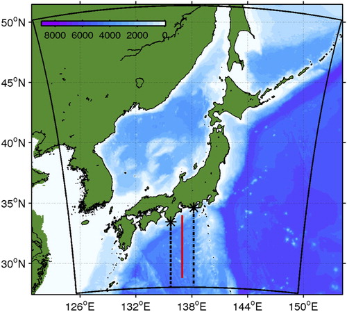
Table 1. Numerical configurations of the ROMS model.

Items	Data
Computational period	1 Jan. 2010 to 5 May 2013 (plus one year model spin-up)
Horizontal grid resolution	3 km
Grid	784×864 (× 32 vertical s-layers)
Baroclinic time step	120 s
Surface wind stress	JMA GPV-GSM (daily average, dx = 20 km)
Other surface flux	COADS05 (monthly climatology)
SST to restore	Pathfinder-AVHRR (monthly climatology)
Topography	JODC J-EGG500 supplemented by SIO SRTM30_Plus
Boundary condition	JCOPE2 (daily average, dx = 1/12^o)
Temperature and salinity nudging towards:	7-day average TUMSAT-TS (ROMS-TUM) 10-day average JCOPE2-TS (ROMS-JCP) none (ROMS-FREE)
Nudging strength	1/10 (d^−1)

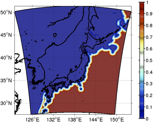
In the present study, the two types of data assimilation are examined based on the temperature and salinity nudging in ROMS with one towards time-varying three-dimensional TS fields of the JCOPE2-TS and the other towards those of the TUMSAT-TS. We call the former case ROMS-JCP and the latter ROMS-TUM. A weak nudging strength of 1/10 d⁻¹ is set in both ROMS runs. In the ROMS-JCP, the shallow coastal areas with depths less than 20 m are not included in the nudging to allow intrinsic shallow water dynamics that are not well represented in the JCOPE2 model. The TUMSAT-TS field is optimal for the offshore subsurface regions on the Pacific side of Japan because a sufficient number of Argo floats have been deployed. Therefore, the temperature and salinity fields in the coastal regions and in the Sea of Japan are supplemented by the JCOPE2-TS at the blending rate shown in Fig. 2. We also exclude surface water shallower than 80 m (z < −80 m) from the salinity nudging in ROMS-TUM because the near-surface salinity is not well quality-controlled. Note that the daily-averaged results from the models are exploited in the following analyses unless otherwise stated.

Fig. 2 The blending rate (no dimension, ranging from 0 to 1) of the TUMSAT-TS data against the JCOPE2-TS data.

b TUMSAT-TS Model

The TUMSAT-TS was derived from altimeter data and in situ density data primarily based on the method described in Takano et al. (2009). Water temperature was estimated from isothermal depths that are derived from an empirical equation based on the two-layer model of Goni et al. (1996) with altimetry absolute dynamic height acquired from Aviso data along with in situ Argo temperature profiles:(1) where ε = (ρ₂ – ρ₁)/ρ₂ so that the reduced gravity is g′ = εg; the subscripts 1 and 2 correspond to the upper and lower layers segmented by the user-defined temperature T at the interface between two layers; x, y, and t are the two horizontal coordinates and time, depending on the availability of the Aviso data; h is the thickness of the upper-layer, thus is the isothermal depth; α and β are empirical parameters to be determined; η is the absolute dynamic topography from Aviso. First, the Argo temperature and salinity profiles were used to determine ε(x₀, y₀, t₀, T) h(x₀, y₀, t₀, T) on the sparse Argo float locations available at (x₀, y₀, t₀) in the upper layer. Then α (T) and β (T) were derived from a linear regression analysis between η(x₀, y₀, t₀) and ε(x₀, y₀, t₀, T) h(x₀, y₀, t₀, T). Subsequently we evaluated the ε(x, y, t, T) distribution at the resolution of Aviso, (x, y, t), from the monthly mean climatology of temperature and salinity from the forty-first to fiftieth years of the Modular Ocean Model (MOM)-based high-resolution oceanic global circulation model for the Earth Simulator (OFES) data (Masumoto et al., 2004) instead of the sparse Argo profiles. These procedures enabled us to estimate arbitrary isothermal depth h. In particular, multiple isotherms of 3°, 5°, 10°, 16°, 17°, 18°, 20°, and 25°C were derived in the present study. Satellite SST data were used for the surface temperature. The temperature in the subsurface deeper layer with T < 3°C was replaced with monthly mean OFES temperature.

After the three-dimensional temperature field was obtained, the three-dimensional salinity field was estimated with the predetermined polynomial regression coefficients between the temperature and salinity data of Argo floats deployed in the area (20°–50°N, 136°–180°E) from 1 August 2004 to 31 December 2012. Each profile was interpolated vertically at 100 hPa intervals. The Pacific side of the study area was divided into blocks by creating 5^o × 5^o horizontal grids with 15 vertical levels (25, 50, 100, 150, 200, 300, 400, 500, 600, 700, 800, 900, 1100, 1300, and 1500 m depths). The regression analysis was conducted for each block by collecting all available Argo data in the block, removing the highest and lowest 50 temperature data points (and associated salinity data) to enhance the accuracy. The polynomial order was selected according to the Akaike information criterion. Then, to reduce blockwise discontinuity in the salinity estimate, we computed the horizontal distributions of the salinity on isotherm surfaces from −0.3° to 31°C at intervals of 0.1°C and applied horizontal bilinear interpolation and vertical linear interpolation. Even with this smoothing operation, there were still undesirable block noises in the salinity estimate (see Section 3). Note that we also excluded near-surface (z < −80 m) salinity from the TS nudging because it is not as precise as the temperature owing to the limited number of Argo profiles. As a consequence, the diagnostic three-dimensional temperature and salinity fields (viz., TUMSAT-TS) were available at seven-day intervals with a horizontal resolution of 1/10° for the present ROMS simulation.

c Measures for assessing mesoscale reproducibility

Reproducibility of the mesoscale oceanic structures in the ROMS results was measured quantitatively with root-mean-square error (RMSE) and a model skill score (e.g., Ralston, Geyer, & Lerczak, 2008; Warner, Geyer, & Lerczak, 2005; Wilmott, 1981) as represented by the following equations.(2) (3) where X_model is the ROMS model result; X_obs is the observed “true” data (e.g., from Aviso, JCOPE2, and JMA); overbars denote the averaging operation, and the summations are taken over the number of grid points where the observation is available. The RMSE has the same units as X (e.g., velocity, SSH, T, and S) and shows better agreement the closer it is to zero, while the skill is non-dimensional and a value of one indicates perfect reproducibility. Note that alternative skill scores exist, such as the one proposed by Murphy (1988), but we did not find any substantial differences in the result.

3 Validity of the TUMSAT-TS estimate

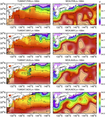
To evaluate the accuracy of the TUMSAT-TS estimate, we compared the results with the hydrography observations along 137°E conducted by the JMA. Note that the climatological time averages were taken over three years (2010–2012) for the ROMS result and ten years (1997–2010) for the JMA data for comparable accuracy using a limited number of the observations. This mismatch of the two periods does not introduce any significant error associated with interannual variability in the following analyses. The seasonally averaged stratification in summer and winter from TUMSAT-TS is in good agreement with the measurement on the whole (Fig. 3). The modelled thermocline and haloclines are slightly deeper, and the subsurface salinity minima, at around z = −1000 m, are formed more widely in the vertical than the measurements. However, except for these minor mismatches, TUMSAT-TS reproduces the stratification adequately. Horizontal distributions of the monthly climatology of temperature and salinity from TUMSAT-TS were then compared with the monthly averaged climatology from the World Ocean Atlas 2005 (WOA05; Levitus, Gurgett, & Boyer, 1994; Antonov, Locarnini, Boyer, Mishonov, & Garcia, 2006; Locarnini, Mishonov, Antonov, Boyer, & Garcia, 2006) at z = −100 m (Figs 4 and 5). The TUMSAT-TS shows fair agreement with WOA05, particularly in temperature. The zonal gradient of temperature is well reproduced in all four seasons. In contrast, the salinity field has an undesirable discontinuity at several locations, arising from the piecewise regression estimate (Section 2.b), and is underestimated, as indicated by the deeper haloclines. Moreover, warmer and fresher patches are found around the Izu Ridge (30°–34^oN and 138°–141^oE), particularly in summer. These spurious noises are artifacts of the TUMSAT-TS model due mainly to shallow topography, such as ridges, where dense water does not exist in the lower layer in the two-layer model. This leads to diminishing density differences between the two layers thus reducing ε (measure of stratification; Eq. (1)), resulting in somewhat deeper isotherm surfaces. This discrepancy in TUMSAT-TS is mediated by introducing the blending with JCOPE-TS, as shown in Fig. 2, yet it cannot be completely avoided (see Section 5 for a more a detailed argument). Nevertheless, these results suggest that although reproducibility in the stratification is moderate, the slight deviations in the vertical profiles cause nontrivial difference between the TUMSAT-TS estimate and the WOA05 data, specifically in horizontal salinity distribution. In summary, there is room for improvement in the TUMSAT-TS salinity estimate.

Fig. 3 Comparison of the seasonally averaged stratification along the JMA transect at 137°E from the TUMSAT-TS data and JMA observations for summer (upper, July–September) and winter (lower, January–March).

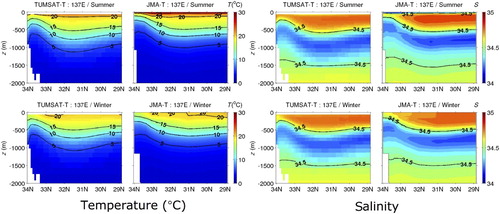
Fig. 4 Climatological monthly averaged temperature at z = −100 m for the four seasons (February, May, August, and November); (left) TUMSAT-TS data and (right) World Ocean Atlas 2005 (WOA05).

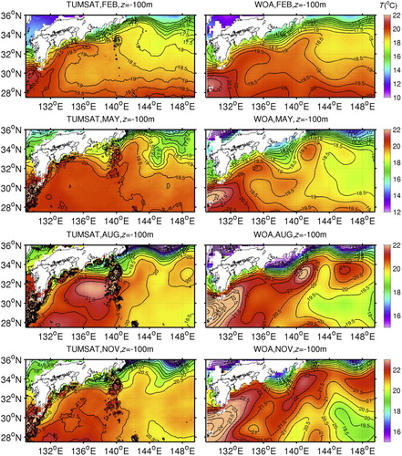
Fig. 5 As in Fig. 4, but for salinity at z = −100 m.

4 The assimilative ROMS reproducibility

The two ROMS results with temperature and salinity nudging are compared with Aviso altimeter data and the JCOPE2 reanalysis to quantitatively assess the model's reproducibility. Figure 6 shows the annually averaged surface velocity magnitude, SSH variance, and surface eddy kinetic energy (EKE) evaluated for 2012. The EKE accounts for the variability shorter than the 90-day period with the frequency high-pass filtered surface horizontal velocity¹⁴. These model-derived variables are basically consistent with the data. The mean Kuroshio paths are approximately the same, and the mesoscale variability (SSH variances) and EKE are energetic in the Kuroshio Extension region in all the results. The RMSE and skill for each year during the 2010–2012 period also represent quantitative agreement with the data for both the assimilative ROMS runs (Table 2).

Fig. 6 Annually averaged velocity magnitude at the surface (top), the SSH variance depicting the mesoscale variability (middle), and the surface eddy kinetic energy (EKE) for periods shorter than 90 days for 2012 (bottom); (left) ROMS-JCP, (middle) ROMS-TUM, and (right) Aviso data or the JCOPE2 reanalysis.

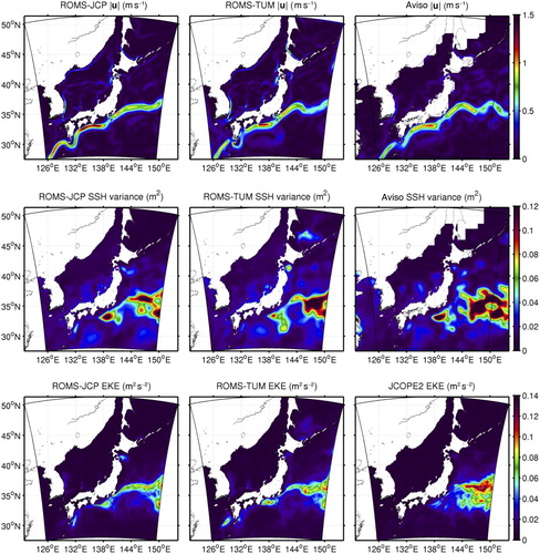
Table 2. Model skill scores (dimensionless) and RMSEs of surface velocity (m s⁻¹), SSH variance (m²), and surface eddy kinetic energy (EKE, m² s⁻²), surface kinetic energy (KE, m² s⁻²) relative to Aviso (velocity magnitude and SSH variance) or to the JCOPE2 reanalysis (EKE and KE) for the years 2010–2012.

		Surface Velocity		SSH Variance		EKE		KE
Model	Year	Skill	RMSE	Skill	RMSE	Skill	RMSE	Skill	RMSE
ROMS-JCP	2010	0.7821	0.0502	0.9818	0.0034	0.9755	0.0022	0.7496	0.0025
	2011	0.7757	0.0558	0.8907	0.0074	0.9931	0.0013	0.8627	0.0025
	2012	0.7800	0.0505	0.9373	0.0052	0.9608	0.0032	0.6511	0.0033
ROMS-TUM	2010	0.7461	0.0590	0.9671	0.0047	0.9682	0.0025	0.8354	0.0024
	2011	0.7285	0.0643	0.9117	0.0060	0.9595	0.0029	0.7722	0.0034
	2012	0.7590	0.0559	0.9434	0.0051	0.9496	0.0035	0.4013	0.0047
ROMS-FREE	2010	0.6342	0.0791	0.7852	0.0186	0.5334	0.0265	0.2618	0.0152
	2011	0.7304	0.0633	0.7707	0.0160	0.4855	0.0297	0.2675	0.0162
	2012	0.5586	0.0905	0.7079	0.0212	0.4741	0.0340	0.1742	0.0258

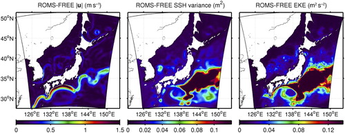
To demonstrate the substantial importance of temperature and salinity nudging, an alternative ROMS run without any assimilation, called ROMS-FREE, was carried out. Except for the exclusion of temperature and salinity nudging, the other numerical configurations in the ROMS-FREE case remained identical to the ROMS-TUM and ROMS-JCP cases. Annually averaged velocity magnitude, SSH variance, and EKE at the surface for 2012 from the ROMS-FREE are shown in Fig. 7. The path of the Kuroshio meanders unrealistically, and the SSH variance and EKE are overly energetic compared with the cases with data assimilation (Fig. 6). The result is much lower skill and poorer RMSE (Table 2) because of the underestimate of the energy dissipation due to the exclusion of temperature and salinity nudging (Uchiyama et al., 2012). These results provide the solid evidence that ensures the inevitability of the inclusion of temperature and salinity nudging for much better mesoscale reproducibility in the Kuroshio region.

Fig. 7 As in Fig. 6, but for ROMS-FREE (excluding temperature and salinity nudging).

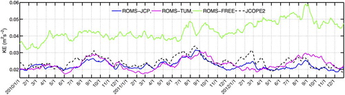
Time series of the volume-averaged surface kinetic energy (KE) in the upper ocean above z = −400 m on the Pacific side of the model domain is plotted for the two assimilative ROMS results along with the ROMS-FREE output and the JCOPE2 data (Fig. 8). The corresponding model skill and RMSE are summarized in the last two columns of Table 2. The KE behaves quite similarly for the ROMS-TUM, ROMS-JCP, and JCOPE2 cases in the first year, but after that ROMS-TUM and ROMS-JCP start deviating slightly from the JCOPE2 data, particularly in the third year. In 2011, the KE derived from ROMS-TUM is underestimated in winter, whereas it is overestimated in summer and fall. In early 2012, both ROMS-TUM and ROMS-JCP exhibit lower KE compared with JCOPE2, while ROMS-TUM deviates slightly more than ROMS-JCP in late 2012. The RMSE and skill in Table 2 partly support this trend. Both the assimilative ROMS models perform quite well in the first year after initialization although they gradually drift from the JCOPE2 data. The temperature and salinity of the TUMSAT-TS are estimated separately, which could become a source of long-term accumulated errors. In contrast, ROMS-FREE produces unrealistically large KE for the three years with the worst skill scores and RMSEs. These results demonstrate that ROMS runs with temperature and salinity nudging towards either the JCOPE2-TS or TUMSAT-TS data reproduce the mesoscale variability in the Kuroshio region reasonably well for a year or two. We should note that preliminary test simulations were performed with nudging strengths of 1/5, 1/10, and 1/20 d⁻¹ (see Section 2.a) to find that there is no substantial improvement in model skill or RMSE although using 1/10 d⁻¹ results in the best skill and RMSE of the three. The spectral nudging technique (e.g., Von Storch, Langenberg, & Feser, 2000) is used occasionally in atmospheric downscaling models, in which large-scale variability is constrained by the nudging while small-scale intrinsic variability is permitted. Such a method may be an alternative for a future approach rather than further tweaking of the nudging strength.

Fig. 8 Comparison of the volume-averaged kinetic energy (KE) in the upper ocean above z = −400 m for ROMS-JCP (blue curve), ROMS-TUM (magenta curve), ROMS-FREE (green curve), and JCOPE2 reanalysis (black dashed curve).

The modelled cross-sectional temperature and salinity fields are compared with the JMA data along the 137^oE transect for the summer and winter (Fig. 9). Again, overall consistency is confirmed in both temperature and salinity in all three cases. Similar to the input TUMSAT-TS data (Section 2.a and Fig. 3), the assimilative ROMS-TUM also produces slightly thicker thermoclines and haloclines than the observations with moderate consistency in the near-surface temperature and subsurface salinity. However, ROMS-JCP has less freshening bias in salinity at around 800 m depth, while ROMS-TUM has better agreement at this depth. The corresponding RMSE and model skill also indicate good agreement with the data; in particular, both assimilative ROMS models give comparable scores for temperature and salinity (Table 3). In turn, ROMS-FREE generally exhibits much poorer reproducibility than ROMS-JCP and ROMS-TUM.

Fig. 9 Comparison of the seasonally averaged stratification from (left) ROMS-JCP, (middle) ROMS-TUM, and (right) JMA observations, along the 137°E transect for summer (upper two rows) and winter (lower two rows).

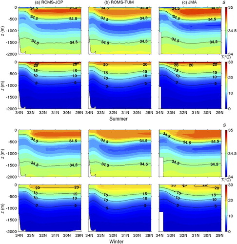
Table 3. Model skill scores (dimensionless), RMSEs of temperature, and RMSEs of salinity for the years 2010–2012 relative to JMA observations in the cross-section along the 137°E transect as shown in Fig. 9.

		Temperature		Salinity
Model	Season	Skill	RMSE (°C)	Skill	RMSE
ROMS-JCP	summer	0.9987	0.4100	0.9843	0.0350
	winter	0.9993	0.2862	0.9855	0.0331
ROMS-TUM	summer	0.9972	0.6210	0.9845	0.0378
	winter	0.9993	0.4514	0.9862	0.0350
ROMS-FREE	summer	0.9947	0.7889	0.9281	0.0671
	winter	0.9972	0.5710	0.9380	0.0621

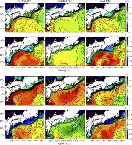
Next, monthly averaged horizontal density structures for the two assimilative ROMS results are compared with those for the JCOPE2. Figure 10 depicts the temperature and salinity distributions at z = −100 m for February and August 2012 in the Kuroshio region. The temperatures from the two ROMS cases are again in good agreement with those from JCOPE2, but the ROMS-TUM salinity is less consistent with the JCOPE2 salinity. The ROMS-TUM salinity has a weaker meridional gradient with much less freshening in the coastal area on the left side of the Kuroshio axis than the ROMS-JCP and JCOPE2 salinity. In addition, the ROMS-TUM salinity in the southern part of the domain (south of 32°N) is lower by about 0.2 than in the other two cases, leading to a weaker northeastward gradient, particularly in February. The coastal inconsistency in the temperature and salinity fields is attributed to a deficiency in the Argo floats and the altimetry data.

Fig. 10 Comparison of monthly averaged temperature and salinity in the Kuroshio region at z = −100 m from (left) ROMS-JCP, (middle) ROMS-TUM, and (right) the JCOPE2 reanalysis, for February 2012 (upper two rows) and August 2012 (lower two rows).

5 Reproducibility of the Kuroshio

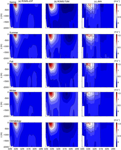
Figure 11 shows the eastward velocity normal to the 137°E cross-section for the two ROMS cases along with the geostrophic velocity estimated from in situ JMA hydrography data (see Fig. 9). All four seasonal and annual mean velocity distributions show good agreement with the JMA data in terms of the position of the Kuroshio axis approximated by the maximum velocity that appears at z > −500 m and peaks near the surface at around 33°N. The two ROMS runs, especially ROMS-TUM, indicate greater maximum eastward velocity around the Kuroshio axis than the JMA data. This is partly because of the difference in the duration of the time average between the model and the observations (Section 3). The approximate area of the Kuroshio main body in ROMS-TUM is more widely distributed both in the offshore and vertical directions. In turn, ROMS-TUM yields negative (westward) velocity far into the sea around 30°­–31°N. The ROMS-JCP also yields a westward but lower velocity but with a smaller value.

Fig. 11 Seasonally (upper four rows) and climatologically (bottom row) averaged eastward velocity normal to the 137°E cross-section from (left) ROMS-JCP, (middle) ROMS-TUM, and (right) the geostrophic velocity estimated with JMA hydrographic data. The contour interval is 0.2 m s⁻¹.

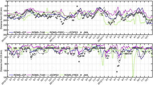
Subsequently, for more rigorous mesoscale Kuroshio modelling, the reproducibility of the transient Kuroshio path is quantitatively examined. We introduce the southward distances to the Kuroshio axis from Cape Omaezaki (CO; along about 138.20^oE, the black dotted line on the right in Fig. 1) and from Cape Shionomisaki (CS; along about 135.76°E, the black dotted line on the left in Fig. 1) to investigate the time-dependent behaviour of the position of the Kuroshio. According to the JMA, the Kuroshio axis is defined as the lateral point with maximum normal velocity at 50 m depth. Figure 12 shows two time series plots of the distance from CO and CS from the two assimilative ROMS runs, ROMS-FREE, JCOPE2, and JMA's model estimate. The ROMS-TUM, ROMS-JCP, and JCOPE2 behave quite similarly, whereas the Kuroshio path in ROMS-TUM tends to have a slightly shorter distance to the capes than the others. The ROMS-FREE performs reasonably well, except for large deviations in the later years.

Fig. 12 Temporal variations of the Kuroshio axis as a function of distance from Cape Omaezaki (CO; upper panel) and Cape Shionomisaki (CS; lower panel) for ROMS-JCP (blue curve), ROMS-TUM (magenta curve), ROMS-FREE (green curve), the JCOPE2 reanalysis (black dashed curve), and JMA's estimate (open circles).

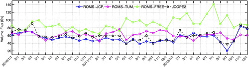
To further quantify the reproducibility of the Kuroshio, the cross-sectionally integrated eastward volume fluxes along the 137°E transect are plotted in Fig. 13 for the two assimilative ROMS cases, ROMS-FREE, and JCOPE2. The integral is taken from the bottom to the surface between 32° and 33.5°N, where the fluctuating Kuroshio axis is mainly located. The ROMS-TUM, ROMS-JCP, and JCOPE2 have similar variability, ranging from 53 to 60 Sv (1 Sv = 10⁶m³s⁻¹) that is consistent with measurement (e.g., Nitani, 1972; Qiu & Joyce, 1992). In 2010 and 2012, the fluxes from the three cases agree quite well except for April 2010 and the second half of 2012. The ROMS-TUM tends to yield slightly larger fluxes, while ROMS-JCP slightly underestimates the fluxes compared with JCOPE2, which is consistent with the cross-sectional velocity distributions in Fig. 10. In turn, the volume flux is overestimated by ROMS-FREE, ranging from 70 to 140 Sv, with degraded performance in the later years.

Fig. 13 Temporal variations of the volume flux (Sv) associated with the Kuroshio for ROMS-JCP (blue curve), ROMS-TUM (magenta curve), ROMS-FREE (green curve), and the JCOPE2 reanalysis (black dashed curve). The cross-sectional integral is taken along 137°E and between 32°N and 33.5°N.

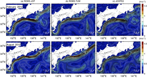
Monthly averaged, near-surface velocity vectors and their magnitude at z = −100 m for February and August 2012 are displayed in Fig. 14. The velocity field around the Kuroshio axis from ROMS-TUM agrees well with that from JCOPE2, while the ROMS-JCP results in a slightly more energetic Kuroshio with a more confined narrow main path, which is consistent with the sharpness of the density gradient in the Kuroshio front (Figs 3, 9, and 10). In addition, a recurring westward current emerges in the southern section of the Kuroshio path, most prominently in ROMS-TUM (Figs 11 and 14). This westward countercurrent varies spatially with time but appears consistently throughout the computational period. The countercurrent is more apparent in summer, corresponding to the warm-core gyre in ROMS-TUM (Fig. 10) but is weaker in winter. As we have found in the cross-sectional plots along the 137^oE transect (Fig. 11), the velocity of the countercurrent is westward down to about 800 m depth.

Fig. 14 Monthly averaged near-surface velocity vectors and their magnitude (colour) at z = −100 m for February 2012 (upper panels) and August 2012 (lower panels) for (a) ROMS-JCP, (b) ROMS-TUM, and (c) the JCOPE2 reanalysis.

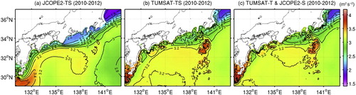
Because the countercurrent may be associated with artifacts arising from TUMSAT-TS input data (Section 3), we compared the dynamic height anomaly derived from TUMSAT-TS and JCOPE2-TS, as well as from the two ROMS runs. The dynamic height anomaly at a given pressure P, ΔD(P), is computed as(4) where P₀ = −ρ₀ gz_r; z_r is the reference depth (–100 m); ρ₀ = 1000 kg m⁻³; g is acceleration due to gravity (9.81 m s⁻²); ρ₁ is the density at z_r; ρ₂ is the reference density at T = 0°C and S = 35. Figure 15 shows the dynamic height anomaly computed using ROMS-JCP, ROMS-TUM, and JCOPE2-TS data averaged monthly for February and August 2012. The dynamic height anomaly ΔD is similarly distributed in winter, whereas a discrepancy is prominent in summer. In August, all three cases induce the pressure gradient force (PGF) that promotes the northeastward-drifting Kuroshio in a wide area. However, the along-shelf cross-frontal PGF of ROMS-TUM is weaker than that for the other two cases. The offshore ΔD for ROMS-TUM has a high centred on the Izu Ridge (at 140.2°E, 32.8°N), which is consistent with the density field (Fig. 10), promoting the clockwise gyre and thus the westward countercurrent to the south (Figs 11 and 14). To compare with the forcing field associated with the nudging, ΔD computed with TUMSAT-TS data is plotted in Fig. 16. Irregularity in ΔD is found around the Izu Ridge, particularly in summer, attributable to the warmer and fresher patches existing in TUMSAT temperature (Fig. 4) and salinity (Fig. 5). Figure 17 shows the three-year average ΔD calculated with JCOPE2-TS, TUMSAT-TS, and a combination of TUMSAT temperature and JCOPE2 salinity. Again, the weaker along-shelf cross-frontal PGF and the larger ΔD bias are pronounced using the TUMSAT density estimate. Nevertheless, the apparent similarity in Figs 17b and 17c suggests that salinity is much less influential in ΔD, indicating that the TUMSAT salinity estimate with the climatological regression using Argo data does not hinder reproducibility. In summary, although TUMSAT-TS leads to good reproducibility, the modest reproducibility in the temperature estimate near the ridge causes the somewhat inaccurate large-scale horizontal flow (Fig. 14), as well as the local bias in the cross-sectional density and current structure (Figs 9 and 11), particularly in summer. However, the discrepancy is minor compared with the robust and excellent mesoscale reproducibility of ROMS-TUM over the non-assimilative ROMS-FREE model demonstrated throughout the paper.

Fig. 15 Monthly averaged dynamic height anomaly (m² s⁻²) at z = −100 m derived using (left) ROMS-JCP, (middle) ROMS-TUM, and (right) JCOPE2 data for February (upper panels) and August (lower panels) 2012.

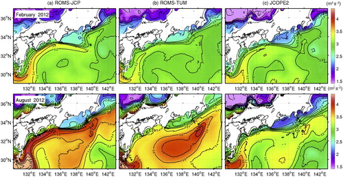
Fig. 16 As in Fig. 15, but with TUMSAT-TS for (a) February and (b) August 2012.

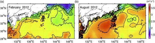
Fig. 17 As in Fig. 15, but using (a) JCOPE2-TS, (b) TUMSAT-TS data, and (c) a combination of TUMSAT-T and JCOPE2-S data, averaged over the three-year computational period.

6 Summary and discussion

The TUMSAT-TS dataset was acquired using the empirical method for estimating three-dimensional oceanic thermal structure proposed by Takano et al. (2009), along with a piecewise regression analysis between temperature and salinity using Argo profiling data. Because this new density estimate uses only currently available data, there is no new cost for instrumentation. At first, TUMSAT-TS data were examined by comparison with in situ hydrography. Although the temperature structure agrees well with observations, the salinity does not indicate a fully satisfactory three-dimensional structure. Subsequently, a twin ROMS downscaling experiment was conducted with temperature and salinity nudging (or robust diagnosis), which is essential for reproducing the Kuroshio variability realistically. Weak nudging towards (i) TUMSAT-TS (ROMS-TUM) and towards (ii) the JCOPE2-TS reanalysis (ROMS-JCP) was conducted for quantitative comparison.

A comprehensive assessment was carried out on the model results with the 3D-Var embedded assimilative JCOPE2 reanalysis, the Aviso SSH, and JMA's in situ hydrographic data. The RMSE and model skill score were utilized for quantitative measure of the models’ reproducibility. Both assimilative ROMS models produced good model skill scores and low RMSEs in the surface velocity, SSH variance, surface EKE, stratification, transient migration of the Kuroshio path, and the volume flux due to the Kuroshio, at least for one or two years after the model's initialization, excluding the one-year spin-up. On the other hand, a supplemental ROMS run without assimilation (ROMS-FREE model) totally failed to replicate the upper ocean dynamics. Therefore, the newly proposed TUMSAT-TS density estimate is potentially a powerful dataset for improving mesoscale reproducibility in the oceanic reanalysis.

Nevertheless, TUMSAT-TS has some deficiencies and needs to be further modified and corrected. The salinity structure and halocline depth moderately agree with JMA data along the 137°E transect. This slight error in TUMSAT salinity produced inaccurate horizontal subsurface salinity distribution, whereas it did not impede the mesoscale reproducibility substantially. As Ji et al. (2000) and Troccoli et al. (2002) suggested, both the temperature and salinity fields should be used simultaneously for successful assimilative oceanic reanalysis to avoid density artifacts. In this sense, the proposed empirical salinity estimate based on the regression works reasonably well in maintaining overall reproducibility. On the other hand, a satellite sea surface salinity measurement, such as that from the Aquarius/Satélite de Aplicaciones Científicas (SAC)-D mission (e.g., Lagerloef, Swift, & Le Vine, 1995), and an increased number of deployed Argo floats are prospective in situ datasets for supplementing the salinity estimate. In turn, undesirable dynamic height distribution, thus, erroneous PGF appears, particularly in summer, to promote spurious westward drifting countercurrents to the south of the Kuroshio, mainly because of inaccurate temperature estimates near the ridge. Therefore, there is room for improvement for the quality of both the temperature and salinity estimates although the proposed TUMSAT-TS estimate has proven to be a strong candidate for the dataset to be used in assimilative mesoscale oceanic downscaling modelling even if reliable reanalyses, such as the JCOPE2 data, were unavailable.

It is worth mentioning that we have conducted similar downscaling JCOPE2-ROMS modelling runs nudged towards JCOPE-TS data to examine mesoscale reproducibility for the Japan Sea (Uchiyama, Miyazaki, Kanki, & Miyazawa, 2015) and the East China Sea (Kamidaira et al., 2017). Good agreement with satellite and in situ data was exhibited, comparable to the results demonstrated here. Therefore, as long as TUMSAT-TS is reliably produced with a sufficient amount of Argo data, we may expect successful reanalyses in regions other than the Kuroshio region off Japan that was investigated in the present study. In addition, TUMSAT-TS may be exploited for regional ocean models with other assimilation techniques, such as the widely used 3D-Var, which requires careful investigations a priori for estimating error covariance and decorrelation length scale to avoid interpolation artifacts inherent in TUMSAT-TS data.

This study focused on a high-resolution ROMS that fully resolves mesoscale eddies but under-resolves submesoscale coherent structures (SCSs). We expect that higher resolution models should, in principle, represent eddies, fronts, and filaments more adequately. However, this is not the case for the Kuroshio region studied here. At a horizontal resolution of 3 km, ROMS-FREE significantly overestimated the meandering of the path of the Kuroshio, which results in a serious mismatch with the data, as shown in Figs 7, 8, 12, and 13, even though the resolved eddies are seemingly quite realistic (not shown). At further downscaling to a lateral resolution of 1 km, the behaviour of the Kuroshio becomes much closer to that of JCOPE2, even without temperature and salinity nudging (Uchiyama et al., 2012). This implies that if the model represents SCSs well, then it spontaneously stabilizes the Kuroshio through vigorous energy dissipation due to SCSs. TS nudging works adequately as if subgrid-scale eddy-induced mixing had been imposed, where the energy contained in the available potential energy, KE, and EKE is appropriately extracted through forward energy cascade to dissipation.

Disclosure statement

No potential conflict of interest was reported by the authors.

ORCID

Yusuke Uchiyama http://orcid.org/0000-0002-2234-3608

Additional information

Funding

YU and HY appreciate the financial support from Japan Science and Technology Agency Core Research for Evolutional Science and Technology (JST-CREST) program [grant number JPMJCR12A6]. YU also offers thanks for the support from the Japan Society for the Promotion of Science (JSPS) Grant-in-Aid for Scientific Research [grant number 24560622], [grant number 15H04049], [grant number 15H00977], and [grant number 15KK0207].

Notes

1 http://www.aviso.altimetry.fr/en/home.html

2 http://www.jamstec.go.jp/J-ARGO/index_e.html

3 http://www-hrx.ucsd.edu/

4 http://www.pmel.noaa.gov/tao/index.shtml

5 http://www.argo.net

6 http://www.jamstec.go.jp/jcope/htdocs/e/home.html

7 http://web.atmos.ucla.edu/roms/Welcome.html

8 https://www.myroms.org/

9 http://topex.ucsd.edu/WWW_html/srtm30_plus.html

10 http://www.jodc.go.jp/data_set/jodc/jegg_intro_j.html

11 http://www.jmbsc.or.jp/jp/online/file/f-online10100.html

12 http://iridl.ldeo.columbia.edu/SOURCES/.COADS/

13 http://podaac.jpl.nasa.gov/AVHRR-Pathfinder

14 There has been an argument on possible errors associated with frequency filters for the multiscale Reynolds decomposition (Liang, 2016).

References

- Antonov, J. I., Locarnini, R. A., Boyer, T. P., Mishonov, A. V., & Garcia, H. E. (2006). Salinity. In S. Levitus, (Ed.), World ocean atlas 2005, Vol. 2, NOAA atlas NESDIS 62. Washington, DC: U.S. Government Printing Office.
- Argo Science Team. (2001). Argo: The global array of profiling floats. In C. J. Koblinsky, & N. R. Smith (Eds.), Observing the oceans in the 21st century (pp. 248–258). Melbourne: GODAE Project Office and Bureau of Meteorology.
- Becker, J. J., Sandwell, D. T., Smith, W. H. F., Braud, J., Binder, B., Depner, J., … Weatherall, P. (2009). Global bathymetry and elevation data at 30 arc seconds resolution: SRTM30_PLUS. Marine Geodesy, 32(4), 355–371. doi: 10.1080/01490410903297766
- Behringer, D. W., Ji, M., & Leetmaa, A. (1998). An improved coupled model for ENSO prediction and implications for ocean initialization. Part I: The ocean data assimilation system. Monthly Weather Review, 126, 1013–1021. doi: 10.1175/1520-0493(1998)126<1013:AICMFE>2.0.CO;2
- Buijsman, M., Uchiyama, Y., McWilliams, J. C., & Hill-Lindsay, C. R. (2012). Modeling semiduirnal internal tides in the Southern California Bight. Journal of Physical Oceanography, 42, 62–77. doi: 10.1175/2011JPO4597.1
- Durski, S. M., Glenn, S. M., & Haidvogel, D. B. (2004). Vertical mixing schemes in the coastal ocean: Comparison of the level 2.5 Mellor-Yamada scheme with an enhanced version of the K profile parameterization. Journal of Geophysical Research, 109, C01015. doi: 10.1029/2002JC001702
- Fujii, Y., & Kamachi, M. (2003). A reconstruction of observed profiles in the sea east of Japan using vertical coupled temperature–salinity EOF modes. Journal of Oceanography, 59, 173–186. doi: 10.1023/A:1025539104750
- GODAE. (2001). Strategic plan. GODAE report No. 6, GODAE International Project Office. Melbourne: Bureau of Meteorology.
- Goni, G., Kamholz, S., Garzoli, S., & Olson, D. (1996). Dynamics of the Brazil-Malvinas Confluence based on inverted echo sounders and altimetry. Journal of Geophysical Research: Oceans, 101, 16273–16289. doi: 10.1029/96JC01146
- Guinehut, S., Larnicol, G., & Le Traon, P.-Y. (2002). Design of an array of profiling floats in the North Atlantic from model simulations. Journal of Marine Systems, 35, 1–9. doi: 10.1016/S0924-7963(02)00042-8
- Guinehut, S., Le Traon, P.-Y., Larnicol, G., & Philipps, S. (2004). Combining Argo and remote-sensing data to estimate the ocean three-dimensional temperature fields—A first approach based on simulated observation. Journal of Marine Systems, 46, 85–98. doi: 10.1016/j.jmarsys.2003.11.022
- Hayes, S. P., Mangum, L. J., Picaut, J., Sumi, A., & Takeuchi, K. (1991). TOGA-TAO: A moored array for real-time measurements in the tropical Pacific Ocean. Bulletin of the American Meteorological Society, 72, 339–347. doi: 10.1175/1520-0477(1991)072<0339:TTAMAF>2.0.CO;2
- Ji, M., Reynolds, R. W., & Behringer, D. W. (2000). Use of TOPEX/Poseidon sea level data for ocean analyses and ENSO prediction. Some early results. Journal of Climate, 13, 216–231. doi: 10.1175/1520-0442(2000)013<0216:UOTPSL>2.0.CO;2
- Kamachi, M., Kuragano, T., Ichikawa, H., Nakamura, H., Nishina, A., Isobe, A., … Uboldi, F. (2004). Operational data assimilation system for the Kuroshio South of Japan: Reanalysis and validation. Journal of Oceanography, 60, 303–312. doi: 10.1023/B:JOCE.0000038336.87717.b7
- Kamachi, M., Kuragano, T., Yoshioka, N., Zhu, J., & Uboldi, F. (2001). Assimilation of satellite altimetry into a western North Pacific operational model. Advances in Atmospheric Sciences, 18, 767–786.
- Kamidaira, Y., Uchiyama, Y., & Mitarai, S. (2017). Eddy-induced transport of the Kuroshio warm water around the Ryukyu Islands in the East China Sea. Continental Shelf Research, 143, 206–218. doi: 10.1016/j.csr.2016.07.004
- Lagerloef, G. S. E., Swift, C. T., & Le Vine, D. M. (1995). Sea surface salinity: The next remote sensing challenge. Oceanography, 8, 44–50. doi: 10.5670/oceanog.1995.17
- Large, W. G., McWilliams, J. C., & Doney, S. C. (1994). Oceanic vertical mixing: A review and a model with a nonlocal boundary layer parameterization. Reviews of Geophysics, 32, 363–403. doi: 10.1029/94RG01872
- Levitus, S., Gurgett, R., & Boyer, T. P. (1994). Salinity. In S. Levitus (Ed.), World ocean atlas 1994, Vol. 3, NOAA atlas NESDIS 3. Washington, DC: U.S. Government Printing Office.
- Liang, X. S. (2016). Canonical transfer and multiscale energetics for primitive and quasigeostrophic atmospheres. Journal of the Atmospheric Sciences, 73, 4439–4468. doi: 10.1175/JAS-D-16-0131.1
- Locarnini, R. A., Mishonov, A. V., Antonov, J. I., Boyer, T. P., & Garcia, H. E. (2006). Temperature. In S. Levitus (Ed.), World ocean atlas 2005, Vol. 1, NOAA atlas NESDIS 61. Washington, DC: U.S. Government Printing Office.
- Mason, E., Molemaker, J., Shchepetkin, A. F., Colas, F., McWilliams, J. C., & Sangrà, P. (2010). Procedures for offline grid nesting in regional ocean models. Ocean Modelling, 35, 1–15. doi: 10.1016/j.ocemod.2010.05.007
- Masumoto, Y., Sasaki, H., Kagimoto, T., Komori, N., Ishida, A., Sasai, Y., … Yamagata, T. (2004). A fifty-year eddy-resolving simulation of the world ocean—preliminary outcomes of OFES (OGCM for the Earth Simulator). Journal of the Earth Simulator, 1, 35–56.
- McPhaden, M. J. (1993). TOGA-TAO and the 1991–93 El Niño–Southern Oscillation event. Oceanography, 6(2), 36–44. doi: 10.5670/oceanog.1993.12
- Miyazawa, Y., Zhang, R., Guo, X., Tamura, H., Ambe, D., Lee, J.-S., … Komatsu, K. (2009). Water mass variability in the western North Pacific detected in a 15-year eddy resolving ocean reanalysis. Journal of Oceanography, 65, 737–756. doi: 10.1007/s10872-009-0063-3
- Murphy, A. H. (1988). Skill scores based on the mean square error and their relationships to the correlation coefficient. Monthly Weather Review, 116, 2417–2424. doi: 10.1175/1520-0493(1988)116<2417:SSBOTM>2.0.CO;2
- Nitani, H. (1972). Beginning of the Kuroshio. In H. Stommel, & Y. K (Eds.), Kuroshio- Its physical aspects (pp. 129–163). Tokyo: University of Tokyo Press.
- Qiu, B., & Joyce, T. M. (1992). Interannual variability in the mid- and low-latitude western North Pacific. Journal of Physical Oceanography, 22, 1062–1079. doi: 10.1175/1520-0485(1992)022<1062:IVITMA>2.0.CO;2
- Ralston, D. K., Geyer, W. R., & Lerczak, J. A. (2008). Subtidal salinity and velocity in the Hudson River estuary: Observations and modeling. Journal of Physical Oceanography, 38, 753–770. doi: 10.1175/2007JPO3808.1
- Shchepetkin, A. F., & McWilliams, J. C. (2005). The Regional Oceanic Modeling System (ROMS): A split-explicit, free-surface, topography-following-coordinate oceanic model. Ocean Modelling, 9, 347–404. doi: 10.1016/j.ocemod.2004.08.002
- Shchepetkin, A. F., & McWilliams, J. C. (2008). Computational kernel algorithms for fine-scale, multiprocess, longtime oceanic simulations. In R. Temam, & J. Tribbia (Eds.), Handbook of numerical analysis: Computational methods for the ocean and the atmosphere (pp. 119–181). Amsterdam: Elsevier.
- Takano, A., Yamazaki, H., Nagai, T., & Honda, O. (2009). A method to estimate three-dimensional thermal structure from satellite altimetry data. Journal of Atmospheric and Oceanic Technology, 26, 2655–2664. doi: 10.1175/2009JTECHO669.1
- Troccoli, A., Balmaseda, M. A., Segschneider, J., Vialard, J., Anderson, D. L. T., Haines, K., … Fox, A. D. (2002). Salinity adjustments in the presence of temperature data assimilation. Monthly Weather Review, 130, 89–102. doi: 10.1175/1520-0493(2002)130<0089:SAITPO>2.0.CO;2
- Uchiyama, Y., Idica, E. Y., McWilliams, J. C., & Stolzenbach, K. D. (2014). Wastewater effluent dispersal in southern California bays. Continental Shelf Research, 76, 36–52. doi: 10.1016/j.csr.2014.01.002
- Uchiyama, Y., Ishii, S., & Miyazawa, Y. (2012). Ocean downscaling effects on the Kuroshio Extension Jet using a JCOPE2-ROMS system. Journal of Japan Society of Civil Engineers, Series B2, 68(2), 436–440. doi:10.2208/kaigan.68.I_436. (in Japanese with English abstract).
- Uchiyama, Y., Miyazaki, D., Kanki, R., & Miyazawa, Y. (2015). Effects of submesoscale eddies on seasonal variability of the Subpolar Front and the Tsushima warm current in the Japan Sea. Journal of Japan Society of Civil Engineers, Series B2, 71(2), 415–420. doi:10.2208/kaigan.71.I_415. (in Japanese with English abstract).
- Uchiyama, Y., Suzue, Y., & Yamazaki, H. (2017). Eddy-driven nutrient transport and associated upper-ocean primary production along the Kuroshio. Journal of Geophysical Research: Oceans, 122, 5046–5062. doi: 10.1002/2017JC012847
- Von Storch, H., Langenberg, H., & Feser, F. (2000). A spectral nudging technique for dynamical downscaling purposes. Monthly Weather Review, 128, 3664–3673. doi: 10.1175/1520-0493(2000)128<3664:ASNTFD>2.0.CO;2
- Warner, J. C., Geyer, W. R., & Lerczak, J. A. (2005). Numerical modeling of an estuary: A comprehensive skill assessment. Journal of Geophysical Research, 110, C05001. doi: 10.1029/2004JC002691
- Wilmott, C. J. (1981). On the validation of models. Physical Geography, 2, 184–194. doi: 10.1080/02723646.1981.10642213
- Wunsch, C. (2001). Ocean observations and the climate forecast problem. In R. P. Pearce (Ed.), Meteorology at the millennium (pp. 217–224). London: Academic Press.