A Study of the Impact of the Fukushima Nuclear Leak on East China Coastal Regions

ABSTRACT

The nuclear leak in Fukushima, Japan, which occurred on 11 March 2011, had disastrous impacts in many regions of the northern hemisphere. In this study, a highly resolved, one-way nesting model incorporating tides is set up with the Regional Ocean Modeling System (ROMS) to simulate and predict the potential impact of the disaster on the East China Sea (ECS), with the large domain covering the entire North Pacific. Of the four main waterways, namely Taiwan Strait, the waterway east of Taiwan, Tokara Strait, and Tsushima Strait, the first two have net fluxes of radionuclides into the ECS, while the other two have net outward transport during the entire 14-year period of the simulation (2011–2025). Differing from previous studies, we have taken into account background radionuclides in this model; the results agree well with available observations. Based on the simulation, the radioactive material has arrived in the ECS. The amount will reach its peak in 2019 and late in 2021 will return to its original state before the accident. Temporally it has a clear seasonal variability, with peaks usually appearing during winter. Spatially it is not homogeneously distributed, and the concentration has local maxima along the coasts of Jiangsu and Zhejiang, which are the most populous regions of China; a conspicuous feature is the Subei Bank high in summer. This study is expected to help form policy for rapid response to such disasters.

RÉSUMÉ

[Traduit par la rédaction] La fuite radioactive qui s’est produite le 11 mars 2011, à Fukushima, au Japon, a eu des conséquences désastreuses dans de nombreuses régions de l’hémisphère Nord. Pour cette étude, nous exploitons une simulation à haute résolution d’un modèle à imbrication unidirectionnelle comprenant les marées ainsi qu’un système de modélisation océanique régional (ROMS), afin de simuler et de prévoir l’impact potentiel du désastre sur la mer de Chine orientale, et ce, sur un domaine étendu couvrant la totalité du Pacifique Nord. Des quatre voies navigables principales, notamment le détroit de Taiwan, le chenal à l’est de Taiwan, le détroit de Tokara et le détroit de Tsushima, les deux premières génèrent des flux nets de radionucléides vers la mer de Chine orientale, tandis que les deux autres produisent un transport net hors de celle-ci durant les 14 années de la période de simulation (2011–2025). Contrairement aux études précédentes, nous avons tenu compte, dans le modèle, des radionucléides de fond. Les résultats concordent avec les observations disponibles. D’après la simulation, des matières radioactives ont atteint la mer de Chine orientale. Leurs concentrations atteindront un maximum en 2019. Vers la fin de 2021, elles retourneront à leur état normal avant accident. Elles présentent une variabilité saisonnière évidente, avec des pics apparaissant généralement en hiver. Sur le plan spatial, les concentrations ne sont pas distribuées de façon homogène et montrent des maximums locaux le long des côtes du Jiangsu et du Zhejiang, qui sont les régions les plus peuplées de Chine. Le maximum estival du banc de Subei est aussi notable. Nous espérons que cette étude servira à mettre en œuvre des politiques d’intervention rapide en cas de désastres semblables.

KEYWORDS:

• Fukushima nuclear accident
• East China Sea
• one-way nesting

1 Introduction

An earthquake of magnitude 9.0 and the subsequent tsunami with waves of 16 m nearshore to Fukushima, Japan, on 11 March 2011, severely damaged the tsunami barriers and destroyed some buildings (Tohoku Earthquake Tsunami Joint Survey Group, 2011). The most disastrous damage was to the Fukushima Dai-ichi Nuclear Power Plant; venting of gases and vapour blasts that occurred outside the reactors led to the emission of radioactive materials into the air and coastal waters (Aoyama, Uematsu, Tsumune, & Hamajima, 2013; Buesseler, Aoyama, & Fukasawa, 2011). This was the Fukushima Dai-ichi Nuclear Power Plant accident or, more simply, the Fukushima accident. Fortunately, the reactors were not completely damaged as happened at Chernobyl (Leon et al., 2011). This accident was, therefore, not as severe as the Chernobyl accident, which had a widespread influence on Europe, Asia, and North America (Povinec et al., 1988), with a total radionuclide emission up to 13,000 PBq (1PBq = 1015 Bq) (Saenko et al., 2011).

Although it is claimed that the release of radionuclides into the atmosphere and oceans has come to a halt, the influence of the accident, especially on the oceans, persists and will remain for a long time (Hirose, 2012; Lai, Chen, Beardsley, & Lin, 2013). According to observations from the International Atomic Energy Agency (IAEA), by July 2011 the concentration of ¹³⁷Cs in the coastal waters off Japan was more than 10,000 times higher than that measured in 2010 (Buesseler et al., 2011), and by October 2014, the concentration was still as high as 100 times the 2010 level.

From the reports issued by the Japanese local government, ¹³¹I (half-life τ = 8.02 days), ¹³⁴Cs (τ = 2.06 years), and ¹³⁷Cs (τ = 30 years) were the dominant radionuclides in monthly deposition samples, whereas ^129mTe (τ = 33.6 days), ¹²⁹Te (τ = 69.6 months), ¹³⁶Cs (τ = 35 days), ^110mAg (τ = 250 days), ⁹⁵Zr (τ = 64 days), ⁹⁵Nb (τ = 35 days), ¹⁴⁰Ba (τ = 12.7 days), and ¹⁴⁰La (τ = 1.68 days) were detected as secondary radionuclides within 300 km of the Fukushima Plant (Hirose, 2012; MEXT, 2012). As the radionuclide with the longest life cycle, ¹³⁷Cs naturally became the pollutant of most concern. However, the estimate of the total amount of ¹³⁷Cs released remains controversial. It has been estimated that the release of ¹³⁷Cs into the atmosphere is in the range of 13–15 PBq (Masamichi et al., 2011), and the amount released directly into the ocean is from 2.3 to 27 PBq (Bois et al., 2012; Kawamura et al., 2011; Tsumune, Tsubono, Aoyama, & Hirose, 2012).

The ¹³⁷Cs pollutant has been spread widely by atmospheric and oceanic circulation. It was reported that the radionuclides emitted into the atmosphere from the damaged Fukushima Plant arrived at the west coast of North America within just four days (Takemura et al., 2011). Seawater monitoring in the Northwest Pacific in May–June 2012 revealed a maximum ¹³⁷Cs concentration at 200 m depth (Wu, Zhou, & Dai, 2013), and simulations indicate that the radionuclides may reach the US coast within four to five years (Behrens, Schwarzkopf, Lübbecke, & Böning, 2012; Nakano & Povinec, 2012); after that, the radionuclides will be carried westward by the equatorial current and are expected to reach the Philippines in ten years, exerting an impact on East Asian and Southeast Asian countries.

In this study, we focus on the potential impact of the accident on China, particularly on the East China coast. Previously it has been shown that essentially no radionuclides will be transported to the China Seas (Wang, Wang, Zhu, Wang, & Liu, 2012). However, Zhao, Qiao, Wang, Xia, and Jung (2014) reported that ¹³⁷Cs had already started to intrude into the China Seas as of 2013 and, by their prediction, the concentration will increase gradually in the following five to six years. Similar results were obtained by Rong, Xu, Liang, and Zhao (2016). It should be mentioned that, because of the scarcity of data, in previous modelling efforts background ¹³⁷Cs distributions were not considered. Rong et al. (2016) made a preliminary attempt to include the background distributions but that study used only a coarsely resolved model for the entire North Pacific, and tides were not considered. How the pollutants that intrude into the East China Sea (ECS) may move, evolve, reside, or disappear is still unclear. Here we use a two-domain, one-way nesting, highly resolved (1/24° in space, 90 s in time) ocean model to simulate the intrusion and evolution of the radionuclides, with the background concentration, as well as in situ observational data assimilated, in the hope of achieving a reliable forecast. In the following, we first give a brief introduction of the model configuration and the data assimilation strategy. In Section 3, the model is validated and compared with existing studies. Section 4 presents the model results for the ECS; also presented is the potential impact of the accident. Our study is summarized in Section 5.

2 Model setup

a Model Configuration

We used the Regional Ocean Modeling System (ROMS) and adopted a two-domain, one-way nesting strategy to fulfill the simulation and prediction. As shown in Fig. 1a, the outer domain (L0) covers the entire North Pacific from the equator to Bering Strait with a coarse resolution, and the inner domain (L1; red box) zooms in on the ECS. In choosing this configuration, the open boundary problem was reduced to an acceptable level. For example, at the northern boundary of L0, there is only a shallow and narrow open channel (40 m deep and 42 km wide; i.e., the Bering Strait) that connects the North Pacific to the Arctic; we set it as closed. Another open boundary (i.e., the equator) can be viewed as closed to many dynamical processes; we also set it to closed. The horizontal resolution for the L0 domain is 1/8° × 1/8°, and for L1 it is 1/24° × 1/24°. Both the coarse- and fine-resolution models have 22 σ-levels in the vertical. The bathymetry is derived from the Earth Topography 1-arc-min (ETOPO1) model from the National Geophysical Data Center (NGDC (2015)). Table 1 provides a list of the model parameters.

Fig. 1 (a) Bathymetry (m) for the two-domain, one-way nesting model. The yellow and green dots mark the stations for OA, and the red ones are those listed in Table 6 for validation. The red box indicates the inner domain (L1). (b) Enlarged view of the ECS, namely, L1. The sections where the fluxes are calculated are shown. A: Taiwan Strait, B: East of Taiwan, C: Ishigaki to Naha, D: Naha to Amami, E: Tokara Strait, F: Tsushima Strait, G: from Ishigaki northward to 27.5°N. Also marked is a section of the East China coast (dashed purple line).

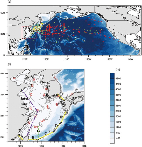
Table 1. Parameters for the two-domain nested ROMS model.

Domain	Maximum Depth (m)	Minimum Depth (m)	Latitude (°N)	Longitude (°E)	Resolution (km)	Time Step (s)
L0	5000	15	0–68	96–288	10.1	900
L1	5000	10	24–41	117–135	3.6	90

Table 6. ¹³⁷Cs concentrations from the IAEA observations in the North Pacific, Run 1, and Run 2 (January–March 2012)^a.

Date	Latitude (°N)	Longitude (°E)	Observation (Bq m^−3)	Run 1 (Bq m^−3)	Run 2 (Bq m^−3)
3 January 2012	22.11	191.46	1.6	0	1.49
5 January 2012	22.97	179.98	1.6	0	1.48
21 January 2012	34.45	130.08	1.7	0	1.22
21 January 2012	34.45	130.08	1.4	0	1.22
22 January 2012	32.53	132.98	1.6	0	1.34
22 January 2012	32.53	132.98	1.3	0	1.34
29 January 2012	26.89	182.06	1.6	0.01	1.75
30 January 2012	27.84	189.10	2.1	0	1.76
31 January 2012	32.98	197.06	1.7	4.08	2.55
1 February 2012	33.05	204.72	1.6	0	3.01
2 February 2012	34.26	213.10	2	0	1.69
3 February 2012	35.16	220.91	2.2	0	1.70
4 February 2012	48.99	219.18	1.3	0	1.41
4 February 2012	36.36	228.83	1.7	0	1.66
5 February 2012	47.53	228.13	1.4	0	1.41
17 February 2012	26.82	173.34	2.4	0.12	1.60
24 February 2012	32.29	206.67	1.6	0	4.08
29 February 2012	34.53	175.90	9.6	1.81	5.72
2 March 2012	33.42	196.11	2.1	1.61	2.18
2 March 2012	39.46	177.47	13.6	4.53	12.38
4 March 2012	30.09	211.27	1.7	0	1.58
9 March 2012	40.45	133.84	1.7	0	1.11
16 March 2012	31.92	223.18	1.6	0	1.71
21 March 2012	34.86	177.27	5.8	3.77	2.34

^aFor the data for a longer period (June 2011–September 2012), see http://www.ncoads.org/article/show/68.aspx

The model is forced at the surface by daily wind stress, heat fluxes, and freshwater fluxes. During the simulation period (January 2001–August 2015), these fluxes are taken from the National Centers for Environmental Prediction reanalysis data (Kalnay et al., 1996; daily, 1.875° × 1.875°); during the prediction period (September 2015–December 2030), data are taken from the Geophysical Fluid Dynamics Laboratory model (Delworth et al., 2012; 3 hour, 1.875° × 1.875°). Initial conditions of temperature, salinity, horizontal current velocity, and sea surface height are derived from Hybrid-Coordinate Ocean Model (HYCOM; 1/12° × 1/12°) results, while the initial ¹³⁷Cs concentration in L0 is estimated from IAEA data with a two-stage objective analysis (OA) scheme (Liang & Robinson, 2013). The outer domain (L0) provides the needed open boundary conditions for the inner domain (L1). The nesting is one-way, which is realized through the Matlab (Agrif) package ROMS2ROMS with the aid of pointers (Mason et al., 2010). Ten major tidal constituents (M₂, S₂, N₂, K₂, K₁, O₁, P₁, Q₁, Mf, and Mm; see Table 2 for more information) from Ohio State University (OSU) (Egbert, Bennett, & Foreman, 1994; Egbert & Erofeeva, 2002) are incorporated into L1.

Table 2. Tidal constituents.

Symbol	Species	Period (hr)	Speed (° hr^−1)
M2	Principal lunar semi-diurnal	12.42060120	28.9841042
S2	Principal solar semi-diurnal	12.00000000	30.0000000
N2	Larger lunar elliptic semi-diurnal	12.65834751	28.4397295
K2	Lunisolar semi-diurnal	11.96723606	30.0821373
K1	Lunar diurnal	23.93447213	15.0410686
O1	Lunar diurnal	25.81933871	13.9430356
P1	Solar diurnal	24.06588766	14.9589314
Q1	Larger lunar elliptic diurnal	26.86835000	13.3986609
Mf	Lunisolar fortnightly	327.8599387	1.0980331
Mm	Lunar monthly	661.3111655	0.5443747

b Initialization through a Simple Data Assimilation

The release of ¹³⁷Cs was continuous from March to April 2011 (Hirose, 2012; Kawamura et al., 2011; Povinec et al., 2013). However, for a long-term simulation, He, Gao, Wang, Ola, and Yu (2012) found that there was no significant difference between the results using different release strategies. In this study, we assume that the leak was instantaneous on 1 April 2011.

From the 1950s to 1980s, many radioactive substances had been poured into the oceans until the Chernobyl Nuclear Power Plant accident and the Comprehensive Nuclear-Test-Ban Treaty was signed; it was believed that ¹³⁷Cs in the oceans totalled 800 PBq until 1986 (Zhao, Qiao, Wang, Shu, & Xia, 2015). Although the accurate amount of ¹³⁷Cs released in the Fukushima accident is still not clear, it was no more than 42 PBq (Bois et al., 2012); that is to say, the ¹³⁷Cs released in this accident may not be the major portion of ¹³⁷Cs in the Pacific Ocean, particularly in the ocean far from Fukushima Dai-ichi. The IAEA data show that the average ¹³⁷Cs concentration in the surface layer (0.5 m) of the North Pacific was 1.54 Bq m⁻³ during the decade before the accident. Previous simulations that do not take into account the background concentration show that, after the accident, the maximum ¹³⁷Cs concentration was less than 0.5 Bq m⁻³ in the ECS (Aoyama et al., 2013; Nakano & Povinec, 2012; Povinec et al., 2013; Zhao et al., 2014). Obviously, the previous results are far below the observations (less than one-third), indicating that the ¹³⁷Cs distribution before the accident must be taken into account to produce a reliable simulation.

We adopted a strategy of two-stage OA followed by an optimal interpolation (OI) to assimilate the background ¹³⁷Cs distribution. This simple strategy was originally proposed by C. Lozano and has been adopted in a successful operational forecast of a highly varying open ocean front (Liang & Robinson, 2013). Specifically, it involves the following procedures:

1. Fit the observations with a bilinear function, and take it as the mean.

2. Estimate the covariance function and the scale of correlation.

3. Apply OA to calculate the basin-scale features.

4. Take the result of (3) as the mean field and repeat steps (2) and (3). This results in an OA concentration field and a normalized error field.

5. Use OI to combine the OA concentration field and the simulated concentration field, with the inverses of the errors as weights.

Because the observations are not simultaneous, in estimating the correlation function we preset an e-folding time of 360 days and an e-folding distance of 40°. With OI, the model takes in the OA data whenever they are available. This is sequential updating as adopted in Liang and Robinson (2013). In this study, the updating is performed twice, once on 28 February 2011 and again on 31 July 2011. The first update takes in all the data available from 1 January 2001 to 28 February 2011; the second update assimilates the data from 1 March 2011 to 31 July 2011, both with an e-folding time of 1 year. In our study, the assimilation is divided into two periods because new observational stations were added after the nuclear leak. This completed the initialization, and the model ran forward for four more months (by taking advantage of the newly added observational data).

To understand the importance of the ¹³⁷Cs background concentration, we first performed a control run, Run 1, which does not assimilate the observations; 5 PBq of ¹³⁷Cs was poured directly into the ocean on 1 April 2011, just as in Kawamura et al. (2011) and Zhao et al. (2014). To avoid numerical instability, the 5 PBq of ¹³⁷Cs was distributed homogenously within an area centred at the location of the Fukushima nuclear leak (37.42°N, 141.03°E) with a radius of two degrees. The maximum concentration occurs at the surface and decreases gradually to zero at 100 m depth. Run 1 runs from 1 April 2011 to 31 March 2021. It was assumed that the regions where ¹³⁷Cs concentration in Run 1 was less than 0.001 Bq m⁻³ were not affected by the pollutant directly poured into the Pacific. The observations in these regions from January 2001 to February 2011 were then assimilated into the model (see above) and formed the background concentration for Run 2.

Table 3 shows the concentration of ¹³⁷Cs in the surface layer (0.5 m) in the China Seas before the accident, estimated from observations by Wu et al. (2013), and the concentration produced by our simulations. The mean relative error of the six available observations is 10.3%. Our model worked satisfactorily to generate the distribution of the ¹³⁷Cs concentration before the accident.

Table 3. Comparison of surface layer (0.5 m) ¹³⁷Cs radioactive concentration between observations (Wu et al., 2013) and simulations in this study.

Date	Latitude (°N)	Longitude (°E)	Observations (Bq m^−3)	Simulation results
				Concentration (Bq m^−3)	Relative Errors (%)
7 June 2011	32.01	126.48	1.01 ± 0.06	1.22	20
8 June 2011	36.05	123.50	1.10 ± 0.07	1.20	10
5 May 2011	20.50	122.29	1.14 ± 0.07	1.25	9
2 June 2011	29.64	123.04	1.32 ± 0.13	1.19	−10
7 June 2011	32.00	124.00	1.33 ± 0.10	1.19	−11
8 May 2011	18.00	116.00	1.42 ± 0.09	1.38	−2

The depth distribution for the ¹³⁷Cs concentration was estimated using an empirical relation proposed by Tsumune, Aoyama, and Hirose (2003): , where C₀ is the surface value. This, together with the measurements and/or estimates of the ¹³⁷Cs concentration immediately after the accident, provided the initial conditions for Run 2.

3 Simulation and validation

a North Pacific Ocean: Sea Surface Temperature and Currents

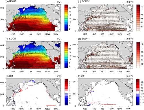
Figure 2 shows the annual mean sea surface temperature (SST) and velocity for 2011 in the North Pacific Ocean. The left and right columns show the distribution of SST and speed, respectively; the velocity vectors are superimposed on the maps. Figures 2a and 2b show the simulated result, and Figs 2c and 2d are derived from the Simple Ocean Data Assimilation (SODA version, 2.2.4; Carton, Chepurin, & Cao, 2000; Carton, Chepurin, Cao, & Giese, 2000). For SST, Figs 2a and 2c are generally similar. The difference is less than 1°C (Fig. 2e). By comparison, the simulated temperature is higher along the east coast of Japan, the Kuroshio Extension, and the west coast of North America and is lower around Bering Strait. Comparing the vectors for the velocity field in Fig. 2a with those in Fig. 2c, the large-scale circulations, including the North Pacific Gyre, Kuroshio, Kuroshio Extension, and the North Equatorial Current, have been satisfactorily simulated. For example, the North Equatorial Current flows from east to west, encounters the west boundary, and forms the Kuroshio. A branch of the Kuroshio intrudes into the South China Sea through Luzon Strait, but the main stream moves northwards. It branches into two parts after passing Taiwan. One intrudes into the ECS, becoming part of the Taiwan Warm Current. The Kuroshio flows out of the ECS through Tokara Strait, meeting the Oyashio Current off the coast of Japan near Fukushima and flows eastward into the North Pacific Ocean, which is known as the Kuroshio Extension. These currents are generally similar. But a discrepancy also exists (Fig. 2f). The speeds of the simulated and SODA surface flows are shown in Figs 2b and 2d. By comparison, the North Equatorial Current appears weaker in the simulation, and the Kuroshio and Kuroshio Extension are located a little northward. This problem, however, does not only occur here. As commented by Hasumi, Tatebe, Kawasaki, Kurogi, and Sakamoto (2010), “For a long-term simulation, this problem (the simulation of Kuroshio Extension) is almost unavoidable in most models nowadays. Even with high enough horizontal resolution to reproduce the Kuroshio separation from Japan’s coast, models tend to have problems in capturing its path and variability there.” Aside from this, the simulation of the large-scale circulations is, to an extent, satisfactory.

Fig. 2 Annual mean sea surface temperature (SST) and velocity for 2011 in the North Pacific Ocean. The left and right columns show the distributions of SST and speed, respectively; the velocity vectors are superimposed on the maps. (a) and (b) show the results from our simulation, and (c) and (d) are derived from SODA. (e) and (f) show the difference between model outputs and SODA data.

b East China Sea: SST and Currents

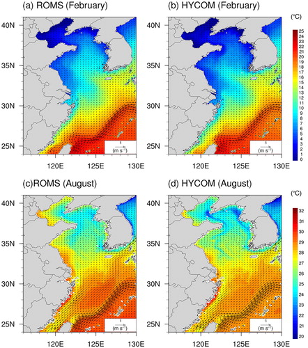
Figure 3 shows the monthly mean (2006–2011) SST and velocity in the ECS. Figure 3a shows the model simulation, and the right panel is from HYCOM. Generally, the two agree well in both summer and winter, except in August, when ROMS shows higher SSTs at the mouth of Bohai Sea. East Asia is a typical monsoon region, so the currents have strong seasonal variations. From Figs 3a and 3b, in winter (February), the coastal surface temperature is lower than in the open sea. West of Cheju Island, in the Yellow Sea, a warm tongue invades northwestward into the southern waters of Shandong Peninsula. Meanwhile, the Kuroshio, the Taiwan Warm Current, and the Tsushima Current are weak, and the Zhe-Min Coastal Current is southward. In summer (August; Figs 3c and 3d), the nearshore SST, as well as the Kuroshio and its branch, are strong, and the Zhe-Min Coastal Current flows northward. In the Yellow Sea, isolated cold patches are a conspicuous feature, which is especially clear off the tips of the peninsula. Our simulation captured all these features.

Fig. 3 ECS SST (shaded) and velocity (vectors) in winter and summer. (a) ROMS outputs, February; (b) HYCOM result, February; (c) ROMS outputs, August; and (d) HYCOM result, August.

c Surface ¹³⁷Cs Concentration

Table 4 shows the simulated results at the observation stations with (Run 2) and without (Run 1) assimilating the ¹³⁷Cs background radioactive concentration in the North Pacific; also shown are the measured concentrations. Considering that in our model the radionuclides are all released at the same time on 1 April 2011 rather than being released continuously as actually happened, the simulated concentration near the origin of the leak may not agree with observations; we thus exclude these stations (i.e., the stations in the area between 35°–45°N and 135°–150°E). This means that throughout the North Pacific Ocean 124 stations in total are available for validation from June 2011 to September 2012; these stations are indicated in Fig. 1a. As shown, there are many regions where the concentration of ¹³⁷Cs is zero in Run 1. In contrast, in Run 2, the concentrations are close to the observations. As another issue, concentration may vary dramatically in a single day (e.g., 21 January 2012 in Table 4). By comparing the observations from IAEA with Run 1 and Run 2, the average relative difference between Run 1 and the observations is 103.06%. In contrast, the Run 2 difference is only 18.79%. The average relative difference varies by region: it is 12.82% in the northeast Pacific, 23.39% in the central North Pacific, and 18.88% in the northwest Pacific. Considering that the average relative interdiurnal variation of the observations can be as high as 20.69%, Run 2 successfully reproduced the observed concentrations. That is to say, the simulation was significantly improved by taking into account the background ¹³⁷Cs concentration.

Table 4. Observations and the simulation output around ST-1 in 2012.

Date	Latitude (°N)	Longitude (°E)	Observation (Bq m^−3)	Simulation (Bq m^−3)
20 July 2012	36.005	155.01	1.3	1.5029
20 July 2012	38.010	155.08	1.8	1.4704
28 September 2012	44.575	156.08	2.2	1.6281
10 July 2012	44.000	155.01	3.0	2.0234
20 July 2012	37.010	155.01	1.1	1.5122
20 July 2012	36.462	155.06	1.1	1.5141
10 July 2012	43.012	155.01	2.8	1.4121
2 March 2012	37.500	161.82	9.4	4.9418
20 July 2012	35.002	155.01	3.6	1.4819
20 July 2012	40.002	155.01	3.6	1.4143
20 July 2012	40.512	155.01	6.5	1.9625
10 July 2012	40.997	155.06	8.0	4.6775
20 July 2012	39.505	155.05	5.5	1.4605
10 July 2012	42.530	155.10	6.5	1.5892
31 May 2012	38.500	160.00	9.3	5.1883

Aside from the magnitude, the simulated flow paths of the surface ¹³⁷Cs (Fig. 4) agree with previous studies (Behrens et al., 2012; Kawamura, Kobayashi, Furuno, Usui, & Kamachi, 2014; Nakano & Povinec, 2012; Povinec et al., 2013; Wang et al., 2012). Generally, the radionuclides followed the main stream of the Kuroshio Extension and arrived at the west coast of North America in the summer in 2014. Then some of the material moved northward along the coastline toward Bering Strait; some gathered off California and slowly spread southward; and some part flowed back to the western Pacific around 30°N, impacting the east coast of the Philippines in April 2014.

Fig. 4 Simulated surface distribution of ¹³⁷Cs in the North Pacific.

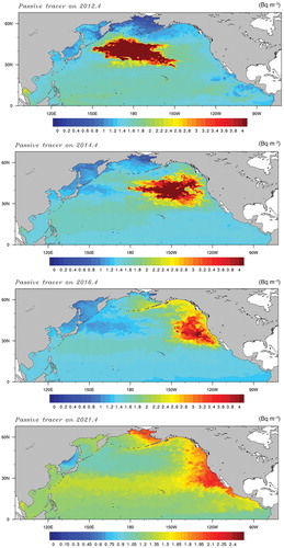
We also compared the horizontal and vertical distributions (Fig. 5) with previous studies, such as Nakano and Povinec’s (2012). Nakano and Provinec gave an annual mean vertical distribution of ¹³⁷Cs in 2012, 2014, 2016, and 2021 at Stations ST-1 (160°E, 40°N) east of Japan, ST-2 (175°W, 35°N) in the central North Pacific, ST-3 (125°W, 25°N) west of the United States, and ST-4 (130°E, 20°N) east of the Philippines. ST-1 is right on the Kuroshio Extension. In 2012, the averaged concentration of the surface layer was 20 Bq m⁻³ (Nakano & Povinec, 2012), which is much higher than that observed (4.05 Bq m⁻³ around ST-1 (155°–165°E, 35°–45°N) in 2012 (15 sites, see Table 4)). In our simulation, the maximum value appears at 140 m depth (3.31 Bq m⁻³), and the surface value is 2.91 Bq m⁻³, much closer to the observations. At the other three sites, according to Nakano and Provinec’s estimation, the averaged surface concentrations in 2012 were approximately zero, which is obviously not the case. ST-2 is located in the central North Pacific (185°W, 35°N), where Nakano and Provinec’s gives a maximum of 5 Bq m⁻³ in 2014. The observations show that the mean value at the surface around ST-2 (175°E–175°W, 25°–45°N) is 1.88 Bq m⁻³. The average concentration in our simulation over the observation sites is 2.56 Bq m⁻³ (four stations, see Table 5), and the averaged concentration in 2012 at ST-2 was 3.59 Bq m⁻³, and the maximum (3.77 Bq m⁻³) appears at a depth of 50 m. The ST-3 station is near the west coast of the United States. Around this site, there was only one observation with a concentration of 1.60 Bq m⁻³, where our simulated concentration was 1.69 Bq m⁻³ for the same time. The maximum annual average concentration appears in 2016 in our simulation, while in Nakano and Provinec’s, no significant concentration appears until 2021. There are no observational data around ST-4. Our model shows that the surface concentration is about 1.3 Bq m⁻³ (in 2021) to 1.6 Bq m⁻³ (in 2014), and reaches its maximum of 1.77 Bq m⁻³ around 140 m depth.

Fig. 5 Vertical profiles of ¹³⁷Cs at specific Pacific stations in our simulation.

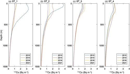
Table 5. Observations and the simulation output around ST-2 in 2012.

Date	Latitude (°N)	Longitude (°E)	Observation (Bq m^−3)	Simulation (Bq m^−3)
1 February 2012	33.050	204.72	1.6	1.7778
1 February 2012	27.840	189.10	2.1	1.8100
2 March 2012	33.420	196.11	2.1	3.1536
1 February 2012	32.980	197.06	1.7	3.5128

4. Impact on the East China coast

a ¹³⁷Cs Flux

In order to trace the origins of the ¹³⁷Cs along the ECS, we calculated the ¹³⁷Cs fluxes across the six waterways that connect the northwest Pacific with the ECS. These waterways are the Taiwan Strait, Tokara Strait, Tsushima Strait, and the channels between Taiwan and Yonaguni, Ishigaki and Naha, and Naha and Amami. Figure 6 presents the time series of the fluxes from April 2011 to December 2025 across these waterways. The time-averaged fluxes are tabulated in Table 7, with a negative sign signifying the outward direction. From Fig. 6, Taiwan Strait (Fig. 6a) and the Taiwan–Yonaguni channel (Fig. 6b) are the main waterways that introduce the pollutants. The flux through Taiwan Strait shows a significant seasonal change, which is high in summer and low in winter. East of Taiwan, the flux increases rapidly before 2013, followed by a decrease until early 2014, reaching its peak in 2017 then declining gradually. The influx of ¹³⁷Cs east of Taiwan is, on average, 3.70 × 10⁷ Bq s⁻¹, which is an order of magnitude lager than that through Taiwan Strait (2.81 × 10⁶ Bq s⁻¹).

Fig. 6 (a)–(f) Time series of the ¹³⁷Cs fluxes across the six waterways indicated in Fig. 1b (10⁶ Bq s⁻¹). Positive values indicate fluxes into the ECS; black lines are the moving averages with a window of 6 months. In (a) the red line (moving average in green) indicates the difference between the fluxes across the two sections B and G in Fig. 1b. (b) The red curve (moving average in green) is the flux across section G. (g) Total accumulation of nuclear pollutants in ECS (PBq). In all the panels, the April–September periods are shaded in yellow.

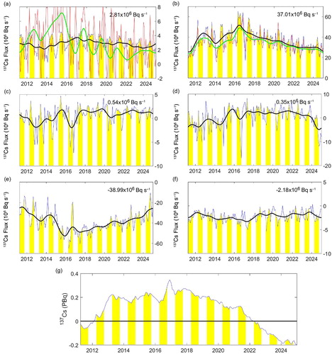
Table 7. Inflow flux through the six sections averaged over the period April 2011–December 2025. Negative values indicate outflow fluxes.

Section	Inflow Flux (10^6 Bq s^−1)	Section	Inflow Flux (10^6 Bq s^−1)
Taiwan Strait	2.81	East of Taiwan	37.01
Ishigaki to Naha	0.54	Naha to Amami	0.35
Tokara Strait	−38.99	Tsushima Strait	−2.18

The section from Ishigaki to Naha (Fig. 6c) and that from Naha to Amami Islands (Fig. 6d) are roughly parallel to the Kuroshio axis. They are also the main exchange waterways for the ECS and northwest Pacific, and the water depth is 1500 m. There is an exchange of water masses with a high ¹³⁷Cs concentration between the northwest Pacific and the ECS through the waterways. But because of the alignment, which is parallel to the Kuroshio path, the average fluxes in both waterways are orders of magnitude smaller (5.42 × 10⁵ Bq s⁻¹ and 0.52 × 10⁵ Bq s⁻¹, respectively) than those east of Taiwan and through Tokara Strait.

The ¹³⁷Cs is transported out of the ECS through Tokara Strait (Fig. 6e) and Tsushima Strait (Fig. 6f). The flux through the latter is 2.18 × 10⁶ Bq s⁻¹ and that through the former is as high as 3.90 × 10⁷ Bq s⁻¹. The outfluxes at the two straits are weak in winter and strong in summer, in accordance with the seasonal variation of the Kuroshio.

Figure 6g shows the cumulative sum of the ¹³⁷Cs through the six waterways of the ECS from April 2011 to December 2025. Before 2012, the sum is below zero, which means that the main part of ¹³⁷Cs in the ocean had not arrived in the ECS. After that, the sum gradually increases and reaches its peak in 2018 (0.13 PBq). One decade after the accident, the sum is again below zero. That is to say, it takes about 10 years for the ¹³⁷Cs concentration to return to its original level in the ECS.

b Nearshore Distribution and Seasonal Variability

Figure 7a shows that, after the accident, the surface ¹³⁷Cs concentration in the ECS peaks between 1.3 and 1.8 Bq m⁻³, depending on the location. It is high to the southeast of the ECS and decreases northwestward. The maximum is attained three years after the Fukushima accident along the Ryukyu Islands from Taiwan to Tokara Strait. On the whole, the concentration in the ECS reaches its peak in 2014, except near the coast of Zhejiang, where the peak appears in 2015. The simulation in the Yellow Sea is quite complex. The maximum concentration is about 1.4–1.5 Bq m⁻³, but it appears at different times for different regions. East of Lianyun Gang, it appears in 2018; from Subei Shoal to Cheju Island, it appears in 2014–2015; but from South Korea to Shandong Peninsula, the maximum is attained in 2016. The concentrations in the Bohai Sea and northern Yellow Sea and around Shandong Peninsula are no higher than before the accident.

Fig. 7 (a) Distribution of the simulated maximum surface ¹³⁷Cs concentration (lines, Bq m⁻³) and the year when it was attained (see colour bar). (b) Distribution of the maximum monthly mean ¹³⁷Cs radioactive concentration (lines, Bq m⁻³) and the months when the maximum was attained (shaded). The monthly mean is taken over the same months from 2014 to 2019. (c) Hovmöller diagram of ¹³⁷Cs concentration (shaded, Bq m⁻³) between 25°N and 37°N (green line in Fig. 1b) along the East China coast from 2011 to 2022.

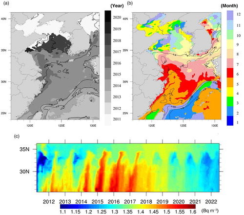
Generally speaking, the East China coast is most severely affected from 2014 to 2018. In particular, a relatively high concentration area (exceeding 1.45 Bq m⁻³) occurs on the eastern side of the Subei Bank. From the Hovmöller diagram (Fig. 7c), the maximum values occur around northern Taiwan Strait in winter between 25°N and 37°N along the East China coast (as shown in Fig. 1b) and spread northward until they reach Subei Bank in summer every year before 2019. In the Kuroshio region, the concentration is high and so is the concentration gradient. Following the Kuroshio to 35°N, the concentration is high from May to July. Along the Subei coast, the concentration peaks from August to November, while at the centre of the Yellow Sea, it reaches its maximum during September to November. For the rest of the region, such as the Bohai Sea and the northern Yellow Sea, the maximum appears in winter or early spring. All these suggest that the surface ¹³⁷Cs concentration has a strong seasonal variability.

As Fig. 7a shows, the peak ¹³⁷Cs in the ECS appears during the 2014–2019 period. Figure 6 displays the seasonal surface distribution of the ¹³⁷Cs concentration during this period. Generally speaking, the concentration decreases gradually from the southeast (1.6 Bq m⁻³) to the northwest (1.3 Bq m⁻³). From Fig. 7b, the maximum values around the Kuroshio occur in winter, while in the southern ECS the maximum occurs in late spring to summer. Lie and Cho (2002) point out that they occur in different water masses. From Fig. 6b, the rates of ¹³⁷Cs flux moving along the continental shelf (green line) is similar to that east of Taiwan but is lower than the latter, implying that the high concentration water masses move mainly along the continental shelf from Taiwan toward Tokara Strait. The remainder of the concentration affecting the Chinese coast through the Kuroshio Branch Current (the green line in Fig. 6a) contributes almost the same amount as that from Taiwan Strait (the black line in Fig. 6a). As shown in Fig 8, they flow northward along Fujian, Zhejiang (Fig. 8a), and Jiangsu (Fig. 8b), and then travel northeastward, finally flowing into the Japan Sea through Tsushima Strait (Figs 8c and 8d). During the process, the remnants mostly stay along the Jiangsu coast, giving a high ¹³⁷Cs concentration there in summer (Fig. 8c).

Fig. 8 Distributions of monthly mean surface ¹³⁷Cs concentration in the ECS from 2014 to 2019 for (a) January, (b) April, (c) July, and (d) October.

5 Conclusions

An earthquake of magnitude 9.0 occurred in the Pacific Ocean with a subsequent tsunami on 11 March 2011, severely damaging the Fukushima Dai-ichi Nuclear Power Plant and causing a nuclear leak. In this study, a two-domain, one-way nesting ROMS model was adopted to investigate the potential impact of the disaster on the East China coast. This model takes into account the background ¹³⁷Cs concentration and assimilates observations. It has been validated with available model results and observations.

Based on the prediction, we found that the accumulated ¹³⁷Cs in the ECS reaches its peak in 2018 and returns to its pre-accident level before 2021. Taiwan Strait and the channel east of Taiwan are the main waterways through which the pollutants flow into the ECS, and Tokara Strait and Tsushima Strait are the outlet waterways. The concentration has seasonal variability; usually winter is the season when the pollution is most severe. The maximum concentration along the East China coast is 1.3–1.8 Bq m⁻³. A conspicuous feature is the existence of a high around Subei Bank. The times that the maxima are attained vary from 2014 to 2018 depending on the latitude. Generally, the higher the latitude, the later the maximum is attained.

In summary, the radionuclides from the Fukushima nuclear leak have reached the ECS, though the concentration is still far below the safety threshold. The radionuclides come mainly from Taiwan Strait and the waterway east of Taiwan. The accumulated radionuclides are not homogeneously distributed; there are hotspots, such as the Subei Bank, where the concentration attains its maximum. These discoveries will be helpful for developing policy for rapid response to such disasters.

It should be mentioned that, until recently, the release of ¹³⁷Cs was still occurring, with the amount of the release unknown (Durović et al., 2016). That is to say, the impact of the nuclear leak on the ECS may have been underestimated in our computation. The nearshore pollution, in particular, could be more severe. This, among other issues, will be left to future studies.

Acknowledgements

We are grateful to IAEA for the ¹³⁷Cs observations, to OSU for the tidal constituent data, to NGDC for the ETOPO1 data, to the National Oceanographic Partnership Program (NOPP) for the HYCOM data, to the National Aeronautics and Space Administration for the SODA data, the reanalysis data, and the prediction data. Yineng Rong thanks Xiaochun Wang, Yuanbing Zhao, Yang Yang, and Minghai Huang for valuable discussions.

Disclosure statement

No potential conflict of interest was reported by the authors.

Additional information

Funding

This study was supported by the Jiangsu Provincial Government through the 2015 Jiangsu Program for Innovation Research and Entrepreneurship Groups and through the Jiangsu Chair Professorship to XSL, the National Science Foundation of China [grant number 41276032], and the National Program on Global Change and Air–Sea Interaction.

References

- Aoyama, M., Uematsu, M., Tsumune, D., & Hamajima, Y. (2013). Surface pathway of radioactive plume of TEPCO Fukushima npp1 released 134Cs and 137Cs. Biogeosciences, 10(5), 3067–3078. doi: 10.5194/bg-10-3067-2013
- Behrens, E., Schwarzkopf, F. U., Lübbecke, J. F., & Böning, C. W. (2012). Model simulations on the long-term dispersal of 137Cs released into the Pacific Ocean off Fukushima. Environmental Research Letters, 7(3), 34004–34013. doi: 10.1088/1748-9326/7/3/034004
- Bois, P. B. D., Laguionie, P., Boust, D., Korsakissok, I., Didier, D., & Fiévet, B. (2012). Estimation of marine source-term following Fukushima Dai-ichi accident. Journal of Environmental Radioactivity, 114(12), 2–9. doi: 10.1016/j.jenvrad.2011.11.015
- Buesseler, K., Aoyama, M., & Fukasawa, M. (2011). Impacts of the Fukushima nuclear power plants on marine radioactivity. Environmental Science & Technology, 45(23), 9931–9935. doi: 10.1021/es202816c
- Carton, J. A., Chepurin, G., & Cao, X. (2000). A simple ocean data assimilation analysis of the global upper ocean 1950–95. Part II: Results. Journal of Physical Oceanography, 30(2), 311–326. doi:10.1175/1520-0485(2000)030%3C0311:ASODAA%3E2.0.CO;2 doi: 10.1175/1520-0485(2000)030<0311:ASODAA>2.0.CO;2
- Carton, J. A., Chepurin, G., Cao, X., & Giese, B. (2000). A simple ocean data assimilation analysis of the global upper ocean 1950–95. Part I: Methodology. Journal of Physical Oceanography, 30(2), 294–309. doi:10.1175/1520-0485(2000)030%3C0294:ASODAA%3E2.0.CO;2 doi: 10.1175/1520-0485(2000)030<0294:ASODAA>2.0.CO;2
- Delworth, T. L., Rosati, A., Anderson, W., Adcroft, A. J., Balaji, V., Benson, R., … Zhang, R. (2012). Simulated climate and climate change in the GFDL CM2.5 high-resolution coupled climate model. Journal of Climate, 25(8), 2755–2781. doi: 10.1175/JCLI-D-11-00316.1
- Durović, B., Radjen, S., Radenković, M., Dragović, T., Tatomirović, Ž, Ivanković, N., … Dugonjić, S. (2016). Chernobyl and Fukushima nuclear accidents: What have we learned and what have we done? Vojnosanitetski pregled, 73(5), 484–490. doi: 10.2298/VSP160317061D
- Egbert, G. D., Bennett, A. F., & Foreman, M. G. G. (1994). TOPEX/Poseidon tides estimated using a global inverse model. Journal of Geophysical Research, 99(C12), 24821–24852. doi: 10.1029/94JC01894
- Egbert, G. D., & Erofeeva, S. Y. (2002). Efficient inverse modeling of barotropic ocean tides. Journal of Atmospheric and Oceanic Technology, 19(2), 183–204. doi:10.1175/1520-0426(2002)019%3C0183:EIMOBO%3E2.0.CO;2 doi: 10.1175/1520-0426(2002)019<0183:EIMOBO>2.0.CO;2
- Hasumi, H., Tatebe, H., Kawasaki, T., Kurogi, M., & Sakamoto, T. T. (2010). Progress of North Pacific modeling over the past decade. Deep Sea Research Part II: Topical Studies in Oceanography, 57(13–14), 1188–1200. doi: 10.1016/j.dsr2.2009.12.008
- He, Y. C., Gao, Y. Q., Wang, H. J., Ola, J. M., & Yu, L. (2012). 2011年日本福岛核电站泄露在海洋中的传输 [Transport of nuclear leakage from Fukushima nuclear power plant in the North Pacific]. Acta Oceanologica Sinica, 34(4), 12–20.
- Hirose, K. (2012). 2011 Fukushima Dai-ichi nuclear power plant accident: Summary of regional radioactive deposition monitoring results. Journal of Environmental Radioactivity, 111(5), 13–17. doi: 10.1016/j.jenvrad.2011.09.003
- Kalnay, E., Kanamitsu, M., Kistler, R., Collins, W., Deaven, D., Gandin, L., … Wang, J. (1996). The NCEP/NCAR 40-year reanalysis project. Bulletin of the American Meteorological Society, 77(3), 437–471. doi: 10.1175/1520-0477(1996)077<0437:TNYRP>2.0.CO;2
- Kawamura, H., Kobayashi, T., Furuno, A., In, T., Ishikawa, Y., Nakayama, T., … Awaji, T. (2011). Preliminary numerical experiments on oceanic dispersion of 131I and 137Cs discharged into the ocean because of the Fukushima Daiichi nuclear power plant disaster. Journal of Nuclear Science and Technology, 48(11), 1349–1356. doi: 10.1080/18811248.2011.9711826
- Kawamura, H., Kobayashi, T., Furuno, A., Usui, N., & Kamachi, M. (2014). Numerical simulation on the long-term variation of radioactive cesium concentration in the North Pacific due to the Fukushima disaster. Journal of Environmental Radioactivity, 136, 64–75. doi: 10.1016/j.jenvrad.2014.05.005
- Lai, Z., Chen, C., Beardsley, R., & Lin, H. (2013). Initial spread of 137Cs over the shelf of Japan: A study using the high-resolution global-coastal nesting ocean model. Biogeosciences Discussions, 10(2), 1929–1955. doi: 10.5194/bgd-10-1929-2013
- Leon, J. D., Jaffe, D. A., Kaspar, J., Knecht, A., Miller, M. L., Robertson, R. G. H., & Schubert, A. G. (2011). Arrival time and magnitude of airborne fission products from the Fukushima, Japan, reactor incident as measured in Seattle, WA, USA. Journal of Environmental Radioactivity, 102(11), 1032–1038. doi: 10.1016/j.jenvrad.2011.06.005
- Liang, X. S., & Robinson, A. R. (2013). Absolute and convective instabilities and their roles in the forecasting of large frontal meanderings. Journal of Geophysical Research: Oceans, 118(10), 5686–5702. doi: 10.1002/jgrc.20406
- Lie, H. J., & Cho, C. H. (2002). Recent advances in understanding the circulation and hydrography of the East China Sea. Fisheries Oceanography, 11(6), 318–328. doi: 10.1046/j.1365-2419.2002.00215.x
- Masamichi, C., Hiromasa, N., Haruyasu, N., Hiroaki, T., Genki, K., & Hiromi, Y. (2011). Preliminary estimation of release amounts of 13Li and 137Cs accidentally discharged from the Fukushima Daiichi nuclear power plant into the atmosphere. Journal of Nuclear Science & Technology, 48(7), 1129–1134. doi: 10.1080/18811248.2011.9711799
- Mason, E., Molemaker, J., Shchepetkin, A. F., Colas, F., Mcwilliams, J. C., & Sangrà, P. (2010). Procedures for offline grid nesting in regional ocean models. Ocean Modelling, 35(1-2), 1–15. doi: 10.1016/j.ocemod.2010.05.007
- MEXT (Ministry of Education, Culture, Sports, Science and Technology). (2012). 平成24年版科学技術白書 [Science and Technology White Paper (2012 Edition)]. Retrieved from http://www.mext.go.jp/b_menu/hakusho/html/hpaa201201/detail/1322695.htm
- Nakano, M., & Povinec, P. P. (2012). Long-term simulations of the 137Cs dispersion from the Fukushima accident in the world ocean. Journal of Environmental Radioactivity, 111(111), 109–115. doi: 10.1016/j.jenvrad.2011.12.001
- NGDC. (2015). ETOPO1 Global Relief Model. Retrieved from http://www.ngdc.noaa.gov/mgg/global/global.html
- Povinec, P., Chudý, M., Sýkora, I., Szarka, J., Pikna, M., & Holý, K. (1988). Aerosol radioactivity monitoring in Bratislava following the Chernobyl accident. Journal of Radioanalytical and Nuclear Chemistry Letters, 126(6), 467–478. doi: 10.1007/BF02164550
- Povinec, P. P., Gera, M., Holý, K., Hirose, K., Lujaniené, G., Nakano, M., … Gažák, M. (2013). Dispersion of Fukushima radionuclides in the global atmosphere and the ocean. Applied Radiation and Isotopes, 81(2), 383–392. doi: 10.1016/j.apradiso.2013.03.058
- Rong, Y. N., Xu, R., Liang, X. S., & Zhao, Y. B. (2016). 福岛核泄漏事件对中国海污染的研究 [A study of the possible radioactive contamination in the China Seas from the Fukushima nuclear disaster]. Acta Scientiae Circumstantiae, 36(9), 3146–3159. doi: 10.13671/j.hjkxxb.2016.0086
- Saenko, V., Ivanov, V., Tsyb, A., Bogdanova, T., Tronko, M., Demidchik, Y., & Yamashita, S. (2011). The Chernobyl accident and its consequences. Clinical Oncology, 23(4), 234–243. doi: 10.1016/j.clon.2011.01.502
- Takemura, T., Nakamura, H., Takigawa, M., Kondo, H., Satomura, T., Miyasaka, T., & Nakajima, T. (2011). A numerical simulation of global transport of atmospheric particles emitted from the Fukushima Daiichi nuclear power plant. Scientific Online Letters on the Atmosphere Sola, 7(1), 101–104. doi: 10.2151/sola.2011-026
- Tohoku Earthquake Tsunami Joint Survey Group. (2011). Nationwide field survey of the 2011 off the Pacific coast of Tohoku earthquake tsunami. Journal of Japan Society of Civil Engineers, Ser. B2 (Coastal Engineering), 67(1), 63–66. doi: 10.2208/kaigan.67.63
- Tsumune, D., Aoyama, M., & Hirose, K. (2003). Behavior of 137Cs concentrations in the North Pacific in an ocean general circulation model. Journal of Geophysical Research, 108(C8), 57. doi: 10.1029/2002JC001434
- Tsumune, D., Tsubono, T., Aoyama, M., & Hirose, K. (2012). Distribution of oceanic 137Cs from the Fukushima Dai-ichi nuclear power plant simulated numerically by a regional ocean model. Journal of Environmental Radioactivity, 111, 100–108. doi: 10.1016/j.jenvrad.2011.10.007
- Wang, H., Wang, Z. Y., Zhu, X. M., Wang, D. K., & Liu, G. M. (2012). Numerical study and prediction of nuclear contaminant transport from Fukushima Daiichi nuclear power plant in the North Pacific Ocean. Chinese Science Bulletin, 57(26), 3518–3524. doi: 10.1007/s11434-012-5171-6
- Wu, J. W., Zhou, K. B., & Dai, M. H. (2013). Impacts of the Fukushima nuclear accident on the China Seas: Evaluation based on anthropogenic radionuclide 137Cs. Chinese Science Bulletin, 58(4-5), 552–558. doi: 10.1007/s11434-012-5426-2
- Zhao, C., Qiao, F., Wang, G., Shu, Q., & Xia, C. (2015). 历次核试验进入海洋的137Cs对中国近海影响的模拟研究 [Simulation of the influence of 137Cs from nuclear experiments on China Seas]. Acta Oceanologica Sinica, 37(3), 15–24. doi: 10.369/j/issn.0253-4193.2015.03.002
- Zhao, C., Qiao, F. L., Wang, G. S., Xia, C. S., & Jung, K. T. (2014). 福岛核事故泄漏进入海洋的 137Cs 对中国近海影响的模拟与预测 [Simulation and prediction of 137Cs from the Fukushima accident in the China Seas]. Chinese Science Bulletin (Chinese Version), 59(34), 3416–3423. doi: 10.1360/N972014-00012