Response of the Tropical Indian Ocean to Greenhouse Gases and Aerosol Forcing in the GFDL CM3 Coupled Climate Model

ABSTRACT

The response of the tropical Indian Ocean (TIO) to greenhouse gases (GHGs) and aerosols are investigated based on historical single-forcing and all-forcing simulations using the Geophysical Fluid Dynamics Laboratory Climate Model, version 3 (GFDL CM3). Results reveal a positive Indian Ocean Dipole (pIOD)-like pattern in GHG forcing but a negative Indian Ocean Dipole (nIOD)-like pattern in aerosol forcing. The GHG-induced pIOD-like pattern features less (more) sea surface temperature (SST) warming over the southeastern (western) TIO, accompanied by equatorial easterly anomalies, as well as a shallower thermocline off Sumatra. The aerosol-induced nIOD-like pattern displays the reverse features, characterized by less (more) SST cooling over the southeastern (western) TIO, anomalous equatorial westerlies, and a deeper thermocline off Sumatra. Although the aerosol-induced pattern appears to resemble a reversal of the GHG-induced pattern, there is a strong asymmetry in the SST changes over the southeastern TIO, where the cooling responding to aerosol forcing exceeds the warming in response to GHG forcing, and a negative SST residual is thus produced. A mixed-layer heat budget analysis suggests that the negative SST residual results mainly from asymmetric responses of shortwave radiation, zonal advection, and diffusion to GHGs and aerosols. For comparison, the formation processes for the negative SST skewness over the southeastern TIO between the internal pIOD and nIOD are also discussed.

Résumé

[Traduit par la rédaction] Nous étudions la réaction de l’océan Indien tropical aux gaz à effet de serre (GES) et aux aérosols sur la base de simulations, à forçage unique ou à forçages multiples, provenant de la version 3 du modèle climatique du Geophysical Fluid Dynamics Laboratory (GFDL CM3). Les résultats révèlent une configuration ressemblant à un dipôle de l’océan Indien positif (pIOD) pour les GES, mais à un dipôle de l’océan Indien négatif (nIOD) pour les aérosols. Cette espèce de dipôle positif que produisent les GES s’accompagne d’un réchauffement de la température de surface de la mer (SST) moins (plus) important dans le sud-est (l’ouest) de l’océan Indien tropical, et ce, en plus de vents d’est équatoriaux anormaux et d’une thermocline peu profonde au large de Sumatra. En revanche, l’espèce de dipôle négatif que produisent les aérosols présente des caractéristiques inverses. Le refroidissement de la température de surface de la mer s’avère moins (plus) important dans le sud-est (l’ouest) de l’océan Indien tropical, et ce, en plus de vents d’ouest équatoriaux anormaux et d’une thermocline profonde au large de Sumatra. Bien que la configuration due aux aérosols semble être l’inverse de la configuration émanant des GES, il existe une forte asymétrie dans l’évolution des SST dans le sud-est de l’océan Indien tropical, où le refroidissement correspondant aux aérosols dépasse le réchauffement dû aux GES, ainsi des SST résiduelles négatives dominent. L’analyse du bilan thermique de la couche de mélange laisse penser que les SST résiduelles négatives proviennent principalement de la réaction asymétrique du rayonnement d’ondes courtes, de l’advection zonale et de la diffusion que produisent les GES et les aérosols. Nous présentons aussi, aux fins de comparaison, le processus de formation du biais négatif des SST dans le sud-est de l’océan Indien tropical, entre les dipôles positif et négatif internes de l’océan Indien.

Keywords:

• Indian Ocean Dipole
• greenhouse gases
• aerosols
• IOD skewness
• SST residual

1 Introduction

The Indian Ocean Dipole (IOD) is an ocean–atmosphere coupled mode over the tropical Indian Ocean (TIO), characterized by an anomalous west–east sea surface temperature (SST) gradient accompanying wind and precipitation anomalies (Saji, Goswami, Vinayachandran, & Yamagata, 1999). The dipole events are seasonally phase locked: significant anomalies first appear in May–June, intensify in the following months, and mature in October, followed by a rapid demise. Among a range of feedbacks associated with IOD events, the positive Bjerknes feedback (Bjerknes, 1969) is believed to be the leading mechanism for the production of the cooling anomaly over the southeastern TIO (ETIO) during the northern fall. Li, Wang, Chang, and Zhang (2003) suggested that seasonally dependent thermodynamic air–sea feedback mechanisms could, to a large extent, explain the rapid development of the IOD during the northern summer and its mature phase in autumn. Additionally, the indirect effect of El Niño on the Indian Ocean through the anomalous monsoon may also play an integral role in the phase locking.

There are two phases of the dipole mode, similar to the El Niño and La Niña phases of El Niño–Southern Oscillation events. During a positive IOD (pIOD) event, SST is cooler than normal in the ETIO but warmer than usual in the western TIO (WTIO), with anomalous easterlies blowing around the equatorial central and eastern Indian Ocean. During a negative IOD (nIOD) event, the above patterns are reversed. Previous studies have found that a notable amplitude asymmetry in SST anomalies (SSTAs) exists between the positive and negative phases of IOD events, with the former being much larger in amplitude (Cai et al., 2013; Cai & Qiu, 2013; Cai, van Rensch, Cowan, & Hendon, 2012; Hong, Li, Ho, & Kug, 2008; Zheng, Xie, Vecchi, Liu, & Hafner, 2010). The negative SST skewness in the ETIO is the primary contributor to this asymmetry (Hong et al., 2008), with cold SSTAs during pIOD events being able to grow larger than warm SSTAs during nIOD events off Sumatra–Java (Cai et al., 2013), referred to as the negative SST skewness, hereafter. In terms of the cause of negative SST skewness, several possible physical mechanisms have been proposed, including non-linear ocean temperature advection (Hong et al., 2008; Ng, Cai, & Walsh, 2014), the asymmetric cloud-radiation-SST feedback (Hong et al., 2008; Hong & Li, 2010), and a non-linear thermocline–temperature feedback (Zheng et al., 2010).

Over the past century, emissions of anthropogenic aerosols and greenhouse gases (GHGs) have increased dramatically as a result of rapid industrialization (Wang, Xie, & Liu, 2016). Available observations and reanalysis shows that the occurrence of pIODs has increased in frequency since the 1950s (Cai, Cowan, & Sullivan, 2009b; Ihara, Kushnir, & Cane, 2008). The high frequency of pIOD events accounts for the recent austral winter and spring rainfall decline over southeastern Australia (Cai, Cowan, & Sullivan, 2009b), and the future climate will continue to raise the bushfire risk (Cai, Cowan, & Raupach, 2009a). In addition, climate models project that the frequency of extreme pIOD events will also increase significantly under global warming (Cai et al., 2014). On the other hand, climate models show that global warming induces a pIOD-like warming pattern over the TIO (e.g., Luo, Lu, Liu, & Wan, 2016; Zheng et al., 2013), featuring less SST warming over the ETIO, associated with easterly anomalies along the equator and shoaling of the thermocline over the ETIO. In stark contrast to GHGs, anthropogenic aerosols tend to impose negative radiative forcing to the coupling system.

Recent studies have explored the influence of GHGs and aerosols on the TIO (Cowan, Cai, Ng, & England, 2015; Dong & Zhou, 2014). Using 17 models from phase 5 of the Coupled Model Intercomparison Project (CMIP5), Dong and Zhou (2014) examined the roles of GHGs and aerosols in forming the pIOD-like warming pattern, with a focus on the linear relationship between the pIOD-like pattern and the surface easterly wind anomaly along the equator. They found that GHG forcing dominates the pIOD-like pattern, while aerosol forcing tends to induce an nIOD-like pattern, which acts to weaken the effect of GHGs. By analyzing 10 CMIP5 models, Cowan et al. (2015) found that aerosols enhance negative SST skewness over the ETIO more than GHGs because of the asymmetric SST–thermocline feedback.

In this paper, we analyze simulations with historical anthropogenic aerosol single forcing and GHG single forcing from the Geophysical Fluid Dynamics Laboratory Climate Model, version 3 (GFDL CM3) to examine the influence of GHGs and aerosols on the SST pattern over the TIO. Consistent with earlier conclusions (Cowan et al., 2015; Dong & Zhou, 2014), GHGs are found to induce a pIOD-like SST warming pattern, while aerosols act to produce an nIOD-like SST pattern. However, differing from previous studies, we also found that an asymmetry exists in the amplitude of SST changes responding to GHGs and aerosols, with most of the TIO displaying a positive SST residual except the ETIO, where the cooling responding to aerosol forcing surpasses the warming responding to GHG forcing, leading to a negative SST residual. Furthermore, in this study, a mixed-layer heat budget analysis is used to help in understanding the physical mechanisms responsible for this ETIO negative SST residual, by comparing the origin of the ETIO SST skewness between internal pIOD and nIOD events.

The rest of this paper is structured as follows. Section 2 describes the model and data. Section 3 introduces the methods used for compositing the internal pIOD and nIOD events. Oceanic and atmospheric changes over the TIO under GHG forcing and aerosol forcing are presented in Section 4. Section 5 discusses the SST residual and IOD asymmetry, with a mixed-layer heat budget analysis conducted to help understand the difference in their formation processes. Section 6 presents a discussion on the changes in the Indonesian Throughflow (ITF) under GHG and aerosol forcing and its influence on ocean circulation over the ETIO. Section 7 summarizes our main findings.

2 Model and data

This study uses outputs from the newest version of GFDL CM3 from the National Oceanic and Atmospheric Administration (NOAA), which is a coupled general circulation model for the atmosphere, oceans, land, and sea ice (Donner et al., 2011). The elements of the ocean and sea-ice simulations are documented in Griffies et al. (2011), and the basic simulation characteristics of the atmospheric component are described in Donner et al. (2011). The atmospheric component of GFDL CM3 is the Atmospheric Model, version 3 (AM3), which uses a cubed-sphere implementation of a finite-volume dynamical core. Its horizontal resolution is approximately 200 km, and its vertical resolution ranges from approximately 70 m near the Earth's surface to 1 to 1.5 km near the tropopause and 3 to 4 km in much of the stratosphere. The ocean model component of CM3 is based on the Modular Ocean Model, version 4p1 (MOM4p1) code, with 1° × 1° horizontal resolution and the meridional resolution gradually increasing to 1/3° at the equator between 30°S and 30°N. It has 50 vertical levels each 10 m thick in the top 22 levels.

Following CMIP5 protocol (Taylor, Stouffer, & Meehl, 2012), the GFDL CM3 has performed a number of integrations, including an 800-year-long pre-industrial control run, a historical all-forcing run, as well as a few historical single-forcing simulations for 1860–2005. The 800-year-long control run consists of a 500-year-long constant radiative forcing in 1860 and a 300-year-long forcing of a smaller constant based on new solar irradiance measurements (Griffies et al., 2011). The historical all-forcing simulation is performed to replicate the climate change of 1860–2005 with all forcings being time-varying. The historical single-forcing simulations aim to estimate the contribution of an individual radiative forcing mechanism to recent climate change, with the GHGs or aerosols being the only time-varying forcing and the other forcing kept fixed at the pre-industrial level. Thereby, the relative contribution of GHG- or aerosol-induced radiative forcing to climate change can be evaluated through the comparison of historical all forcing with a single forcing.

In this paper, the 56-year-long (1950–2005) GHG-only, aerosol-only, and historical all-forcing simulations are used in the analysis. In order to suppress the internal variability from an individual simulation, we selected three members of each simulation and then obtained their ensemble means. Additionally, the control run is used as a reference for all three experiments, as well as to construct the pIOD and nIOD composites. Note that the monthly climatology is averaged over the 1950–2005 period for GHG-only, aerosol-only, and all-forcing simulations. The anomalies are the differences between the control run and the three-member ensemble mean or composites.

Before presenting the model results, we verified the model's ability to simulate the TIO by comparing the historical all-forcing simulation with a series of reanalysis products including temperature from the Simple Ocean Data Assimilation (SODA)-Parallel Ocean Program, version 2.24, SST data from the Hadley Centre Global Sea Ice and SST (HadISST1) reanalysis, and 10 m zonal wind from the European Centre for Medium-range Weather Forecasts (ECMWF) global atmospheric reanalysis (ERA-Interim), following the methods of Weller and Cai (2013), Cai and Cowan (2013), and Cai and Qiu (2013). The SST and wind, along with their seasonal evolutions, were simulated well by the historical all-forcing run of GFDL CM3; the east–west thermocline depth gradient was also simulated well (not shown).

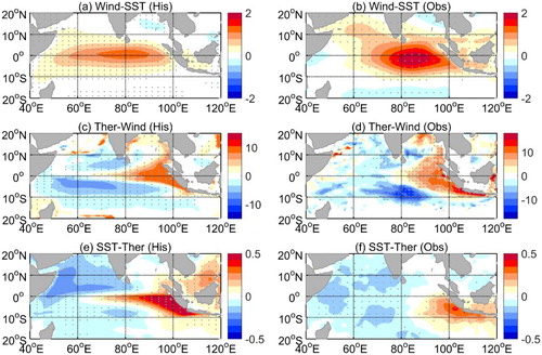
Figure 1 shows a model–observation comparison of the sensitivities of zonal winds to the ETIO SST (Figs 1a and 1b), thermocline depth to zonal winds over the central equatorial Indian Ocean (CEIO, 5°S–5°N, 80°–100°E; Figs 1c and 1d), and SST to ETIO thermocline depth (Figs 1e and 1f), which constitute the Bjerknes positive feedback loop and represent the strength of the Bjerknes feedback (Cai & Qiu, 2013; Cowan et al., 2015). It can be clearly seen that, in spite of some biases in the model, such as weaker sensitivity of both zonal winds to ETIO SST and thermocline depth to CEIO zonal winds and stronger sensitivity of SST to ETIO thermocline depth, the model is reliable for use in understanding ocean dynamics and air–sea interactions over the TIO.

Fig. 1 Sensitivity of 10 m zonal wind to ETIO SST (m s⁻¹) for the September–November period, calculated from (a) the GFDL CM3 historical all-forcing simulation for the 1950–2005 period and (b) the HadISST1 and ERA-Interim zonal winds both from 1979 to 2010. The sensitivity is obtained by multiplying the regression coefficient by one standard deviation of the value of the predictor, following the method of Weller and Cai (2013) and Cai and Cowan (2013). Sensitivity of thermocline depth to CEIO zonal winds (m) for the September–November period, calculated from (c) the GFDL CM3 historical all-forcing simulation for the 1950–2005 period and (d) the SODA temperature and ERA-Interim zonal winds both from 1979 to 2010. Sensitivity of SST to ETIO thermocline depth (°C) for the September–November period, calculated from (e) the GFDL CM3 historical all-forcing simulation for the 1950–2005 period, and (f) the HadISST1 and SODA temperature both from 1979 to 2010. Statistically significant correlations over the 95% confidence level are shown as grey dots.

3 Composites of pIOD and nIOD

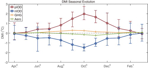
We construct the pIOD and nIOD composites following the procedure of Luo et al. (2016), who constructed the pIOD composite based on a warmer climate simulation with the Community Earth System Model from the National Center for Atmospheric Research (NCAR). To formulate a pIOD or nIOD composite without the influence of the anthropogenic aerosol- or GHG-induced radiative forcings, the pre-industrial control experiment is used to calculate the IOD index (DMI), which is defined as the difference in SSTAs between the WTIO (50°–70°E, 10°S–10°N) and the ETIO (90°–110°E, 10°S–equator) (Saji et al., 1999). In this analysis, 20 pIOD events and 14 nIOD events are identified during the 106-year control simulation based on the criterion that the September–November DMI exceeds one standard deviation (black bars in Fig. 2). Because the DMI time series is characterized by seasonal phase locking (Fig. 3), we divide the evolution of the pIOD and nIOD events into three distinct stages: (i) June–August of year zero as the development phase; (ii) September–November of year zero as the peak phase; and (iii) December of year zero to February of year one as the decay phase. Moreover, in order to facilitate the comparison of the internal IOD events and radiative forcings, we extract 12 months from April of year zero to March of year one as one “IOD year”.

Fig. 2 Time series of September–November IOD index from year 41 to 146 based on the pre-industrial control experiment data. The horizontal dashed lines at ±1.03°C (one standard deviation of DMI) are used as the threshold to define the IOD events; black bars indicate the 20 pIOD events and 14 nIOD events that are identified during the 106-year control simulation period.

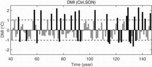
Fig. 3 Seasonal evolutions of the IOD index under the pIOD composite (red), nIOD composite (blue), GHG-only simulation (yellow), and aerosol-only simulation (green). Superscripts 0 and 1 in April, June, August, October, December, and February denote year 0 and year 1, respectively. The error bars represent the upper and lower limits of the composites.

4 Changes over the TIO under GHG and aerosol forcings

a Spatial Patterns during the Mature Season

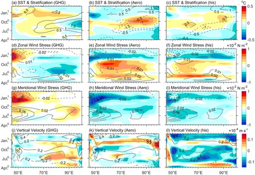
Figures 4 and 5 show various features under the GHG-only forcing (first column), aerosol-only forcing (second column), and historical all-forcing (last column) from September to November. Note that the basin means (averaged over 20°S–20°N in the Indian Ocean) of SSTAs have been removed in Figs 4a–4c, to facilitate the comparison of the GHG-only run, the aerosol-only run, and the all-forcing run. Thus, SST cooling (warming) in Fig. 4a (Fig. 4b) represents SST warming (cooling) that is less than the basin mean warming (cooling).

Fig. 4 The GHG-only (first column), aerosol-only (second column), and historical all-forcing-induced (last column) changes for the September–November period: (a), (b), and (c) SST (°C); (d), (e), and (f) wind stress (Pa) and its magnitude ( × 10⁻²Pa); (g), (h), and (i) sea surface zonal velocity (colour) and current fields (m s⁻¹) (vectors); (j), (k), and (l) vertical velocity (colour, 10⁻⁴ m s⁻¹) and stratification fields at a depth of 55 m (contours, 10⁻²°C m⁻¹). A positive vertical velocity indicates upwelling. Superimposed in (a), (b), and (c) are the climatological fields of the corresponding variables during boreal fall. SSTAs in (a), (b), and (c) are further normalized by removing the mean value of the field between 20°S and 20°N in the Indian Ocean.

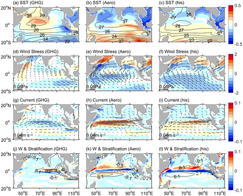
Fig. 5 The GHG-only (first column), aerosol-only (second column), and historical all-forcing-induced (last column) changes (shading, W m⁻²) and their corresponding climatological fields (contours, W m⁻²) for the September–November period: (a), (b), and (c) surface heat flux; (d), (e), and (f) latent heat flux; (g), (h), and (i) longwave radiation; (j), (k), and (l) shortwave radiation. A positive heat flux (downward) indicates warming of the ocean.

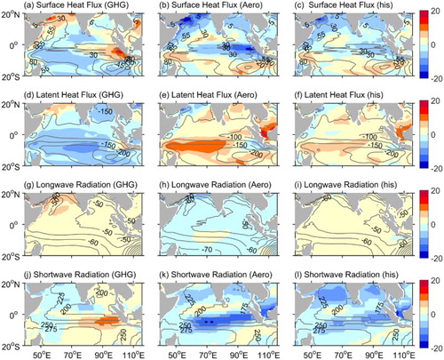
Under GHG forcing, the SSTAs display a clear pIOD-like pattern over the TIO, with reduced warming off the Sumatra–Java coast and enhanced warming in the WTIO (Fig. 4a). The SSTA dipole is accompanied by a surface equatorial easterly wind change (Fig. 4d), consistent with a slowdown of the Walker circulation under global warming (Cai et al., 2013). The weakened Walker circulation will be conductive to the surface and subsurface thermal structure change, especially over the ETIO. The thermocline is deep under normal conditions over the ETIO but is raised by the upwelling anomalies associated with the anomalous easterlies and equatorial westward currents (Fig. 4g). Another signature of the response in the ETIO region is a significant intensification of the upper-ocean stratification along the Sumatra–Java coast (contours in Fig. 4j). In the GHG run, the ETIO is characterized by heat uptake from the atmosphere, but over the WTIO heat is lost to the atmosphere (Fig. 5a), acting to damp the formation of the pIOD-like mode. The heat uptake is mainly attributed to the warming effect of shortwave radiation over the ETIO (Fig. 5j), while the heat loss results from the cooling effect of both shortwave radiation and latent heat flux over the WTIO (Fig. 5d). The shortwave radiation acts to warm (cool) the upper ocean over the ETIO (WTIO). This warming (cooling) effect is closely related to the decrease (increase) in cloudiness, which will reflect less (more) incoming solar radiation back into space, indicative of the possible role of cloud-radiation-SST feedback in regulating the coupling system over the TIO. Latent heat flux is a major cooling source for the TIO and crucial for SST pattern formation through wind-evaporation SST feedback and Newtonian damping (Xie et al., 2010). In addition, anomalous longwave radiation exerts a basin-wide warming effect on the TIO (Fig. 5g), resulting from the combined effects of water vapour, cloud cover, and SST (Wallace & Hobbs, 2006). The sign of the longwave radiation anomaly is mainly determined by two competing effects: following Stefan–Boltzman's law, a warmer ocean will emit more upward longwave radiation, while the increased water vapour and cloud cover tends to trap more longwave radiation and reflect it back to the sea surface (Liu, Luo, Lu, Garuba, & Wan, 2017). Under GHG forcing, more trapped infrared radiation than heat will escape from the ocean, thus producing a positive longwave radiation anomaly over the TIO. The sensible heat flux is not shown here because it is negligible compared with the other three components of the surface heat flux.

In stark contrast to what happens under GHG forcing, the mean climate conditions shift toward an nIOD-like state under aerosol forcing with features such as reduced cooling in the ETIO but enhanced cooling in the WTIO (Fig. 4b), equatorial westerly anomalies (Fig. 4e), deepening thermocline, and weakening stratification over the ETIO (contours in Fig. 4k). These qualitative similarities in spatial distribution reflect the fact that GHG-induced and aerosol-induced climate responses share key ocean–atmosphere feedbacks (Xie, Lu, & Xiang, 2013). On closer inspection of the response to GHG forcing versus aerosol forcing, many of the changes are not symmetric. For example, while GHG forcing induces weak southeasterlies over the central and eastern equatorial Indian Ocean, aerosol forcing induces strong northwesterlies over the central and western equatorial Indian Ocean. The asymmetric wind stress response produces an asymmetric response in surface currents (Figs 4g and 4h), with the eastward anomalies under aerosol forcing being larger than the westward anomalies under GHG forcing. In addition, the aerosol-induced heat flux response (Fig. 5b) differs significantly from that induced by GHG. In the aerosol run, the equatorial Indian Ocean features heat loss to the atmosphere. The heat loss results mainly from the cooling effect of shortwave radiation (Fig. 5k) as a result of reduced downward solar radiation in response to increased cloud cover and atmospheric aerosols. The cooling effect from longwave radiation in the aerosol run (Fig. 5h) is also in stark contrast to the warming effect in the GHG run. Aerosols can absorb, reflect, and scatter radiation in the atmosphere, resulting in reduced downward shortwave radiation (Fig. 5k). The cooler ocean induced by the reduction in downward shortwave radiation tends to emit less upward longwave radiation into the atmosphere. Meanwhile, aerosols also influence longwave radiation through aerosol–cloud interactions. In more detail, aerosol particles, such as sulphate, serve as cloud condensation nuclei or ice nuclei and interact with clouds to absorb longwave radiation and increase cloud albedo. As a result, less downward longwave radiation will reach the ocean. Furthermore, aerosols tend to increase the lifetime, thickness, and amount of cloud, as well as decrease precipitation efficiency, significantly reducing downward longwave radiation in the long-term (Boucher et al., 2013; Wang et al., 2016). The combination of the two influences of aerosols leads to negative longwave radiation and thus a cooling of the TIO. Moreover, in contrast to the cooling effect in the GHG run, latent heat flux plays a warming role over the central and western TIO in the aerosol run (Fig. 5e).

We also compare climate response patterns between single-forcing simulations and the historical run. On the one hand the sum of the changes from GHG and aerosol single-forcing runs are quite similar to the distribution patterns in the historical all-forcing run. On the other hand, compared with the GHG scenario, the patterns of aerosol-induced changes are more similar to the patterns in the historical run (Fig. 4a–4l), such as the anomalous westerlies, eastward currents and downwelling along the equator, the positive SSTA, and reduced stratification over the ETIO. This suggests that the aerosol effect exceeds the GHG effect over the TIO.

b Seasonal Evolution

For the GHG-induced seasonal evolution, anomalous SST cooling first arises off Sumatra in June–July (Fig. 6a), accompanied by anomalous southeasterly winds over the ETIO (Figs 6d and 6g). The anomalous winds further enhance the mean southeasterly trade winds that, in turn, intensify surface evaporation, coastal upwelling (Fig. 6j), westward current, as well as interrupt the normal heat supply from the west to the coast off Sumatra. Thereby, the anomalous intensified trade winds and sequence of changes further cool the ETIO in the following months, while the WTIO is warming due to the anomalous westward current, enhanced Ekman convergence, and downwelling. Zonal wind anomalies intensify together with the SST dipole along the equator. A dramatically rapid peak in these features occurs in September followed by a rapid decay. Under aerosol forcing, on the contrary, anomalous SST cooling occurs around the equator until July (Fig. 6b), accompanied by northwesterly anomalies (Figs 6e and 6h). In July–August, positive SSTAs appear in the central and western equatorial Indian Ocean followed by an eastward shift and reach a peak in October. While the maximum warm anomalies are accompanied by weak westerly anomalies in the east, weak warm anomalies, along with maximum westerly anomalies, appear over the west, suggesting the dominant role of the wind-stress-driven ocean dynamics around the equator. The westerly anomaly, which strengthens the prevalent weak equatorial westerlies in a normal boreal autumn, leads to increased oceanic convergence and downwelling over the ETIO (Fig. 6k) benefitting from the intrusion of the equatorial current. Thus, the thermocline deepens and stratification weakens (contours in Fig. 6b) mainly as a result of the reduced vertical temperature gradient. After November, since the basic-state wind changes from westerly to easterly, along with easterly anomalies and upwelling along the equator, anomalous SST cooling occurs over both the east and west. As a result, the SST dipole vanishes.

Fig. 6 Seasonal evolution of anomalies (shading) during the GHG-only (first column), aerosol-only (second column), and historical all-forcing (last column) simulations along the equator (averaged between 0.5°S and 0.5°N): (a), (b), and (c) SST (°C); (d), (e), and (f) zonal wind stress (Pa); (g), (h), and (i) meridional wind stress (Pa); (j), (k), and (l) vertical velocity (10⁻⁴ m s⁻¹). Superimposed in (a), (b), and (c) are the stratification fields at a depth of 55 m (°C m⁻¹), while their corresponding climatological fields are shown in (d)–(l). SSTs in (a), (b), and (c) are normalized by subtracting the mean value of the field over 20°S–20°N in the Indian Ocean.

In contrast to the GHG-induced seasonal evolution, the life cycle of variables under aerosol forcing have myriad similarities but with a reversed sign. Differences are also obvious, especially for the SST and zonal wind stress anomalies. Anomalous warming (cooling) is situated over the western (eastern) equator under GHG forcing, while the anomalies are almost in the same phase over the entire equator under aerosol forcing; the reversal of zonal wind stress anomalies after November with aerosol forcing is also notably different from the anomalous easterlies in the GHG run. However, the termination of both the pIOD-like and nIOD-like patterns is accompanied by a weakening of the zonal SST gradient and a reversal of the basic-state wind change. Li et al. (2003) have claimed that regulation of the evolution of the IOD comes primarily from the annual cycle of the basic-state wind (through thermodynamic air–sea feedback mechanisms) off Sumatra and indirectly from El Niño (through seasonally dependent monsoon heating). In addition, upper-ocean stratification over the central and eastern Indian Ocean reaches its maximum during the mature season under both radiative forcings (Figs 6a and 6b). The synchronous change in stratification with SSTA suggests that it is the stratification change that dominates SST cooling or warming rather than the vertical velocity change.

Figure 7 shows the seasonal evolution of the total heat flux as well as its two components, latent heat flux and shortwave radiation (the other two components are not shown here because of their negligible contribution). Results reveal that, under GHG forcing, latent heat flux tends to enhance the negative SSTA over the ETIO but damp the positive SSTA over the WTIO (Fig 7d), while the damping of negative SSTAs by shortwave radiation exists mainly before October (Fig. 7g). Under aerosol forcing, however, latent heat flux acts to damp the negative SSTAs before August but enhances the positive anomalies in the following months (Fig. 7e), while the damping of positive SSTAs from shortwave radiation reaches a peak over the ETIO in the mature phase (Fig. 7h).

Fig. 7 As in Fig. 6, but for (a), (b), and (c) surface heat flux; (d), (e), and (f) latent heat flux; (g), (h), and (i) shortwave radiation. A positive heat flux (downward) indicates warming of the ocean.

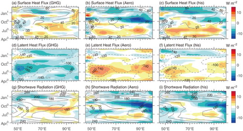
In terms of the historical simulation, the seasonal evolutions of these variables (Figs 7c, 7f, and 7i) tend to follow the patterns in the aerosol simulation, indicating the dominance of aerosol forcing.

c Subsurface Changes

Under GHG forcing, the anomalous warming generally decreases with depth (Figs 8a, 8d, and 8g), which leads to a more stratified upper ocean, especially over the ETIO (Figs 4j, 6a, and 8d). From June to August (Fig. 8(a)), the anomalous southeasterly winds, by preventing the intrusion of the eastward current and increasing upwelling, produce minimum warming in the subsurface ocean off Indonesia (Saji et al., 1999). As for the central and western regions, the intensified trade winds (i.e., anomalous easterlies along the equator in the zonal direction) increase the oceanic Ekman divergence and force upwelling Kelvin waves; anomalous westward flow transports water from east to west, thereby inducing upwelling off Sumatra to compensate for the loss; these consequences will lead to further subsurface cooling (i.e., minimum warming) and a shoaling thermocline in the east. On the other hand, weak westerly winds exist over the west from April to November (Fig. 6d), which induce an eastward flow that counteracts the westward flow from the central TIO. As a result, the thermocline depth over the west barely changes (Figs 8a and 8d). After November, strong westerly winds become dominant in the west, inducing eastward flow along the equator and flattening the thermocline in the east (Fig. 8g).

Fig. 8 Seasonal evolution of temperature anomalies (shading) and current anomalies (vectors) along the equator (averaged between 0.5°S and 0.5°N) in the GHG run (first column), aerosol run (second column), and historical run (last column): (a), (b), and (c) June–August of year 0; (d), (e), and (f) September–November of year 0; (g), (h), and (i) December of year 0 to February of year 1. The thermocline depth (thick lines) and the climatological temperature fields (thin lines) are superimposed. Thermocline depth is identified as the location of the maximum vertical gradient of the temperature.

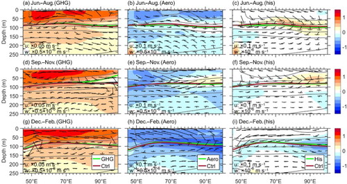
For aerosol forcing, the anomalous cooling decreases with depth from June to November (Figs 8b and 8e). With the aid of enhanced equatorial westerly winds from west to east from June to November (Fig. 6e), water converges around the equator and downwelling Kelvin waves are induced; eastward flow brings water volume to the east, thereby producing anomalous downwelling off Sumatra; these effects induce further subsurface warming and a deepening thermocline in the east. Meanwhile, the thermocline is uplifted slightly in the west to compensate for the upwelling, which is induced by anomalous westerlies. However, the background westerly wind reverses along the equatorial TIO by November (Fig. 6e), along with intensified anomalous easterly wind and upwelling (Fig. 6k), which may be induced by upwelling Kelvin waves, leading to a subsurface cooling anomaly and a shoaling thermocline in the eastern region, as well as subsurface warming and a deepening thermocline in the west (Fig. 8h). It's also notable that the change in thermocline depth is more sensitive to anomalous easterly winds than to westerlies (i.e., for the same one unit of zonal wind change, the amount of thermocline shoaling is far greater when anomalous easterly winds prevail than the amount of deepening induced by westerly wind anomalies, especially over the eastern region (compare Fig. 8d with 8e).

Another intriguing phenomenon is found in the two single-forcing simulations is that the profiles depict a large cooling (warming) anomaly between 50 and 200 m during the June–November period, which corresponds to a shoaling (deepening) of the thermocline over the ETIO under GHG (aerosol) forcing. The subsurface cooling (warming) anomaly associated with the warming (cooling) of the sea surface will result in an increase (a decrease) in the vertical stratification (Alory & Meyers, 2009). The intensified (reduced) stratification will further control the seasonal evolution of SSTAs as described in Section 4.b, indicative of the Bjerknes feedback. As Liu, Lu, and Xie (2015) suggested, the westward and downward-extending tongue-like subsurface cooling (warming), associated with the shoaling (deepening) thermocline and the easterly (westerly) anomaly, in the upper 100 m of the ocean off Sumatra, demonstrates the vital role of the Bjerknes feedback through wind-driven ocean circulation during both GHG forcing and aerosol forcing. Nevertheless, the magnitude of the thermocline shoaling in the GHG run is obviously larger than the magnitude of the deepening in the aerosol run. This leads to the situation in which the thermocline feedback greatly intensifies under GHG forcing, while the thermocline feedback weakens a little under aerosol forcing, another indication of the asymmetric response between the two radiative forcings.

As with the surface variables, the subsurface changes in the historical run are similar to those in the aerosol run, indicating that the aerosol effect exceeds the GHG effect not only for the sea surface but also for the subsurface ocean.

In short, this analysis finds that Bjerknes feedback plays a major role in regulating the life cycle of the IOD-like pattern through controlling ocean surface and subsurface changes in the ETIO. This positive feedback contributes to the anomalous cooling or warming off the coast of Sumatra during the September–November period; thereby, benefitting the growth as well as the collapse of the pIOD-like or nIOD-like SST pattern.

5 SST residual and IOD asymmetry

a Patterns

As described in the previous section, the climate response of the TIO to GHG- and aerosol-induced radiative forcings is not symmetric. The asymmetry is measured by the sum of the anomalies between these two scenarios, which is referred to as an anomaly residual. Figure 9a displays the spatial distribution of the SSTA residual, which features warming over the central and western TIO and a cooling off Sumatra. As a matter of fact, the amplitude of the SSTA asymmetry over the ETIO between the internal pIOD and nIOD is an important characteristic of IOD events, with the amplitude of the former being larger (Cai et al., 2012; Cai & Qiu, 2013; Hong et al., 2008; Zheng et al., 2010). To be clear, here we measure the asymmetry between the two phases of IOD events with the skewness of the ETIO SSTAs in the pre-industrial control experiment, following Zheng et al. (2010). The skewness is defined as(1) where is the th moment,(2) and is the th datum (seasonal mean), is the climatological mean of the control run, and is the number of data points.

Fig. 9 Horizontal distribution of the asymmetry over the Indian Ocean for the September–November period for (a) the SST residual between GHG and aerosol forcings and (b) the SST skewness between pIOD and nIOD events in the pre-industrial control experiment. The red rectangle indicates the ETIO region for the heat budget analysis.

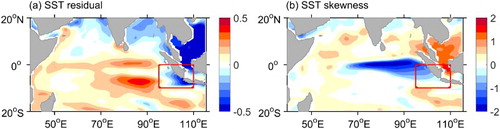
The horizontal distribution of the SST skewness in the Indian Ocean is shown in Fig. 9b. It is clear that a significant negative SST skewness occurs off Sumatra. Several possible mechanisms have been proposed to explain this negative SST skewness (Hong et al., 2008; Hong & Li, 2010; Zheng et al., 2010) although the root cause of the asymmetry is still being debated. Existing hypotheses may help uncover the physical processes that lead to the negative SST residual off Sumatra between GHG and aerosol forcings. To this end, we perform a mixed-layer heat budget analysis in the next section.

b Formation Mechanisms

To examine the relative roles of ocean dynamics and surface heat fluxes in causing the negative SST skewness between the two phases of the IOD events, as well as the negative SST residual between GHG and aerosol forcings, we perform a 0–55 m oceanic mixed-layer heat budget analysis over the ETIO region, following the method in Luo et al. (2016). It should be noted that the mixed-layer temperature (MLT), 0–55 m layer temperature, and SST have similar interannual variability; as a result, the fixed 0–55 m MLT change is a good representation of the SSTA. The MLT budget equation can be written as(3) where represents the MLT; denotes the MLT tendency, which goes to zero at interdecadal and longer time scales (Dong & Zhou, 2014; Xie et al., 2010); represents the net downward heat flux, in which and are the heat flux at the surface and shortwave radiation penetration at the bottom of the mixed layer, respectively, consists of the net downward shortwave radiation, longwave radiation, latent heat flux, and sensible heat flux at the sea surface. Furthermore, ( = 2850 J kg⁻¹ K⁻¹) and ( = 1025 ) are the specific heat and density of water, respectively; the oceanic temperature advection consists of zonal (), meridional (), and vertical () components, and each can be further divided into linear and non-linear parts:(4) In each equation the first two terms in parentheses on the right-hand side represent the linear dynamic heating (LDH), and the last term represents the non-linear dynamic heating (NDH); , , and are the zonal, meridional, and vertical velocities, respectively, averaged from the surface to the mixed-layer bottom, and the overbar and prime represent the climatological mean of the control run and the departure from mean, respectively; denotes the diffusion term, including ocean heat transport by unresolved processes and sub-monthly oceanic processes due to the monthly outputs and can be inferred as a residual term from Eq. (4); ( = 55 m) is the mixed-layer depth.

c Ocean Advection

Ocean advection tends to weaken the warming (cooling) under GHG (aerosol) forcing (Fig. 10a), with its amplitude being slightly larger under aerosol forcing (0.06°C mo⁻¹ than under GHG forcing (−0.05°C mo⁻¹). This difference will generate a positive SST residual over the ETIO. In more detail, the positive residual of advection primarily results from the stronger meridional and vertical advective warming under aerosol forcing than the advective cooling under GHG forcing (Fig. 10e). On the other hand, the negative zonal advection residual will produce a negative SST residual through stronger advective cooling under aerosol forcing but weaker warming under GHG forcing.

Fig. 10 Temperature advection, heat flux, and the residual term in the mixed-layer heat budget analysis over the ETIO (red box in Fig. 9) in (a) GHG and aerosol runs; (b) composite IOD events for the September–November period. Black bars represent the results from the GHG run (pIOD events) and grey bars from the aerosol run (nIOD events). The breakdown of the heat flux averaged over the ETIO under single forcing and composite IOD events are presented in (c) and (d), respectively. The breakdown of ocean temperature advection for single forcing and composite IOD events are presented in (e) and (f), respectively. Note that , and are the zonal, meridional, and vertical components of the advection, respectively, and LDH and NDH are the linear and non-linear components, respectively, and are composed of the zonal, meridional, and vertical parts (LDZ, LDM, and LDV for the LDH term; , , and for the NDH term), respectively.

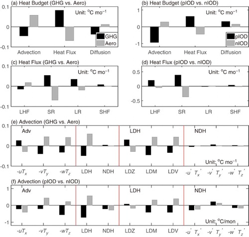
In terms of internal IOD events, however, stronger cold advection in pIOD (−0.93°C mo⁻¹) than in nIOD (0.29°C mo⁻¹) is the origin of the negative SST skewness over the ETIO (Fig. 10b). Further, the negative SST skewness is largely associated with the anomalous cold zonal advection by enhancing the anomalous cooling during pIOD and suppressing the warming during nIOD (Fig. 10f). Moreover, the vertical cooling being stronger in pIOD than the vertical warming in nIOD will also contribute to the negative SST skewness, whereas the meridional advection tends to reduce the negative SST skewness between the warm and cold episodes.

To further explore the role of ocean dynamics in causing the asymmetry, we separate the ocean temperature advections into its component parts: LDH terms and NDH terms as presented in Eq. (4). For both GHG and aerosol scenarios (Fig. 10e), the LDH term induces a positive residual because of a stronger warm linear advection in the aerosol scenario. This positive residual is primarily attributed to its zonal and vertical components, while the linear meridional term plays a role in causing the negative residual over the ETIO. On the other hand, the negative non-linear zonal and vertical advection residual will act to balance the asymmetry induced by the LDH, but its contribution to regulating the negative residual is almost negligible compared with the LDH terms.

For internal IOD events (Fig. 10f), the NDH acts to cool the SST in both the warm and cold episodes, suggesting that the asymmetric NDH effect on SST will contribute to the negative SST skewness (Cai et al., 2012; Cai & Qiu, 2013; Hong et al., 2008). Further analysis shows that both the non-linear zonal and vertical advections act to enhance the cold SST anomaly but damp the warm SST anomaly, thus favouring negative SST skewness in the ETIO. Meanwhile, the LDH tends to enhance the SST during both pIOD and nIOD events but with less warming during the negative events. The asymmetric response of all three LDH terms contributes to the negative SST skewness between pIOD and nIOD events.

In summary, under GHG and aerosol scenarios, the total oceanic advection that appears to be positive does not contribute to the formation of the negative SST residual. In stark contrast, the asymmetric change in the ocean advection between the two phases of the IOD events, due mainly to the zonal and vertical parts of the non-linear advection, as well as the linear advection, is the root of the negative SST skewness.

d Surface Heat Flux

During both GHG and aerosol forcings (Fig. 10a), the heat flux residual (0.01°C mo⁻¹) tends to enhance the warming effect from advection so does not contribute to the negative residual over the ETIO. During internal IOD events (Fig. 10b), the warming effect in the pIOD (0.62°C mo⁻¹) appears to be larger than the cooling effect (−0.44°C mo⁻¹) in the nIOD, also not favouring the negative SST skewness.

Further analysis of the surface heat flux finds that, under the GHG and aerosol scenarios (Fig. 10c), shortwave radiation contributes (−0.02°C mo⁻¹) to the negative SST residual, while longwave radiation does the reverse (0.02°C mo⁻¹). As discussed in Section 4.a, the anomalous negative shortwave radiation residual is mainly attributed to the asymmetric changes in cloud cover between the GHG and aerosol forcings, indicative of the cloud-radiation-SST feedback being a source of the negative residual over the ETIO. In addition to longwave radiation, the positive latent heat flux residual (0.004°C mo⁻¹) and sensible heat flux residual (0.008°C mo⁻¹) appear to be another damping source for the cold SST residual formation over the ETIO region.

For internal IOD events (Fig. 10d), however, the warming effect of shortwave radiation during a cold event (0.44°C mo⁻¹) is stronger than its cooling effect during a warm event (−0.38°C mo⁻¹), consistent with the findings of Ogata, Xie, Lan, and Zheng (2013). Thus, this kind of asymmetric damping will contribute to balancing the negative SST skewness, representing the opposite role of the cloud-radiation-SST feedback to the skewness formation. On the contrary, Hong et al. (2008) suggested that the cloud-radiation-SST feedback is another fundamental cause of the negative SST skewness over the ETIO because of its lower efficiency in damping the cold anomaly when it reaches critical amplitude. Cai et al. (2012) and Cai and Qiu (2013) provided another opinion, in which the threshold value for the cloud-radiation-SST feedback to reach cloud-free conditions is almost unattainable. In addition, they suggested that the ETIO IOD asymmetry occurs despite the stronger damping of negative SSTAs rather than by a breakdown of the cloud-radiation-SST feedback. Regarding the latent heat flux, it appears that a much larger warming effect during pIOD events than cooling effect during nIOD events, indicates its damping role for negative SST skewness.

e Diffusion

The diffusion term under GHG forcing (−0.03°C mo⁻¹) can produce much stronger cooling than the warming under aerosol forcing (0.01°C mo⁻¹) (Fig. 10a), indicative of the important role of the diffusion residual (−0.02°C mo⁻¹) in producing the negative SST residual over the ETIO. Because only monthly outputs are employed, the diffusion term in the heat budget consists of heat transport by sub-monthly oceanic processes and other unresolved processes in the model, such as eddy diffusion and eddy transport. For internal IOD events (Fig. 10b), however, the diffusion has a warming effect during pIOD events but a cooling effect during nIOD events, with the former being much larger than the latter.

6 Discussion

Under GHG and aerosol forcings, changes in the ocean circulation may be related to changes in the ITF. We calculate the annual ITF transport in the three major exit passages of Lombok Strait, Ombai Strait, and Timor Passage, and the total transport from the three passages into the Indian Ocean is 16.7 Sv (1 Sv = 10⁶ m³) in the control run, 15.5 Sv in the GHG run, and 17.5 Sv in the aerosol run, which are comparable to 15.0 Sv from the transport estimated by Sprintall, Wijffels, Molcard, and Jaya (2009) based on their observations. Therefore, the ITF transport increases by 0.8 Sv (4.8%) in the aerosol run but decreases by 1.2 Sv (7.2%) in the GHG run compared with the control run, consistent with the findings of Collier, Rotstayn, Kim, Hirst, and Jeffrey (2013). The assymetrical changes in ITF transport are related to the different mean state between the GHG and aerosol simulations. As shown in Section 4, the GHG (aerosol) simulation is accompanied by a slowdown in (acceleration of) the Walker circulation, which would weaken (strengthen) the easterlies in the tropical Pacific, thereby, leading to a weaker (stronger) warming over the western tropical Pacific and reduced (enhanced) ITF transport. Because the ITF carries warm water from the western Pacific into the Indian Ocean (Song, Vecchi, & Rosati, 2007), the aerosol-induced higher ITF transport will warm the upper ocean and deepen the thermocline in the ETIO, whereas the lower ITF transport induced by GHGs will cool the upper ocean and elevate the thermocline in the ETIO. As a result, the asymmetrical change in the ITF transport between the GHG run and the aerosol run can contribute to thermocline shoaling induced by GHGs being stronger than its deepening by aerosols.

7 Conclusions

Based on the historical single-forcing and all-forcing simulations from GFDL CM3, we have compared the climate response patterns over the TIO under GHG and aerosol forcings. Results show that, although the GHG forcing induces a pIOD-like SST response, the mean climate conditions over the TIO shift toward an nIOD-like state under aerosol forcing. The GHG-induced pIOD-like warming pattern features a reduction in (enhancement of) SST warming in the ETIO (WTIO) and anomalous easterlies along the equator, as well as a shallower thermocline in the ETIO. The aerosol-induced nIOD-like pattern is characterized by a reduction in (enhancement of) SST cooling over the ETIO (WTIO), westerly anomalies around the equator, and a deepening of the thermocline off the coast of Sumatra. Although the latter appears to be a reversal of the former, strong asymmetry is found in the SST changes. In particular, the cooling response to the aerosol forcing exceeds the warming response to GHG forcing off Sumatra, leading to a negative SST residual there.

Because negative SST skewness is also found between the two phases of IOD events, we performed a mixed-layer heat budget analysis over the ETIO region to examine the differences in the physical processes producing the negative SST residual and the negative SST skewness. To summarize, we found that

• Under GHG and aerosol forcing, the total ocean advection has a positive residual and thus damps the negative SST residual although the zonal advection term is negative and favourable to formation of the negative residual. Under pIOD and nIOD, in contrast, the asymmetric response of ocean advection is the cause of the negative SST skewness.

• Under both GHG and aerosol forcing, the surface heat flux residual is positive. Among its four components, however, the shortwave radiation residual is negative and contributes to the negative SST residual. Under pIOD and nIOD, the opposite occurs, and asymmetric shortwave radiation and latent heat flux changes act to damp the formation of negative SST skewness.

• The diffusive residual under GHG and aerosol forcing is negative and thus contributes to the negative SST residual. In contrast, the diffusion term in pIOD events appears to be positive and much larger than the negative diffusion in nIOD events, thus working to suppress the formation of negative SST skewness.

It should be mentioned that our study is limited in that it relies on only one model, the results could, therefore, be model-dependent. For example, large uncertainty has been found in the magnitude and spatial pattern of anthropogenic aerosol forcing among the CMIP5 models (e.g., Rotstayn et al., 2012). Therefore, the response of the TIO to aerosol forcing may feature large inter-model diversity. Further research is needed using a range of climate models within the CMIP5 framework to better understand the mechanisms and the extent to which the findings of the present study are model-dependent.

Acknowledgements

We are grateful for the constructive criticism and comments from two anonymous reviewers, which greatly improved the paper.

Disclosure statement

No potential conflict of interest was reported by the authors.

Additional information

Funding

This research is supported by the National Natural Science Foundation of China [grant number 41676002] and [grant number 41376009], as well as the Strategic Priority Research Program of the Chinese Academy of Sciences [grant number XDA11010302].

References

- Alory, G., & Meyers, G. (2009). Warming of the upper equatorial Indian Ocean and changes in the heat budget (1960–99). Journal of Climate, 22(1), 93–113. doi: 10.1175/2008jcli2330.1
- Bjerknes, J. (1969). Atmospheric teleconnections from the equatorial Pacific. Monthly Weather Review, 97, 163–172. doi: 10.1175/1520-0493(1969)097<0163:ATFTEP>2.3.CO;2
- Boucher, O., Randall, D., Artaxo, P., Bretherton, C., Feingold, G., Forster, P., … Zhang, X. Y. (2013). Clouds and aerosols. In T. F. Stocker, D. Qin, G.-K. Plattner, M. Tignor, S. K. Allen, J. Doschung, A. Nauels, Y. Xia, V. Bex, & P. M. Midgley (Eds.), Climate change 2013: The physical science basis. Contribution of Working Group I to the Fifth Assessment Report of the Intergovernmental Panel on Climate Change (pp. 571–657). Cambridge: Cambridge University Press. doi: 10.1017/CBO9781107415324.016
- Cai, W., & Cowan, T. (2013). Why is the amplitude of the Indian Ocean Dipole overly large in CMIP3 and CMIP5 climate models? Geophysical Research Letters, 40(6), 1200–1205. doi: 10.1002/grl.50208
- Cai, W., Cowan, T., & Raupach, M. (2009). Positive Indian Ocean Dipole events precondition southeast Australia bushfires. Geophysical Research Letters, 36(19), L19710. doi: 10.1029/2009gl039902
- Cai, W., Cowan, T., & Sullivan, A. (2009). Recent unprecedented skewness towards positive Indian Ocean Dipole occurrences and its impact on Australian rainfall. Geophysical Research Letters, 36(11), L11705. doi: 10.1029/2009gl037604
- Cai, W. J., Zheng, X. T., Weller, E., Collins, M., Cowan, T., Lengaigne, M., & Yamagata, T. (2013). Projected response of the Indian Ocean Dipole to greenhouse warming. Nature Geoscience, 6, 999–1007. doi: 10.1038/ngeo2009
- Cai, W., & Qiu, Y. (2013). An observation-based assessment of nonlinear feedback processes associated with the Indian Ocean Dipole. Journal of Climate, 26(9), 2880–2890. doi: 10.1175/jcli-d-12-00483.1
- Cai, W., Santoso, A., Wang, G., Weller, E., Wu, L., Ashok, K., … Yamagata, T. (2014). Increased frequency of extreme Indian Ocean Dipole events due to greenhouse warming. Nature, 510(7504), 254–258. doi: 10.1038/nature13327
- Cai, W., van Rensch, P., Cowan, T., & Hendon, H. H. (2012). An asymmetry in the IOD and ENSO teleconnection pathway and its impact on Australian climate. Journal of Climate, 25(18), 6318–6329. doi: 10.1175/jcli-d-11-00501.1
- Collier, M. A., Rotstayn, L. D., Kim, K.-Y., Hirst, A. C., & Jeffrey, S. J. (2013). Ocean circulation response to anthropogenic aerosol and greenhouse gas forcing in the CSIRO-Mk3.6 coupled climate model. Australian Meteorological and Oceanographic Journal, 63(1), 27–39. doi: 10.22499/2.6301.003
- Cowan, T., Cai, W., Ng, B., & England, M. (2015). The response of the Indian Ocean Dipole asymmetry to anthropogenic aerosols and greenhouse gases. Journal of Climate, 28(7), 2564–2583. doi: 10.1175/jcli-d-14-00661.1
- Dong, L., & Zhou, T. (2014). The Indian Ocean sea surface temperature warming simulated by CMIP5 models during the twentieth century: Competing forcing roles of GHGs and anthropogenic aerosols. Journal of Climate, 27(9), 3348–3362. doi: 10.1175/jcli-d-13-00396.1
- Donner, L. J., Wyman, B. L., Hemler, R. S., Horowitz, L. W., Ming, Y., Zhao, M., … Zeng, F. (2011). The dynamical core, physical parameterizations, and basic simulation characteristics of the atmospheric component AM3 of the GFDL global coupled model CM3. Journal of Climate, 24(13), 3484–3519. doi: 10.1175/2011jcli3955.1
- Griffies, S. M., Winton, M., Donner, L. J., Horowitz, L. W., Downes, S. M., Farneti, R., … Zadeh, N. (2011). The GFDL CM3 coupled climate model: Characteristics of the ocean and sea ice simulations. Journal of Climate, 24(13), 3520–3544. doi: 10.1175/2011jcli3964.1
- Hong, C.-C., & Li, T. (2010). Independence of SST skewness from thermocline feedback in the eastern equatorial Indian Ocean. Geophysical Research Letters, 37(11), L11702. doi: 10.1029/2010gl043380
- Hong, C.-C., Li, T., Ho, L., & Kug, J.-S. (2008). Asymmetry of the Indian Ocean Dipole. Part I: Observational analysis. Journal of Climate, 21(18), 4834–4848. doi: 10.1175/2008jcli2222.1
- Ihara, C., Kushnir, Y., & Cane, M. A. (2008). Warming trend of the Indian Ocean SST and Indian Ocean Dipole from 1880 to 2004. Journal of Climate, 21(10), 2035–2046. doi: 10.1175/2007jcli1945.1
- Li, T., Wang, B., Chang, C.-P., & Zhang, Y. (2003). A theory for the Indian Ocean Dipole-zonal mode. Journal of the Atmospheric Sciences, 60, 2119–2135. doi: 10.1175/1520-0469(2003)060<2119:ATFTIO>2.0.CO;2
- Liu, F., Luo, Y., Lu, J., Garuba, O., & Wan, X. (2017). Asymmetric response of the equatorial Pacific SST to climate warming and cooling. Journal of Climate, 30(18), 7255–7270. doi: 10.1175/jcli-d-17-0011.1
- Liu, W., Lu, J., & Xie, S.-P. (2015). Understanding the Indian Ocean response to double CO2 forcing in a coupled model. Ocean Dynamics, 65(7), 1037–1046. doi: 10.1007/s10236-015-0854-6
- Luo, Y., Lu, J., Liu, F., & Wan, X. (2016). The positive Indian Ocean Dipole–like response in the tropical Indian Ocean to global warming. Advances in Atmospheric Sciences, 33(4), 476–488. doi: 10.1007/s00376-015-5027-5
- Ng, B., Cai, W., & Walsh, K. (2014). Nonlinear feedbacks associated with the Indian Ocean Dipole and their response to global warming in the GFDL-ESM2M coupled climate model. Journal of Climate, 27(11), 3904–3919. doi: 10.1175/jcli-d-13-00527.1
- Ogata, T., Xie, S.-P., Lan, J., & Zheng, X. (2013). Importance of ocean dynamics for the skewness of the Indian Ocean Dipole mode. Journal of Climate, 26(7), 2145–2159. doi: 10.1175/jcli-d-11-00615.1
- Rotstayn, L. D., Jeffrey, S. J., Collier, M. A., Dravitzki, S. M., Hirst, A. C., Syktus, J. I., & Wong, K. K. (2012). Aerosol- and greenhouse gas-induced changes in summer rainfall and circulation in the Australasian region: A study using single-forcing climate simulations. Atmospheric Chemistry and Physics, 12(14), 6377–6404. doi: 10.5194/acp-12-6377-2012
- Saji, N. H., Goswami, B. N., Vinayachandran, P. N., & Yamagata, T. (1999). A dipole mode in the tropical Indian Ocean. Nature, 401, 360–363. doi: 10.1038/43854
- Song, Q., Vecchi, G. A., & Rosati, A. J. (2007). The role of the Indonesian throughflow in the Indo–Pacific climate variability in the GFDL coupled climate model. Journal of Climate, 20(11), 2434–2451. doi: 10.1175/jcli4133.1
- Sprintall, J., Wijffels, S. E., Molcard, R., & Jaya, I. (2009). Direct estimates of the Indonesian throughflow entering the Indian Ocean: 2004–2006. Journal of Geophysical Research, 114(C7), 114, C07001. doi: 10.1029/2008jc005257
- Taylor, K. E., Stouffer, R. J., & Meehl, G. A. (2012). An overview of CMIP5 and the experiment design. Bulletin of the American Meteorological Society, 93(4), 485–498. doi: 10.1175/bams-d-11-00094.1
- Wallace, J. M., & Hobbs, P. V. (2006). Atmospheric science: An introductory survey (2nd ed.). Salt Lake City, USA: Academic Press.
- Wang, H., Xie, S.-P., & Liu, Q. (2016). Comparison of climate response to anthropogenic aerosol versus greenhouse gas forcing: Distinct patterns. Journal of Climate, 29(14), 5175–5188. doi: 10.1175/jcli-d-16-0106.1
- Weller, E., & Cai, W. (2013). Realism of the Indian Ocean Dipole in CMIP5 models: The implications for climate projections. Journal of Climate, 26(17), 6649–6659. doi: 10.1175/jcli-d-12-00807.1
- Xie, S.-P., Deser, C., Vecchi, G. A., Ma, J., Teng, H., & Wittenberg, A. T. (2010). Global warming pattern formation: Sea surface temperature and rainfall. Journal of Climate, 23(4), 966–986. doi: 10.1175/2009jcli3329.1
- Xie, S.-P., Lu, B., & Xiang, B. (2013). Similar spatial patterns of climate responses to aerosol and greenhouse gas changes. Nature Geoscience, 6, 828–832. doi: 10.1038/NGEO1931
- Zheng, X.-T., Xie, S.-P., Du, Y., Liu, L., Huang, G., & Liu, Q. (2013). Indian Ocean Dipole response to global warming in the CMIP5 multimodel ensemble. Journal of Climate, 26(16), 6067–6080. doi: 10.1175/jcli-d-12-00638.1
- Zheng, X.-T., Xie, S.-P., Vecchi, G. A., Liu, Q., & Hafner, J. (2010). Indian Ocean Dipole response to global warming: Analysis of ocean–atmospheric feedbacks in a coupled model. Journal of Climate, 23(5), 1240–1253. doi: 10.1175/2009jcli3326.1