Wind Waves in the Strait of Georgia

ABSTRACT

The Strait of Georgia, British Columbia, Canada, is an important ocean region in which wave and weather conditions can vary rapidly in time and space because of the complex mountain topography that surrounds it. Here we analyze existing observational data and a newly developed near real-time numerical wave model, forced by modelled local winds and ocean currents, to characterize the surface wave conditions of the Strait under a variety of wind and weather conditions. Wave heights are generally largest in the northern Strait. However, we find that there are some deficiencies in the existing observational data, with buoy measurements in the northern Strait overestimating wave heights by as much as 0.4 m. The wave modelling also shows that strong tidal flows near Discovery Passage and Boundary Pass lead to increased wave heights, but current-related increases are not predicted near Sand Heads because of deficiencies in the numerical ocean current model. Outflow wind conditions in the Fraser Valley result in large waves south of Point Roberts but Howe Sound outflows do not noticeably affect significant wave heights offshore of Howe Sound. Stokes drift associated with surface waves can cause surface drifts as large as 20% of the directly wind-driven surface currents but is minimal for winds less than about $5\mathrm{m}{\mathrm{s}}^{-1}$, which characterize the Strait most of the time. Whitecap fractions throughout the Strait are similar to open-ocean conditions (i.e., 1–2% at moderate wind speeds) but about twice as high in the southern region of the Strait during strong outflow conditions.

RÉSUMÉ

[Traduit par la rédaction] En raison de la topographie complexe des montagnes qui l'entourent, le détroit de Georgia, en Colombie-Britannique (Canada), constitue une importante région océanique dans laquelle les vagues et les conditions météorologiques peuvent rapidement changer dans le temps et dans l'espace. Nous analysons ici des données d'observation existantes et un nouveau modèle numérique de vagues en temps quasi réel, forcé par des vents locaux et des courants océaniques modélisés, et ce, afin de caractériser les conditions de vagues à la surface du détroit selon diverses conditions météorologiques, dont le vent. Les hauteurs de vagues s'avèrent généralement les plus élevées dans le nord du détroit. Cependant, nous constatons que les données d'observation existantes présentent certaines anomalies. Les mesures qu'enregistrent les bouées dans le nord du détroit surestiment jusqu'à 0,4 m la hauteur des vagues. La modélisation des vagues montre également que les forts courants de marée près des passages Discovery et Boundary entraînent une augmentation de la hauteur des vagues, mais les augmentations liées aux courants ne sont pas prévues près de Sand Heads en raison des lacunes du modèle numérique des courants marins. Les vents sortants de la vallée du Fraser génèrent de hautes vagues au sud de Point Roberts, mais les vents sortants de la baie Howe n'affectent pas vraiment la hauteur des vagues au large de cette baie. La dérive de Stokes associée aux vagues de surface peut provoquer des dérives en surface s'élevant à au moins 20 superficiels directement dus au vent, mais celles-ci restent minimes pour les vents de moins de 5 m s^-1 environ, qui caractérisent le détroit la plupart du temps. Le pourcentage des vagues à crête blanche dans l'ensemble du détroit correspond à celui de la haute mer (c'est-à-dire 1 à 2% pour des vitesses de vent modérées), mais est environ deux fois plus élevé dans la région sud du détroit en cas de forts vents sortants.

KEYWORDS:

• surface waves
• coastal strait
• Strait of Georgia
• WAVEWATCH III®
• spatial wave characteristics
• buoy-model comparison
• NEMO

1 Introduction

The Strait of Georgia is an inland sea about 200 km long and 30 km wide, with maximum depths close to 450 m (Fig. 1). The Strait is located mostly in Canada although the southernmost tip is in US waters, and about 10% of Canada's population lives on the shores of the Strait and on islands within it. The waters of the Strait are heavily used for recreational and commercial purposes. This includes traffic to and from the Port of Vancouver, the largest port in Canada, as well as vehicle ferry traffic across the Strait ($\sim 80$ sailings per day).

Fig. 1 (a) Location of the Strait of Georgia and WW3 mode domain. (b) Strait of Georgia. Shading indicates coastline, 500 m, and 1000 m elevation contours.

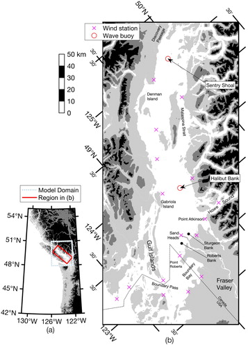
However, because of the rugged mountain topography of the area, with elevations of more than 1000 m closely bordering the coast, weather conditions around the Strait of Georgia can vary spatially. There are more than a dozen government weather stations on coasts and islands in the Strait area, as well as two moored weather buoys that record hourly atmospheric conditions and ocean surface wave spectra (Fig. 1b). Wind and wave conditions can vary rapidly in time from flat calm to storms severe enough that the 200 m–long vessels of the BC Ferries fleet are sometimes unable to dock until seas subside. Experienced sailors also know that Strait conditions can vary greatly over short spatial scales, especially when waves propagate into areas of strong opposing currents. The confused seas near the Fraser River's outflow at Sand Heads contributed to the capsizing of the fishing vessel Cap Rouge II with the loss of five lives in 2002 (Transportation Safety Board of Canada [TSB], 2003).

Surface wave conditions in the Strait of Georgia also contribute to the resuspension of sediment on Sturgeon Bank and Roberts Bank at the mouth of the Fraser River (Hill & Davidson, 2002) and are an important factor governing the operating range of a high-frequency radar array in the southern Strait (Halverson, Pawlowicz, & Chavanne, 2017). The Stokes drift from surface waves may also be an important factor governing the dispersal of floating objects (Farazmand & Sapsis, 2019). On the other hand, wave contributions to mixing and momentum in the Fraser River plume are generally small (Kastner, Horner-Devine, & Thomson, 2018).

Recently, a WAVEWATCH III^® numerical wave model with a 500 m grid for the Strait of Georgia was configured to run in conjunction with a real-time Nucleus for European Modelling of the Ocean (NEMO) now-cast model of ocean conditions, and a 2.5 km resolution atmospheric model. Here we evaluate the existing observational data, as well as the one-way coupled wind–wave–current model, by comparison with existing wave data. Then we use wave model output from 2017 to 2019 to characterize the surface wave conditions of the Strait under a variety of wind and weather conditions. Our analysis of Strait conditions is complementary to a similar analysis recently carried out for wave conditions in the Salish Sea area using a wind–wave model coupled to open ocean wave conditions, concentrating on the propagation of ocean swell into, and the wave climate of, Juan de Fuca Strait and Puget Sound (Yang, Garcia-Medina, Wu, Wang, & Mauger, 2019).

2 Methods

a Observations

Near-real-time wave and wind records at hourly intervals in the Strait of Georgia are available at two 3 m discus weather buoys from AXYS Technologies Inc.: C46131 Sentry Shoal and C46146 Halibut Bank (Fig. 1, red circles), which are owned and operated by a branch of the Canadian government (Environment and Climate Change Canada; ECCC). Wind speed at these buoys is measured at 5 m above sea level, giving speeds that are 94% of $U_{10}$, the wind at the standard reference height of 10 m (using a log-layer parameterization in conditions of neutral stability). Along with Large & Pond (1981) and Pawlowicz, Beardsley, Lentz, Dever, & Anis (2001), we use this factor to estimate $U_{10}$ when needed. One-dimensional wave spectra $S\left(f\right)$, giving variance density of the sea surface elevation as a function of frequency f, are generated hourly by double integration of observations from a fixed accelerometer over a period of 38 min. Spectral information is provided for 41 frequency bands with periods $T=1/f$ between 2.2 and 256 s. Significant wave height $H_s$ and peak wave period $T_p$ are calculated from this spectral information using proprietary buoy software and are provided in near real-time to a precision of one decimal place (i.e., 0.1 m and 0.1 s respectively).

Buoy observations are transmitted through the Global Telecommunications System (GTS) and are archived by the Marine Environmental Data Section of Fisheries and Oceans Canada (DFO). These archived data have undergone some standard quality-control procedures at DFO. Wave height and period parameters are recalculated; the recalculated wave heights are presented to a precision of two decimal places (0.01 m), which results in figures with less obvious quantization of the wave parameters. However, data quality for these recalculated values is uncertain (possibly lower) and the values have not been well calibrated (B. Bradshaw, DFO, personal communication, 2019). Although 54% of the wave data at C46131 are flagged as “record appears erroneous,” and at C46146 this rate is 16% (in comparison with rates for offshore buoys that are more typically $\ll 1$%), these flags are generated in an automated process and probably reflect a dissimilarity with typical open ocean conditions rather than any intrinsic problem. However, it does suggest that data should be treated with some caution.

b Numerical modelling

Wave conditions are generated by WAVEWATCH III^® (model version 5.16), a third-generation spectral wave model developed by an international science community (The WAVEWATCH III^® Development Group, 2016). The model is applied in a forecast mode. Open water physics are represented with the default values of the ST4 parameterizations (Ardhuin et al., 2010). The model resolves 24 directional bins and 25 frequency bins with corresponding periods of 1.5 to 15 s. The bathymetry grid used for the run of this model is a 500 m resolution rectilinear grid based on a blend of the 1 arc-minute global relief ETOPO1 (NCEP, 2016) and survey data from the Canadian Hydrographic Service. The grid spans the region ${122}^{\circ }-{126}^{\circ }\mathrm{W}$ and ${48}^{\circ }-{50.5}^{\circ }\mathrm{N}$ in a $572\times 661$ grid (Fig. 1a). Only the local wind sea can be calculated, so the model outputs in regions with significant swell components (i.e., those more exposed to the open ocean) are an incomplete representation of the wave field. However, the Strait of Georgia is sheltered from ocean swell (Yang et al., 2019); hence, this is not a problem for the analysis carried out here.

The wave model is forced with surface winds derived from ECCC's 2.5 km resolution High Resolution Deterministic Prediction System (HRDPS) atmospheric model (Milbrandt et al., 2016) and ocean currents at 0.5 m depth obtained from SalishSeaCast, a NEMO 3.6 configuration (Soontiens & Allen, 2017; Soontiens et al., 2016) with a horizontal resolution of about 500 m. The water level is held constant. Both wind and surface current fields are interpolated onto the wave model grid. SalishSeaCast and the wave model are run in real time, multiple times daily using the Salish Sea Nowcast System (salishsea-nowcast.readthedocs.io) by the Allen group of the University of British Columbia (salishsea.eos.ubc.ca/nemo/). Since April 2017, the model has produced daily wave forecasts for a 60 h forecast period, at 10 min resolution. The model is initialized with the 24 h nowcast of the previous day, and the first 24 h of the new forecast is considered the nowcast for today.

Output of SalishSeaCast and the wave model are available at salishsea.eos.ubc.ca/erddap. Here, we analyze the first two years (i.e., 12 April 2017 to 11 April 2019) of daily model data at 1 h resolution from the wave model nowcast to extract typical spatial wave field characteristics. In addition, full resolution time series at point locations are utilized to gain information on the temporal evolution of waves in the Strait of Georgia. Wave model data interpolated onto the location and time stamps of the buoy observations are the basis for model evaluation.

3 Results

a Wave buoy measurements

First, we evaluate the uncertainties in the significant wave height values provided in the archived buoy data. These heights are calculated from the observed spectral information, so we begin by examining these spectra.

Wave spectra at both Sentry Shoal and Halibut Bank generally show a peak at frequencies $f_{\mathrm{p}\mathrm{e}\mathrm{a}\mathrm{k}}$ between 0.16 and 0.4 Hz, corresponding to wave periods between 2.5 and 6.5 s (Fig. 2).

Fig. 2 Wave spectra from (a) Halibut Bank and (b) Sentry Shoal, plotted on a log/log scale. Curves are observations taken every 100 h over the period of data availability. The dashed red line shows the universal high-frequency tail of the Pierson–Moskowitz spectrum, which is commonly used as a standard description of saturated wind-waves. The blue line shows an $f^{-4}$ dependence with an arbitrary height scaling.

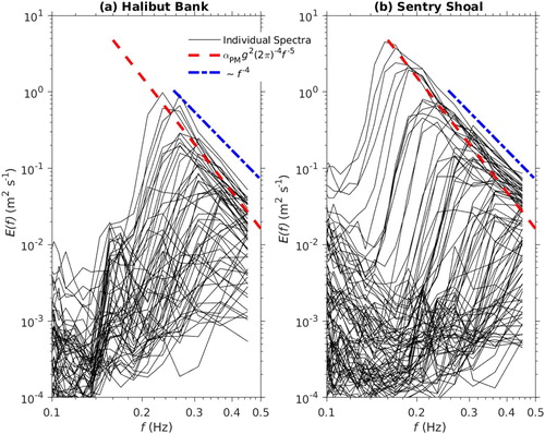
At frequencies above this peak the spectrum decreases in a relatively consistent way. The Pierson–Moskowitz wave spectrum $S_{\mathrm{P}\mathrm{M}}\left(f\right)$ for a fully-developed wind sea has a high-frequency tail above the peak in the form:(1) $S_{\mathrm{P}\mathrm{M}}\left(f\right)\sim \alpha g^2(2\pi {)}^{-4}{f}^{-5},\mathrm{f}\mathrm{o}\mathrm{r}f\gg f_{\mathrm{p}\mathrm{e}\mathrm{a}\mathrm{k}},$(1) where $\alpha \approx 0.0081$ is a universal constant, and g is the acceleration due to gravity (Holthuijsen, 2007). This power-law tail matches the upper envelope of the observed spectra reasonably well (within a factor of $\sim 3$) for frequencies larger than $f_{\mathrm{p}\mathrm{e}\mathrm{a}\mathrm{k}}$. Closer examination of raw spectra suggests that slightly better fits to the slopes of higher frequencies of individual spectra might be obtained with a decrease proportional to $f^{-4}$, typical for a so-called equilibrium wind sea (Phillips, 1985), although the overall spectral levels computed using a universal scaling of that form, described by Battjes, Zitman, and Holthuijsen (1987), do not match well. In the equilibrium range (i.e., at frequencies between $1.5f_{\mathrm{p}\mathrm{e}\mathrm{a}\mathrm{k}}$ and $3f_{\mathrm{p}\mathrm{e}\mathrm{a}\mathrm{k}}$) the wave spectrum scales as $f^{-4}$ and transitions to $f^{-5}$ at higher frequencies (Janssen, 2004). In the observed wave buoy spectra the transition frequency is not known, but it lies well outside the resolved part of the spectrum. Therefore, the unresolved energy will likely be dominated by the $f^{-4}$ scaling.

At frequencies below the spectral peak, the wave energy usually decreases rapidly, reaching a minimum at periods of around 5–8 s (frequencies of 0.125–0.2 Hz). Spectral energies then increase again at lower frequencies. The spectral energy at frequencies below the minimum arises from tethered mooring dynamics (including pitch, roll, and surface current effects), hence, does not reflect the true wave spectrum. The Halibut Bank buoy also has a sharp spectral peak at about 0.16–0.18 Hz (Fig. 2a), which appears on a regular schedule when spectral levels are low, and this peak is presumably related to details of the mooring and its instrumentation as well.

A common measure of wave height is the significant wave height $H_s$, which can be theoretically determined from the non-directional wave spectrum using the following definition:(2) $H_s=4\sqrt{{\int }_{f_0}^{f_1}S\left(f\right)\mathrm{d}f},$(2) where $f_0=0$ and $f_1\to \mathrm{\infty }$ (Holthuijsen, 2007). However, for practical calculations from buoy data the lower limit of integration $f_0$ is chosen to be some non-zero value to avoid including the spurious mooring energy at very low frequencies. Typically, for the Strait of Georgia this lower limit is most usefully taken to be at the spectral minimum at periods of about 5–8 s. Calculations by DFO (code VCAR in archived data) use a lower limit of 30 s, which will, therefore, tend to bias calculated wave heights upwards; buoy on-board calculations (code VWH$) appear to use a higher limit, but because of the quantization of the values reported, it is difficult to determine what this limit is. The spectral minimum appears at much higher frequencies for the Strait of Georgia buoys than on outer coast buoys, where it can be seen more typically at $\approx 0.04\mathrm{H}\mathrm{z}$ ($\approx 25\mathrm{s}$), and this different location of the minimum is possibly the source of the larger percentage of flagged data compared with offshore buoys.

In addition, the upper limit of integration $f_1$ is taken as $f_{max}=0.45\mathrm{H}\mathrm{z}$ for both on-board calculations and DFO post-processing. Higher-frequency energy is not accounted for, and this will tend to bias calculated wave heights downward. In either case, a significant part of the wave spectrum, with frequencies greater than $f_{max}$, is not included in calculations, and this may lead to a bias in reported wave heights, especially at low wind speeds, which are both quite frequent in the Strait of Georgia and are associated with high peak frequencies in the wave field. We estimate the unresolved portion of the spectrum by extrapolating from $S\left(f_{max}\right)$, the spectral measurement available at $f_{max}$, using(3) $S\left(f\right)=S\left(f_{max}\right){\left(\frac{f}{f_{max}}\right)}^{-4},f>f_{max}.$(3) Using Eq. (3(3) $S\left(f\right)=S\left(f_{max}\right){\left(\frac{f}{f_{max}}\right)}^{-4},f>f_{max}.$(3) ) to estimate the unresolved high-frequency part of the spectrum and choosing $f_0$ more carefully at 0.1 Hz, we find that the overall effect is that estimates of $H_s$ provided from the archive for Halibut Bank are generally too low by up to 0.1 m for wave heights greater than 0.2 m (because of the unresolved high frequencies) but are slightly too high for lower wave heights (because of the addition of spurious low-frequency energy). This is true for both on-board and post-processed wave heights. At Sentry Shoal the error is similar for on-board calculations, but for DFO calculations the results are somewhat different. These post-processed significant wave heights are roughly unbiased for wave heights less than about 2 m, but at greater heights these calculated wave heights are biased too high by as much as 0.4 m. A wave height of zero is rarely reported even in flat calm conditions.

In addition to $H_s$, a maximum height $H_{max}$ of individual waves within the sampling period (based on the range between zero-crossings of the sea surface height) is also recorded at the wave buoys. The hourly values of $H_s$ and $H_{max}$ are based on $\approx 700$ waves, and the Rayleigh distribution valid for a linear, narrow-banded wave field gives $H_{max}\approx 1.8H_s$ (Gemmrich & Garrett, 2011). For Halibut Bank we find empirically that for $H_s\ge 1\mathrm{m}$, $H_{max}\approx (1.71\pm 0.24)H_s$, whereas at Sentry Shoal $H_{max}\approx (1.96\pm 0.56)H_s$. Thus, extreme waves at Halibut Bank are consistent with the assumption of linear superposition. At Sentry Shoal the largest dominant waves may be affected by the shallow depths because $k_{p}d\approx 1$, where $k_p$ is the wavenumber of waves with peak spectral frequency, and $d=14\mathrm{m}$ is the water depth at the buoy. The shallow depth can introduce focusing of the wave field resulting in higher extremes (Janssen & Herbers, 2009). However, the highest values $H_{max}=2.52H_s$ are likely spurious.

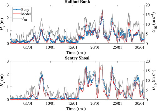
Now that we have evaluated the uncertainty in buoy estimates of $H_s$, we can consider their relationship to local winds. Examination of wind and wave height time series (e.g., Fig. 3) clearly shows a correlation.

Fig. 3 Comparison of the significant wave height $H_s$ from the wave model and the buoy observations January 2018. Both data are at the same hourly resolution. The grey lines depict the model wind speed $U_{10}$. Top: results for Halibut Bank in the central Strait of Georgia. Bottom: results for Sentry Shoal in the northern Strait of Georgia.

In fully-developed wind seas the significant wave height can be estimated from the wind speed $U_{10}$ at a reference height of 10 m through a quadratic relationship:(4) $H_s\approx A\frac{U_{10}^2}{g},$(4) with $A\approx 0.24$ (Holthuijsen, 2007). Local winds and waves at the two buoys are well correlated, but a least-squares fit finds much smaller wave heights for a given wind, with $A\approx 0.07$ for Halibut Bank and $A\approx 0.09$ for Sentry Shoal. The wave fields in the Strait of Georgia are fetch limited and are always young. Additionally, the steering effect of the narrow Strait also affects the fetch evolution (e.g., Pettersson, Kahma, & Tuomi, 2010). Therefore, we expect significant spatial variability of the wave field in the Strait of Georgia.

Quadratic fits of the form of Eq. (4(4) $H_s\approx A\frac{U_{10}^2}{g},$(4) ) yield reasonable predictions of wave height as a function of wind speed at each location, but there is often a lag of 1–3 h between a change in wind speed and the corresponding wave response (not very clearly shown in Fig. 3). Again, this is likely an effect of the fetch limitation. Winds of $\approx 10\mathrm{m}{\mathrm{s}}^{-1}$ will tend to generate waves with the same phase speed and a corresponding group speed of half that magnitude (i.e., $\approx 5\mathrm{m}{\mathrm{s}}^{-1}$). These will take about 3 h to travel 50 km. However, the spectrum of significant wave height, like that of the forcing winds, is dominated by a broad peak of variability with periods of 1–5 days. The effect of a lag of a few hours on changes that occur over a day or more is relatively small, so we ignore it in the rest of our analysis, treating the system response as quasi-steady.

b Model/Buoy Comparison

Spectral wave models achieve remarkable skill under open ocean conditions. However, in coastal and semi-enclosed seas the wave forecasts are less accurate, mainly because of uncertainties in the forcing wind field, stronger currents, and complex topography (Cavaleri et al., 2018). Furthermore, uncertainties in the in situ observations, as discussed above, might also contribute to the greater scatter between model and observations in coastal seas.

A one-month comparison of the model $H_s$ and the buoy observations at Halibut Bank and Sentry Shoal in January 2018 (Fig. 3) shows that the model generally captures the magnitude and timing of all main wave events reasonably well (here we use the significant wave height estimates based on DFO's post-processing of the spectra). Significant wave heights vary from flat calm (e.g., in early January at Sentry Shoal), when wind speeds are less than $5\mathrm{m}{\mathrm{s}}^{-1}$ to more than 2 m in late January when winds speeds are greather than $15\mathrm{m}{\mathrm{s}}^{-1}$. The buoys almost never report a wave height of less than $0.1\mathrm{m}$ although the numerical model often does.

More systematically, the agreement between model and observations can be measured in terms of the scatter index:(5) $\mathrm{S}\mathrm{I}=\frac{\sqrt{\frac{1}{N}\sum (X{m}_i-X{o}_i{)}^2}}{\overline{Xo}}100,$(5) and the bias(6) $b=\frac{1}{N}\sum (X{m}_i-X{o}_i),$(6) where $X{m}_i$ are model outputs and $X{o}_i$ are the corresponding observations (Fig. 4). Lower values of SI and of the absolute value of b are an indication of better model performance.

Fig. 4 Comparison of wave model output and buoy observations for the period 1 April 2017 to 22 November 2018. (a) and (b) Significant wave height $H_s$; (c) and (d) mean wave period $T_m$; (e) and (f) wind speed $U_{10}$. Bias b and scatter index SI are given on each panel. Colour indicates data density as counts per cell, given by the colour bars.

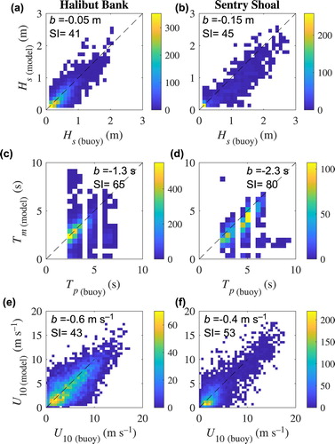
The significant wave height in the model is, on average, biased low relative to measurements. Model performance is slightly better at Halibut Bank than at Sentry Shoal, with bias $b=-0.05\mathrm{m}$ and $b=-0.15\mathrm{m}$, and scatter indices SI = 41 and SI = 45, respectively (Figs 4a and 4b).

A comparison of the modelled and observed wave periods has to consider that the two parameters do not represent the same wave field property. The buoys report the period $T_p$ corresponding to the peak of the wave spectrum. This quantity is inherently noisy and often jumps during the evolution of a multi-modal wave field or at low overall sea states. The model calculates wave period based on different spectral moments (The WAVEWATCH III^® Development Group, 2016). In general, this yields a smoother evolution of the wave period. Here we use the wave period $T_{m02}$, calculated from the 0th ($m_0$) and 2nd ($m_2$) moment, as an estimate for the model wave period $T_m$:(7) $T_m={\left[\overline{f^2}\right]}^{-1/2}={\left[\frac{m_0}{m_2}\right]}^{1/2},$(7) where the overbar denotes a straightforward spectral weighted average and, generally, $T_m<T_p$. This can be seen in the significant negative model bias $b=-1.3\mathrm{s}$ and $b=-2.3\mathrm{s}$ and high scatter indices SI = 65 and SI = 80 for Halibut Bank and Sentry Shoal, respectively (Figs 4c and 4d). The large scatter index is mainly a result of the noisy $T_p$ estimates from the buoy observations, not due to the choice of model output parameter.

Finally, the wind speed input for the wave model is interpolated from the HRDPS wind field onto the model grid. Systematic bias between these wind speeds and the observed wind speeds at the two buoy locations is small (Figs 4e and 4f). However, there is significant scatter, especially for the northern location.

At low sea states the scatter and bias between model and observations are particularly high. Repeating the above analysis but restricting the data to cases in which the modelled wind speed is greater than $5\mathrm{m}{\mathrm{s}}^{-1}$, the following performance parameters are obtained: for the significant wave height, $b=[-0.03,0.2]\mathrm{m}$ and $\mathrm{S}\mathrm{I}=[36,37]$; for the wave period, $b=[-0.3,0.8]\mathrm{s}$ and $\mathrm{S}\mathrm{I}=[31,26]$; and for wind speed, $b=[0.0,0.5]\mathrm{m}{\mathrm{s}}^{-1}$ and $\mathrm{S}\mathrm{I}=[30,32]$, where the first number in the brackets is for Halibut Bank and the second for Sentry Shoal. Thus, for moderate to high wind speeds the model performs significantly better than for low wind speeds. Uncertainties are as expected for coastal wave models (Cavaleri et al., 2018) and agree well with the values reported in Yang et al. (2019) for their wind-wave model of the Salish Sea.

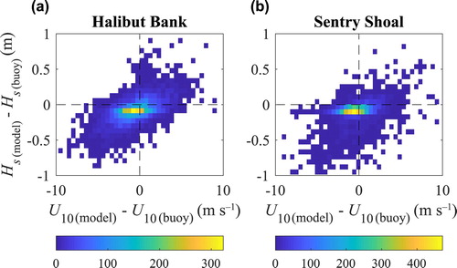
The difference in observed and modelled wave heights can, to a large extent, be related to differences in the wind speeds (Fig. 5). Particularly in enclosed seas, the local winds are affected by a variety of complex but uncertain processes which will feed into the uncertainties of the modelled wind input fields and, thus, result in larger uncertainties in the modelled wave field (see, e.g., Section 2.1. in Cavaleri et al., 2018). Similarly, we find good agreement between modelled and observed wave heights when the wind speed for the model is close to the observed wind speed. Thus, we expect that limitations on accuracy in our wave model predictions are mostly a result of inadequate estimates of wind forcing rather than the physics of ocean wave response.

Fig. 5 Discrepancy of significant wave height $H_s$ between model and observations as a function of wind speed $U_{10}$ discrepancies. Colour indicates data density as counts per cell, given by the colour bars.

c Climatology

1 Winds

Observed winds in the Strait of Georgia are predominantly either northwesterly or southeasterly along the main axis of the Strait, channelled by the mountains that line both sides (Fig. 6). Southeasterlies are generally stronger than northwesterlies, with a significant fraction of them being greater than $10\mathrm{m}{\mathrm{s}}^{-1}$, especially in the central Strait, while northwesterlies are very rarely that strong. Vector mean winds are thus generally northwesterly, albeit with a magnitude of only around $1\mathrm{m}{\mathrm{s}}^{-1}$. The maximum wind speed at Halibut Bank in this two-year period was southeasterly at $17.5\mathrm{m}{\mathrm{s}}^{-1}$ (Fig. 6), but the mean (scalar) wind speed is only $\overline{U_{10}}=4.7\mathrm{m}{\mathrm{s}}^{-1}$. Stations near coasts often show winds speeds less than $5\mathrm{m}{\mathrm{s}}^{-1}$. Such light winds also occur within the Strait, although less frequently. However, even though open water is windier than the coast, winds less than $5\mathrm{m}{\mathrm{s}}^{-1}$ still make up 50% of the record at Halibut Bank (Table 1).

Fig. 6 Wind roses for hourly winds during a 2-year period starting 12 April 2017. The background circles in each rose are 2.5% and 5%.

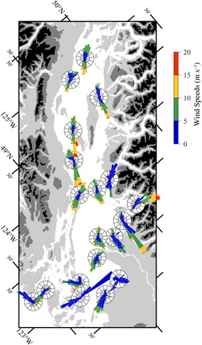
Table 1. Percentage of time in different wind speed and direction conditions at Halibut Bank from April 2017 to April 2019 from the ECCC model output and buoy observations (in parentheses), respectively.

	SE (${90}^{\circ }-{150}^{\circ }$)	SW (${150}^{\circ }-{270}^{\circ }$)	NW (${270}^{\circ }-{330}^{\circ }$)	NE (${330}^{\circ }-{90}^{\circ }$)	Total
(m s^−1)	(%)	(%)	(%)	(%)	(%)
$0-5$	17.7 (13.3)	11.7 (12.0)	21.5 (12.5)	6.2 (12.2)	57.1 (50.0)
$5-10$	15.5 (21.5)	2.2 (5.0)	19.0 (14.8)	0.8 (2.1)	37.2 (43.4)
$>10$	3.6 (4.8)	0.3 (0.6)	1.6 (1.1)	0.2 (0.1)	5.7 (6.6)
Totals	36.5 (39.6)	14.2 (17.6)	42.1 (24.4)	7.2 (14.4)	100 (100)

One exception to this northwest–southeast channelization occurs at the southeastern end of the Strait of Georgia where it meets the flat lands of the Fraser Valley, and significant onshore and offshore winds can occur. Winds at Sand Heads in particular are either southerly (along-strait), northwesterly (i.e., onshore), or easterly (i.e., offshore). Strong easterlies are also seen at Point Atkinson.

A second exception is in Howe Sound, where strong northerly outflow winds occur. Although this is not visible in Fig. 6, the timing of these outflows is not directly linked to the timing of northwesterly or southeasterlies in the Strait of Georgia itself. In addition, they do not coincide with strong easterlies at Point Atkinson.

The model validation discussed in Section 3.b indicates that for a given wind field the model likely provides a good representation of the wave field. Thus, we abandon observed winds and now use the model wind and wave data to describe a quasi-steady wave climate in the Strait of Georgia. In order to understand this wind–wave climate, we will divide model wind conditions into eight different categories based on the model wind speed and wind direction at Halibut Bank (Table 1). Observations are separated into three different magnitudes of wind speed, dividing at boundaries of 5 and $10\mathrm{m}{\mathrm{s}}^{-1}$ (approximately equivalent to significant wave heights at the wave buoys of 0.2 and 1 m, respectively). Winds are then further divided by direction into four categories, two of which are narrowly directional either up- or down-strait (southeasterly or northwesterly, respectively) and two others for which winds are across-strait.

Across-strait wind conditions from the northeast occur mainly in the low wind speed bracket. For both higher wind speed ranges northeasterly winds are found less than $1\text{\%}$ of the time, so these cases are not analyzed in more detail. Instead, for the higher wind speed brackets, we included the analysis of typical outflow wind cases when strong thermally driven winds drain the interior landmass down valleys. At these times, winds in Howe Sound and the Fraser Valley are often high. Here we take northerly winds (${330}^{\circ }-{30}^{\circ }$) in Howe Sound as an indicator of outflow conditions and further partition by wind speed at that location. Because Howe Sound itself is not much more than a few kilometres wide in many areas (i.e., on the order of the grid spacing in the atmospheric model), model winds in this area may be somewhat inaccurate. However, general features of the wind field are probably at least qualitatively reproduced.

In the following, wind and wave parameters in the Strait of Georgia are analyzed for the above stated wind categories, and their spatial distributions are displayed (Figs 7–13). These plots are divided into eight panels, with panels in each row having a common range of wind speeds stated on the left. The columns share a range of wind directions stated at the top, as well as indicated by red arrows. The triangles mark the locations of the two buoys, and the circle indicates the location of the wind data for outflow conditions. The fraction of data that fall within the given wind category is stated on the centre left of each of the three leftmost panels.

Fig. 7 Average wind speed in the Strait of Georgia, as a function of wind direction (columns) and wind speed (rows) at Halibut Bank [(a)–(c), (e)–(g)], and Howe Sound [(d) and (h)]. Top row: moderate Halibut Bank or Howe Sound winds ($5\mathrm{m}{\mathrm{s}}^{-1}\le U_{10}\le 10\mathrm{m}{\mathrm{s}}^{-1}$); bottom row: high Halibut Bank or Howe Sound winds ($U_{10}>10\mathrm{m}{\mathrm{s}}^{-1}$). The red arrows indicate the range of Halibut Bank wind directions in each average. The occurrence rate of the given wind speed and wind direction range at Halibut Bank is stated in the centre left of each of the three leftmost panels. Black arrows are wind vectors, subsampled by a factor of six from the HRDPS model grid.

Fig. 8 Significant wave height $H_s$ in the Strait of Georgia for low wind speeds ($U_{10}<5\mathrm{m}{\mathrm{s}}^{-1}$) at Halibut Bank as a function of wind direction (columns). (a)–(d): mean $H_s$, (e)–(h) 99th percentile of $H_s$. The red arrows indicate the range of wind directions. The occurrence rate of the given wind speed and wind direction range is stated on the centre left of each panel.

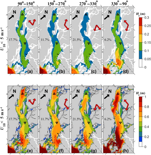
Fig. 9 As in Fig. 7, but showing mean significant wave height $H_s$ in the Strait of Georgia.

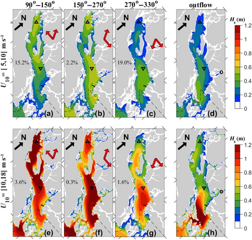
Fig. 10 As in Fig. 7, but showing average of the mean wave period $T_m$ in the Strait of Georgia.

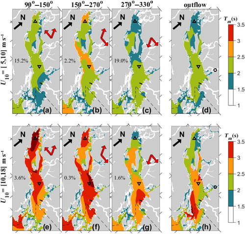
Fig. 11 As in Fig. 7, but showing 99th percentile of significant wave height $H_s$ in the Strait of Georgia.

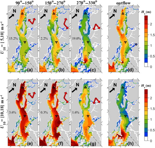
Fig. 12 As in Fig. 7, but showing the average of the mean whitecap coverage γ in the Strait of Georgia.

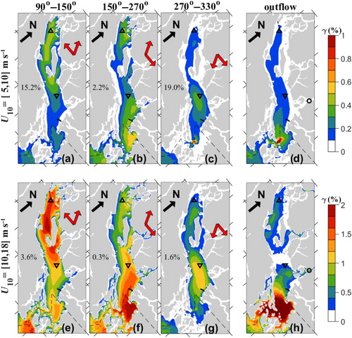
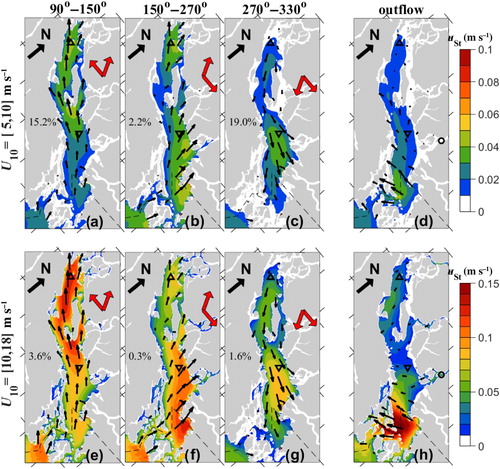
Fig. 13 As in Fig. 7, but showing the average of the mean Stokes drift (wave-induced current) $u_{\mathrm{S}\mathrm{t}}$ in the Strait of Georgia.

At an open coast, the wind speed generally increases with distance downwind from the coastline (Dobson, Perrie, & Toulany, 1989). Here, we find similar behaviour in the Strait of Georgia. Under southeasterly conditions (Figs 7a and 7c), the highest wind speeds are seen north of Halibut Bank. Winds in the southern Strait are only about 70–90% as strong. There is a slight sheltering effect behind the islands in the central Strait and in the northern parts of Malaspina Strait. Winds are also significantly weaker along the Vancouver Island coast south of Denman Island. Under southerly winds (Figs 7b and 7f) the western side of the Strait is even more calm; wind speeds are highest off Sand Heads and in Boundary Bay.

Under northwesterly conditions (Figs 7c and 7g), winds are highest in the central Strait of Georgia, around Halibut Bank. Winds are lower in the northern Strait near Sentry Shoal and in the southern Strait, sheltered behind Gabriola Island as the flow crosses over into the Fraser Valley. Winds are also low in Howe Sound.

Finally, during outflow conditions (Figs 7d and 7h), winds are strongest in the Boundary Bay area at the exit of the Fraser Valley. Strong winds can been seen in Howe Sound and in a tongue extending from the western parts of Howe Sound southwestwards partway across the Strait of Georgia.

2 Waves

Sea states are relatively benign during low wind conditions (speeds $\le 5$ m s${}^{-1}$) at Halibut Bank, which are present most of the time (Table 1). Under these conditions the average significant wave height in the Strait is about 0.1 m (Figs 8a–8d), except in the southern Strait where the average significant wave height reaches about 0.3 m due to outflow winds. However, even in these low wind speed conditions, the extreme values of the significant wave height can be as high as 0.5 m to 1 m (Figs 8e–8h). These rare cases generally occur when the wind speed drops quickly, and the wave field has not yet responded fully.

At higher wind speeds, the significant wave height is usually well correlated with the local wind speed. The largest waves, with heights exceeding 1 m and periods of 4 s are seen in the north for southeasterly winds (Figs 9a and 9e and 10a and 10e), as well as in the central Strait of Georgia for northwesterly winds (Figs 9c and 9g and 10c and 10g). The sheltering effect of islands is quite noticeable, as are the effects of limited fetch, in general, in the northern Strait. Note that although winds themselves are relatively low along the Vancouver Island coast under southwesterly winds (Figs 9b and 9f and 10b and 10f), wave heights are generally quite high.

Under northwesterly winds, wave heights exceed 1.1 m with periods of 3 s north of Sand Heads on the Fraser Delta (Figs 9c and 9g and 10c and 10g) but then decay rapidly to the south and are only 75% as high south of Point Roberts or along the coastlines of the Gulf Islands. Wave heights grow significantly downwind of Halibut Bank reaching their maximum as they propagate onshore on Sturgeon Bank. At highest windspeeds, the 99th percentile of conditions show wave heights of 2.4 m when winds are from the southeast but only 1.5 m when winds are from the north (Figs 11f and 11g).

Finally, although outflow winds are important in Howe Sound and can be much greater than $10\mathrm{m}{\mathrm{s}}^{-1}$ at the entrance to the Sound, the waves in the Sound and the eastern Strait of Georgia are generally small under these conditions. However, on the southwestern side of the Strait, mean significant wave heights are greater than $1.2\mathrm{m}$ ($>0.6\mathrm{m}$) with wave periods greater than $3.5\mathrm{s}$ ($>2.0\mathrm{s}$) for the high wind speed bracket (moderate wind speed bracket) (Figs 9d and 9h and 10d and 10h). During outflow conditions, extreme values of the significant wave heights reach $H_s>2.5\mathrm{m}$ in the southwest corner of the Strait (Fig. 11h), whereas in the central and northern Strait $H_s\ll 1\mathrm{m}$ (Fig. 11h).

The 99th percentile plots also show that large waves can sometimes be seen at the entrance to Discovery Passage under westerly or southerly winds (Figs 11a and 11b), and at Boundary Pass under northwesterly conditions (Fig. 11c). These arise as waves propagate from regions of weak currents into regions of strong opposing tidal currents. The wave action $A=E/\sigma$ is conserved, where E is the wave energy, and σ is the frequency of the waves with respect to the water (Bretherthon & Garrett, 1968). Under opposing currents σ is reduced and wave height increases. A long known but little appreciated consequence is that an opposing current of speed c/4 will completely stop waves with phase speeds c (Garrett & Gemmrich, 2009). Thus, a $1\mathrm{m}{\mathrm{s}}^{-1}$ ($2\mathrm{m}{\mathrm{s}}^{-1}$) current will stop waves of frequencies $f\ge 0.39\mathrm{H}\mathrm{z}$ ($f\ge 0.19\mathrm{H}\mathrm{z}$) (i.e., waves with periods $T\le 2.5\mathrm{s}$ ($T\le 5.1\mathrm{s}$)). Waves at these frequencies are generally seen in the Strait of Georgia (e.g., Fig. 2), and currents of this magnitude are present in these regions. On the other hand, when waves propagate into regions where the flow is in the same direction as wave propagation, wave heights decrease, but these conditions are not shown in our plots.

In none of the cases examined are extraordinarily large waves seen around Sand Heads. The numerical ocean model is known to be deficient in reproducing the large velocities that occur in the outflowing river jet during ebb tides, so the large waves that are observed to occur as the wind sea meets a strong oncoming current are not predicted at this time.

3 Whitecaps

Air–sea gas transfer and the vertical dispersion of oil in the water column is affected by wave breaking, which injects bubbles into the water column and breaks up clumps of oil. Wave breaking also hides the surface expression of internal waves, which are otherwise often visible in the Strait of Georgia and have been the subject of many studies (Shand, 1953; Wang & Pawlowicz, 2011). A parameterization in the WAVEWATCH III^® model can provide an estimate of the percentage of the surface covered by whitecaps. Energy dissipation is largely caused by breaking waves and is related to the fourth moment of the breaking crest length distribution $\mathrm{\Lambda }\left(c\right)$ (Phillips, 1985). Furthermore, the whitecap coverage in deep water is proportional to the second moment of $\mathrm{\Lambda }\left(c\right)$. This relation between wave energy dissipation and whitecap coverage is the basis for the whitecap parameterization in the wave model (Leckler, Ardhuin, Filipot, & Mironov, 2013)

Whitecap percentages are generally low ($\le 0.4\text{\%}$) under moderate winds (Figs 12a–12c). An exception occurs at the southern entrance to the Strait of Georgia, where strong flood tides exiting Boundary Pass interact with northwesterly or outflow winds Figs 12c and 12d) to generate greatly elevated levels of whitecapping. It is likely that similar effects should be seen near Sand Heads, but as discussed earlier, the numerical ocean model does not reproduce the strong currents that, in reality, arise from river outflow at that point.

Under strong northwesterlies the whitecapping percentage rises to more than 1% between Halibut Bank and Sturgeon Bank (Fig. 12g), and under southeasterlies this percentage rises to 1.5% in the northern Strait of Georgia (Fig. 12e). However, the highest percentages (more than 2%) occur in the southern Strait under outflow conditions. These events are associated with the highest wind speeds and large and steep waves resulting in increased wave breaking (Fig. 12h).

4 Stokes drift

The Stokes drift is a residual velocity near the ocean surface that arises from wave orbital motions, in the direction of the wave propagation (van den Bremer & Breivik, 2017). In principle it is not measured by point measurements but leads to a downwind momentum flux and will also cause floating particles to move downwind even without direct wind drag. The Stokes drift is largest at the surface and decays rapidly with depth as orbital motions decrease with depth.

For monochromatic waves the Stokes drift is proportional to the square of the wave steepness, but for a given spectrum of waves the calculations to estimate the Stokes drift term are more complex (van den Bremer & Breivik, 2017). Using a theoretical shape for the wave spectrum known as the Joint North Sea Wave Project (JONSWAP) spectrum (Hasselmann et al., 1973), Webb and Fox-Kemper (2011) calculate that for a saturated wind sea we have(8) $u_{\mathrm{S}\mathrm{t}\mathrm{o}\mathrm{k}\mathrm{e}\mathrm{s}}\approx 0.012U_{10}$(8) for the drift at the surface. This drift rapidly decays with depth. At a reference depth of(9) $z_{\mathrm{r}\mathrm{e}\mathrm{f}\mathrm{e}\mathrm{r}\mathrm{e}\mathrm{n}\mathrm{c}\mathrm{e}}=\frac{c^2}{2g}\approx 0.051\mathrm{m}\times \left(U_{10}/\right(\mathrm{m}{\mathrm{s}}^{-1}){)}^2,$(9) where c is the phase speed for waves at the spectral peak, and we assume $c\approx U_{10}$, the drift is only about 10% of what it is at the surface. At half this depth the drift is 23% of surface values. Thus, for $10\mathrm{m}{\mathrm{s}}^{-1}$ winds, this means that the saturated sea Stokes drift which at the surface is about $12\mathrm{c}\mathrm{m}{\mathrm{s}}^{-1}$ has decreased to less than $3\mathrm{c}\mathrm{m}{\mathrm{s}}^{-1}$ at a depth of 2.5 m and $1\mathrm{c}\mathrm{m}{\mathrm{s}}^{-1}$ at a depth of 5 m.

WAVEWATCH III^® provides an estimate of the surface Stokes drift, calculated from the full wave spectrum (van den Bremer & Breivik, 2017), as a standard output option. The model calculations show that the surface Stokes drift is a few centimetres per second during moderate wind conditions (Figs 13a to 13d), but can reach a maximum of $0.15\mathrm{m}{\mathrm{s}}^{-1}$ when winds are strong and from a southerly direction (Figs 13e and 13f and Fig. 14). Under northeasterly winds this drift is up to $0.1\mathrm{m}{\mathrm{s}}^{-1}$ (Fig. 13g) and would be directly onto Roberts Bank and especially Sturgeon Bank.

Fig. 14 Calculated Stokes drift versus wind speed at Halibut Bank: hourly data and least squares linear fit. Data are divided into $U_{10}\ge 5\mathrm{m}{\mathrm{s}}^{-1}$ (blue crosses, red line) with linear slope m given on each panel, and $U_{10}<5\mathrm{m}{\mathrm{s}}^{-1}$ (grey circles, grey line).

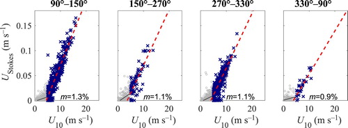
The linear relationship in Eq. (8(8) $u_{\mathrm{S}\mathrm{t}\mathrm{o}\mathrm{k}\mathrm{e}\mathrm{s}}\approx 0.012U_{10}$(8) ) does not describe Stokes drift in the Strait of Georgia. Considering all model data at Halibut Bank with $U_{10}\ge 5\mathrm{m}{\mathrm{s}}^{-1}$ we find instead(10) $u_{\mathrm{S}\mathrm{t}\mathrm{o}\mathrm{k}\mathrm{e}\mathrm{s}}\approx s\times U_{10}-u_{\mathrm{o}\mathrm{f}\mathrm{f}};s=0.011,u_{\mathrm{o}\mathrm{f}\mathrm{f}}=0.04\mathrm{m}{\mathrm{s}}^{-1}$(10) with the Stokes drift approximately zero at lower speeds (Fig. 14). This probably reflects the fact that, on average, the wave field, which is far from saturated, is negligible for wind speeds much lower than $5\mathrm{m}{\mathrm{s}}^{-1}$ (Figs 8a to 8d). Note that the slope of the relationship is not too different from the slope of the relationship in Eq. (8(8) $u_{\mathrm{S}\mathrm{t}\mathrm{o}\mathrm{k}\mathrm{e}\mathrm{s}}\approx 0.012U_{10}$(8) ), but because of the offset term the Stokes drifts in the Strait of Georgia are lower. The relation between wind speed and modelled Stokes drift (Fig. 14) gives a dependence similar to the buoy data, with slightly varying slopes and offsets, depending on the wind direction (Table 2).

Table 2. Linear regression of modelled Stokes drift as a function of wind speed (Eq. (10(10) $u_{\mathrm{S}\mathrm{t}\mathrm{o}\mathrm{k}\mathrm{e}\mathrm{s}}\approx s\times U_{10}-u_{\mathrm{o}\mathrm{f}\mathrm{f}};s=0.011,u_{\mathrm{o}\mathrm{f}\mathrm{f}}=0.04\mathrm{m}{\mathrm{s}}^{-1}$(10) )) for different wind directions.

	SE (${90}^{\circ }-{150}^{\circ }$)	SW (${150}^{\circ }-{270}^{\circ }$)	NW (${270}^{\circ }-{330}^{\circ }$)	NE (${330}^{\circ }-{90}^{\circ }$)
s	0.0129	0.0111	0.0109	0.0086
$u_{\mathrm{o}\mathrm{f}\mathrm{f}}$ ($\mathrm{m}{\mathrm{s}}^{-1}$)	0.0583	0.0410	0.0441	0.0333

The relationship in Eq. (10(10) $u_{\mathrm{S}\mathrm{t}\mathrm{o}\mathrm{k}\mathrm{e}\mathrm{s}}\approx s\times U_{10}-u_{\mathrm{o}\mathrm{f}\mathrm{f}};s=0.011,u_{\mathrm{o}\mathrm{f}\mathrm{f}}=0.04\mathrm{m}{\mathrm{s}}^{-1}$(10) ) is approximately true everywhere in the Strait of Georgia. However, under developing sea conditions, a relationship between the Stokes drift and the wind speed cannot hold universally. Considering model data for the entire Strait, we find for short fetches and for moderate wind speeds that the slope s (Eq. (10(10) $u_{\mathrm{S}\mathrm{t}\mathrm{o}\mathrm{k}\mathrm{e}\mathrm{s}}\approx s\times U_{10}-u_{\mathrm{o}\mathrm{f}\mathrm{f}};s=0.011,u_{\mathrm{o}\mathrm{f}\mathrm{f}}=0.04\mathrm{m}{\mathrm{s}}^{-1}$(10) )) is 0.005 < s < 0.01.

For comparison, note that currents $U_{\mathrm{H}\mathrm{F}}$ in the upper 1 m of the water column measured using an HF radar array in the central Strait of Georgia (Halverson & Pawlowicz, 2016) are(11) $u_{\mathrm{H}\mathrm{F}}\underset{\sim }{<}0.05U_{10}.$(11) The Stokes drift can then be up to 20% of the total current at the surface during high winds, However, the drift is a lower percentage of the current when winds are low. Also, the drift is even smaller for floating objects with a significant drag below the surface.

4 Discussion and conclusions

The Strait of Georgia is often subject to gale warnings and small craft advisories, and experience suggests that the wave conditions can vary significantly from place to place and time to time. A more quantitative understanding of the wave climate is, therefore, necessary for many purposes, and the recent development of a coupled wind–wave–current model for this region, running in a near-real-time mode, as well as the long-term installation of several wave buoys, provides some of the information required to gain such an understanding. The purpose of this study is to evaluate the wave field characteristics in the Strait, not to evaluate model physics or the specific effects of wave–current interactions. The latter would require control runs to test the sensitivity of the results to various parameters, but these have not been carried out.

However, our analysis of two years of wave buoy data first highlights some deficiencies in the currently available observations of wave conditions. In particular, the post-calculated significant wave height at the Sentry Shoal wave buoy is probably too large. This is important at high wind speeds, but (for different reasons) flat calm conditions are also not well identified. Assuming that the available spectral information is correct, both low-frequency cutoff and high-frequency corrections for wave-height calculations using Eq. (2(2) $H_s=4\sqrt{{\int }_{f_0}^{f_1}S\left(f\right)\mathrm{d}f},$(2) ) should be handled in a more sophisticated manner for best results.

Conversely, numerical modelling also has deficiencies because the wind fields provided can be incorrect. Small errors are seen at the buoy locations, but more critical issues may occur with winds in Howe Sound because the topography varies over the scale of the model resolution. However, the wave features for a particular wind seem to be accurately reproduced at the wave buoys and probably over most of the Strait of Georgia.

Not unexpectedly, the wave field in the Strait of Georgia is always fetch limited and limited by the narrowness of the Strait, so that seas are young. Standard parameterizations for significant wave height and other parameters (e.g., Eq. (4(4) $H_s\approx A\frac{U_{10}^2}{g},$(4) )) reproduce relationships reasonably well, but the numerical coefficients in those relationships are often very different than for saturated wind seas. In addition, wave heights and periods undergo significant changes with fetch.

The greatest wave heights occur in the northern Strait of Georgia, during strong southeasterly winds. Although there has been a general tendency for oceanographers to concentrate their attention in the southern Strait, especially in summer, both for logistical reasons and because obvious features, such as the Fraser plume (LeBlond, 1983; Pawlowicz, Di Costanzo, Halverson, Devred, & Johannessen, 2017) require investigation, the northern Strait may be more dynamic—at least for surface waves and possibly for other reasons. An analysis of weather forecasts issued by the Meteorological Service of Canada over the same period as our wave analysis shows that about 30 wind warnings are issued each year for the southern Strait of Georgia compared with 41 for the northern Strait. The majority of these warnings are issued in November, December, and January, averaging about eight (six) per month for the northern (southern) Strait. No advisories were issued in July and August for either area. Thus, winter is clearly the more dynamic period, and the northern Strait is more dynamic than the central and southern Strait.

One important atmospheric phenomenon in this region is the so-called outflow wind. Outflow winds, driven by a combination of katabatic winds and land–sea breeze circulation are very important in setting ocean conditions in Howe Sound (e.g., Bakri, Jackson, & Doherty, 2017), especially in winter (43 wind warnings are issued each year in Howe Sound, averaging eight per month in November, December, and January and none in July or August), but the extent of their importance to the Strait of Georgia has not been known. Our analysis suggests that Howe Sound outflow winds do extend into the Strait but have very little effect on mid-strait significant wave heights although the possible existence of cross-seas and other effects have not been pursued further here. However, it is possible that actual outflow winds in Howe Sound are stronger than those provided by the atmospheric model so that we have underestimated these effects. Outflow conditions in the Fraser Valley, which is wide and, hence, well-resolved in the wind field, lead to very strong winds and large waves (as well as increased whitecapping) in the very southern Strait between Boundary Pass and Point Roberts.

Associated with these large, young waves during outflow conditions are strong wave-induced Stokes drift currents in the southwestern part of the Strait of Georgia reaching, on average, more than $0.15\mathrm{m}{\mathrm{s}}^{-1}$ at the surface. Similar large Stokes drift currents occur in the northern section of the Strait during southerly along-strait winds when the fetch is longest. In the central part of the Strait, waves are even more fetch limited regardless of wind direction. Therefore, the average Stokes drift reaches only approximately $0.1\mathrm{m}{\mathrm{s}}^{-1}$. This is about 20% of the greatest measured speed of wind-driven surface currents in this region (Halverson & Pawlowicz, 2016). Thus, any accurate modelling of the transport of floating material in the Strait will require a correct accounting of the Stokes drift terms. As an example, knowledge of the prevailing wave field will be crucial to understanding the dispersion of potential oil spills. Under calm conditions, oil forms a nearly continuous surface film that will move with the surface currents. However, waves can alter this behaviour, mainly due to the Stokes drift.

An additional effect of waves on oil spills is film break up caused by wave breaking. At higher wind speeds, breaking waves generate turbulent pressure forces that can break up the oil film and generate oil droplets with radii of hundreds of microns, which are then found below the surface (Li & Garrett, 1998). Whitecapping measures the amount of this wave breaking, and one reason for developing a one-way coupled wind–wave–ocean model is to resolve regions where opposing currents can cause increases in wave height, which leads to a steepening of the waves and increased whitecapping.

Our analysis of the model fields shows a correlation between regions of strong current variance and increased whitecapping, suggesting that variable currents are strong enough to be linked to increased wave breaking in the Strait of Georgia. In particular, the regions of strong wave–current interaction, as well as strongly forced waves during outflow conditions, lead to whitecap coverage roughly double that of open ocean conditions under similar wind speeds (Kleiss & Melville, 2010). The 99th percentile plot of significant wave height (Fig. 11) shows that increased wave heights occur in the far northern Strait at the entrance to Discovery Passage and in the far southern Strait near Boundary Pass both are regions where strong and opposing tidal flows can occur and where the variance of the model currents is high. Once subducted, vertical velocities of up to $0.7\mathrm{m}{\mathrm{s}}^{-1}$ have been found to subduct bubbles to depths of more than 160 m in Boundary Pass (Baschek & Farmer, 2010), and presumably this would occur with oil droplets in that area as well.

The modelled wave fields, however, do not show any increase near Sand Heads, which is notorious for the presence of large waves during ebb tides when the river jets out into the Strait of Georgia. This is probably because the numerical ocean model does not reproduce these strong outflow jets. Further improvements in the ocean model in this region are then necessary to evaluate conditions at Sand Heads.

Acknowledgments

We especially thank Doug Latornell (UBC) for implementing the routine forecasts as part of the SalishSeaNowcast automation. We also thank C. Yu (Meteorological Service of Canada) for providing statistics on forecast wind warnings.

Disclosure statement

No potential conflict of interest was reported by the author(s).

Additional information

Funding

The development of the Salish Sea wave forecast has been supported by funds from Ocean Networks Canada (ONC), Fisheries and Oceans Canada (DFO), and the Marine Environmental Observation, Prediction and Response (MEOPAR) network's Observation Core. The data analysis received funding from Metro Vancouver and MEOPAR.

References

- Ardhuin, F., Rogers, W. E., Babanin, A., Filipot, J.-F., Magne, R., Roland, A., … Collard, F. (2010). Semi-empirical dissipation source functions for ocean waves: Part I, definitions, calibration and validations. Journal of Physical Oceanography, 40, 1917–1941. doi: 10.1175/2010JPO4324.1
- Bakri, T., Jackson, P., & Doherty, F. (2017). Along-channel winds in Howe Sound: Climatological analysis and case studies. Atmosphere-Ocean, 55(1), 12–30. doi:10.1080/07055900.2016.1233094
- Baschek, B., & Farmer, D. M. (2010). Gas bubbles as oceanographic tracers. Journal of Atmospheric and Oceanic Technology, 27(1), 241–245. doi: 10.1175/2009JTECHO688.1
- Battjes, J. A., Zitman, T. J., & Holthuijsen, L. H. (1987). A reanalysis of the spectra observed in JONSWAP. Journal of Physical Oceanography, 17(8), 1288–1295. doi: 10.1175/1520-0485(1987)017<1288:AROTSO>2.0.CO;2
- Bretherthon, F. P., & Garrett, C. J. R. (1968). Wave trains in inhomogeneous moving media. Proceedings of the Royal Society of London A, 302, 529–554. doi: 10.1098/rspa.1968.0034
- Cavaleri, L., Abdalla, S., Benetazzo, A., Bertotti, L., Bidlot, J., Breivik, O., … van der Westhuysen, A. J. (2018). Wave modelling in coastal and inner seas. Progress in Oceanography, 167, 164–233. doi:10.1016/j.pocean.2018.03.010
- Dobson, F., Perrie, W., & Toulany, B. (1989). On the deep-water fetchlaws for wind-generated surface gravity waves. Atmosphere-Ocean, 27, 210–236. doi:10.1080/07055900.1989.9649334
- Farazmand, M., & Sapsis, T. (2019). Surface waves enhance particle dispersion. Fluids, 4, 55. doi:10.3390/fluids4010055
- Garrett, C., & Gemmrich, J. (2009). Rogue waves. Physics Today, 62(6), 62–63. doi: 10.1063/1.3156339
- Gemmrich, J., & Garrett, C. (2011). Dynamical and statistical explanations of observed occurrence rates of rogue waves. Natural Hazards and Earth System Science, 11, 1437–1446. doi:10.5194/nhess-11-1437-2011
- Halverson, M., & Pawlowicz, R. (2016). Tide, wind, and river forcing of the surface currents in the Fraser River plume. Atmosphere-Ocean, 54(2), 131–152. doi: 10.1080/07055900.2016.1138927
- Halverson, M., Pawlowicz, R., & Chavanne, C. (2017). Dependence of 25-MHz HF radar working range on near-surface conductivity, sea state, and tides. Journal of Atmospheric and Oceanic Technology, 34(2), 447–462. doi: 10.1175/JTECH-D-16-0139.1
- Hasselmann, K., Barnett, T. P., Bouws, E., Carlson, H., Cartwright, D. E., Enke, K., … Walden, H. (1973). Measurements of wind-wave growth and swell decay during the Joint North Sea Wave Project (JONSWAP). Dt. Hydrogr. Zeitschrift, Ergänzungsheft 12, 1–95.
- Hill, P. R., & Davidson, S. H. (2002). Preliminary modelling of sediment transport on the upper foreslope of the Fraser River delta. (Current Research 2002-E2). Ottawa: Natural Resources Canada, Geological Survey of Canada.
- Holthuijsen, L. H. (2007). Waves in oceanic and coastal waters. New York: Cambridge University Press.
- Janssen, P. (2004). The interaction of ocean waves and wind. Cambridge, UK: Cambridge University Press.
- Janssen, T. T., & Herbers, T. H. C. (2009). Nonlinear wave statistics in a focal zone. Journal of Physical Oceanography, 39(8), 1948–1964. doi:10.1175/2009JPO4124.1
- Kastner, S. E., Horner-Devine, A. R., & Thomson, J. (2018). The influence of wind and waves on spreading and mixing in the Fraser River plume. Journal of Geophysical Research: Oceans, 129(3), 6818–6840. doi:10.1029/2018JC013765
- Kleiss, J. M., & Melville, W. K. (2010). Observations of wave breaking kinematics in fetch-limited seas. Journal of Physical Oceanography, 40, 2575–2604. doi: 10.1175/2010JPO4383.1
- Large, W. G., & Pond, S. (1981). Open ocean momentum flux measurements in moderate to strong winds. Journal of Physical Oceanography, 11(3), 324–336. doi: 10.1175/1520-0485(1981)011<0324:OOMFMI>2.0.CO;2
- LeBlond, P. H. (1983). The Strait of Georgia: Functional anatomy of a coastal sea. Canadian Journal of Fisheries and Aquatic Sciences, 40(7), 1033–1063. doi: 10.1139/f83-128
- Leckler, F., Ardhuin, F., Filipot, J.-F., & Mironov, A. (2013). Dissipation source terms and whitecap statistics. Ocean Modelling, 70, 62–74. doi: 10.1016/j.ocemod.2013.03.007
- Li, M., & Garrett, C. (1998). The relationship between oil droplet size and upper ocean turbulence. Marine Pollution Bulletin, 36, 961–970. doi: 10.1016/S0025-326X(98)00096-4
- Milbrandt, J. A., Bélair, S., Faucher, M., Vallée, M., Carrera, M. L., & Glazer, A. (2016). The pan-Canadian High Resolution (2.5 km) Deterministic Prediction System. Weather and Forecasting, 31, 1791–1816. doi:10.1175/WAF-D-16-0035.1
- NCEP (2016). ETOPOI global relief model. Retrieved from https://www.ngdc.noaa.gov/mgg/global/global.html
- Pawlowicz, R., Beardsley, R., Lentz, S., Dever, E., & Anis, A. (2001). The air–sea toolbox: Boundary-layer parameterization for everyone. Eos, Transactions American Geophysical Union, 84(1), 2. doi: 10.1029/01EO00004
- Pawlowicz, R., Di Costanzo, R., Halverson, M., Devred, E., & Johannessen, S. (2017). Advection, surface area, and sediment load of the Fraser River plume under variable wind and river forcing. Atmosphere-Ocean, 55(4-5), 293–313. doi: 10.1080/07055900.2017.1389689
- Pettersson, H., Kahma, K. K., & Tuomi, L. (2010). Wave directions in a narrow bay. Journal of Physical Oceanography, 40, 155–169. doi:10.1175/2009JPO4220.1
- Phillips, O. M. (1985). Spectral and statistical properties of the equilibrium range in wind-generated gravity waves. Journal of Fluid Mechanics, 156, 505–531. doi: 10.1017/S0022112085002221
- Shand, J. A. (1953). Internal waves in Georgia Strait. Eos, Transactions American Geophysical Union, 34(6), 849–856. doi: 10.1029/TR034i006p00849
- Soontiens, N., & Allen, S. (2017). Modelling sensitivities to mixing and advection in a sill-basin estuarine system. Ocean Modelling, 112, 17–32. doi:10.1016/j.ocemod.2017.02.008
- Soontiens, N., Allen, S., Latornell, D., Le Souef, K., Machuca, I., Paquin, J.-P., … Korabel, V. (2016). Storm surges in the Strait of Georgia simulated with a regional model. Atmosphere-Ocean, 54, 1–21. doi:10.1080/07055900.2015.1108899
- The WAVEWATCH III® Development Group. (2016). User manual and system documentation of WAVEWATCH III® version 5.16 (NOAA/NWS/NCEP/MMAB Tech. Note, 329), College Park, MD, USA. Retrieved from http://polar.ncep.novaa.gov/waves/wavwwatch/manaul.v5.16.pdf.
- Transportation Safety Board of Canada. (2003). Marine investigation report, capsizing and loss of life, small fishing vessel Cap Rouge II: Off entrance to Fraser River, British Columbia (Report M02W0147). Retrieved from http://www.bst-tsb.gc.ca/eng/rapports-reports/marine/2002/m02w0147/m02w0147.html
- van den Bremer, T. S., & Breivik, Ø. (2017). Stokes drift. Philosophical Transactions of the Royal Society A: Mathematical, Physical and Engineering Sciences, 376, 20170104. doi:10.1098/rsta.2017.0104
- Wang, C., & Pawlowicz, R. (2011). Propagation speeds of strongly nonlinear near–surface internal waves in the Strait of Georgia. Journal of Geophysical Research: Oceans, 116(C10021). doi:10.10.1029/2010JC006776
- Webb, A., & Fox-Kemper, B. (2011). Wave spectral moments and Stokes drift estimation. Ocean Modelling, 40, 273–288. doi: 10.1016/j.ocemod.2011.08.007
- Yang, Z., Garcia-Medina, G., Wu, W.-C., Wang, T., & Mauger, G. (2019). Modeling analysis of the swell and wind-sea climate in the Salish Sea. Estuarine, Coastal and Shelf Science, 224, 289–300. doi:10.1016/j.ecss.2019.04.043