Classification of Clustered Snow Off Dates Over British Columbia, Canada, from Mean Sea Level Pressure

ABSTRACT

Atmosphere–ocean teleconnections influence the accumulation and melt of snow in western Canada and can be useful in seasonal forecasting of snowmelt and runoff. Interannual variation in these atmosphere–ocean modes has been shown to influence the accumulation and melt of snow within British Columbia (BC), Canada. We investigate fall mean sea level pressure (MSLP) globally as a predictor of remotely sensed snowmelt dates within BC. We use the last day of continuous snow cover ($S{D}_{\mathrm{o}\mathrm{f}\mathrm{f}}$) detected from time series satellite imagery acquired by the Moderate Resolution Imaging Spectroradiometer for the hydrological years 2000–2018. It has been shown that $S{D}_{\mathrm{o}\mathrm{f}\mathrm{f}}$ is correlated with continuous snow duration and is also of interest to seasonal forecasters. Global MSLP from the Fifth major global reanalysis produced by the European Centre for Medium-range Weather Forecasts was obtained over hydrological years 1979–2018. An S-mode (time versus location) principal component analysis was carried out on both datasets. The $S{D}_{\mathrm{o}\mathrm{f}\mathrm{f}}$ principal component scores were grouped using a k-means clustering routine. Using evolutionary feature selection, the subset of MSLP principal components that provided good linear discrimination of the $S{D}_{\mathrm{o}\mathrm{f}\mathrm{f}}$ clusters were found. We explore the atmospheric MSLP principal components that influence the timing of snowmelt over BC and use them to predict the $S{D}_{\mathrm{o}\mathrm{f}\mathrm{f}}$ clusters at a seasonal lead time.

Résumé

[Traduit par la rédaction] La présente étude expose les attributs spatiaux et temporels de quelque 45 millions d’éclairs nuage-sol détectés par le Réseau canadien de détection de la foudre entre 1999 et 2018. Même si les mises à niveau des capteurs ont amélioré l’efficacité de la détection et la précision d’emplacement des éclairs nuage-sol, les structures spatiales à grande échelle demeurent à peu près les mêmes que celles d’une étude antérieure couvrant la période 1999-2008. Les analyses, utilisant des cellules de surface uniforme de 10 km de côté, décrivent les caractéristiques régionales et saisonnières des éclairs négatifs et positifs, le pourcentage et la densité d’éclairs des éclairs positifs, ainsi que les courants de pointe des premières décharges pour les deux polarités. L’activité de la foudre au-dessus des provinces et des territoires connaît un pic au cours de l’été, allant de 95,9 % à 76,8 % de l’activité annuelle dans les Territoires-du-Nord-Ouest et l’Ontario, respectivement. En hiver, les éclairs sont rares, survenant généralement dans l’extrême sud de l’Ontario et dans les provinces atlantiques, et au-dessus des zones extracôtières à l’ouest de l’île de Vancouver et des eaux côtières longeant la Nouvelle-Écosse. Une analyse préliminaire donne à penser que, comparativement à la période 1999-2008, la majorité de l’ouest canadien et du nord du Canada ont observé plus de journées avec foudre au cours de la période 2009-2018, tandis que l’est du Canada en a enregistré moins. Une analyste statistique réalisée auprès de 154 stations dans l’ensemble du Canada a révélé que les hausses décennales (baisses) enregistrées dans 5 (31) stations étaient appréciables, atteignant au moins un niveau de confiance de 90 %, dont 4 (16) étaient significatives avec un niveau de confiance de 95 %.

KEYWORDS:

• British Columbia
• Canada
• MODIS
• snow cover timing
• reanalysis
• sea level pressure
• time series

1 Introduction

In western Canada spatial and annual variation in winter precipitation patterns are highly dependent on synoptic-scale circulation patterns that influence the formation and trajectory of winter storms off the North Pacific Ocean. Global scale atmosphere–ocean modes, or teleconnections, have been shown to influence the frequency of these different synoptic-scale circulation types over British Columbia (BC) and western Canada (Stahl et al., 2006).

The primary atmosphere–ocean interactions that have been shown to influence winter precipitation in western Canada are the El Niño Southern Oscillation (ENSO), Pacific Decadal Oscillation (PDO), Pacific–North America (PNA) pattern, and Arctic Oscillation (AO). Previous studies have related variation in these climate modes to variation in the climate over BC, including temperature and precipitation (e.g., Mantua et al., 1997; Shabbar & Khandekar, 1996), as wll as the timing and duration of snow cover (e.g., Bevington et al., 2019; Moore & McKendry, 1996).

The Moderate Resolution Imaging Spectroradiometer (MODIS) satellite sensor images the world four times daily as a result of the ascending and descending overpasses of the MODIS Terra and MODIS Aqua platforms. Using MODIS-derived snow cover, Bevington et al. (2019) derived the start ($\mathrm{S}{\mathrm{D}}_{\mathrm{o}\mathrm{n}}$) and end ($\mathrm{S}{\mathrm{D}}_{\mathrm{o}\mathrm{f}\mathrm{f}}$) dates of continuous snow coverage over BC and related these metrics to both the ENSO and PDO. Results from that study revealed strong correlations with both ENSO and the PDO, particularly with the $\mathrm{S}{\mathrm{D}}_{\mathrm{o}\mathrm{f}\mathrm{f}}$ and duration ($\mathrm{S}{\mathrm{D}}_{\mathrm{d}\mathrm{u}\mathrm{r}}$), and found that the strength of the correlations varied regionally throughout BC and are influenced by elevation. Because the timing and duration of snow cover has important economic, social, and ecological implications for BC, the ability to predict these fields at a seasonal lead time would be of great benefit.

Despite strong links between these atmosphere–ocean modes and snow cover, some variation in snow cover over BC is likely to be described by variation in the atmosphere not captured by teleconnection indices alone, such as has been shown for streamflow response in Colorado (Regonda et al., 2006). Global mean sea level pressure (MSLP) reanalysis datasets provide the opportunity to determine which global atmospheric patterns influence snow cover in BC. Many studies have shown that low-frequency variability in global MSLP demonstrates gradually evolving modes closely linked to the ENSO phenomenon, and this slow evolution of the atmosphere provides the opportunity for long-range predictive skill exploited by many statistical models based on these atmospheric quantities (Latif et al., 1998).

The objective of this study is to test the suitability of global MSLP averaged during the fall to better understand and predict spatial patterns and variation in $\mathrm{S}{\mathrm{D}}_{\mathrm{o}\mathrm{f}\mathrm{f}}$ annually within BC.

2 Study area and data

a Study Area

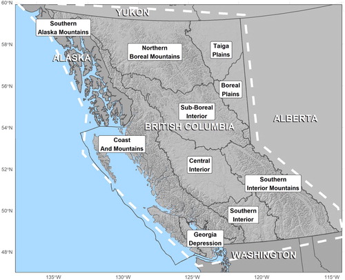
Our study area, shown in Fig. 1, includes BC with small inclusions of southeastern Alaska and a 100 km buffer into neighbouring jurisdictions because many watersheds extend just beyond provincial borders. This is the maximum extent of the Bevington et al. (2019) data. In order to describe the spatial variation in $\mathrm{S}{\mathrm{D}}_{\mathrm{o}\mathrm{f}\mathrm{f}}$ with consistency, BC Eco-provinces are referenced in the subsequent sections and are labelled in Fig. 1 (Ministry of Environment and Climate Change Strategy, 2011).

Fig. 1 The study area (white dashed line), which extends just beyond the border of British Columbia and includes the panhandle of Alaska. The British Columbia Eco-province regions are labelled.

b MODIS Snow Cover

The MODIS sensor is a multispectral optical imaging sensor aboard both the Aqua and Terra satellites that provides important observations of land, atmospheric, and oceanic processes globally. With 36 spectral bands varying in resolution from 250 to 1000 m and a combined daily repeat interval, MODIS is well equipped for monitoring changes over time (since late 1999) across broad geographic areas. A number of derivative products are available from MODIS Collection 6 (C6), including the daily snow cover datasets from Terra (MOD10A1; Hall & Riggs, 2016a) and Aqua (MYD10A1; Hall & Riggs, 2016b), which are based on the normalized difference snow index (NDSI) derived from MODIS Level 1B calibrated radiance (Riggs et al., 2016). In Bevington et al. (2019), these data were used to determine the $\mathrm{S}{\mathrm{D}}_{\mathrm{o}\mathrm{n}}$, $\mathrm{S}{\mathrm{D}}_{\mathrm{o}\mathrm{f}\mathrm{f}}$, and $\mathrm{S}{\mathrm{D}}_{\mathrm{d}\mathrm{u}\mathrm{r}}$ of continuous snow cover over the study area and to quantify their response to ENSO and the PDO regionally. The code and gridded output of this work is available online at (https://github.com/bcgov/ts-rs-modis-snow); in addition, the years 2000, 2001, and 2018 were processed for this study. In this analysis we only use annual $\mathrm{S}{\mathrm{D}}_{\mathrm{o}\mathrm{f}\mathrm{f}}$ dates, which are in units of days-since-1-September (DSS). We decided to apply $\mathrm{S}{\mathrm{D}}_{\mathrm{o}\mathrm{f}\mathrm{f}}$ in this study because the $\mathrm{S}{\mathrm{D}}_{\mathrm{o}\mathrm{f}\mathrm{f}}$ date is a known indicator of winter–spring runoff and influences spring–summer soil moisture content (Cohen, 1994). In addition, $\mathrm{S}{\mathrm{D}}_{\mathrm{o}\mathrm{f}\mathrm{f}}$ is a driver of northern vegetation phenology which has wide-ranging influences, for example, the migration patterns of ungulates (John et al., 2020).

c European Centre for Medium-range Weather Forecasts ERA5

The Fifth major global reanalysis (ERA5) produced by the European Centre for Medium-range Weather Forecasts (ECMWF) is a global data product with a resolution of 31 km and 137 atmosphere levels from the earth's surface up to a height of 80 km (Hersbach et al., 2019). For the ERA5 MSLP field, data are assimilated from a combination of land-, ship-, and buoy-based pressure observations operated by the World Meteorological Organization-Information System (WIS). The ERA5 reanalysis data are available hourly or monthly. For this study we used the monthly MSLP product for predicting $\mathrm{S}{\mathrm{D}}_{\mathrm{o}\mathrm{f}\mathrm{f}}$ from ECMWF (2020). The assimilation and physical processing for ERA5 is carried out by the ECMWF's Integrated Forecast System (IFS). The monthly MSLP data were obtained for the years 1979–2018.

3 Methods

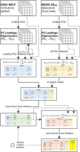
The processing workflow applied in this study is illustrated by Fig. 2. Principal component analysis (PCA) was applied to both the gridded annual $\mathrm{S}{\mathrm{D}}_{\mathrm{o}\mathrm{f}\mathrm{f}}$ data from Bevington et al. (2019) and the ERA5 monthly MSLP data averaged over the fall (September–November). All the principal component (PC) scores derived from the $\mathrm{S}{\mathrm{D}}_{\mathrm{o}\mathrm{f}\mathrm{f}}$ time series were then used as inputs into a k-means cluster analysis. Decomposition of the ${\mathrm{S}\mathrm{D}}_{\mathrm{o}\mathrm{f}\mathrm{f}}$ time series was only necessary for computational efficiency and repeatability of the k-means cluster analysis; the spatial loadings are presented in Appendix A (Figs A1–A5). The leading PC scores from the MSLP time series served as candidate predictors in linear discriminant analysis (LDA) in which the $\mathrm{S}{\mathrm{D}}_{\mathrm{o}\mathrm{f}\mathrm{f}}$ k-means cluster results defined groups. Using the leave-one-out cross-validated (LOOCV) overall accuracy as a cost metric, feature selection for predictive LDA was carried out using an evolutionary approach. For the subset LDA, standardized coefficients were related back to the spatially reconstructed MSLP loadings to help infer atmospheric mechanisms contributing to the discrimination of the $\mathrm{S}{\mathrm{D}}_{\mathrm{o}\mathrm{f}\mathrm{f}}$ clusters.

Fig. 2 Workflow diagram for predicting clustered $\mathrm{S}{\mathrm{D}}_{\mathrm{o}\mathrm{f}\mathrm{f}}$ from ERA5 mean sea level pressure.

a k-Means Cluster Analysis of Annual $\mathrm{S}{\mathrm{D}}_{\mathrm{o}\mathrm{f}\mathrm{f}}$

1 Principal component analysis

Decomposition of the MODIS-derived annual $\mathrm{S}{\mathrm{D}}_{\mathrm{o}\mathrm{f}\mathrm{f}}$ dates over BC was performed using PCA before applying a k-means cluster analysis in order to allow efficient computation. The type of PCA applied was in the form of S-Mode (time versus location) outlined in Richman (1986), because this type of decomposition has been extensively used in the field of atmospheric science and similar disciplines for studying major modes of temporal variation in spatially distributed attribute fields, such as time series of MSLP (Demšar et al., 2012). In S-Mode PCA, features represent locations (pixels), while observations correspond to repeated measures (years) (Fig. 2). Before applying the PCA, for each location (pixel), fall MSLP data (September–November, see Section 3.b) was first zero-centred by subtracting the 1979–2018 climatological mean from each observation and then scaled to have unit variance by dividing by the standard deviation. An unrotated PCA solution for both MSLP and $\mathrm{S}{\mathrm{D}}_{\mathrm{o}\mathrm{f}\mathrm{f}}$ was computed using the R programming language “stats” package (R Core Team, 2019).

2 k-means cluster analysis

The $\mathrm{S}{\mathrm{D}}_{\mathrm{o}\mathrm{f}\mathrm{f}}$ PC scores were used as inputs into a non-hierarchical k-means clustering routine. Cluster analysis is by nature an exploratory analysis technique, and there are many different clustering methods available (Gotelli & Ellison, 2013). The k-means is one of the most frequently used clustering methods in the environmental sciences, and an efficient version detailed in Hartigan and Wong (1979) was used in this study. The k-means clustering routine is an iterative method that begins by partitioning the data into k groups, forming k initial group centres. The algorithm seeks to then find a k-partition of the data with a locally optimal within-cluster sum of squares by moving observations from one cluster to another based on their dissimilarity score, typically Euclidean distance; (Hartigan & Wong, 1979). Various methods exist for determining the number of k-clusters to use; in this study silhouette plots were used to determine an appropriate number of clusters given the ${\mathrm{S}\mathrm{D}}_{\mathrm{o}\mathrm{f}\mathrm{f}}$ data. Silhouette values represent how similar an observation is to its assigned cluster compared with other clusters based on multivariate distance and provide a graphical means for determining cluster appropriateness (Rousseeuw, 1987).

b Decomposition of Fall Mean Sea Level Pressure

The monthly data from the ERA5 MSLP were averaged over the fall (September–November) preceding the snow accumulation period at each location (pixel) for a given year, referred to here as $\mathrm{M}\mathrm{S}\mathrm{L}{\mathrm{P}}_{\mathrm{F}\mathrm{A}\mathrm{L}\mathrm{L}}$. The $\mathrm{M}\mathrm{S}\mathrm{L}{\mathrm{P}}_{\mathrm{F}\mathrm{A}\mathrm{L}\mathrm{L}}$ was calculated for each year over the 1979–2018 period. The $\mathrm{M}\mathrm{S}\mathrm{L}{\mathrm{P}}_{\mathrm{F}\mathrm{A}\mathrm{L}\mathrm{L}}$ time series was transformed though decomposition using methods outlined in Section 3.a.1. Common to S-Mode PCA analysis is the visual interpretation of the spatially reconstructed eigenvectors for each of the retained PCs (Demšar et al., 2012). The $\mathrm{M}\mathrm{S}\mathrm{L}{\mathrm{P}}_{\mathrm{F}\mathrm{A}\mathrm{L}\mathrm{L}}$ eigenvectors, also referred to as loadings, were spatially reconstructed in this way to aid in the interpretation of potential underlying physical mechanisms associated with a given $\mathrm{M}\mathrm{S}\mathrm{L}{\mathrm{P}}_{\mathrm{F}\mathrm{A}\mathrm{L}\mathrm{L}}$ PC.

c Linear Discriminant Analysis

There ares multiple origins for LDA, both Fisher (1936) and Mahalanobis (1936/2018) developed different approaches to discriminating between groups. There is, however, a mathematical relationship between Fisher's linear discriminant functions (LDF) and the classification functions defined by Mahalanobis (e.g., Kshirsagar & Arseven, 1975). Unlike cluster analysis, discriminant analysis assigns samples to groups or classes. Intuitively LDA is similar to PCA in that they both decompose the data to fewer dimensions. Where PCA is seeking to generate a new axis that maximizes the variation within the data, LDA seeks to generate a new axis that maximizes the separation between established categories and is, therefore, supervised. Mathematically, a linear combination of the original variables can be represented by Eq. (1), (1) $Z_i=a_{i1}{Y}_1+a_{i2}{Y}_2+\dots +a_{in}{Y}_n.$(1) Assuming the multivariate means $\overline{\mathbf{Y}}$ vary among groups, the goal of LDA is to find $a$ in Eq. (1) that maximizes the among-group sum of squares for a given set of $Z_i$ (Gotelli & Ellison, 2013). Fisher's approach proceeds by performing an eigen analysis of ${\mathbf{W}}^{-1}\mathbf{B}$, where $\mathbf{B}$ is the between-group sum of squares cross-products (SSCP) matrix and $\mathbf{W}$ is the within-group SSCP matrix. Ordered by the resulting eigenvalues, the corresponding eigenvectors $a_i$ are the coefficients in Eq. (1), also referred to as canonical discriminant function coefficients, or loadings. When the data are standardized, these loadings indicate which of the discriminating variables are most important in differentiating between the groups. Classification can be performed by minimizing the Mahalanobis distance among observations within groups adjusted for the prior probabilities when they are not equal (Venables & Ripley, 2002). In this study, the $\mathrm{M}\mathrm{S}\mathrm{L}{\mathrm{P}}_{\mathrm{F}\mathrm{A}\mathrm{L}\mathrm{L}}$ PCs constituted the possible predictor variables, and the $\mathrm{S}{\mathrm{D}}_{\mathrm{o}\mathrm{f}\mathrm{f}}$ k-means clusters served as factors to be classified. Proportional priors were assumed, and LDA was computed using the R programming language MASS package (Venables & Ripley, 2002).

d Evolution Feature Selection

A genetic algorithm (GA) is a stochastic optimization and search algorithm inspired by biological evolution and natural selection (Mitchell, 1998). A typical application of binary GAs in statistical modelling is subset selection (Scrucca, 2013). Feature selection is a natural extension of GAs using a binary string indicating the presence or absence of a predictor from a given candidate subset. The fitness of a candidate subset is usually represented by one of several model selection criteria, such as the Akaike information criterion (AIC) or the Bayesian information criterion (BIC), in the case of regression (Bozdogan, 2003). With the retained $\mathrm{M}\mathrm{S}\mathrm{L}{\mathrm{P}}_{\mathrm{F}\mathrm{A}\mathrm{L}\mathrm{L}}$ PCs defining the predictor set and the $\mathrm{S}{\mathrm{D}}_{\mathrm{o}\mathrm{f}\mathrm{f}}$ clusters as the response variable, the subset of PCs that maximized the LOOCV overall accuracy from a predictive LDA was found using a GA algorithm, applying principles described in Scrucca (2013). Specifically, the fitness of a candidate subset was defined as the LOOCV accuracy, where accuracy is determined through resampling. In the case that more than one model had the same LOOCV accuracy, the ratio of the distance between group means to the total variance of each group, in addition to the number of inputs were considered in identifying the most parsimonious model. Generations were continued so that the population mean fitness appeared to become asymptotic, suggesting no more gain in model fitness would be achieved through additional generations.

4 Results

a Annual $\mathrm{S}{\mathrm{D}}_{\mathrm{o}\mathrm{f}\mathrm{f}}$ Date Decomposition

Principal component analysis of the annual MODIS-derived $\mathrm{S}{\mathrm{D}}_{\mathrm{o}\mathrm{f}\mathrm{f}}$ time series data was applied before cluster analysis to improve computational efficiency and repeatability of the k-means clustering. All the resulting PC scores were used as input to k-means cluster analysis. The corresponding $\mathrm{S}{\mathrm{D}}_{\mathrm{o}\mathrm{f}\mathrm{f}}$ spatial loadings are available in Appendix A and lend insight into the major modes of $\mathrm{S}{\mathrm{D}}_{\mathrm{o}\mathrm{f}\mathrm{f}}$ variation over BC.

b k-Means $\mathrm{S}{\mathrm{D}}_{\mathrm{o}\mathrm{f}\mathrm{f}}$ Clusters

A k-means cluster analysis was carried out on the PC scores from the PCA of the $\mathrm{S}{\mathrm{D}}_{\mathrm{o}\mathrm{f}\mathrm{f}}$ time series. Using k equal to 2, 3, and 4 clusters, silhouette plots were generated to help determine the most appropriate number of clusters given the $\mathrm{S}{\mathrm{D}}_{\mathrm{o}\mathrm{f}\mathrm{f}}$ data. These results are illustrated in Fig. 3. Based on the silhouette scores, it was determined that k = 2 clusters was the most appropriate number of clusters and had the greatest average silhouette width (Fig. 3a). Table 1 shows the $\mathrm{S}{\mathrm{D}}_{\mathrm{o}\mathrm{f}\mathrm{f}}$ annual time series cluster results for k = 2 clusters.

Fig. 3 Silhouette plots corresponding to k-clusters for the $S{D}_{\mathrm{o}\mathrm{f}\mathrm{f}}$ time series data for 2–4 clusters (x-axis); the red line indicates the average silhouette score.

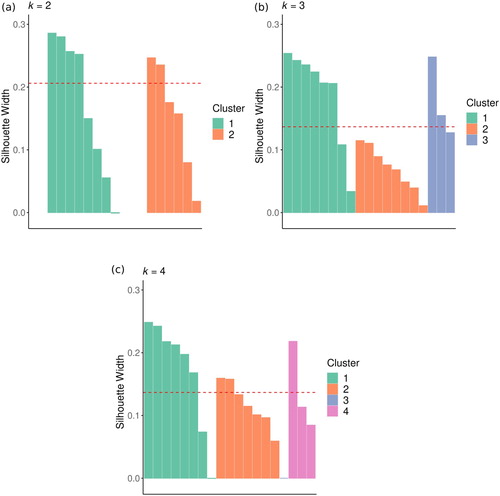
Table 1. The $\mathrm{S}{\mathrm{D}}_{\mathrm{o}\mathrm{f}\mathrm{f}}$ time series cluster value from k-means cluster analysis with k = 2 for each hydrologic year over the 2000–2018 period.

Year	2000	2001	2002	2003	2004	2005	2006	2007	2008	2009
Cluster	1	1	2	2	2	1	1	1	1	2
Year	2010	2011	2012	2013	2014	2015	2016	2017	2018
Cluster	1	1	1	1	2	2	2	2	2

From the clustered $\mathrm{S}{\mathrm{D}}_{\mathrm{o}\mathrm{f}\mathrm{f}}$ time series shown in Table 1 the average $\mathrm{S}{\mathrm{D}}_{\mathrm{o}\mathrm{f}\mathrm{f}}$ was calculated over the years corresponding to each cluster, as well as over the entire time series. Each $\mathrm{S}{\mathrm{D}}_{\mathrm{o}\mathrm{f}\mathrm{f}}$ cluster average is displayed in Fig. 4 as the difference from the $\mathrm{S}{\mathrm{D}}_{\mathrm{o}\mathrm{f}\mathrm{f}}$ time series mean. In addition, the difference between the Cluster 1 and Cluster 2 means is shown.

Fig. 4 Difference of $\mathrm{S}{\mathrm{D}}_{\mathrm{o}\mathrm{f}\mathrm{f}}$ by cluster from the time series average $\mathrm{S}{\mathrm{D}}_{\mathrm{o}\mathrm{f}\mathrm{f}}$: (a) (2000–2018), and (d) difference between (b) Cluster 1 mean and (c) Cluster 2 mean $\mathrm{S}{\mathrm{D}}_{\mathrm{o}\mathrm{f}\mathrm{f}}$. See Table 1 for corresponding cluster years.

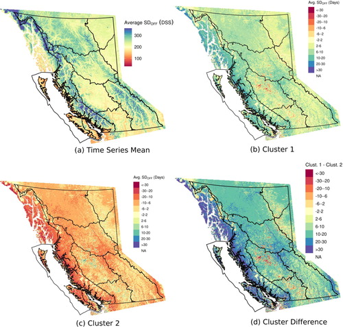
The mapped clusters shown in Fig. 4 indicate that mean $\mathrm{S}{\mathrm{D}}_{\mathrm{o}\mathrm{f}\mathrm{f}}$ over Cluster 1 years is generally later than the mean $\mathrm{S}{\mathrm{D}}_{\mathrm{o}\mathrm{f}\mathrm{f}}$ over the entire time series (Fig. 4b), while mean $\mathrm{S}{\mathrm{D}}_{\mathrm{o}\mathrm{f}\mathrm{f}}$ over Cluster 2 years is generally earlier than mean $\mathrm{S}{\mathrm{D}}_{\mathrm{o}\mathrm{f}\mathrm{f}}$ over the entire time series (Fig. 4c). This suggests that the clusters have classified the $\mathrm{S}{\mathrm{D}}_{\mathrm{o}\mathrm{f}\mathrm{f}}$ time series into early and late years relative to the time series mean $\mathrm{S}{\mathrm{D}}_{\mathrm{o}\mathrm{f}\mathrm{f}}$. The difference between the clusters, represented in Fig. 4d as Cluster 1 minus Cluster 2, reveals important spatial patterns. A median $\mathrm{S}{\mathrm{D}}_{\mathrm{o}\mathrm{f}\mathrm{f}}$ difference of 14 days with an interquartile range of 11 days is observed in Fig. 4d. It appears that the largest differences in $\mathrm{S}{\mathrm{D}}_{\mathrm{o}\mathrm{f}\mathrm{f}}$ of around 15–30 days between Cluster 1 and Cluster 2 years occur along the Coast and Mountains, southern Alaskan, and Georgia Depression regions. The northwest Central Interior and southwest Southern Interior Mountains regions also reveal relatively large differences in $\mathrm{S}{\mathrm{D}}_{\mathrm{o}\mathrm{f}\mathrm{f}}$ between cluster years. Differences in $\mathrm{S}{\mathrm{D}}_{\mathrm{o}\mathrm{f}\mathrm{f}}$ for Cluster 1 and Cluster 2 years appear less pronounced within some areas of the Taiga and Boreal Plains and Southern Interior Mountains regions.

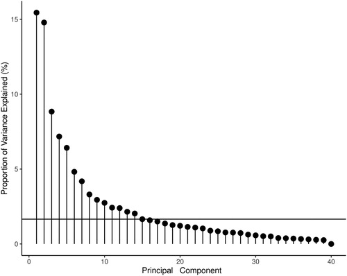
c Fall Mean Sea Level Pressure Decomposition

The total variance explained by each PC derived from PCA of the $\mathrm{M}\mathrm{S}\mathrm{L}{\mathrm{P}}_{\mathrm{F}\mathrm{A}\mathrm{L}\mathrm{L}}$ time series (1979–2018) is shown in Fig. 5. Based on this plot, the leading 15 PCs were retained and represent the candidate inputs for LDA feature selection. The first 15 PCs explain 81% of the total $\mathrm{M}\mathrm{S}\mathrm{L}{\mathrm{P}}_{\mathrm{F}\mathrm{A}\mathrm{L}\mathrm{L}}$ variance.

Fig. 5 Proportion of variance explained for each of the eigenvectors from principal component analysis of $\mathrm{M}\mathrm{S}\mathrm{L}{\mathrm{P}}_{\mathrm{F}\mathrm{A}\mathrm{L}\mathrm{L}}$ time series over the 1979–2018 period. The horizontal line indicates the percentage of total variance explained by the 15th PC (1.7%); PCs below this were not retained for feature selection.

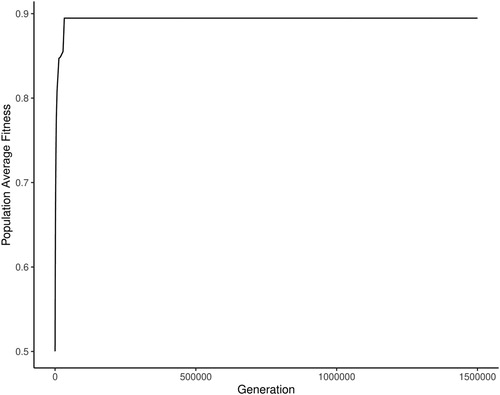
d Evolutionary Feature Selection

The leading PCs described in Section 4.c comprised the set of candidate predictors for predictive LDA of the $\mathrm{S}{\mathrm{D}}_{\mathrm{o}\mathrm{f}\mathrm{f}}$ clusters. Using principles described in Mitchell (1998) the subset of $\mathrm{M}\mathrm{S}\mathrm{L}{\mathrm{P}}_{\mathrm{F}\mathrm{A}\mathrm{L}\mathrm{L}}$ PC inputs that maximized the LOOCV accuracy of the LDA classifier were identified. With an initial population of 2000 randomly initialized candidate subsets, the initial population was evolved over a total of 1,500,000 generations. The population mean LOOCV with each generation is plotted in Fig. 6. The absence of change seen in generations beyond 500,000 suggests an optimal subset of features for classifying the ${\mathrm{S}\mathrm{D}}_{\mathrm{o}\mathrm{f}\mathrm{f}}$ clusters was likely identified. There were several candidate feature subsets that obtained an LOOCV accuracy of 0.89, which was the maximum observed accuracy of any subset. However, the subset including $\mathrm{M}\mathrm{S}\mathrm{L}{\mathrm{P}}_{\mathrm{F}\mathrm{A}\mathrm{L}\mathrm{L}}$ PC1, PC2, PC3, PC8, PC10, and PC11 had a high degree of separation with respect to the first discriminant function (LD1), but significantly fewer inputs than some of the other models with marginally greater separation and was chosen as the best feature subset. The loadings for the subset of $\mathrm{M}\mathrm{S}\mathrm{L}{\mathrm{P}}_{\mathrm{F}\mathrm{A}\mathrm{L}\mathrm{L}}$ PCs selected for LDA are represented spatially in Appendix B (Figs B1 and B2).

Fig. 6 Mean population fitness (LOOCV accuracy) of LDA classifier over 1500000 consecutive generations for an initial population size of 2000 randomly assigned $\mathrm{M}\mathrm{S}\mathrm{L}{\mathrm{P}}_{\mathrm{F}\mathrm{A}\mathrm{L}\mathrm{L}}$ PC candidate feature subsets.

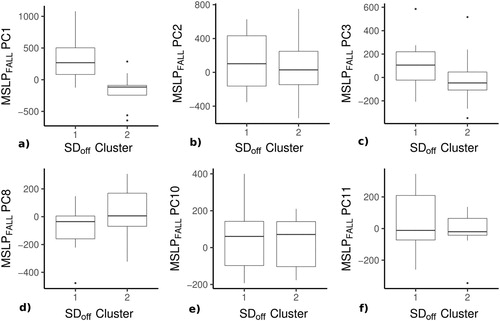
e Linear Discriminant Analysis

The subset of $\mathrm{M}\mathrm{S}\mathrm{L}{\mathrm{P}}_{\mathrm{F}\mathrm{A}\mathrm{L}\mathrm{L}}$ PCs described in Section 4.d were used as input to LDA for predicting the $\mathrm{S}{\mathrm{D}}_{\mathrm{o}\mathrm{f}\mathrm{f}}$ clusters. The $\mathrm{M}\mathrm{S}\mathrm{L}{\mathrm{P}}_{\mathrm{F}\mathrm{A}\mathrm{L}\mathrm{L}}$ PCs are shown in Fig. 7 by $\mathrm{S}{\mathrm{D}}_{\mathrm{o}\mathrm{f}\mathrm{f}}$ cluster showing the relative separation each PC provides. From these plots, we see that the $\mathrm{M}\mathrm{S}\mathrm{L}{\mathrm{P}}_{\mathrm{F}\mathrm{A}\mathrm{L}\mathrm{L}}$ PC1 seems to provide the most definitive separation of the $\mathrm{S}{\mathrm{D}}_{\mathrm{o}\mathrm{f}\mathrm{f}}$ clusters.

Fig. 7 Boxplots showing the distribution of each $\mathrm{M}\mathrm{S}\mathrm{L}{\mathrm{P}}_{\mathrm{F}\mathrm{A}\mathrm{L}\mathrm{L}}$ PC score selected for LDA by $\mathrm{S}{\mathrm{D}}_{\mathrm{o}\mathrm{f}\mathrm{f}}$ cluster.

The linear discriminant coefficients and function scores are summarized in the following sections.

1 Discriminant function coefficients

The LD1 provides a linear transformation of the $\mathrm{M}\mathrm{S}\mathrm{L}{\mathrm{P}}_{\mathrm{F}\mathrm{A}\mathrm{L}\mathrm{L}}$ subset of PCs into one dimension that has maximal separation between $\mathrm{S}{\mathrm{D}}_{\mathrm{o}\mathrm{f}\mathrm{f}}$ group means. This linear transformation is defined by the coefficients $a_i$ in Eq. (1). The original LD1 coefficients are shown in Table 2, and the standardized coefficients (loadings) are shown in Fig. 8. The standardized loadings can be used to determine which of the PC inputs are most important in discriminating between the $\mathrm{S}{\mathrm{D}}_{\mathrm{o}\mathrm{f}\mathrm{f}}$ clusters. Coefficients close to the origin (zero) have less influence on LD1 than those with coefficients larger (in absolute value) than zero.

Fig. 8 Standardized loadings (coefficients) for the first linear discriminant function (LD1). Coefficients shown are for the subset of $\mathrm{M}\mathrm{S}\mathrm{L}{\mathrm{P}}_{\mathrm{F}\mathrm{A}\mathrm{L}\mathrm{L}}$ PCs.

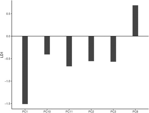
Table 2. Discriminant function coefficients (loadings) for first (and only) linear discriminant function (LD1).

	PC1	PC2	PC3	PC8	PC10	PC11
LD1 Coefficient	−0.00369	−0.00152	−0.00232	0.00350	−0.00254	−0.00402

The standardized loadings shown in Fig. 8 suggest that LD1 is contrasting PC1, PC2, PC3, PC10, and PC11, which all have negative standardized coefficients, with PC8, which has a positive coefficient. Based on the magnitude of the standardized coefficients, we find that $\mathrm{M}\mathrm{S}\mathrm{L}{\mathrm{P}}_{\mathrm{F}\mathrm{A}\mathrm{L}\mathrm{L}}$ PC1 has the greatest influence on LD1, while PC10 has the least.

2 Discriminant function scores

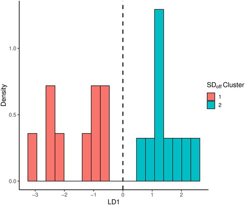
We use a scatterplot of the two $\mathrm{S}{\mathrm{D}}_{\mathrm{o}\mathrm{f}\mathrm{f}}$ clusters projected onto the dimension of the LD1 discriminant solution to assess the separation of the $\mathrm{S}{\mathrm{D}}_{\mathrm{o}\mathrm{f}\mathrm{f}}$ clusters (Fig. 9). From this plot it appears that observations with LD1 scores less than zero indicate $\mathrm{S}{\mathrm{D}}_{\mathrm{o}\mathrm{f}\mathrm{f}}$ Cluster 1 years, while LD1 scores greater than zero appear to correspond to $\mathrm{S}{\mathrm{D}}_{\mathrm{o}\mathrm{f}\mathrm{f}}$ Cluster 2. Therefore, LD1 provides good separation of the two $\mathrm{S}{\mathrm{D}}_{\mathrm{o}\mathrm{f}\mathrm{f}}$ clusters, but the greatest uncertainty occurs for LD1 scores close to the mean of zero, where the probability densities slightly overlap.

Fig. 9 Distribution of LD1 scores by ${\mathrm{S}\mathrm{D}}_{\mathrm{o}\mathrm{f}\mathrm{f}}$ cluster. The dashed line indicates the LD1 mean.

3 Leave-one-out cross-validated classification accuracy

With a total of 19 observations, the predictive LDA obtained a LOOCV accuracy of 0.89%, misidentifying two of the observations (Table 3). Year 2001 was classified as a Cluster 2 year when in fact it was a Cluster 1 year. Year 2014 was classified as a Cluster 1 year when it was actually a Cluster 2 year.

Table 3. The leave-one-out cross validated confusion matrix for predictive LDA clasification of the $\mathrm{S}{\mathrm{D}}_{\mathrm{o}\mathrm{f}\mathrm{f}}$ clusters.

	Classified
True Cluster	Cluster 1	Cluster 2	Total
Cluster 1	9	1	10
Cluster 2	1	8	9

For both 2001 and 2014 it is worth noting that neutral ENSO conditions occurred leading up to and during the $\mathrm{M}\mathrm{S}\mathrm{L}{\mathrm{P}}_{\mathrm{F}\mathrm{A}\mathrm{L}\mathrm{L}}$ period based on the Oceanic Niño Index (ONI) index (Huang et al., 2017). This possibly explains why the LD1 scores for these years were close to the mean and inaccurately classified.

5 Discussion

a ERA5 Mean Sea Level Pressure and ${\mathrm{S}\mathrm{D}}_{\mathrm{o}\mathrm{f}\mathrm{f}}$

The standardized LDA coefficients reveal which of the $\mathrm{M}\mathrm{S}\mathrm{L}{\mathrm{P}}_{\mathrm{F}\mathrm{A}\mathrm{L}\mathrm{L}}$ PCs are most influential on the classification of the $\mathrm{S}{\mathrm{D}}_{\mathrm{o}\mathrm{f}\mathrm{f}}$ clusters (Fig. 8). The $\mathrm{M}\mathrm{S}\mathrm{L}{\mathrm{P}}_{\mathrm{F}\mathrm{A}\mathrm{L}\mathrm{L}}$ PC1 has the greatest influence on LD1 because it has the largest (in absolute value) standardized coefficient; it also explains the most variation in the $\mathrm{M}\mathrm{S}\mathrm{L}{\mathrm{P}}_{\mathrm{F}\mathrm{A}\mathrm{L}\mathrm{L}}$ time series (Fig. 5). The negative LD1 coefficient indicates that as $\mathrm{M}\mathrm{S}\mathrm{L}{\mathrm{P}}_{\mathrm{F}\mathrm{A}\mathrm{L}\mathrm{L}}$ PC1 increases LD1 decreases. This means that larger positive PC1 scores are associated with Cluster 1 or a relatively late $\mathrm{S}{\mathrm{D}}_{\mathrm{o}\mathrm{f}\mathrm{f}}$ over BC, while larger negative PC1 scores are associated with Cluster 2 (i.e., a relatively early $\mathrm{S}{\mathrm{D}}_{\mathrm{o}\mathrm{f}\mathrm{f}}$ over BC, see Fig. 9). The spatial loading pattern for $\mathrm{M}\mathrm{S}\mathrm{L}{\mathrm{P}}_{\mathrm{F}\mathrm{A}\mathrm{L}\mathrm{L}}$ PC1 displays strong negative loadings centred over Oceania and Southeast Asia, while strong positive loadings occur off the western coast of equatorial South America and the central Pacific Ocean (Fig. B1a). Variation in $\mathrm{M}\mathrm{S}\mathrm{L}{\mathrm{P}}_{\mathrm{F}\mathrm{A}\mathrm{L}\mathrm{L}}$ at these centres is associated with the Walker circulation, which is closely linked with ENSO (Horel & Wallace, 1981). A common metric of ENSO is the Southern Oscillation Index (SOI), which is the difference in MSLP between Darwin, Australia, and Tahiti (Trenberth, 1976). The $\mathrm{M}\mathrm{S}\mathrm{L}{\mathrm{P}}_{\mathrm{F}\mathrm{A}\mathrm{L}\mathrm{L}}$ PC1 has strong positive loadings over Tahiti and negative loadings over Darwin and is significantly correlated with the SOI ($\rho =0.92,p<0.0001$) and ONI ($\rho =-0.89,p<0.0001$). This suggests that when $\mathrm{M}\mathrm{S}\mathrm{L}{\mathrm{P}}_{\mathrm{F}\mathrm{A}\mathrm{L}\mathrm{L}}$ is negative, the trade winds over the tropical Pacific weaken, leading to a countercurrent that results in abnormally warm surface sea temperatures in the region. This drives enhanced upper tropospheric divergence in the tropics and convergence in the subtropics, and over western Canada this manifests as the familiar positive PNA pattern (Horel & Wallace, 1981), which has a significant influence on winter climate over western Canada (Shabbar, 2006). Interestingly, PC1 is also significantly correlated ($\rho =0.35;p=0.0279$) with the Antarctic Oscillation index (AAO) and the PDO ($\rho =-0.65,p<0.0001$); however, the physical mechanisms driving these relationships are unclear.

The $\mathrm{M}\mathrm{S}\mathrm{L}{\mathrm{P}}_{\mathrm{F}\mathrm{A}\mathrm{L}\mathrm{L}}$ PC2 has a negative standardized coefficient with LD1 (Fig. 8). The spatial loadings for PC2 reveal strong positive loadings throughout Antarctica, while negative loadings occur in the sub-polar regions over the Southern Ocean (Fig. B1b). The loadings for the $\mathrm{M}\mathrm{S}\mathrm{L}{\mathrm{P}}_{\mathrm{F}\mathrm{A}\mathrm{L}\mathrm{L}}$ PC2 indicate a similar pattern to that of the southern hemisphere annular mode described in Thompson and Wallace (2000) and is significantly correlated ($\rho =-0.88,p<0.0001$) with the AAO. The loadings also reveal strong negative centres over James Bay up to Gulf of Alaska. When $\mathrm{M}\mathrm{S}\mathrm{L}{\mathrm{P}}_{\mathrm{F}\mathrm{A}\mathrm{L}\mathrm{L}}$ increases over this region, assuming the pattern persists, it is likely that the polar jet stream is diverted by this high pressure, resulting in drier and warmer winter conditions over much of BC (Shabbar, 2006). This might explain why positive LD1 values, and earlier $\mathrm{S}{\mathrm{D}}_{\mathrm{o}\mathrm{f}\mathrm{f}}$, are associated with negative PC2 scores.

Similar to the $\mathrm{M}\mathrm{S}\mathrm{L}{\mathrm{P}}_{\mathrm{F}\mathrm{A}\mathrm{L}\mathrm{L}}$ PC2, PC3 appears to be contrasting the polar high with the subpolar lows, however, in the northern hemisphere (Fig. B1c). There are widespread negative loadings corresponding spatially with the northern polar high. Positive loading occurs at the subpolar low south of Alaska and over much of the Pacific and Oceania. This pattern is consistent with the the general loading pattern of the northern hemisphere annular mode (Thompson & Wallace, 2000), and the $\mathrm{M}\mathrm{S}\mathrm{L}{\mathrm{P}}_{\mathrm{F}\mathrm{A}\mathrm{L}\mathrm{L}}$ PC3 is indeed correlated ($\rho =0.63,p<0.0001$) with the AO. Although the $\mathrm{M}\mathrm{S}\mathrm{L}{\mathrm{P}}_{\mathrm{F}\mathrm{A}\mathrm{L}\mathrm{L}}$ PC3 does have negative loadings over much of Canada, it also has strong positive loadings centred over the Aleutian Low. Assuming that $\mathrm{M}\mathrm{S}\mathrm{L}{\mathrm{P}}_{\mathrm{F}\mathrm{A}\mathrm{L}\mathrm{L}}$ is indicative of winter patterns, this suggests that, when PC3 is positive, the Aleutian Low weakens and likely permits the flow of moist air off the Pacific to be directed away from the Gulf of Alaska and into BC, with increased winter precipitation leading to later $\mathrm{S}{\mathrm{D}}_{\mathrm{o}\mathrm{f}\mathrm{f}}$ (negative LD1 score).

The $\mathrm{M}\mathrm{S}\mathrm{L}{\mathrm{P}}_{\mathrm{F}\mathrm{A}\mathrm{L}\mathrm{L}}$ PC8 is the only PC with a positive LD1 coefficient (Fig. 8). Similar to the $\mathrm{M}\mathrm{S}\mathrm{L}{\mathrm{P}}_{\mathrm{F}\mathrm{A}\mathrm{L}\mathrm{L}}$ PC3, positive loadings are observed centred over the Aleutian Low, with negative loadings over much of western Canada (Fig. B1d). However, the negative loadings of the $\mathrm{M}\mathrm{S}\mathrm{L}{\mathrm{P}}_{\mathrm{F}\mathrm{A}\mathrm{L}\mathrm{L}}$ PC8 are more pronounced over western Canada and Alaska. This indicates that PC8 may capture the $\mathrm{M}\mathrm{S}\mathrm{L}{\mathrm{P}}_{\mathrm{F}\mathrm{A}\mathrm{L}\mathrm{L}}$ pressure over the Canadian High. The positive standardized LD1 coefficient indicates that as $\mathrm{M}\mathrm{S}\mathrm{L}{\mathrm{P}}_{\mathrm{F}\mathrm{A}\mathrm{L}\mathrm{L}}$ increases over western Canada, Alaska, and the North Pacific, mean $\mathrm{S}{\mathrm{D}}_{\mathrm{o}\mathrm{f}\mathrm{f}}$ over BC tends to occur later. The enhanced high pressure in this region is associated with the persistence of cold Arctic air and could explain the later $\mathrm{S}{\mathrm{D}}_{\mathrm{o}\mathrm{f}\mathrm{f}}$ dates. The $\mathrm{M}\mathrm{S}\mathrm{L}{\mathrm{P}}_{\mathrm{F}\mathrm{A}\mathrm{L}\mathrm{L}}$ PC8 has no significant correlation with any established atmosphere–ocean indices (i.e., ONI, SOI, AAO, AO, NAO, PNA, or PDO).

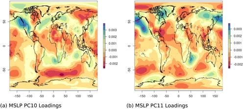
For $\mathrm{M}\mathrm{S}\mathrm{L}{\mathrm{P}}_{\mathrm{F}\mathrm{A}\mathrm{L}\mathrm{L}}$ PC10, positive loadings are seen over much of western BC (Fig. B2a). The negative LD1 coefficient implies that as $\mathrm{M}\mathrm{S}\mathrm{L}{\mathrm{P}}_{\mathrm{F}\mathrm{A}\mathrm{L}\mathrm{L}}$ PC10 increases $\mathrm{S}{\mathrm{D}}_{\mathrm{o}\mathrm{f}\mathrm{f}}$ tends to occur later; $\mathrm{M}\mathrm{S}\mathrm{L}{\mathrm{P}}_{\mathrm{F}\mathrm{A}\mathrm{L}\mathrm{L}}$ PC10 appears to capture variation along the Coast and Mountains region of BC, where differences in $\mathrm{S}{\mathrm{D}}_{\mathrm{o}\mathrm{f}\mathrm{f}}$ between Cluster 1 and Cluster 2 years are large. This is likely because when $\mathrm{M}\mathrm{S}\mathrm{L}{\mathrm{P}}_{\mathrm{F}\mathrm{A}\mathrm{L}\mathrm{L}}$ PC10 is negative, a pronounced low pressure system is located over western BC, which would result in enhanced winter precipitation in the region assuming the pattern persists into the winter months. The $\mathrm{M}\mathrm{S}\mathrm{L}{\mathrm{P}}_{\mathrm{F}\mathrm{A}\mathrm{L}\mathrm{L}}$ PC10 appears to have the least influence on LD1 (Fig. 8).

The $\mathrm{M}\mathrm{S}\mathrm{L}{\mathrm{P}}_{\mathrm{F}\mathrm{A}\mathrm{L}\mathrm{L}}$ PC11 has the most influence on LD1 other than PC1 but only slightly more influence than the other PCs (Fig. 8). The loadings for PC11 show strong positive coefficients with two main centres over the north Pacific Aleutian Islands and off the coast of California (Fig. B2b). There are strong negative coefficients located over the southeast United States and north of Alaska, as well as moderate negative loading over much of western North America. The negative LD1 coefficient implies that when $\mathrm{M}\mathrm{S}\mathrm{L}{\mathrm{P}}_{\mathrm{F}\mathrm{A}\mathrm{L}\mathrm{L}}$ is high over western North America, $\mathrm{S}{\mathrm{D}}_{\mathrm{o}\mathrm{f}\mathrm{f}}$ is earlier than average, and when it is high over the North Pacific, $\mathrm{S}{\mathrm{D}}_{\mathrm{o}\mathrm{f}\mathrm{f}}$ is later than average. With higher pressure present over western North America, advection of dry continental air towards BC may be enhanced, causing warmer drier conditions over BC and earlier $\mathrm{S}{\mathrm{D}}_{\mathrm{o}\mathrm{f}\mathrm{f}}$ dates. The $\mathrm{M}\mathrm{S}\mathrm{L}{\mathrm{P}}_{\mathrm{F}\mathrm{A}\mathrm{L}\mathrm{L}}$ PC11 also appears to be negatively correlated ($\rho =-0.39,p=0.0133$) with the PNA pattern, which has been shown to have an important influence on snow accumulation and melt over BC (Moore & McKendry, 1996).

b Uncertainties

Although this study has demonstrated that PCs of $\mathrm{M}\mathrm{S}\mathrm{L}{\mathrm{P}}_{\mathrm{F}\mathrm{A}\mathrm{L}\mathrm{L}}$ can discriminate between clustered patterns of $\mathrm{S}{\mathrm{D}}_{\mathrm{o}\mathrm{f}\mathrm{f}}$ over BC, the following uncertainties remain. These include the robustness of these signals over time. While indices such as ONI evolve at a rate that allows for an annual mean signature, some of the more regionally specific $\mathrm{M}\mathrm{S}\mathrm{L}{\mathrm{P}}_{\mathrm{F}\mathrm{A}\mathrm{L}\mathrm{L}}$ PCs may change more rapidly. This suggests that changing the aggregation period from the fall could have a significant impact on the results. Many of the proposed mechanisms in the study assume that the $\mathrm{M}\mathrm{S}\mathrm{L}{\mathrm{P}}_{\mathrm{F}\mathrm{A}\mathrm{L}\mathrm{L}}$ patterns persist into winter and spring to some degree; however, this persistence may not always occur. In addition, it is common to use field weighting of geophysical data to achieve grid-area parity (Chung & Nigam, 1999). No weighting of $\mathrm{M}\mathrm{S}\mathrm{L}{\mathrm{P}}_{\mathrm{F}\mathrm{A}\mathrm{L}\mathrm{L}}$ was applied in this study and, as a result, variability at the poles is likely exaggerated. Finally, while LOOCV was used to establish the out-of-sample accuracy of the predictive LDA, a longer time series would allow for a more robust validation of the overall classification accuracy of the $\mathrm{S}{\mathrm{D}}_{\mathrm{o}\mathrm{f}\mathrm{f}}$ clusters.

c Implications

The cluster analysis of $\mathrm{S}{\mathrm{D}}_{\mathrm{o}\mathrm{f}\mathrm{f}}$ essentially split the $\mathrm{S}{\mathrm{D}}_{\mathrm{o}\mathrm{f}\mathrm{f}}$ time series into “early” and “late” years relative to the time series mean (Fig. 4). At locations where the difference between these $\mathrm{S}{\mathrm{D}}_{\mathrm{o}\mathrm{f}\mathrm{f}}$ clusters is large, there is likely to be significant variation in phenology and hydrology that correspond to the timing of $\mathrm{S}{\mathrm{D}}_{\mathrm{o}\mathrm{f}\mathrm{f}}$. The results in this study show that specific PCs of $\mathrm{M}\mathrm{S}\mathrm{L}{\mathrm{P}}_{\mathrm{F}\mathrm{A}\mathrm{L}\mathrm{L}}$ can be used to discriminate between clusters of remotely sensed $\mathrm{S}{\mathrm{D}}_{\mathrm{o}\mathrm{f}\mathrm{f}}$ over the previous 19 years when input into an LDA classifier. The spatial loadings for the subset of $\mathrm{M}\mathrm{S}\mathrm{L}{\mathrm{P}}_{\mathrm{F}\mathrm{A}\mathrm{L}\mathrm{L}}$ PCs help provide insight into some plausible atmospheric mechanisms that explain the ability of each $\mathrm{M}\mathrm{S}\mathrm{L}{\mathrm{P}}_{\mathrm{F}\mathrm{A}\mathrm{L}\mathrm{L}}$ PC to discriminate between the $\mathrm{S}{\mathrm{D}}_{\mathrm{o}\mathrm{f}\mathrm{f}}$ clusters over BC. As future satellite data become available we will be able to more adequately validate the relationships demonstrated in this study.

6 Conclusions

We used MODIS-derived 500 m gridded $\mathrm{S}{\mathrm{D}}_{\mathrm{o}\mathrm{f}\mathrm{f}}$ over BC as input into a k-means cluster analysis resulting in two $\mathrm{S}{\mathrm{D}}_{\mathrm{o}\mathrm{f}\mathrm{f}}$ clusters representing early and late conditions relative to the time series mean $\mathrm{S}{\mathrm{D}}_{\mathrm{o}\mathrm{f}\mathrm{f}}$ (2000–2018). We aggregated global ERA5 MSLP over the fall ($\mathrm{M}\mathrm{S}\mathrm{L}{\mathrm{P}}_{\mathrm{F}\mathrm{A}\mathrm{L}\mathrm{L}}$) annually for the 1979–2018 period. Principal component analysis in S-Mode (time versus location) was applied to the $\mathrm{M}\mathrm{S}\mathrm{L}{\mathrm{P}}_{\mathrm{F}\mathrm{A}\mathrm{L}\mathrm{L}}$ time series, and the resulting PC scores were joined with the $\mathrm{S}{\mathrm{D}}_{\mathrm{o}\mathrm{f}\mathrm{f}}$ clusters by year. Using an evolutionary approach, the subset of $\mathrm{M}\mathrm{S}\mathrm{L}{\mathrm{P}}_{\mathrm{F}\mathrm{A}\mathrm{L}\mathrm{L}}$ PCs that maximized the LOOCV classification accuracy of the $\mathrm{S}{\mathrm{D}}_{\mathrm{o}\mathrm{f}\mathrm{f}}$ clusters were identified using an LDA. For the subset LDA model, an overall predictive LOOCV accuracy of 0.89 was observed, suggesting good discrimination of the $\mathrm{S}{\mathrm{D}}_{\mathrm{o}\mathrm{f}\mathrm{f}}$ clusters over the time series. The standardized linear discriminant function coefficients were plotted and related to the spatially reconstructed $\mathrm{M}\mathrm{S}\mathrm{L}{\mathrm{P}}_{\mathrm{F}\mathrm{A}\mathrm{L}\mathrm{L}}$ eigenvectors or loadings. This comparison allowed us to define the relationship between the subset $\mathrm{M}\mathrm{S}\mathrm{L}{\mathrm{P}}_{\mathrm{F}\mathrm{A}\mathrm{L}\mathrm{L}}$ loading patterns and atmosphere–ocean modes known to influence the winter climate of western Canada, such as ENSO. However, the $\mathrm{M}\mathrm{S}\mathrm{L}{\mathrm{P}}_{\mathrm{F}\mathrm{A}\mathrm{L}\mathrm{L}}$ PCs do not represent a standard index of these atmospheric phenomena. Generally, we find that the $\mathrm{S}{\mathrm{D}}_{\mathrm{o}\mathrm{f}\mathrm{f}}$ clusters are sensitive to major variation in the atmosphere, as the leading three $\mathrm{M}\mathrm{S}\mathrm{L}{\mathrm{P}}_{\mathrm{F}\mathrm{A}\mathrm{L}\mathrm{L}}$ PCs, closely related to ENSO, as well as the southern and northern annular modes, respectively, were included in the subset LDA. However, several PCs capturing more subtle $\mathrm{M}\mathrm{S}\mathrm{L}{\mathrm{P}}_{\mathrm{F}\mathrm{A}\mathrm{L}\mathrm{L}}$ variation influencing $\mathrm{S}{\mathrm{D}}_{\mathrm{o}\mathrm{f}\mathrm{f}}$ were also included in the subset LDA. In locations where the difference in $\mathrm{S}{\mathrm{D}}_{\mathrm{o}\mathrm{f}\mathrm{f}}$ between clusters is significant this study could have important implications for disciplines where the timing of snow melt is an important forcing, such as the timing of spring freshet and peak flows.

The overall framework of our findings is not likely to change as the dense time series of gridded snow cover data continues. The Visible Infrared Imaging Radiometer Suite (VIIRS) satellite sensor provides continuity from the MODIS imagery and will allow for further investigation of snow cover over time. In addition, dense time series of high-resolution satellite imagery being collected by new satellite constellations by private sector companies, such as Planet, may allow for high-resolution studies of time series gridded snow cover data.

Acknowledgements

The authors are very grateful to Michael Allchin, Stephen Déry, Yuexian Wang, John Rex, and William MacKenzie for conversations that helped inform the early direction of this work. The authors thank the reviewers for their valuable guidance provided in response to this work. Also, we acknowledge the open data science community, specifically free access to the British Columbia River Forecast Centre, ERA5, MODIS, Google Earth Engine, R, Python, and QGIS.

Disclosure statement

No potential conflict of interest was reported by the author(s).

Additional information

Funding

This research was supported by the British Columbia Ministry of Forests, Lands, Natural Resource Operations and Rural Development [grant number R&S-28]; Natural Sciences and Engineering Research Council of Canada [grant number 518294].

Appendix A

$\mathrm{S}{\mathrm{D}}_{\mathrm{o}\mathrm{f}\mathrm{f}}$ Spatial Loadings

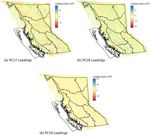
Fig. A1 The spatially reconstructed loadings of the leading four eigenvectors from principal component analysis of the $\mathrm{S}{\mathrm{D}}_{\mathrm{o}\mathrm{f}\mathrm{f}}$ time series, years 2000–2018.

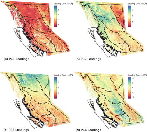
Fig. A2 The spatially reconstructed loadings of the leading four eigenvectors from principal component analysis of the $\mathrm{S}{\mathrm{D}}_{\mathrm{o}\mathrm{f}\mathrm{f}}$ time series, years 2000–2018.

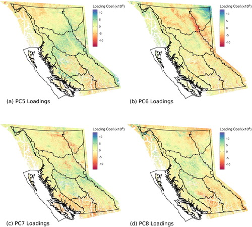
Fig. A3 The spatially reconstructed loadings of the leading four eigenvectors from principal component analysis of the $\mathrm{S}{\mathrm{D}}_{\mathrm{o}\mathrm{f}\mathrm{f}}$ time series, years 2000–2018.

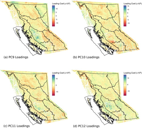
Fig. A4 The spatially reconstructed loadings of the leading four eigenvectors from principal component analysis of the $\mathrm{S}{\mathrm{D}}_{\mathrm{o}\mathrm{f}\mathrm{f}}$ time series, years 2000–2018.

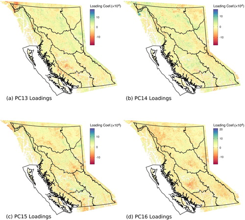
Fig. A5 The spatially reconstructed loadings of the leading four eigenvectors from principal component analysis of the $\mathrm{S}{\mathrm{D}}_{\mathrm{o}\mathrm{f}\mathrm{f}}$ time series, years 2000–2018.

Appendix B: Mean Sea Level Pressure Spatial Loadings

Fig. B1 Spatially reconstructed PC1, PC2, PC3, and PC8, loadings from PCA of the $\mathrm{M}\mathrm{S}\mathrm{L}{\mathrm{P}}_{\mathrm{F}\mathrm{A}\mathrm{L}\mathrm{L}}$ time series (1979–2018). Units are dimensionless.

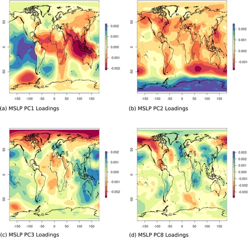
Fig. B2 Spatially reconstructed PC10 and PC11 loadings from PCA of the $\mathrm{M}\mathrm{S}\mathrm{L}{\mathrm{P}}_{\mathrm{F}\mathrm{A}\mathrm{L}\mathrm{L}}$ time series (1979–2018). Units are dimensionless.

References

- Bevington, A. R., Gleason, H. E., Foord, V. N., Floyd, W. C., & Griesbauer, H. P. (2019). Regional influence of ocean-climate teleconnections on the timing and duration of MODIS derived snow cover in British Columbia, Canada. The Cryosphere Discussions, 2019, 1–30. https://doi.org/10.5194/tc-13-2693-2019
- Bozdogan, H. (2003). Intelligent statistical data mining with information complexity and genetic algorithms. In H. Bozdogan (Ed.), Statistical data mining and knowledge discovery (pp. 15–56). Chapman & Hall/CRC.
- Chung, C., & Nigam, S. (1999). Weighting of geophysical data in principal component analysis. Journal of Geophysical Research: Atmospheres, 104(D14), 16925–16928. https://doi.org/10.1029/1999JD900234
- Cohen, J. (1994). Snow cover and climate. Weather, 49(5), 150–156. https://rmets.onlinelibrary.wiley.com/doi/abs/10.1002/j.1477-8696.1994.tb05997.x https://doi.org/10.1002/j.1477-8696.1994.tb05997.x
- Demšar, U., Harris, P., Brunsdon, C., Fotheringham, A. S., & McLoone, S. (2012). Principal component analysis on spatial data: An overview. Annals of the Association of American Geographers, 103(1), 106–128. https://doi.org/10.1080/00045608.2012.689236
- ECMWF. (2020). ERA5. https://www.ecmwf.int/en/forecast/dataset/reanalysis-datasets/eras
- Fisher, R. A. (1936). The use of multiple measurements in taxonomic problems. Annals of Eugenics, 7(2), 179–188. https://doi.org/10.1111/j.1469-1809.1936.tb02137.x
- Gotelli, N. J., & Ellison, A. M. (2013). A primer of ecological statistics (2nd ed). Sinauer Associates, Inc.
- Hall, O. K., & Riggs, G. A. (2016a). MODIS/Terra snow cover daily L3 global 500 m SIN grid, version 6. Retrieved January 1, 2019 from https://nsidc.org/data/modioa1
- Hall, O. K., & Riggs, G. A. (2016b). MODIS/Aqua snow cover daily L3 global 500 m SIN grid, version 6. Retrieved January 1, 2019 from https://nsidc.org/data/modia2
- Hartigan, J. A., & Wong, M. A. (1979). A K-means clustering algorithm. Journal of the Royal Statistical Society: Series C (Applied Statistics), 28(1), 100–108. https://doi.org/10.2307/2346830
- Hersbach, H., Bell, W., Berrisford, P., Horányi, A., Sabater, J. M., Nicolas, J., Radu, R., Schepers, D., Simmons, A., Soci, C., & Dee, D. (2019, 04). Global reanalysis: Goodbye ERa-Interim, hello ERA5. ECMWF newsletter, 17–24. https://www.ecmwf.int/node/19027
- Horel, J. D., & Wallace, J. M. (1981). Planetary-scale atmospheric phenomena associated with the Southern Oscillation. Monthly Weather Review, 109(4), 813–829. https://doi.org/10.1175/1520-0493(1981)109<0813:PSAPAW>2.0.CO;2
- Huang, B., Thorne, P. W., Banzon, V. F., Boyer, T., Chepurin, G., Lawrimore, J. H., Menne, M. J., Smith, T. M., Vose, R. S., & Zhang, H.-M. (2017). Extended reconstructed sea surface temperature, version 5 (ERSSTv5): Upgrades, validations, and intercomparisons. Journal of Climate, 30(20), 8179–8205. https://doi.org/10.1175/JCLI-D-16-0836.1
- John, C., Miller, D., & Post, E. (2020). Regional variation in green-up timing along a caribou migratory corridor: Spatial associations with snowmelt and temperature. Arctic, Antarctic, and Alpine Research, 52(1), 416–423. https://doi.org/10.1080/15230430.2020.1796009
- Kshirsagar, A. M., & Arseven, E. (1975). A note on the equivalency of two discrimination procedures. The American Statistician, 29(1), 38–39. https://doi.org/10.1080/00031305.1975.10479111
- Latif, M., Anderson, D., Barnett, T., Cane, M., Kleeman, R., Leetmaa, A., Brien, J., Rosati, A., & Schneider, E. (1998). A review of the predictability and prediction of ENSO. Journal of Geophysical Research: Oceans, 103(C7), 14375–14393. https://doi.org/10.1029/97JC03413
- Mahalanobis, P. C. (2018). On the generalized distance in statistics. Sonkhya A, 80, 1–7. (Original work published in 1936). https://doi.org/10.1007/s13171-019-00164-5
- Mantua, N., Hare, S., Zhang, Y., Wallace, J., & Francis, R. (1997). A Pacific interdecadal climate oscillation with impacts on salmon production. Bulletin of the American Meteorological Society, 78(6), 1069–1079. https://doi.org/10.1175/1520-0477(1997)078<1069:APICOW>2.0.CO;2
- Ministry of Environment and Climate Change Strategy. (2011). Ecoprovinces - Ecoregion Ecosystem Classification of British Columbia. https://catalogue.data.gov.bc.ca/dataset/ecoprovinces-ecoregion-ecosystem-classification-of-british-columbia
- Mitchell, M. (1998). An introduction to genetic algorithms. A Bradford Book The MIT Press.
- Moore, R., & McKendry, I. (1996). Spring snowpack anomaly patterns and winter climatic variability, British Columbia, Canada. Water Resources Research, 32(3), 623–632. https://doi.org/10.1029/95WR03640
- R Core Team. (2019). R: A language and environment for statistical computing [Computer software manual]. Vienna, Austria. https://www.R-project.org/
- Regonda, S. K., Rajagopalan, B., Clark, M., & Zagona, E. (2006). A multimodel ensemble forecast framework: Application to spring seasonal flows in the Gunnison River Basin. Water Resources Research, 42(9), 1–14. https://doi.org/10.1029/2005WR004653
- Richman, M. (1986). Rotation of principal components. Journal of Climatology, 6(3), 293–335. https://doi.org/10.1002/joc.3370060305
- Riggs, G. A., Hall, D. K., & Román, M. O. (2016). MODIS snow products collection 6 user guide. National Aeronautics and Space Administration. https://modis-snow-ice.gsfc.nasa.gov/uploads
- Rousseeuw, P. J. (1987). Silhouettes: A graphical aid to the interpretation and validation of cluster analysis. Journal of Computational and Applied Mathematics, 20, 53–65. https://doi.org/10.1016/0377-0427(87)90125-7
- Scrucca, L. (2013). GA: A package for genetic algorithms in R. Journal of Statistical Software, 53(4), 1–37. https://doi.org/10.18637/jss.v053.i04
- Shabbar, A. (2006). The impact of El Niño-Southern Oscillation on the Canadian climate, Advances in Geosciences 6, 149–153. https://doi.org/10.5194/adgev-6-149-2006
- Shabbar, A., & Khandekar, M. (1996). The impact of El Niño-Southern Oscillation on the temperature field over Canada: Research note. Atmosphere-Ocean, 34(2), 401–416. https://doi.org/10.1080/07055900.1996.9649570
- Stahl, K., Moore, R., & McKendry, I. (2006, 03). The role of synoptic-scale circulation in the linkage between large-scale ocean-atmosphere indices and winter surface climate in British Columbia, Canada. International Journal of Climatology, 26(4), 541–560. https://doi.org/10.1002/joc.1268
- Thompson, D. W. J., & Wallace, J. M. (2000, 03). Annular modes in the extratropical circulation. Part I: Month-to-month variability. Journal of Climate, 13(5), 1000–1016. https://doi.org/10.1175/1520-0442(2000)013<1000:AMITEC>2.0.CO;2
- Trenberth, K. E. (1976). Spatial and temporal variations of the Southern Oscillation. Quarterly Journal of the Royal Meteorological Society, 102(433), 639–653. https://doi.org/10.1002/qj.49710243310
- Venables, W. N., & Ripley, B. D. (2002). Modern applied statistics with S (4th ed.). Springer.
Appendix A
Spatial Loadings