The Pleistocene Glacial Cycles and Millennial-Scale Climate Variability

ABSTRACT

The Pleistocene glacial cycles are the most prominent climate variations over the past three million years. They are the climatic response to variations in the incoming solar radiation, insolation, due to the deviations of the Earth's orbital configuration from the perfect Keplerian orbit is caused by the influence of the other planets in the solar system. This climatic response to astronomical forcing is highly non-linear, which is most pronounced expressed in the changing duration of the glacial cycles through the Middle Pleistocene Transition around a million years ago, where the duration of glacial cycles changed from 40 kyr to approximately 100 kyr without any corresponding changes in the astronomical forcing. In the late Pleistocene glaciations, the Northern Hemisphere ice sheets have grown larger than before, causing an increased cooling through the ice-albedo feedback, which makes it harder with increased insolation to cause deglaciation. The cold climate with extended glaciations has also made the climate more unstable, where strong millennial-scale oscillations related to changes in the Atlantic Meridional Overturning Circulation are observed in the paleoclimatic records.

RÉSUMÉ

[Traduit par la rédaction] Les cycles glaciaires du Pléistocène constituent les variations climatiques les plus importantes des trois derniers millions d'années. Ils sont la réponse climatique aux variations du rayonnement solaire entrant, l'insolation, attribuables aux déviations de la configuration orbitale de la Terre par rapport à l'orbite képlérienne parfaite causée par l'influence des autres planètes du système solaire. Cette réponse climatique au forçage astronomique est hautement non linéaire, ce qui s'exprime le plus clairement dans le changement de la durée des cycles glaciaires pendant la transition du Pléistocène moyen, il y a environ un million d'années, où la durée des cycles glaciaires est passée de 40 kyrs à environ 100 kyrs sans aucun changement correspondant dans le forçage astronomique. Au cours des glaciations de la fin du Pléistocène, les calottes glaciaires de l'hémisphère nord se sont agrandies, provoquant un refroidissement accru par le biais de la rétroaction de l'albédo de la glace, qui rend plus difficile la déglaciation en cas d'augmentation de l'insolation. Le climat froid et l'extension des glaciations ont aussi rendu le climat plus instable, où de fortes oscillations à l'échelle millénaire liées aux changements de la circulation méridienne de retournement de l'Atlantique sont observées dans les archives paléoclimatiques.

KEYWORDS:

• glacial cycles
• ice age models
• Milankovitch theory
• millennial-scale climate variability
• ice core records
• dynamical climate models

1 Climate of the plio-pleistocene and glacial cycles

The global deep ocean temperature, in combination with the global ice volume, is recorded in the oxygen isotope ratios in the calcium carbonates from sedimented benthic foraminifera. The combination comes from the biological isotope fractionation in the uptake of sea water by the living plankton, which depends on water temperatures, while the concentration of heavy oxygen isotope water depends on how much, preferentially light, water is deposited in the global ice volume. The sedimentation rate in the deep ocean is very low, of the order a centimetre per millennium, thus deep sea sediment cores covering the full Cenozoic era (66 Ma to present) has been obtained. A stacked record, comprised of several deep sea cores is presented by Zachos et al. (2001) with a detailed account of the variations found in the record. The deep ocean has gradually cooled by up to about 10${}^{\circ }$C through the Cenozoic, with several faster cooling periods when first the East Antarctic, later the West Antarctic ice sheet were formed. Around 34 Myr large glaciations marked the greenhouse-icehouse transition (Katz et al., 2008). The icehouse climate is dominated by glacial cycles in the frequency band of the astronomical variations in Earths orbit (eccentricity), in the inclination of the axis of rotation (obliquity) and the direction of the axis of rotation with respect to the ecliptic plane (precession). These variations cause changing insolation and are thus considered as the astronomical forcing of the climate. The astronomical cause of glaciations was proposed by James Croll among others in the mid-nineteenth century. In the first half of the twentieth century, Milutin Milankovitch developed the theory and calculated the insolation based on celestrial mechanics and combined this with modelling of glaciations on the Earth (Milankovitch, 1930). Today we consider Milankovitch theory of glacial cycles as essentially correct. 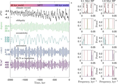Milankovitch calculated the insolation at 65${}^{\circ }$ north latitude at summer solstice (65N ss), arguing together with climatologist Wladimir Köppen that this is the most important place and time for melting of the ice sheets, thus where the climate sensitivity is the highest. The effect of the orbital parameters on the climate response goes via the insolation field, which changes with latitude and season (Berger et al, 2010). It is not obvious which latitude and season would dominate the response. In order to overcome this, Hays et al. (1976) assumed the climate response to be governed by a linear differential equation, in which case the spectral peaks of the response should be related to the spectral peaks of the orbital parameters themselves, though possibly with different gain functions for the different spectral peaks. They found that the climate responds mainly to obliquity and precession. However, when focusing on the last 2 Myr record, it is apparent that there is not a simple linear relationship between the global ice volume and the insolation, neither integrated nor at any specific latitude. Fig. 1 shows the stacked deep sea record compiled by Lisiecki and Raymo (2005) together with the orbital parameters (Laskar et al., 2004) and the 65N ss insolation. The spectral power in the two periods 2-1 My BP (Fig. 1(b)) before the Middle Pleistocene transition (MPT) and 1-0 My BP (Fig. 1(c)) after the MPT are shown. The climate record shows that the 41 kyr obliquity cycle dominates prior to the MPT, while after the transition, glacial ice volumes became larger and glacial periods longer of the order 100 kyr, more in sync with the eccentricity cycle. There is no transition corresponding to the MPT in the astronomical forcing, where the spectra are essentially identical for the two periods (Figs. 1(d,e)). Thus the changing response to the astronomical forcing must be internal to the climate system. We shall discuss the full spectrum later.

Fig. 1 The primary record of the past climate is the ${\delta }^{18}O$ of benthic foraminifera in the deep sea sediments. Top curve in the left panel shows the stacked record of the past 2 Myr (Lisiecki & Raymo, 2005). The record has a dominant cyclicity with a period of 41 kyr prior to the MPT around 1 My BP. After the MPT the glacial cycles became more irregular and lasting approximately 100 kyr. The difference between the two periods is manifested in the power spectra, which show a strong spectral peak at 41 kyr and very little power around 100 kyr prior to the MPT (top right, first panel), while a broad spectral peak occurs around 100 kyr after the MPT, but still with some power in the 41 kyr peak. The orbital parameters and the 65N ss insolation are shown below. For these the spectra before and after the MPT are essentially identical, as seen in the right panels. The vertical red lines indicates periods of 23 kyr (precession), 41 kyr (obliquity) and 100 kyr (eccentricity).

2 The astronomical forcing

Before discussing the modelling of climate response to the astronomical forcing, we shall briefly review the effect of the three orbital parameters, obliquity, eccentricity and precession shown in Fig. 1: Obliquity, with a sharp spectral peak at 41 kyr, determines the magnitude of the seasonal cycle and equator to pole contrast, it is symmetric between the two hemispheres. The eccentricity, with broad spectral peaks around 100 kyr and 400 kyr, determines the envelope of the precessional cycle as is clearly seen in Fig. 1: With a high eccentricity, there is a larger difference between the insolation in summer and winter, depending on if summer is at perihelion (closest to the sun) or at aphelion (farthest from the sun). The effect of eccentricity on seasonal contrast is thus anti-symmetric between the two hemispheres. The precessional cycle, with two spectral peaks close to 19 and 23 kyr, changes the distribution of the insolation through the seasonal cycle and dominates the summer/winter solstice insolation, as can be seen in the similarity between the precession and the 65N ss insolation curves. The rational behind using 65N ss insolation curve as representative of the astronomical forcing is the assumption that the Northern hemisphere ice sheets would be most sensitive to the summer melt at their equator-ward edge. However, as is seen in Fig. 1(b,c), there is very little weight in the precessional band (Fig. 1(h,i)). If instead the annually integrated insolation is considered (not shown), the variations due to precession cancel as a consequence of Keplers second law (Huybers & Wunsch, 2005); The time spend at aphelion is longer than the time spend at perihelion, thus if the summer is weak (aphelion) it is longer and if it is strong (perihelion) it is short. As a consequence, the annually integrated insolation follows the obliquity, which has a substantial weight in the climate spectrum, especially before the MPT (the 40 kyr world). After the MPT the glacial periods became longer, with spectral weight around 100 kyr (the 100 kyr world). With the longer glaciations, the ice sheets became larger, as can be seen in the lower glacial ${\delta }^{18}0$ values in the climate record. Two final remarks on the climate record are the lack of response to the 400 kyr envelope in the eccentricity cycle, sometimes referred to as the Marine Isotope Stage (MIS) 11 problem. This is the interglacial 400 kyr BP at a time when the 65N summer insolation was as low as in other glacial periods. Based on deglaciations over the past 2.6 Myr, Tzedakis et al. (2017) propose a set of conditions for when full deglaciation occurs. The conditions are based on maxima for the caloric summer half-year insolation at 65N, which is dominated by the obliquity cycle. This observation questions the importance of the eccentricity and the precessional cycles as drivers of glacial cycles. Second remark is that the 100 kyr cycles, contrary to the 41 kyr cycles, are very time asymmetric: The glaciations (inceptions) are slow, while the deglaciations (terminations) are fast. There are no correspondences to this time asymmetry in the astronomical forcing.

3 Modelling the glacial cycles

Simulations of the glacial cycles with a comprehensive climate model (Abe-Ouchi et al., 2013) and an intermediate complexity model (Ganopolski et al., 2010) with active ice sheet models have been performed. These are radiatively forced by the insolation and prescribed time-varying greenhouse gas concentrations. Without the latter, the models do not react sufficiently to the orbital forcing. Thus the question of the dominant physical mechanisms in the glacial dynamics is still an open question. Furthermore, rather than pursuing a detailed description of all components of the climate system, better insight into the dynamical mechanisms can be obtained in simpler models with few degrees of freedom. These can be conceptual, such as the stochastic resonance (Benzi et al., 1982), which explains how stochastic noise can amplify a periodic response to a weak periodic forcing. Or they can model a few dominating variables believed to govern the glacial cycles.

Following Imbrie and Imbrie (Imbrie & Imbrie, 1980), the simplest assumption is that the ice volume, y would be linearly responding to the astronomical forcing x, thus in equilibrium with suitable normalization we would have x = y. However, as the forcing is changing there will be a response time τ for the ice sheets to adjust, such that the dynamics would be governed by the linear equation, (1) $\mathrm{d}y/\mathrm{d}t=(x-y)/\tau .$(1) In the case of a sinusoidal forcing $x=\cos \omega t$, the response will be sinusoidal with a lag θ, fulfilling the equation $\tau =\tan \left(\omega \theta \right)/\omega$. Thus from observing the lag between the forcing and the response, the response time τ could be in principle be obtained. It is clear from the climate record showing slow inception and fast termination, that buildup of ice sheets and melting of ice sheets are governed by dynamics with very different time scales. A natural approach to this asymmetry is to assume a piecewise linear model with two time scales ${\tau }_1>{\tau }_2$ for glaciation and deglaciation (Imbrie & Imbrie, 1980): (2) $\begin{array}{rll}\mathrm{d}y/\mathrm{d}t& =(x-y)/{\tau }_1+\eta \left(t\right),x<y& \\ \mathrm{d}y/\mathrm{d}t& =(x-y)/{\tau }_2+\eta \left(t\right),x>y,\end{array}$(2) where the ice sheets are growing when x<y and shrinking when x>y. This leads to an asymmetric response dominated by the transients (solutions to the homogeneous equation) $y=y_0\exp (-t/{\tau }_{1,2})$. Here and in the following $\eta \left(t\right)$ is a white noise with variance ${\sigma }^2$. This can for any model be argued to be a simple representation of the influence of internal climate variability. A conceptual model to explain the late Pleistocene glacial cycles as a response to the orbital forcing was proposed by Huybers and Wunsch (2005). They proposed that the ice volume would be linearly increasing until a time-varying threshold proportional to the obliquity is reached. At that point the ice sheets would collapse linearly over 10 kyr and a new growth cycle would begin.

A dynamical explanation of this kind of dynamical behaviour was already proposed by MacAyeal (1979), who noted that both in the classical global Budyko (1972)- energy balance model and in the Weertman (1976) ice sheet model, fold bifurcations separate two distinct stable states. If the ice-ocean coupling related to isostatic rebound change the dynamics, it was hypothesized that a parameter is slowly changed such that the two states merge through a cusp a periodic change of this slow variable could lead to a smooth glaciation and an abrupt deglaciation. MacAyeal did not propose a dynamics for the slow parameter, but the model is in its simplicity certainly appealing as an explanation for the asymmetry between glaciation and deglaciation.

A slightly more advanced model taking the internal climatic dynamics explicitly into account was proposed by Saltzman (1990); Saltzman and Maasch (1991). In this model, which comes in slightly different versions, three variables; continental ice volume, I, atmospheric CO${}_2$ concentration, μ and deep sea temperature, θ, are described by three coupled ordinary differential equations (Saltzman & Maasch, 1991): (3) $\begin{array}{rll}\mathrm{d}I/\mathrm{d}\tau & =-I-\mu -{\alpha }_1\theta -{\alpha }_{2}F\left(\tau \right)+{\eta }_I\left(t\right)& \\ \mathrm{d}\mu /\mathrm{d}\tau & =-{\text{β}}_1\theta +{\text{β}}_2\mu -{\text{β}}_3{\mu }^2-{\mu }^3+{\eta }_{\mu }\left(t\right)\\ \mathrm{d}\theta /\mathrm{d}\tau & =-{\gamma }_1(I+\theta )+{\eta }_{\theta }\left(t\right),\end{array}$(3) where the variables, $I,\mu ,\theta$ and time, τ are scaled and transformed to a non-dimensional form. 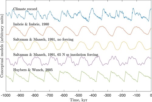$F\left(t\right)$ is the astronomical forcing, while $({\alpha }_1,{\alpha }_2,{\text{β}}_1,{\text{β}}_2,{\text{β}}_3,{\gamma }_1)$ are parameters, where only four are independent. For a heuristic justification of the model see ref. (Saltzman & Maasch, 1991). For relevant parameter values the model exhibits self-sustained oscillations even in the autonomous case of no astronomical forcing. A different internal mechanism for glacial cycles was proposed by Gildor and Tziperman (2000). In a box model of ocean and atmosphere with representation of sea ice and land ice, a feedback loop involving sea ice albedo leading to colder climate and reduced precipitation, leading to reduction of ice sheets and lower ice albedo results in a slow-fast oscillator. Several other oscillator models have been proposed, for a nice overview see ref. (Crucifix, 2012). At the level of reproducing the paleoclimatic record it is difficult to judge the realism in one simple model over the other. The evolution of the model climate variable for a few of the proposed models are shown together with the climate record in Fig. 2.

Fig. 2 The climate record (Lisiecki & Raymo, 2005) for the past 1 My is compared with a few of the proposed models. In each of the models a small intensity, $\sigma =0.02$ stochastic forcing is applied. In the Imbrie and Imbrie, 1980 model the timescales for glaciation and deglaciation are ${\tau }_1=50$ kyr and ${\tau }_2=2$ kyr (Eq. (1(1) $\mathrm{d}y/\mathrm{d}t=(x-y)/\tau .$(1) )). The Saltzman and Maasch, 1991 model (Eq. (3(3) $\begin{array}{rll}\mathrm{d}I/\mathrm{d}\tau & =-I-\mu -{\alpha }_1\theta -{\alpha }_{2}F\left(\tau \right)+{\eta }_I\left(t\right)& \\ \mathrm{d}\mu /\mathrm{d}\tau & =-{\text{β}}_1\theta +{\text{β}}_2\mu -{\text{β}}_3{\mu }^2-{\mu }^3+{\eta }_{\mu }\left(t\right)\\ \mathrm{d}\theta /\mathrm{d}\tau & =-{\gamma }_1(I+\theta )+{\eta }_{\theta }\left(t\right),\end{array}$(3) )) is shown with parameters $({\alpha }_1,{\text{β}}_1,{\text{β}}_2,{\text{β}}_3,{\gamma }_1)=(1.0,2.5,1.3,0.6,0.2)$ and in the two cases ${\alpha }_2=0$ i.e. no astronomical forcing and ${\alpha }_2=0.5$ with the astronomical forcing $F\left(\tau \right)$ being the 65 N ss insolation normalized to zero mean and unit variance. The dimensionless time is $\tau =t/10$ kyr. The Huybers and Wunch, 2005 model has a linear drift, which in the case of no noise would produce a glaciation of 90 kyr and a deglaciation of 10 kyr.

A quantitative assessment of the importance of different proposed dominant physical processes, such as ice albedo feedback (Gildor & Tziperman, 2000; Källen et al., 1979), greenhouse gas forcing (Saltzman & Maasch, 1991), changing thermohaline circulation (Broecker, 2000) or ice sheet dynamics (Imbrie & Imbrie, 1979) will ultimately need comprehensive Earth System Model simulations. These may well show that the glacial dynamics cannot be attributed to a single physical mechanism, but is a result of interplay of several climatic factors.

4 The middle pleistocene transition

The change at the MPT has been proposed to be related to the stability of the ice sheet through the rigolith hypothesis (Clark & Pollard, 1998). The idea is that repeated cycles of glaciations flush out the soft bed, rigolith, beneath the ice sheets, such that at some point the land ice is resting on more solid bedrock permitting higher ice sheets to be stable against sliding. Alternatively a gradual millennium scale decrease in the atmospheric CO${}_2$ concentration would cool the Earth enough for the big post-MPT ice sheets to form Tziperman and Gildor (2003) or it could be a combination of both (Willeit et al., 2019). Atmospheric CO${}_2$ concentrations are reconstructed from Antarctic ice-cores (Lüthi, 2008), but presently only going back 800 kyr, thus not past the MPT. Reconstructions from soil respired CO${}_2$ in paleosols questions a higher atmospheric CO${}_2$ concentration in the early Pleistocene (Da et al., 2019), thus without better reconstruction of the past climate conditions, this is still an open question. However, regardless the cause, the occurrence of the MPT shows that ice age dynamics change as a function of changes at tectonic time scales, independent of the astronomical forcing. The model, Eq. (3(3) $\begin{array}{rll}\mathrm{d}I/\mathrm{d}\tau & =-I-\mu -{\alpha }_1\theta -{\alpha }_{2}F\left(\tau \right)+{\eta }_I\left(t\right)& \\ \mathrm{d}\mu /\mathrm{d}\tau & =-{\text{β}}_1\theta +{\text{β}}_2\mu -{\text{β}}_3{\mu }^2-{\mu }^3+{\eta }_{\mu }\left(t\right)\\ \mathrm{d}\theta /\mathrm{d}\tau & =-{\gamma }_1(I+\theta )+{\eta }_{\theta }\left(t\right),\end{array}$(3) ), undergoes a Hopf-bifurcation in the unforced case (${\alpha }_2=0$), from a fixed point to a limit cycle when changing the parameter ${\text{β}}_1$ through a critical value. Thus Saltzman and Maasch suggested the pre-MPT glacial cycles to be a simple linear response to the obliquity forcing, with a Hopf-bifurcation at the MPT and self-sustained 100 kyr oscillations after the MPT. Still with room for a simple linear response to the obliquity forcing, as long as it do not interfere with the 100 kyr internal oscillation.

As an alternative explanation, Paillard (1998) proposed a conceptual model based on the assumption that the climate is shifting between (quasi-)stable states, a glacial g and an interglacial i, reflecting that the pre-MPT climate is a non-linear response to the obliquity cycle (Ashkenazy & Tziperman, 2004). At the MPT conditions changed, such that larger ice sheets could grow, and a colder glacial state G became accessible. Paillard made the important observation that the pre-MPT climate cycles $i\to g\to i$ changed to $i\to g\to G\to i$ in the post-MPT cycles. It seemed as if there was a rule that the $g\to i$ and $G\to g$ transitions were “forbidden”. With this rule-based model and a threshold for jumping depending on the astronomical forcing, Paillard could reproduce the glacial cycles before and after the MPT. This kind of dynamical behaviour is found in slow-fast dynamical systems where the slow dynamics on a so-called slow manifold is determined by folds and cusps in the manifold. These leads to the specific bifurcation structure, which can explain the “rules” observed (Ditlevsen, 2009). A conceptual dynamical slow-fast internal oscillator on top of the simple model (1(1) $\mathrm{d}y/\mathrm{d}t=(x-y)/\tau .$(1) ) reproduce the Pleistocene climate with the MPT as a transcritical bifurcation without the need for astronomical forcing to reproduce the climate record (Ashwin & Ditlevsen, 2015).

The possibility of an internal oscillator in the climate system itself with a frequency not to far from the astronomical frequencies could explain a climate response to a weak forcing through the phenomenon of frequency locking (Nyman & Ditlevsen, 2019). This could explain the late Pleistocene 100 kyr cycles also as a response to the 41 kyr obliquity forcing. The assumption is that the late Pleistocene glacial cycles are rather 80 kyr and 120 kyr as 2:1 and 3:1 frequency locking of the climate oscillator to the 40 kyr obliquity cycle (Ditlevsen & Ashwin, 2018) in accordance with the suggestion by Huybers and Wunsch (2005). This mechanism is illustrated by the forced Van der Pol oscillator (Crucifix, 2012) in Fig. 3 together with the other proposed mechanisms.

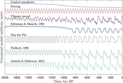
Fig. 3 The MPT is assumed to be caused by a slow, tectonic timescale change in conditions, represented by a “control parameter”, which changes across the MPT (top blue curve). There is no change in the astronomical forcing, here represented by a harmonic 41 kyr oscillation, representing the obliquity. The noisy climate record (Lisiecki & Raymo, 2005) change from 40 kyr to 100 kyr cycles at the MPT. The models are reacting to the changing control parameter and the forcing in dynamically different ways: In the Saltzman & Maasch model (Eq. (3(3) $\begin{array}{rll}\mathrm{d}I/\mathrm{d}\tau & =-I-\mu -{\alpha }_1\theta -{\alpha }_{2}F\left(\tau \right)+{\eta }_I\left(t\right)& \\ \mathrm{d}\mu /\mathrm{d}\tau & =-{\text{β}}_1\theta +{\text{β}}_2\mu -{\text{β}}_3{\mu }^2-{\mu }^3+{\eta }_{\mu }\left(t\right)\\ \mathrm{d}\theta /\mathrm{d}\tau & =-{\gamma }_1(I+\theta )+{\eta }_{\theta }\left(t\right),\end{array}$(3) )) the parameter ${\text{β}}_1$ changes linearly with the control parameter and the model undergoes a Hopf-bifurcation from a fixed point before the MPT to a limit cycle after the MPT. The astronomical forcing results just in a linear response (solutions with and without forcing are shown). In the Van der Pol oscillator the slowly changing parameter controls the period of the oscillator, which is longer than 41 kyr. The oscillator locks to the forcing which, when the internal frequency becomes much longer than the period of the forcing results in a 2:1 and 3:1 frequency locking. In the Paillard model the control parameter determines the threshold ice volume after which the climate will jump into the deep glacial state. In the Ashwin & Ditlevsen model, the system undergoes a transcritical transition at the MPT.

The extent to which the Pleistocene glacial cycles is a response to the astronomical forcing, rather than solely internal oscillation was questioned by Wunsch (2003), who estimated the spectral power in the frequency band corresponding to the astronomical frequencies to be as low as 15% of the total power. This is estimated as the integral of the power in three narrow windows around the astronomical frequencies (red lines in the top left panels in Fig. 1. Fig. 4 is a presentation of the power spectrum in a log-log plot with narrow bands around the astronomical frequencies marked by the grey bars.

Fig. 4 The power spectrum of the climate record where the continuous part of the spectrum is emphasised. The smooth curve is the power spectrum for the red noise or Ornstein-Uhlenbeck process with a correlation time of 100 kyr.

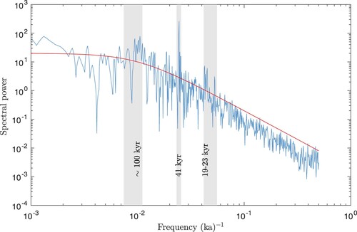
The spectrum is comprised of narrow peaks, which are responses to periodic forcing and a continuous background, reflecting the stochastic nature of the climate. Though dating uncertainty and noise in the proxy-record unrelated to climate tends to broaden a narrow peak spectrum (Ditlevsen et al., 2020), the Pleistocene climate spectrum, blue curve in Fig. 4, is dominated by the continuous background and well captured by the spectrum obtained for the linear stochastic Ohrnstein-Uhlenbeck process (red curve in Fig. 4) as suggested by Hasselmann (1976): (4) $\mathrm{d}x/\mathrm{d}t=-x/\tau +\eta \left(t\right),$(4) where x represents the climate variable, τ is the correlation time and $\eta \left(t\right)$ is a white noise. The correlation time, which signifies the cross-over from a red noise ($P\left(f\right)\sim f^{-2}$) to a white noise $P\left(f\right)\sim const.$) spectrum is around 100 kyr corresponding to the late Pleistocene glacial cycles.

5 Millennial-scale climate variability

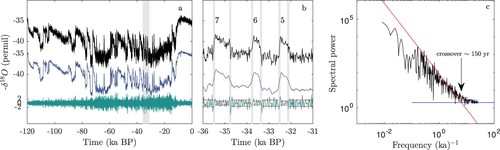
The temporal resolution in the deep sea sediment records is multi-millennial. High sedimentation rate records are found on the continental shelves (Shackleton et al., 2000), but for decadal to millennial-scale variability, the most accurate records are those of Antarctic and Greenland ice cores (Dansgaard et al., 1993; EPICA Community Members, 2004). The main climate variable in ice cores is the depletion of heavy oxygen or deuterium isotope water in comparison with ocean water. In contrast to the sediment records the ice cores can be accurately dated by counting seasonally layered deposits of dust on the ice sheets, which is not diffused in the top firn layer of the ice sheet before being compactified to solid ice. In this way, the North Greenland Icecore Project (NGRIP) (North GRIP Members, 2004) ice-core covering the past 120 kyr has been well dated for the past 60 kyr (Svensson et al., 2008) with an extension of the dating based on ice flow modelling and accumulation rates. Besides the glacial/interglacial cycle itself, the most prominent features of the climate record are the millennial scale Dansgaard-Oeschger (DO) events during the last glacial period. The DO events are abrupt events of 5–10 K warming over less than a decade, followed by gradual cooling lasting from centuries to multi-millennia, called interstadial climate states, until the climate cools rapidly back to the glacial climate, called the stadial states (Lohmann and Ditlevsen, 2019a). In ocean sediment cores covering the past glacial period approximately 10 layers of ice-rafted debris are found. These are the Heinrich events (Heinrich, 1988), where massive amounts of icebergs were released into the North Atlantic. Though synchronizing ocean cores and icecores accurately is an issue, the Heinrich events seem to be connected to the DO events in the sense that the Heinrich events exclusively occur in the stadial states.

Fig. 5(a) shows the GRIP ${\delta }^{18}O$ isotope record covering the last glacial cycle over the past 120 kyr (black curve). The power spectrum in Fig. 5(c) shows a red noise spectrum (red line) consistent with the ocean sediment record, but this high temporal resolution record shows a cross over to a white noise spectrum (blue line) around 150 years. The record in Fig. 5(a) is split into a 150 year running mean (blue curve) and the high pass residual (green curve). The grey band in Fig. 4(a) is blown up in Fig. 5(b), which shows DO events 5–7. The high pass signal (green) represents annual to multi-decadal variability, which is larger in cold (stadial states than in the warm (interstadial) states. The standard deviations are indicated by the red lines in Fig. 5(b).

Fig. 5 Panel a. shows the NGRIP ${\delta }^{18}O$ climate record (North GRIP Members, 2004) at 20 yr resolution covering the past 120 kyr (top curve). The middle curve is the 150 years running mean (low pass), while the green curve is the high pass residual. The DO events are retained in the low pass signal, while the high pass signal contains decadal scale climate fluctuations, which are larger in the cold stadial climate than in the warm interstadial climate. A standard deviation for the two states are indicated by red lines in panel b. with is a blowup of the period indicated by the vertical grey bar in panel a. Panel c. is the power spectrum of the record, consistent with the power spectrum for the ocean sediment record in Fig. 4. For time scales around 150 yr the red noise spectrum, indicated by the red line, crosses over to a white noise spectrum, indicated by the blue line.

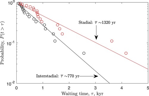
Over the period 60-20 kyr BP, the abrupt shifts between the stadial and the interstadial climate states seems regular to such an extend that it was proposed to be a periodic oscillation (Schulz, 2002). However, as can be seen from Fig. 6, the distribution of waiting times between jumps is consistent with a realization of a stochastic memoryless process (a Poisson process) (Ditlevsen et al., 2007, 2005).

Fig. 6 The waiting time distribution in the period 60-20 kyr BP. Red circles are durations of stadial periods, corresponding to the waiting time before an abrupt jump into the interstadial state. The red line corresponds to an exponential distribution $P(t>\tau )=\exp -\tau /\overline{\tau }$, with mean waiting time $\overline{\tau }=1320$ yr. Black circles and lines are the same for the interstadials, with $\overline{\tau }=770$ yr.

The exponential waiting time distribution indicates a stochastic jump process with an effective dynamics, which can be described as an extension of the red-noise stochastic climate model to the non-linear case, where the drift term corresponds to jumping in a double-well potential.

a Cause of Dansgaard-Oeschger events

Periodically growing and surging ice sheets have been proposed for explaining reoccurring Heinrich events (MacAyeal, 1993). For the DO events several causes have been suggested, but there seems to be a converging consensus that the bi-modal nature of the Atlantic meridional overturning circulation (AMOC) (Manabe & Stouffer, 1988) plays a key role. The fact that DO-events occur exclusively in the glacial climate furthermore indicating that the ice sheets and the extended sea ice cover also play important roles (Li & Born, 2019). The DO-events have been reproduced in in the Community Earth System Model (CESM) (Gent, 2011) applied to glacial conditions (Peltier & Vettoretti, 2014). In the model, the DO-events are caused by a salt oscillator regulating the deep water formation. This oscillator does, furthermore, depend on the atmospheric temperature, which, in turn, depends on the CO${}_2$ concentration. For low concentrations, the climate will reside permanently in the cold stadial state, while for high concentrations, the climate will reside permanently in the warm interstadial state. In an intermediate range of concentrations, the DO oscillator is active (Vettoretti et al., 2022). The oscillator is of the slow-fast system type (Lohmann and Ditlevsen, 2019b). The irregularity in the duration of interstadial and stadial states suggests that internal noise (Berglund & Gentz, 2006) plays an important role in the process as well. Based on the classical Stommel model (Stommel, 1961), the two state dynamics can be described by an effective stochastic equation (Cessi, 1994; Ditlevsen, 1999): (5) $\mathrm{d}x/\mathrm{d}t=-\mathrm{d}U(x,\lambda )/\mathrm{d}x+\eta \left(t\right),$(5) where $U\left(x\right)$ is an effective double-well 'climate potential', typically modelled as $U(x,\lambda )=x^4/4-x^2/2+\lambda x$. This can be seen as a non-linear extension of Eq. (4(4) $\mathrm{d}x/\mathrm{d}t=-x/\tau +\eta \left(t\right),$(4) ). The parameter λ determines the number of stable climate states. For $\left|\lambda \right|>{\lambda }_c(=2/(3\sqrt{3})$ in this case), the system has only one stable climate state, the cold state when $\lambda <-{\lambda }_c$ and the warm state when $\lambda >{\lambda }_c$. For $-{\lambda }_c<\lambda <{\lambda }_c$, both climate states exist. Assuming a time-dependent potential $U(x,\lambda (t\left)\right)=x^4/4-x^2/2+\lambda \left(t\right)x$ and $\lambda \left(t\right)$ passing through ${\lambda }_c$, the system undergoes a fold-bifurcation, where one stable state disappears and the climate jumps to the other climate state. Such a transition is denoted a “b-tipping” (“b” for bifurcation), while if $\left|\lambda \right(t\left)\right|<{\lambda }_c$ as the system jumps from one climate state to the other caused by the noise in Eq. (5(5) $\mathrm{d}x/\mathrm{d}t=-\mathrm{d}U(x,\lambda )/\mathrm{d}x+\eta \left(t\right),$(5) ), this is called an “n-tipping” (“n” for noise). In the real climate system, transitions are probably a combination of the two tipping scenarios. The most striking effect of such a combination is the stochastic resonance phenomenon (Benzi et al., 1982). With a periodic change of the parameter $\lambda \left(t\right)=A\cos \omega t$ and $A<{\lambda }_c$, the system is periodically approaching, but not reaching the bifurcation point, but with a suitable intensity of the noise (thus “resonance”), the system will jump by n-tipping in synchrony with the periodic change of $\lambda \left(t\right)$ (the forcing). The apparent regularity of the DO events has been suggested to be caused by stochastic resonance (Alley et al., 2001). However, since the regularity of the DO events is probably by chance (Ditlevsen et al., 2005), and there are no known external forcing at the millennial time scale, this is an unlikely scenario. The question of identifying the DO-events as either b-tipping or n-tipping is important from the perspective of predictability. In a b-tipping scenario, where the slowly changing control parameter $\lambda \left(t\right)$ approach the bifurcation point, predictability of the tipping depends on the predictability of $\lambda \left(t\right)$, which of course has to be known from the actual physics in the system. In the n-tipping case, predictability is limited to predicting the noise in the system, which is the internal fast fluctuating forcing from the atmosphere-ocean system. The horizon for prediction is governed by the chaotic nature of the flow and thus very limited. The two scenarios are distinguishable in the climate fluctuations preceeding the tipping: In the b-tipping case there are so-called early warning signals (EWS) for the critical transition (Scheffer et al., 2009). These originate from the very general fluctuation-dissipation theorem (Kubo, 1966), which implies that when approaching a fold-bifurcation, the variance of the signal will diverge, since the steady-state looses its stability. Likewise with the loss of stability, the system looses its tendency to counteract large fluctuations, which results in an increase in the autocorrelation. This is the phenomenon of critical slow down. Such EWS are not observed prior to the DO events, thus pointing to these being noise induced (Ditlevsen & Johnsen, 2010). However, all DO events might not be caused by the same triggering mechanism, and there suggestions that some of the events could have been preceeded by EWS (Boers, 2018).

The stochastic Eq. (5(5) $\mathrm{d}x/\mathrm{d}t=-\mathrm{d}U(x,\lambda )/\mathrm{d}x+\eta \left(t\right),$(5) ) can be seen as a singular limit of the fast-slow dynamical system, with $x\left(t\right)$ being the fast and $\lambda \left(t\right)$ being the slow variable: (6) $\begin{array}{rll}\mathrm{d}x/\mathrm{d}t& =f(x,\lambda )+\eta \left(t\right)& \\ \mathrm{d}\lambda /\mathrm{d}t& =ϵg(x,\lambda ),\end{array}$(6) where ϵ is a small parameter, which signifies the ratio of the timescales of variations $ϵ\sim {\tau }_x/{\tau }_{\lambda }$. The singular limit mentioned above is the limit $ϵ\to 0$, where λ becomes a constant parameter. The dynamics of λ can be understood considering the relevant timescale ${\tau }_{\lambda }={\tau }_x/ϵ$ by a simple transformation of the time variable to the slow timescale $\tau =t/ϵ$, such that Eq. (6(6) $\begin{array}{rll}\mathrm{d}x/\mathrm{d}t& =f(x,\lambda )+\eta \left(t\right)& \\ \mathrm{d}\lambda /\mathrm{d}t& =ϵg(x,\lambda ),\end{array}$(6) ) becomes (7) $\begin{array}{rll}\mathrm{d}x/\mathrm{d}\tau & =ϵf(x,\lambda )+\sqrt{ϵ}\eta \left(\tau \right)& \\ \mathrm{d}\lambda /\mathrm{d}\tau & =g(x,\lambda ),\end{array}$(7) where the limit $ϵ\to 0$ defines the so-called slow manifold defined as $\left\{\right(x,\lambda \left)\right|f(x,\lambda )=0\}$ and the slow dynamics is $\mathrm{d}\lambda /\mathrm{d}\tau =g\left(x\right(\lambda ),\lambda )$ with $f\left(x\right(\lambda ),\lambda )=0$. This type of model includes the fast slow oscillators, such as the FitzHugh-Nagumo model (Lohmann and Ditlevsen, 2019), with $f(x,\lambda )=a_{1}x-a_3{x}^3+a_0+b\lambda$ and $g(x,\lambda )=c_1\lambda -x+c_0$ and $a_0,a_1,a_3,b,c_0,c_1$ being constant parameters. The behaviour of the model can be understood from a phase-space portrait of the two so-called “null-clines”, which are the curves $\left\{\right(x,\lambda \left)\right|f(x,\lambda )=0\}$ and $\left\{\right(x,\lambda \left)\right|g(x,\lambda )=0\}$, where the first is the slow manifold. Fig. 7 shows five sets of models with $g(x,\lambda )=\lambda -x+c_0$ and different values of the parameter $c_0$. In each panel to the right, the grey curve is the slow manifold, while the red line is the other null-cline. The full grey curves are the two stable branches of the slow manifold while the dashed branch is the unstable part. Crossing point(s) of the the two null-clines are fixed points. Only when the crossing is on one of the stable branches, the fix point is stable. When the crossing is on the unstable branch the fixed point is unstable and the solution will be a limit cycle with jumps between the two stable branches. The system resides longer on the stable branch closest to the unstable fixed point. In the left-hand panels realizations of the model with a moderate noise are shown, from bottom to top showing longer and longer interstadials as the parameter $c_0$ changes. This behaviour is found in CESM simulations run under glacial conditions with an inactive ice sheet, where the atmospheric CO${}_2$ concentration is the control parameter, such that for low concentrations, the climate resides in the cold stadial state, while for high concentrations, the climate resides in the warm interstadial climate state. 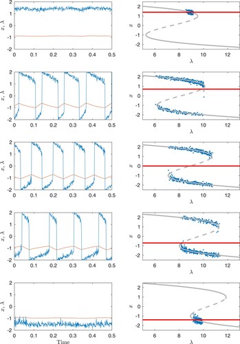In an intermediate window of CO${}_2$ concentrations, the model reproduces DO oscillations (Vettoretti et al., 2022).

Fig. 7 Five realizations of the noisy FitzHugh-Nagumo model with different parameter values for $c_0$ (see text) and null-clines for $\mathrm{d}\lambda /\mathrm{d}t=0\Rightarrow x=c_0$. From bottom and up, $c_0$ is increasing from a situation where the cold climate state is stable, through an oscillator DO phase, to a situation where the warm climate state is stable. The grey curves where $\mathrm{d}x/\mathrm{d}t=0$ are the slow manifold. The blue curves in the left panels are $x\left(t\right)$, while the red curves are the slowly varying $\lambda \left(t\right)$. The blue dots in the right panels are scatter plots of $\left(x\right(t),\lambda (t\left)\right)$.

6 Summary

The most prominent climate variations on multi-millennial time scales over the Pleistocene period are the glacial cycles, where we have looked at the main climate proxy for global ice volume and deep sea temperature, the stacked deep ocean sediment record. There are many other paleoclimatic proxies, which provide more regional climate information, but our focus has been on presenting a very basic understanding of the mechanisms governing the glacial cycles. The strong connection to the astronomical variations in the insolation has been identified already in the nineteenth century, but only now with much more detailed paleoclimatic records, we understand that the connection is far from trivial. Direct simulations with Earth System Models on these long timescales will not be feasible in a foreseeable future, and it is not clear if such a future simulation, reproducing the Pleistocene climate would actually provide the understanding we are seeking. Thus a strategy is to identify robust dynamical mechanisms in conceptual models and to connect these to the dominant governing physical components of the climate system through the hierarchy of models of increasing complexity. Several mechanisms have been proposed and presented here for explaining the MPT, some of which also address the problem of the 100 kyr World. At the millennial timescale, the most prominent climate fluctuations are the Dansgaard-Oeschger and Heinrich events, which are related to the bi-modal nature of the Atlantic Meridional Overturning Circulation coupled to ice sheet and sea ice dynamics. Also here we have focused on presenting possible simple robust dynamical mechanisms. Millennial-scale variability in the Holocene and in parts of the world far away from the “ epi-centre” of DO-events are also important, but unjust ignored here. The proxy records of climate variability on centennial and longer time scales shows a large stochastic component, which is reflected in a large spectral power in the continuous red noise part of the spectrum compared to discrete spectral lines at the astronomical frequencies. However, we also see very abrupt extreme events, such as the DO jumps between the cold and the warm climate states. These can be considered thousand-year events in the sense that the mean waiting time between these events is on the millennial timescale.

Disclosure statement

No potential conflict of interest was reported by the author(s).

Additional information

Funding

This is TiPES contribution no. 160. The TiPES (Tipping Points in the Earth System) project has received funding from the European Union's Horizon 2020 research and innovation program under grant agreement no. 820970.

References

- Abe-Ouchi, A., Saito, F., Kawamura, K., Raymo, M. E., Okuno, J., Takahashi, K., & Blatter, H. (2013). Insolation-driven 100,000-year glacial cycles and hysteresis of ice-sheet volume. Nature, 500(7461), 190–193. https://doi.org/10.1038/nature12374.
- Alley, R. B., Anandakrishnan, S., & Jung, P. (2001). Stochastic resonance in the North Atlantic. Paleoceanography, 16(2), 190–198. https://doi.org/10.1029/2000PA000518.
- Ashkenazy, Y., & Tziperman, E. (2004). Are the 41 kyr oscillations a linear response to Milankovitch forcing? Quaternary Science Reviews, 23(18-19), 1879–1890. https://doi.org/10.1016/j.quascirev.2004.04.008.
- Ashwin, P., & Ditlevsen, P. (2015). The middle Pleistocene transition as a generic bifurcation on a slow manifold. Climate Dynamics, 45, 2683. https://doi.org/10.1007/s00382-015-2501-9.
- Benzi, R., Parisi, G., Sutera, A., & Vulpiani, A. (1982). Stochastic resonance in climate change. Tellus, 34(1), 10–16. https://doi.org/10.1111/j.2153-3490.1982.tb01787.x.
- Berger, A., Loutre, M.-F., & Yin, Q. (2010). Total irradiation during any time interval of the year using elliptic integrals. Quaternary Science Reviews, 29(17-18), 1968–1982. https://doi.org/10.1016/j.quascirev.2010.05.007.
- Berglund, N., & Gentz, B. (2006). Noise-induced phenomena in slow-fast dynamical systems: a sample-paths approach. Springer. https://doi.org/10.1007/1-84628-186-5.
- Boers, N. (2018). Early-warning signals for Dansgaard-Oeschger events in a high-resolution ice core record. Nature Communications, 9, 2556. https://doi.org/10.1038/s41467-018-04881-7.
- Broecker, W. S. (2000). Was changes in the thermohaline circulation responsible for the little ice age?. PNAS, 97(4), 1339–1342. https://doi.org/10.1073/pnas.97.4.1339.
- Cessi, P. (1994). A simple box model of stochastically forced thermohaline flow. Journal of Physical Oceanography, 24(9), 1911–1920. https://doi.org/10.1175/1520-0485(1994)024¡1911:ASBMOS¿2.0.CO;2.
- Clark, P. U., & Pollard, D. (1998). Origin of the middle Pleistocene transition by ice sheet erosion of regolith. Paleoceanography, 13(1), 1–9. https://doi.org/10.1029/97PA02660.
- Crucifix, M. (2012). Oscillators and relaxation phenomena in Pleistocene climate theory. Philosophical Transactions of the Royal Society of London A: Mathematical, Physical and Engineering Sciences, 37(1962), 1140–1165. https://doi.org/10.1098/rsta.2011.0315.
- Da, J., Zhang, Y., Li, G., Meng, X., & Ji, J. (2019). Low CO2 levels of the entire Pleistocene epoch. Nature Communications, 10, 4342. https://doi.org/10.1038/s41467-019-12357-5.
- Dansgaard, W., Johnsen, S. J., Clausen, H. B., Dahl-Jensen, D., Gundestrup, N. S., Hammer, C. U., Hvidberg, C. S., Steffensen, J. P., Sveinbjornsdottir, A. E., Jouzel, J., & Bond, G. (1993). Evidence for general instability of past climate from a 250-kyr ice-core record. Nature, 364, 218–220. https://doi.org/10.1038/364218a0.
- Ditlevsen, P., Mitsui, T., & Crucifix, M. (2020). Crossover and peaks in the Pleistocene climate spectrum; understanding from simple ice age models. Climate Dynamics, 54, 1801–1818. https://doi.org/10.1007/s00382-019-05087-3.
- Ditlevsen, P. D. (1999). Observation of alpha-stable noise and a bistable climate potential in an ice-core record. Geophysical Research Letters, 26(10), 1441–1444. https://doi.org/10.1029/1999GL900252.
- Ditlevsen, P. D. (2009). The bifurcation structure and noise assisted transitions in the Pleistocene glacial cycles. Paleoceanography, 24, PA3204. https://doi.org/10.1029/2008PA001673.
- Ditlevsen, P. D., Andersen, K. K., & Svensson, A. (2007). The DO-climate events are probably noise induced: statistical investigation of the claimed 1470 years cycle. Climate of the Past, 3(1), 129–134. https://doi.org/10.5194/cp-3-129-2007.
- Ditlevsen, P. D., & Ashwin, P. (2018). Complex climate response to astronomical forcing: The Middle-Pleistocene transition in glacial cycles and changes in frequency locking. Frontiers of Physics June. https://doi.org/10.3389/fphy.2018.00062.
- Ditlevsen, P. D., & Johnsen, S. (2010). Tipping points: Early warning and wishful thinking. Geophysical Research Letters, 37(19), L19703. https://doi.org/10.1029/2010GL044486.
- Ditlevsen, P. D., Kristensen, M. S., & Andersen, K. K. (2005). The recurrence time of Dansgaard-Oeschger events and limits on the possible periodic component. Journal of Climate, 18(14), 2594–2603. https://doi.org/10.1175/JCLI3437.1.
- EPICA Community Members (2004). Eight glacial cycles from an Antarctic ice core. Nature, 429, 623–628. https://doi.org/10.1038/nature02599.
- Ganopolski, A., Calov, R., & Claussen, M. (2010). Simulation of the last glacial cycle with a coupled climate ice-sheet model of intermediate complexity. Climate of the Past, 6(2), 229–244. https://doi.org/10.5194/cp-6-229-2010.
- Gent, P. R. (2011). The community climate system model version 4. Journal of Climate, 24(19), 4973–4991. https://doi.org/10.1175/2011JCLI4083.1.
- Gildor, H., & Tziperman, E. (2000). Sea ice as the glacial cycles' climate switch: Role of seasonal and orbital forcing. Paleoceanography, 15(6), 605–615. https://doi.org/10.1029/1999PA000461.
- Hasselmann, K. (1976). Stochastic climate models Part I. Theory. Tellus, 28(6), 473–485. https://doi.org/10.1111/j.2153-3490.1976.tb00696.x.
- Hays, J., Imbrie, J., & Shackleton, N. (1976). Variations in Earth's orbit: Pacemaker of the ice ages. Science, 194(4270), 1121–1132. https://doi.org/10.1126/science.194.4270.1121.
- Heinrich, H. (1988). Origin and consequences of cyclic ice rafting in the Northeast Atlantic Ocean during the past 130000 years. Quaternary Research, 29(2), 143–152. https://doi.org/10.1016/0033-5894(88)90057-9.
- Huybers, P., & Wunsch, C. (2005). Obliquity pacing of the late Pleistocene glacial terminations. Nature, 434, 491–494. https://doi.org/10.1038/nature03401.
- Imbrie, J., & Imbrie, K. P. (1979). Ice ages, solving the mystery. MacMillan Press. ISBN 9780674440753.
- Imbrie, J., & Imbrie, J. Z. (1980). Modeling the climate response to orbital variations. Science, 207(4434), 943–953. https://doi.org/10.1126/science.207.4434.943.
- Källen, E., Crafoord, C., & Ghil, M. (1979). Free oscillations in a climate model with ice-sheet dynamics. Journal of the Atmospheric Sciences, 36(12), 2292–2303. https://doi.org/10.1175/1520-0469(1979)036¡2292:FOIACM¿2.0.CO;2.
- Katz, M., Miller, K., & Wright, J. E. A. (2008). Stepwise transition from the Eocene greenhouse to the Oligocene icehouse. Nature Geoscience, 1, 329–334. https://doi.org/10.1038/ngeo179.
- Kubo, R. (1966). The fluctuation-dissipation theorem. Reports on Progress in Physics, 29, 255–284. https://doi.org/10.1088/0034-4885/29/1/306.
- Laskar, J., Robutel, P., Joutel, F., Boudin, F., Gastineau, M., Correia, A. C. M., & Levrard, B. (2004). A long-term numerical solution for the insolation quantities of the earth. Astronomy and Astrophysics, 428, 261–285. https://doi.org/10.1051/0004-6361:20041335.
- Li, C., & Born, A. (2019). Coupled atmosphere-ice-ocean dynamics in Dansgaard-Oeschger events. Quaternary Science Reviews, 203 (January), 1–20. https://doi.org/10.1016/j.quascirev.2018.10.031.
- Lisiecki, L. E., & Raymo, M. E. (2005). A Pliocene-Pleistocene stack of 57 globally distributed benthic d18O records. Paleoceanography, 20(1), PA1003. https://doi.org/10.1029/2004PA001071.
- Lohmann, J., & Ditlevsen, P. (2019a). Objective extraction and analysis of statistical features of Dansgaard-Oeschger events. Climate of the Past, 15, 1771–1792. https://doi.org/10.5194/cp-15-1771-2019.
- Lohmann, J., & Ditlevsen, P. (2019b). A consistent statistical model selection for abrupt glacial climate changes. Climate Dynamics, 52, 6411–6426. https://doi.org/10.1007/s00382-018-4519-2.
- Lüthi, D. E. A. (2008). High-resolution carbon dioxide concentration record 650,000–800,000 years before present. Nature, 453, 379. https://doi.org/10.1038/nature06949.
- MacAyeal, D. (1979). A catastrophe model of the paleoclimate. Journal of Glaciology, 24(90), 245–257. https://doi.org/10.3189/S0022143000014775.
- MacAyeal, D. R. (1993). Binge/purge oscillations of the Laurentide ice sheet as a cause of the North Atlantic's Heinrich events. Paleoceanography, 8(6), 775–783. https://doi.org/10.1029/93PA02200.
- Manabe, S., & Stouffer, R. J. (1988). Two stable equilibria of a coupled ocean-atmosphere model. Journal of Climate, 1(9), 841–866. https://doi.org/10.1175/1520-0442(1988)001¡0841:TSEOAC¿2.0.CO;2.
- Milankovitch, M. (1930). Mathematiche Klimalehre und Astronomiche Theorie der Klimaschwankungen, Handbuch der Klimalogie Band 1 Teil A, Borntrager Berlin. https://d-nb.info/811073149/04.
- Milankovitch, M. (1941). Kanon der Erdbestrahlung und seine Anwendung auf des Eiszeitenproblem. Special Publication 132, Section of Mathematical and Natural Sciences, Vol. 33, p. 633, 1941. Belgrade: Royal Serbian Academy of Sciences (‘Canon of Insolation and the Ice Age Problem’) (trans. Israel 385 Program for the US Department of Commerce and the National Science Foundation, Washington DC, 1969, and by Zavod za udzbenike i nastavna sredstva in cooperation with Muzej nauke i tehnike Srpske akademije nauka i umetnosti, Beograd, 1998). http://hdl.handle.net/123456789/702.
- Mitsui, T., & Crucifix, M. (2017). Influence of external forcings on abrupt millennial-scale climate changes: A statistical modelling study. Climate Dynamics, 48, 2729–2749. https://doi.org/10.1007/s00382-016-3235-z.
- North GRIP Members (2004). High resolution climate record of the Northern hemisphere reaching into the last glacial interglacial period. Nature, 431, 147–151. https://doi.org/10.1038/nature02805.
- Nyman, K., & Ditlevsen, P. (2019). The middle Pleistocene transition by frequency locking and slow ramping of internal period. Climate Dynamics, 53, 3023–3038. https://doi.org/10.1007/s00382-019-04679-3.
- Paillard, D. (1998). The timing of Pleistocene glaciations from a simple multiple-state climate model. Nature, 391, 378–381. https://doi.org/10.1038/34891.
- Peltier, W. R., & Vettoretti, G. (2014). Dansgaard-Oeschger oscillations predicted in a comprehensive model of glacial climate: A ‘kicked’ salt oscillator in the Atlantic. Geophysical Research Letters, 41(20), 7306–7313. https://doi.org/10.1002/2014GL061413.
- Saltzman, B. (1990). Three basic problems of paleoclimatic modeling: A personal perspective and review. Climate Dynamics, 5, 67–78. https://doi.org/10.1007/BF00207422.
- Saltzman, B., & Maasch, K. A. (1991). A first-order global model of late Cenozoic climatic change. Climate Dynamics, 5, 201–210. https://doi.org/10.1007/BF00210005.
- Scheffer, M., Bascompte, J., Brock, W. A., Brovkin, V., Carpenter, S. R., Dakos, V., Held, H., van Nes, E. H., Rietkerk, M., & Sugihara, G. (2009). Early-warning signals for critical transitions. Nature, 461, 53–59. https://doi.org/10.1038/nature08227.
- Schulz, M. (2002). On the 1470-year pacing of Dansgaard-Oeschger warm events. Paleoceanography, 17(2), 571. https://doi.org/10.1029/2000PA000571.
- Shackleton, N. J., Hall, M. A., & Vincent, E. (2000). Phase relationships between millennial-scale events 64000 to 24000 years ago. Paleoceanography, 15(6), 565–56. https://doi.org/10.1029/2000PA000513.
- Stommel, H. (1961). Thermohaline convection with two stable regimes of flow. Tellus, 13(2), 224–230. https://doi.org/10.1111/j.2153-3490.1961.tb00079.x.
- Svensson, A., Andersen, K. K., Bigler, M., Clausen, H. B., Dahl-Jensen, D., S. M. Davies, Johnsen, S. J., Muscheler, R., Parrenin, F., Rasmussen, S. O., Röthlisberger, R., Seierstad, I., Steffensen, J. P., & Vinther, B. M. (2008). A 60000 year Greenland stratigraphic ice core chronology. Climate of the Past, 4(1), 1–11. https://doi.org/10.1111/j.2153-3490.1961.tb00079.x Citations: 176.
- Tzedakis, P. C., Crucifix, M., Mitsui, T., & Wolff, E. W. (2017). A simple rule to determine which insolation cycles lead to interglacials. Nature, 542, 427–432. https://doi.org/10.1038/nature21364.
- Tziperman, E., & Gildor, H. (2003). On the mid-Pleistocene transition to 100-kyr glacial cycles and the asymmetry between glaciation and deglaciation times. Paleoceanography, 18(1), 1–8. https://doi.org/10.1029/2001pa000627.
- Vettoretti, G., Ditlevsen, P., Jochum, M., & Rasmussen, S. O. (2022). Atmospheric CO2 control of spontaneous millennial-scale ice age climate oscillations. Nature Communications, 15, 300–306. https://doi.org/10.1038/s41561-022-00920-7.
- Weertman, J. (1976). Milankovich solar radiation variations and ice age ice sheet sizes. Nature, 261(5555), 17–20. https://doi.org/10.1038/261017a0.
- Willeit, M., Ganopolski, A., Calov, R., & Brovkin, V. (2019). Mid-Pleistocene transition in glacial cycles explained by declining CO2 and regolith removal. Science Advances, 5(4), 22. https://doi.org/10.1126/sciadv.aav7337.
- Wunsch, C. (2003). The spectral description of climate change including the 100 ky energy. Climate Dynamics, 20(4), 353–363. https://doi.org/10.1007/s00382-002-0279-z.
- Zachos, J., Pagani, M., Sloan, L., Thomas, E., & Billups, K. (2001). Trends, rhythms, and aberrations in global climate 65 ma to present. Science, 292(5517), 686–693. https://doi.org/10.1126/science.1059412.