Full article: Atmospheric Observations of Weather and Climate

Formulae display: $MathJax Logo$ ?Mathematical formulae have been encoded as MathML and are displayed in this HTML version using MathJax in order to improve their display. Uncheck the box to turn MathJax off. This feature requires Javascript. Click on a formula to zoom.

ABSTRACT

Current observation systems that provide data for the analysis and prediction of climate and day-to-day weather are described, along with plans for future systems. The basic principles of satellite, radar, lidar, and sodar measurements are summarized. Temperature and moisture measurements on planetary and synoptic scales, ranging from satellites, the radiosonde network, aircraft, and other sounding systems are described. Wind measurements from satellites, rawinsondes, air composition from satellites, the energy budget, and surface measurements are also discussed. The measuring systems for mesoscale and convective-scale weather are then noted, including satellite-borne radiation instrumentation, and lightning imaging sensors. Operational, fixed-site, and mobile and airborne research radars, surface instrumentation, and ground-based and in-situ profiling systems, aircraft-borne and shipborne instrumentation are also summarized. Special observation issues such as coordination among providers, data assimilation considerations, and data curation are then considered. Special issues for the future are noted in the last section.

RÉSUMÉ

[Traduit par la redaction] Les systèmes d’observation actuels qui fournissent des données pour l’analyse et la prévision du climat et du temps au jour le jour sont décrits, tout comme les plans pour les systèmes ultérieurs. Les principes de base des mesures par satellite, radar, lidar et sodar sont résumés. Les mesures de température et d’humidité à l’échelle planétaire et synoptique, réalisées par les satellites, le réseau de radiosondes, les avions et d’autres systèmes de sondage, sont décrites. Les mesures du vent à partir de satellites, de sondes de radiovent, la composition de l’air à partir de satellites, le bilan énergétique et les mesures de surface sont également abordés. Les systèmes de mesure du temps à méso-échelle et à l’échelle de la convection sont ensuite présentés, y compris les instruments de mesure du rayonnement par satellite et les capteurs d’imagerie de la foudre. Les radars de recherche opérationnels, fixes, mobiles et aéroportés, les instruments de surface, les systèmes de profilage au sol et in situ, les instruments embarqués dans les avions et les navires sont aussi résumés. Les questions d’observation spéciales telles que la coordination entre les fournisseurs, les considérations relatives à l’assimilation des données et la conservation des données sont ensuite examinées. Les questions spéciales pour l’avenir sont indiquées dans la dernière section.

KEYWORDS:

I often say that when you can measure what you are speaking about, and express it in numbers, you know something about it; but when you can not express it in numbers, your knowledge is of a meagre and unsatisfactory kind; … Lord Kelvin, 1883, Physics Letters A, Vol. 1.

1 Introduction

Lord Kelvin would certainly agree that it is vital to measure the state of the atmosphere and its surface boundary in order to understand weather and climate. Physical quantities such as temperature, water vapour, wind speed and direction, pressure, precipitation, cloudiness, radiation, aerosols, atmospheric composition, land and ocean surface properties and many others need to be observed to achieve this understanding. In this review paper, we summarize what is measured and how these measurements are made, thus describing current observational capabilities to define climate, its variability, and its weather extremes.

While the early motivation for meteorological observations was to describe and understand the atmosphere, weather prediction and climate projections are now driving forces for sustaining and increasing our observational capabilities. Prediction of local weather such as severe thunderstorms requires both observations and model grids at sub-kilometer resolution, while climate models benefit from detailed knowledge of atmospheric radiation, aerosols and surface properties. An additional benefit of atmospheric and related observations could be described as situational awareness. Real-time knowledge of potential adverse effects of severe storms, lightning, flooding, fog, smoke, storm surge, etc. are beneficial to forecasters, broadcasters, emergency managers and first responders, utilities, transportation sector, outdoor venues and the general public. Knowledge of weather conditions is important for efficient production of renewable energy, while the changing climate affects energy security. Public health is sensitive to current temperature, humidity, chemistry and aerosol conditions, as well as to a changing climate. Food production and water resource management are also strongly affected by weather and climate variability.

Organizing a review paper on observations is challenging, as it could be done by variable, instrument, purpose, atmospheric location, scientific challenge or operational application. We have chosen a hybrid approach. First, an overview of the basic physical principles governing the primary remote sensing systems is presented. There are separate sections focusing on global observations for climate and synoptic-scale phenomena and their spatiotemporal variability, and on regional observations for mesoscale and convective-scale weather systems. Within these sections, we sequence though the quantities required and the observing systems that provide those measurements. The last major section covers observation-related issues such as coordination, data assimilation, curation and a look forward. We note that since the nature of observing systems is constantly changing and the specific systems operated by different countries and the availability of data vary, this paper will be as generic as possible. However, U. S. systems will often be used as examples. An extensive reference list is provided for those who wish to learn more about each observing system. The reader is also encouraged to search online for information on how to access data from the different observing systems in each country.

2 Observation system fundamentals

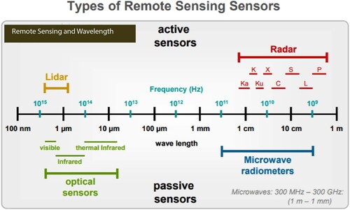
In Section 2 the fundamentals of remote sensors are discussed. The reader is referred to for the frequency ranges of electromagnetic radiation used in many of the sensors; the shortest, visible wavelengths are employed by optical sensors and lidars, while the longest, microwave wavelengths are used by radiometers and radars.

Fig. 1 Types of remote sensing sensors and their wavelengths. (Adapted from , https://earth.esa.int/documents/10174/642943/6-LTC2013-SAR-Moreira.pdf).

Fig. 1 Types of remote sensing sensors and their wavelengths. (Adapted from Fig. 6, https://earth.esa.int/documents/10174/642943/6-LTC2013-SAR-Moreira.pdf).

a Satellites Orbits and Instrumentation Principles

1 Historical note on meteorological satellites

The field of satellite meteorology recently marked the 60th anniversary of the April 1, 1960 launch of the first satellite dedicated to satellite meteorology, the Television and Infrared Observational Satellite (TIROS-1). This event was celebrated in conjunction with the American Geophysical Union (AGU) and American Meteorological Society (AMS) Centennial meetings. Satellite meteorology traces its roots back to the launch of Sputnik on October 4, 1957, soon followed by Explorer 1 launched on January 31, 1958. The history of satellite meteorology with key milestones and instrument advancements is well documented in Smith et al. (Citation1986), Kidder and Vonder Haar (Citation1995), Lewis et al. (Citation2016), Goodman et al. (Citation2018), Menzel (Citation2019), Ackerman et al. (Citation2019), and Vonder Haar et al. (Citation2020). The AMS Monograph by Lewis et al. (Citation2016) is particularly noteworthy as it chronicles the life and times of Professor Verner Suomi, the acknowledged father of satellite meteorology and the co-inventor of the first cloud camera in geosynchronous earth orbit. The camera was carried on the Advanced Technology Satellite (ATS-1) launched in1966 as a research pathfinder. The routine sequence of cloud images possible from high above Earth provided the first depictions of synoptic scale motions from space. GOES-1, the first NOAA Geostationary Operational Environmental Satellite launched on October 16, 1975, initiated a series of operational satellites in geostationary orbit that followed to this day. Of additional historical note are the anthology sessions recorded at the 2019 Joint AMS-EUMETSAT-NOAA Satellite Conference (Session 10) held October 2, 2019 “Celebrating the 60th Anniversary of the First Weather Satellite, its Evolution, and International Partnership” (https://ams.confex.com/ams/JOINTSATMET/meetingapp.cgi/Session/52323) and the 16th Annual Symposium on New Generation Operational Environmental Satellite Systems (Session 3) held with the AMS Annual Meeting on January 13, 2020 (https://ams.confex.com/ams/2020Annual/meetingapp.cgi/Session/53293). These presentations cover the evolution and improvement of the satellite capabilities, instruments, and measurements since the inception of satellite meteorology.

2 Satellite orbits

Weather satellites are the omnipresent backbone of the global observing system (). The principal satellite orbits are Low Earth Orbit (LEO) and Geostationary Earth Orbit (GEO), which together provide different perspectives of the atmosphere and earth below (World Meteorological Organization Space Programme, Citation2020).

Fig. 2 Space-based component of the global observing system (source, WMO Space Program).

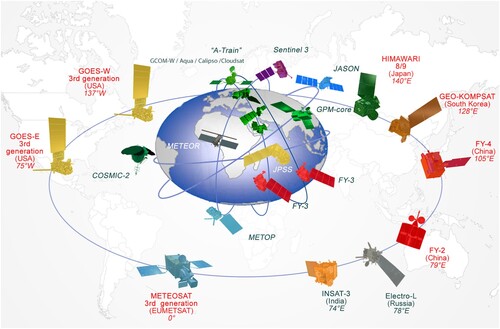
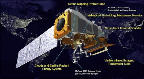
The satellite constellations are used synergistically, from short-term diagnostics of high impact environmental weather such as tropical storms and hurricanes, severe local storms, lightning, advection and radiation fog, aerosols, fire smoke and dust to global numerical weather prediction (NWP) and climate monitoring (see ). The primary source of synoptic-scale global satellite observations of temperature and moisture for NWP are provided by the polar-orbiting operational environmental satellite (POES) constellation infrared and passive microwave sounders in LEO (Goldberg et al., Citation2018; Schumann Citation2020), whereas the GEO satellites are the primary source of near real-time imagery used for nowcasting and the detection of rapidly evolving high impact environmental phenomena (Goodman et al., Citation2018, Citation2019; Holmlund et al., Citation2021; Schmit et al., Citation2017, Citation2018). The major U.S. operational contributions to the baseline satellite observing system depicted in are the Geostationary Operational Environmental Satellite (GOES) – R Series in GEO () and Joint Polar Satellite System (JPSS) in LEO (). A “constellation” of satellites can also fly in formation to produce synchronized data from a collection of different instruments (e.g. the “A/C-train” constellation in comprised of OCO-2, G-COMW, Aqua, Calipso, Cloudsat; https://atrain.nasa.gov, Stephens et al., Citation2018).

Fig. 3 The Geostationary Operational Environmental Satellite (GOES) R-Series satellite and instruments. Graphic courtesy of Lockheed Martin and the GOES-R Program.

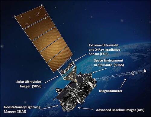
Fig. 4 The Joint Polar Satellite System (JPSS) satellite and instruments. Graphic courtesy of Joseph Smith and the JPSS Program.

The GEO and LEO earth viewing instruments are described below, with further information on the missions, satellites, instruments, data products, and additional resources available at http://goes-r.gov and https://jpss.noaa.gov.

The sun-synchronous LEO orbit has 14 polar-orbiting passes per day with equatorial crossing times at the same time in the morning and afternoon. These orbits provide global imagery, atmospheric data (temperature, moisture, trace gases), and surface (sea and lake ice, ocean salinity and heat content, harmful algae blooms, vegetation health, flood inundation) observations from an altitude of ∼800 km. These measurements are also assimilated into the regional and global NWP models (e.g. European Meteorological Operational satellite (METOP), NOAA’s JPSS, CMA/NSMC (China Meteorological Administration/National Satellite Meteorological Center) Fēngyún-3 (FY-3) in ). LEO orbits can also be precessing where the ground track varies day to day allowing observations throughout the diurnal cycle rather than the twice per day sun-synchronous coverage in polar orbits. The non-sun-synchronous, inclined orbits in LEO have more frequent lower latitude coverage typically from an orbital altitude of about 400 km, but with a longer revisit time to view the same exact spot on the Earth.

GEO satellites are located at 35,786 km (22,236 miles) above the earth’s equator with the orbit matching the Earth's rotation. This allows the satellite to view the earth, atmosphere, and high impact weather at the same satellite sub-point continuously day and night. Together the LEO and GEO orbits and their instruments provide a broad spectrum of atmospheric, land, ocean, and ice measurements used in weather forecasting and analysis ( and ). The new generation international “GEO-Ring” satellite constellation provides full disk earth and atmosphere imagery and derived products (e.g. cloud mask, cloud height, cloud phase, precipitable water, stability indices, winds) over the full earth disk every ten minutes and at a high refresh cadence of 1–2.5 min over limited areas.

Table 1. Satellite backbone with specified orbital configuration and measurement approaches (Subcomponent 1), Source WMO WIGOS.

Download CSV Display Table

Table 2. Backbone satellite system with open orbit configuration and flexibility to optimize the implementation (Subcomponent 2, Source WMO WIGOS).

Download CSV Display Table

Current and planned constellations or CubeSat swarms of visible/infrared imagers and microwave radiometers may greatly augment the capability of the global observing system and increase the revisit time from twice per day to perhaps hourly or better (https://www.nasa.gov/mission_pages/cubesats/), making these data of potentially great interest and value for nowcasting and regional to global-scale NWP. A CubeSat is a designation used to classify a tiny (nanosatellite) satellite made up of 10 × 10 × 11.35 cm units, designed to provide 10 × 10 × 10 cm or 1 L of useful volume while weighing no more than 1.33 kg (2.9 lb) per unit. The smallest standard size is 1U, although in recent years larger CubeSat platforms have been developed, most commonly 6U (10 × 20 × 30 cm) and 12U (20 × 20 × 30 cm) to extend the capabilities of CubeSats beyond academic and technology validation applications and into more complex science missions. Most CubeSats carry one or two scientific instruments as their primary mission payload.

NOAA, NASA, U.S. Space Force, Los Alamos National Lab (LANL), and other agencies as well as commercial companies are exploring smallsats and Cubesats for making hyperspectral infrared temperature and moisture soundings (NOAA SounderSat), microwave temperature and moisture soundings (ESA Arctic Weather Satellite), 35 GHz precipitation radar (NASA-JPL RainCube), and trace gas measurements (LANL NanoSat Atmospheric Chemistry Hyperspectral Observation System, NACHOS). The NASA/MIT Time-Resolved Observations of Precipitation structure and storm Intensity with a Constellation of Smallsats (TROPICS) will observe the mesoscale environment and precipitation with identical 3U CubeSats in three orbital planes with each CubeSat having a 12-channel microwave radiometer (https://tropics.ll.mit.edu/CMS/tropics/Mission-Overview). Commercial-sector cubesat constellations operated by Spire (3-U Lemur-2 series) and GeoOptics (CICERO series) provide real-time GPS radio occultation (RO) temperature and moisture data to NWP centres worldwide (see Section 3.a.1). Intercalibration of these measurements will be a challenge with each instrument providing a different view geometry and atmospheric path.

3 Radiative transfer

The Radiative Transfer Equation (RTE) is central to retrieving atmospheric temperature and moisture at infrared and microwave wavelengths, and models the propagation of terrestrial emitted energy through the atmosphere by absorption, scattering, emission and reflection of gases, clouds, suspended particles, and the surface (Deepak, Citation1977; Janssen, Citation1993). The observed radiances can be converted to brightness temperature and inverted to obtain atmospheric structure and properties such as profiles of temperature and water vapour, clouds (height, fraction, optical thickness, size), aerosol, dust, surface temperature, and surface types, including bare soil, desert, concrete, etc., due to different surface emissivity. The weighting function for radiation at a given wavelength represents contributions from various atmospheric layers to the radiance reaching the top of the atmosphere with each spectral band affected by an absorbing molecule (gas) such as water vapour, SO₂, O₃, and CO₂, having its own weighting function.

The spectral reflective and emissive properties (spectral signatures) of different targets makes it possible to derive a host of useful quantities. Planck's radiation law is central to understanding how the satellite senses energy and how that data is translated into different products, and is expressed in Eq. (1), (1) $B (λ, T) = (2 h c^{2} / λ^{5}) [1 / (e^{{h c / k_{B}}^{T}} - 1)]$ (1) where λ is the wavelength (cm), h is the Planck constant (6.62607004 × 10⁻³⁴ m² kg s⁻¹), and c the speed of light (3 × 10⁸ m s⁻¹). Brightness temperature is uniquely related to radiance for a given wavelength by the Planck function B(λ,T), with k_B the Boltzman constant (1.380649 × 10⁻²³ J K⁻¹) that relates the average relative kinetic energy of particles in a gas with the thermodynamic temperature of the gas. The spectral radiance B describes the spectral emissive power per unit area, per unit solid angle for particular wavelengths or frequencies of radiation. Equation 30.1 shows that for increasing temperature, the total radiated energy increases and the peak of the emitted spectrum shifts to shorter wavelengths. Thus, given an observed radiance B, the Brightness Temperature T is the temperature, in Kelvin, of a blackbody that emits the observed radiance.

The upwelling flux, or energy per unit time, is sensed by a detector on the satellite. The energy detected from this area is called irradiance (E). Since it is referring to an area, irradiance is expressed in Watts per metre squared or Joules per second per metre squared. The satellite telescope collects the energy over a certain solid angle, which is expressed in steradians. Measuring the monochromatic irradiance over this solid angle constitutes the radiance. Hence the units for radiance are Watts per metre squared per wavelength interval per steradian.

4 Visible and infrared radiation

The visible channels sense reflected solar radiation that has a wavelength of 0.4–0.75 micrometers. Since this is the wavelength interval over which the human eye is sensitive, the channel is called visible, frequently abbreviated as VIS. Since visible imagery is produced by reflected sunlight (radiation), it is only available during daylight hours. Cloud top texture and features in the visible (overshooting cloud tops, above-anvil cirrus plumes) can indicate the potential for high impact and severe weather (Bedka et al., Citation2018). The earth's atmosphere, clouds and surface all absorb and reflect incoming solar radiation, with the earth's surface absorbing about half. The surface, clouds and atmosphere then re-emit part of this absorbed solar energy as heat or infrared (IR) energy.

The satellite senses IR energy at wavelengths of ∼4–14 micrometers. As some of the re-emitted heat energy passes through the atmosphere, clouds and atmospheric gases absorb a portion of the energy. The energy can then be re-emitted in all directions at the same wavelength range. Thus, infrared channels sense radiation emitted by the earth's surface, earth's atmosphere, and cloud tops. A major advantage of the IR channel is that it can sense energy at night, making 24-hour imagery possible.

5 Microwave radiation

The troposphere has collision-broadened molecular absorption features and non-resonant absorption by liquid water, making passive microwave remote sensing in the region from 3–300 GHz an important complement to visible and infrared radiation. A weakly absorbing water vapour line at 22 GHz, a strong oxygen band centred at 60 GHz, and a 183 GHz water vapour line are important features for determining atmospheric temperature and humidity structure (Janssen, Citation1993). Passive microwave sounders and imagers (Section 4) also provide information on precipitation rate, total precipitable water, land surface emissivity and snow cover from window channels at, for example, between 23 and 150 GHz. Over radiometrically cold ocean regions, changes in brightness temperature due to the absorption/emission by liquid hydrometeors at frequencies below the 50–60 GHz oxygen absorption band are directly related to rainfall. Over radiometrically warm land surfaces, scattering by precipitation-sized ice particles at frequencies above the oxygen absorption band are used to indirectly estimate rainfall. From microwave measurements at window channels, the retrieval of surface and atmospheric parameters is dominated by the effects of surface emissivity, which is a function of the surface type, view angle, and surface roughness. Over oceans where the emissivity is low and uniform, atmospheric emission and scattering are dominant and the retrieval of atmospheric constituents can be achieved with high accuracy. Over land, where the emissivity is generally high and in excess of 0.9, the absorption signal of the non-precipitating atmosphere is weak. The retrieval problem is compounded by the more highly variable emissivity due to land surface type, soil moisture and vegetation cover. Thus, the retrieval of atmospheric parameters over land is generally limited and restricted to empirical methods (Ferraro et al., Citation2005).

6 Atmospheric temperature and moisture sounding

Atmospheric temperature and moisture soundings from satellites rely on spectral channels having different absorption characteristics within an atmospheric molecular absorption band. Strong absorption channels detect radiation from high in the atmosphere, while weak absorption channels detect radiation from low in the atmosphere plus Earth’s surface. The carbon dioxide (CO₂) IR absorption bands, with CO₂ mixed almost uniformly in the air, can provide information on an atmospheric temperature profile for any given region of the globe. The water vapour (H₂O) IR absorption bands provide information regarding the atmospheric moisture profile. Statistical (using a priori first guess profiles) and physical algorithms (Radiative Transfer Models, RTMs) are used to retrieve the atmospheric temperature and moisture profiles. Two widely used radiative transfer models for sounder applications are the Community Radiative Transfer Model (CRTM (https://www.jcsda.org/jcsda-project-community-radiative-transfer-model); Han et al., Citation2006) and the Radiative Transfer for the TOVS (RTTOV; Eyre, Citation1997; Saunders et al., Citation1999).

The IR passive remote sensing of atmospheric and surface parameters uses a radiative transfer model to calculate the instrument’s measurements as a function of its spectral wavelength and the Earth’s atmospheric and surface state (Menzel et al., Citation2018). This is called the forward model. In the forward model, or the radiative transfer equation, the upwelling radiance is dependent on the Planck function, the spectral transmittance, and the associated vertical weighting function. The Planck function consists of temperature information, while the transmittance is associated with the absorption coefficient and density profile of the relevant absorbing gases. An inverse solution must then be performed to retrieve the atmospheric and surface states from the radiation measurements.

Measurements can be made with filter spectrometers observing discrete wavelengths or interferometers that measure a broad spectrum in small increments. The output of the latter, a Michelson interferometer, is proportional to the Fourier transform of the spectrum (Collard & McNally, Citation2009). The reader is referred to Menzel et al. (Citation2018) for additional details on the history, instruments, and spectral parameters for infrared and microwave sounders.

b Radars

1 Types of radars

Radars (from RAdio Detection And Ranging) are used for detecting precipitation, estimating precipitation rates, determining the type of precipitation (liquid, frozen, etc.) falling, and making wind measurements in clear air (i.e. when there is no precipitation) as a function of height. As such, they can be useful sources of information on the occurrence of extreme weather events such as floods, severe thunderstorms and related phenomena such as tornadoes, large hail, and strong straight-line winds, tropical cyclones and turbulence, and for local climate and its variability when their data are averaged over long time periods.

Weather radar has its roots in World War II, where it was used for military applications (Fletcher et al., Citation1990). The APQ-13 radar used during the war was adopted as a military weather radar after the war and followed by the CPS-9 and the civilian, WSR-57 in the 1950s. The early development and use of radars for research and operations at universities and research laboratories around the globe are detailed in the monograph on radar meteorology in honour of Louis Battan (Fletcher et al., Citation1990), a pioneer in the development of radar meteorology. Documentation of advances in radar meteorology over the next decade is found in a monograph in honour of David Atlas (Serafin et al., Citation2003), another pioneer.

The most basic radars measure just the range-normalized intensity of the backscattered signal (radar reflectivity) and are used for surveillance of weather systems containing precipitation. It is assumed that when radar reflectivity exceeds some threshold that there is precipitation. Prior to the 1990s, most operational radars had the capability of making only reflectivity measurements. Before digital storage became commonly available, radar data were stored on microfilm and it was difficult to estimate precipitation intensity from the microfilm data alone.

More advanced, Doppler radars also measure the along-the-sight component of the wind; these radars, such as the NEXRAD (Next Generation RADars) WSR-88Ds (Weather Surveillance Radar – 1988 Doppler) (Crum & Alberty, Citation1993) in the U. S., became prominent in the 1990s. Many operational radars such as the WSR-88Ds, especially since the 2010s, also have polarimetric capabilities, which allow them to distinguish among the different types of hydrometeors and detect biological targets such as birds and insects, and debris in tornadoes and otherwise in strong winds. Recently, rapid-scan radars that scan electronicallyFootnote¹, rather than mechanically, have become available, but at the time of this writing they have not yet been widely used operationally. They are useful for observing weather phenomena such as convective storms, which evolve on time scales of minutes, and tornadoes, which evolve on time scales of tens of seconds. In contrast, mechanically scanning radars typically scan a volume in about several minutes, and are more suitable for probing mesoscale weather systems that evolve more slowly, on time scales of tens of minutes to hours. There are some research radars that scan in a hybrid fashion, in that they scan both mechanically about one axis and electronically about another. For example, some scan electronically in elevation and mechanically in azimuth.

All radar data, when they are archived, are stored on digital media and can made available over the internet. Their availability varies from country to country. In the U. S., data are available from the National Centers for Environmental Information (NCEI). Radar networks are widely in use across the globe. As noted earlier, exhaustive information is not given here because the availability and nature of the data change frequently.

Most radars currently operate at S band (10 cm wavelength), C band (5 cm wavelength), and X band (3 cm wavelength). S-band radars are most often used for surveillance (like the WSR-88Ds), since they suffer from attenuation the least. C-band radars are also used for surveillance [e. g. the TDWRs (Terminal Doppler Weather Radars) Vasiloff (Citation2001), operated by the Federal Aviation Administration in the U. S.], but they are more susceptible to attenuation. For a given, Gaussian distributed, half-power beamwidth, their antennas are smaller than those at S-band. X-band radars are used for surveillance also, but are most effective when used in mesoscale networks, since attenuation can limit their range when there is heavy precipitation. When they are used in mesoscale networks, they can operate at relatively low power (McLaughlin et al., Citation2009). Their antennas, for a given beamwidth, are even smaller than those at C-band.

C-band and X-band radars that have relatively narrow half-power beamwidths (∼1–2°) use antennas small enough that they may be mounted on aircraft and ground-based vehicles. S-band radars tend to be restricted to fixed sites on land and on ships. For research purposes mainly, Ka band (8 mm wavelength), Ku band (1 cm wavelength), K band, intermediate between the Ka and Ku bands, and W-band (3 mm wavelength) radars have very narrow beams, but are severely attenuated when there is precipitation, so that their range can be very limited. Since their antennas can be made very small (1 m or less) while yielding high spatial resolution, they are most useful on mobile platforms, both on the ground, in the air, and in space. Although mainly used for special research purposes, they are sometimes in use on satellites for extended periods of time, so that that some climate information worldwide is available (e.g. TRMM was operated by NASA in both the Ka and Ku bands). Satellites that are in a low-inclination Earth orbit provide detailed looks at precipitation, but only at a number of special times of the day (35 degree inclination with 46 d ground track repeat cycle for TRMM; 65 degree inclination with 3-hour revisit time for GPM Core plus its constellation satellites having passive microwave instruments). We do not yet have operational scanning radars on satellites in geostationary orbit that can scan the entire globe more frequently, but there has been a proposal for a NEXRAD in space, especially for hurricane studies (https://trs.jpl.nasa.gov/bitstream/handle/2014/43623/11-4531_A1b.pdf?sequence=1; also Im et al., Citation2007).

summarizes the types of radars currently in use and some of their characteristics, along with their typical spatial resolutions and weather phenomena whose features they can resolve. See also for a graphical description of the frequency bands used.

Table 3. The characteristics and uses of weather radars.

Download CSV Display Table

2 Basic operating principles

i Radar reflectivity and precipitation estimation

Radars are “active” devices in that they transmit (electromagnetic) radiation. Passive instruments, on the other hand, only receive (and detect) radiation. Most operational surveillance radars transmit pulses of radiation of very short time duration, so that the range to the target can be determined from the time difference between the transmitted signal and the backscattered signal.

The radiation transmitted by radars is absorbed in the atmosphere by hydrometeors and by airborne targets such as insects and birds. This radiation is then re-radiated and scattered in all directions. A small portion of this radiation is backscattered to the radar. Most operational and research radars send out pulses periodically. The rate at which pulses are transmitted is known as the pulse repetition frequency (PRF) in pulses per second. The PRF must be low enough so that backscattered radiation from the targets reaches the receiver before the next in the series of pulses is transmitted. If the next in a series of pulses of signal is received back at the radar before the signal from actual target, there is “range folding.” The maximum unambiguous range (in m) is (2) $R_{m a x} = c / (2 P R F) .$ (2) Range folding may be mitigated by sending out series of pulses at more than one PRF and comparing signals.

The power of the signal received back by the radar is given by the “radar equation” (omitted here for brevity) for distributed targets that fill the radar volume (e.g. Doviak & Zrnić, Citation2006). The strength of the signal increases with increased pulse length, but the spatial resolution of the radar volume decreases with increased pulse length. The intensity of the backscattered signal received decreases as the square of the distance from the target (the range) and varies as the sizes, concentration, and electrical characteristics of the targets. For example, ice crystals have a lower reflectivity than liquid-water droplets and wet hail is more reflective than dry hail. The intensity of the backscattered signal after the beam of radiation has travelled through extensive precipitation and back may be attenuated, as some energy is lost through absorption, so that not all the incident power is re-radiated. Generally, attenuation increases with decreasing wavelength, so S-band radars suffer from the least attenuation, while C-band radars suffer from more attenuation, and X-band radars may suffer from so much attenuation that the radar signal goes to extinction before it even detects the outer fringes of the precipitation associated with a weather system. S-band radars have therefore been preferred for surveillance, but because their antennas must be large, they are chosen when the site is fixed. Airborne and ground-based mobile radars, most commonly operating at X band or C band, require smaller antennas, so that attenuation is usually a significant problem.

Because attenuation varies with wavelength, multi-wavelength radars have been used to correct for attenuation, since the characteristics for each wavelength are known and the difference in the signal yields valuable information. Correction techniques have also been developed for polarimetric radars (which are discussed subsequently). Correction for attenuation is a complicated process involving many assumptions (see Snyder et al., Citation2010 for a review of some commonly used techniques); consequently, there are a number of techniques, but none will be detailed here.

When the diameter of the targets distributed within the radar volume is small compared to the wavelength of the radar, the scattering is of the Rayleigh type, for which the intensity of the returned radiation varies as the sum of the sixth power of the diameter of all the scatterers. For an S-band radar, raindrops (most typically ∼ 0.5 mm – 3 mm in diameter) are mainly within the Rayleigh range. Large hailstones (> ∼ 5 cm in diameter) are not, and fall within the Mie range, for which there is not a simple relationship between reflectivity and the size of the scatterers. For X-band radars, however, even some large raindrops may be within the Mie range. It is therefore more difficult to estimate precipitation rate using C-band or X-band radars than using S-band radars, because the relationship between reflectivity and hydrometeor size does not necessarily vary monotonically with hydrometeor size.

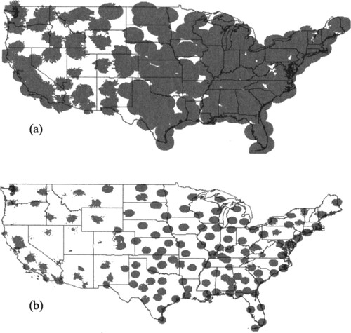
One must also know the distribution of hydrometeor sizes within the radar volume, which can vary significantly depending on the type of precipitation (e. g. continental rain, tropical rain, drizzle, convective rain, stratiform rain, wet snow, dry snow, etc.). In addition, the radar volume must be as close to the surface as possible. In mountain areas, radar estimation of precipitation may be hampered by beam blockage. In this case, special radars must be located in valleys. Radar radiation does not trace a straight path, but rather is bent, owing to refraction associated with gradients in temperature and moisture. Radars are therefore most useful for probing low altitudes relatively near the radar, but at far ranges may reach a minimum in height (radar horizon) as much as halfway to the tropopause. So, when the radar is a long distance from the precipitation, the precipitation near the ground is also not detected (). For Doppler radars, which can detect tornadoes and strong straight-line winds (see Section 4.b.d.ii), tornadoes and strong winds in general also cannot be detected at the surface at long range.

Fig. 5 NEXRAD/WSR88-D coverage at (a) 3 and (b) 1 km AGL at the centre of the beam at 0.5 deg elevation angle. Note how the coverage gets lower as the height above the ground decreases. While coverage is very good at midlevels over much of the U. S. east of the Rocky Mountains, it is much sparser in the boundary layer. (from McLaughlin et al., Citation2009).

The strength of the backscattered radar signal divided by the strength of the transmitted signal is typically given in dB, which is 10 times the logarithm of the power ratio. Since radars must detect a wide dynamic range of signal intensities, it is useful to account logarithmically for the large variation in signal intensity due to the wide range of precipitation reflectivity. Radar reflectivity is commonly given in dBm as the received power ratio relative to one milliwatt. Accounting for distance to the radar, radar reflectivity factor (Z) is given by the sum of all the sixth power of all the scatterers within a cubic metre of volume. Ten times the logarithm of Z divided by the Z of a raindrop of 1 mm in diameter, in a volume of 1 m³, dBZ, is the most useful and widely used measurement of the intensity of the backscattered signal because it is independent of range and provides a useful standard for comparison among different radars.

There have been many empirical studies relating radar reflectivity to precipitation rate (e.g. Anagoustou & Krajewski, Citation1999; Austin, Citation1987) and doing so is still a topic of extensive research. Estimating precipitation rates is critical for warnings and studies of flooding hazards, and for obtaining climate information on precipitation amounts over populated land areas on spatial scales smaller than that of surface observing networks and especially over ocean areas and sparsely populated land areas where there are few if any surface measurements of precipitation. However, one must be cautious in using these radar datasets owing to the many uncertainties inherent in relating radar reflectivity to precipitation rate. When possible, radar estimates of precipitation are calibrated against the available actual measurements from rain gauges at the ground. Range folding must be eliminated, attenuation must be corrected for, and an accurate relationship between radar reflectivity and precipitation rate must be known. Finally, the radar itself must be well calibrated and the radar beam must pass as close to the ground as possible.

ii Doppler radars

Doppler radars compute the line-of-sight component of the wind in a radar volume from the frequency shift of the backscattered signal. There are a number of techniques for doing this including direct calculation of Doppler spectra from a time series of measurements and via “pulse-pair processing.” The former is relatively slow, but delivers the most information (shows the range of velocities within a volume), while the latter is faster and more efficient, but reveals less overall information. The maximum unambiguous Doppler velocity V_max (m s⁻¹) increases with PRF as follows: (3) $V_{m a x} = \pm (λ P R F) / 4,$ (3) where λ is the wavelength of the radar in metres. If the PRF is too small, then there may aliasing, also known as “velocity folding,” which can be corrected objectively using algorithms that compare neighbouring measurements and by assuming that the Doppler velocity varies smoothly in space on the spatial scale the radar can make measurements. Otherwise, multiple PRFs may be needed to resolve the ambiguity. When there is a tornado, for example, the Doppler wind speeds may vary so rapidly that the algorithms may not work well, so that either subjective de-aliasing is necessary or the use of multiple PRFs is employed.

Since both the maximum unambiguous range and Doppler velocities are functions of the PRF, they are both related to each other independently of the PRF as: (4) $R_{m a x} V_{m a x} = (c λ) / 8$ (4) Therefore, there is an inverse relationship, known as the “Doppler dilemma,” between the maximum unambiguous Doppler velocity and the maximum range for a given wavelength, independent of the PRF. Radars must be operated so that range folding is mitigated (radar echoes intense enough to be detected are not present beyond the maximum range) and that Doppler velocities that are aliased can be easily de-aliased. The longer the wavelength, the greater flexibility there is with respect to R_max and V_max, but the larger the antenna must be. Very short-wavelength radars have rather inflexible choices for R_max and V_max, but they are typically limited in range, so that R_max can be sacrificed at the expense of V_max.

There are some research radars, however, that do not send out pulses, but rather send out radiation continuously. These radars have greater sensitivity than pulsed radars, because according to the radar equation the power of backscattered signal increases with pulse length and in this case the pulses are in effect infinitely long, but range information cannot be obtained. Radars that send out radiation continuously while the frequency changes monotonically with time periodically (frequency modulated – continuous wave: FM-CW, or “chirped”) are known as pulse-compression radars, and they can provide range information. They are particularly amenable to space-based radar measurements because they offer high sensitivity at low power output, especially at relatively high frequencies and do not require large antennas. There are, however, some problems unique to pulse-compression radars, which require special techniques to mitigate (Kurdzo et al., Citation2014).

S-band and other UHF (ultra-high frequency) radars, and VHF (very-high frequency) radars, can detect signals from spatial gradients in the index of refraction in “clear” (having no scatterers such as hydrometeors or insects) air through a process known as Bragg scattering, which depends on the scale at which the index of refraction, due to temperature and moisture content, varies in space due to turbulence. Shorter-wavelength radars such as those at C-band, X-band, etc, are not as efficient at producing useful Bragg scattering. “Doppler wind profilers” have therefore been used to measure clear-air wind profiles as a function of height (Balsley & Gage, Citation1982; Gage & Balsley, Citation1978), like rawinsondes, but with much higher temporal resolution (six times to once per hour, depending on the time averaging employed, as opposed to once every 12 h in the operational synoptic network). There are usually several radar beams, each set off a small angle from the vertical,Footnote² so that the horizontal wind may be estimated from the geometric relationship between the angle of the radar beam and the range to the radar volume. For a number of years, a network of wind profilers (Weber et al., Citation1990) maintained by NOAA was operational over the central U.S., but it has since been abandoned for financial reasons. For UHF profilers, when precipitation is present, Rayleigh scattering is assumed instead of Bragg scattering. There is usually a dead zone near the radar for VHF radars, so that wind measurements below ∼ 500 m are not possible (Ecklund et al., Citation1988). Thus, VHF wind profilers cannot usually detect winds in the boundary layer with the desired spatial resolution. The highest the radar can make clear-air, Doppler-wind velocity, measurements depends on the temperature and moisture stratification and is greatest for VHF radars operating at relatively low frequencies.

Surveillance precipitation radars can also estimate the vertical profile of winds using the VAD (velocity azimuth display) technique. This technique works when the winds do not vary substantially over the domain of the radar; in this case, the Doppler velocity should vary systematically as a function of azimuth: When the antenna is pointed in the direction of the wind, the Doppler velocity is at a maximum in approaching velocities, while the Doppler velocity is at a minimum in receding velocities when the antenna is pointed in the opposite direction. The height at which a wind measurement is valid is a function of the range to the radar volume and the elevation angle of the radar beam. VADs, like Doppler wind profilers, are a useful complement to rawinsonde data because they may be collected much more frequently than twice per day. Furthermore, they do double duty because they are also used to detect precipitation. Because they must share the time doing VADs with surveillance scans, they are not available continuously. In addition, there must be sufficient clear-air scatterers, such as insects in the boundary layer, or index-of-refraction gradients so that there can be Bragg scattering when there is clear air.

If the airflow is turbulent, then the range of Doppler velocities within a radar volume can be relatively large. The “spectrum width” is therefore a Doppler-radar variable that may be indicative of turbulence. Also, the vertical shear of the Doppler velocity may also be used as an indicator of turbulence, since high shear contributes to low Richardson numbers, a necessary condition for turbulence.

In order to measure the full, three-dimensional wind field, rather than just the along-the-beam wind component, the Doppler velocity, more than one radar observing volumes from different viewing angles at different locations is required (e.g. Armijo, Citation1969). Bistatic techniques have also been developed which allow one active radar to be paired with one or more fixed-site receivers, each at different locations (e.g. Wurman, Citation1994). There are also techniques for retrieving the three-dimensional wind (SDVR – Single Doppler Velocity Retrieval) by fitting single-Doppler data to dynamic and kinematic constraints (e.g. Liou et al., Citation2018).

iii Polarimetric radars

Most surveillance Doppler radars such as the operational, National Weather Service, S-band radars in the U. S. (Doviak et al., Citation2000) now also have separate vertically and horizontally polarized channels. The relative amount of horizontally to vertically polarized backscattered signal depends on the shape of the scatterers. This effect is measured quantitatively by the differential reflectivity (Z_DR) given as: (5) $Z_{D R} = 10 l o g (Z_{h} / Z_{v}),$ (5) where Z_h and Z_v are the radar reflectivity from the horizontal and vertical channels, respectively. For example, large raindrops that fall are flattened into ellipses, such that the horizontal axis is longer than the vertical axis. The amount of horizontally polarized radiation backscattered is therefore greater than the amount of vertically polarized radiation, so that Z_DR is relatively large. For small raindrops, which are not flattened as much, Z_DR is negligible.

Information about the shape of scatterers is also given by the co-polar cross correlation coefficient (ρ_hv), where (6) $ρ_{h v} = c o r (V_{h h} V_{v v}^{*}) / [| V_{h h} |^{2} | V_{v v} |^{2}]^{1 / 2},$ (6) the normalized correlation (correlation coefficient) of the magnitude of the horizontally-polarized received signals from horizontally-polarized transmitted signals (V_hh) with the magnitude of vertically-polarized received signals from vertically-polarized transmitted signals (V_vv). Hailstones and debris tumble, so that their cross-correlation coefficient is usually low.

The difference in phase between the transmitted and received signals ϕ_DP provides information about the path length of liquid water traversed, since the speed of the radiation is slowed down by the accumulated liquid or solid water substance in its path. More information about the nature of the hydrometeors is given by the rate of change of ϕ_DP with respect to the range from the radar, K_DP, which is known as the specific differential phase. It is useful because changes in phase are not dependent on the calibration of the radar. However, in practice, K_DP can be rather noisy and extreme care must be taken when differentiating ϕ_DP with range.

While Z_DR, ρ_hv, and K_DP are the most commonly used polarimetric variables, there are also others such as the LDR, linear depolarization ratio, and the reader is referred to Zhang (Citation2016) for a discussion of the definition and uses of others. Polarimetric variables have been used to identify hydrometeor/scatterer type using fuzzy logic and also to correct for attenuation. They can be used to estimate drop-size distributions, improve on precipitation estimation based on using radar reflectivity of only one polarization (e.g. Brandes et al., Citation2003), and to determine precipitation-type climatology. More details on the use of polarimetric radar data can be found in Zrnić and Ryzhkov (Citation1999) and Zhang (Citation2016).

The reader is referred to Doviak and Zrnić (Citation2006), Fabry (Citation2015), and Rauber and Nesbitt (Citation2018) for more detailed information on all aspects of radars.

c Other Related Instruments

1 Lidars

Radars that operate at wavelengths near that of light are called lidars (from LIght Detection And Ranging). They detect backscattering from aerosols rather than from larger scatterers such as hydrometeors, etc. Radiation is transmitted as a collimated beam by a telescope. The beams of light are very narrow and can provide information on fine-scale features in clear air. They have been used on the ground at fixed sights, mounted on airborne and ground-based platforms, and on satellites. Some have Doppler capability that allow for wind sensing, particularly in the boundary layer, when there are copious aerosols (e.g. Banta, Citation1995; Bilbro et al., Citation1984; Hardesty et al., Citation1988; McCaul et al., Citation1987).

Raman lidars can remotely measure temperature and water vapour mixing ratio by comparing the backscattered signals from different frequencies, and in the case of water vapour measurements, from different gases. Raman lidars are relatively expensive because they must have high-power transmitters and receive with a large aperture (Weckwerth et al., Citation2016). They have been used at some Atmospheric Radiation Measurement (ARM) sites. DIfferential Absorption Lidars (DIAL) (Turner & Goldsmith, Citation1999), on the other hand, are less expensive and have also been used during a number of field campaigns to measure water vapour. They make use of the amount of attenuation that should occur given the amount of water vapour in the atmosphere, with one frequency used in the centre of that absorbed by water vapour and the other, for comparison, in a wing of the absorption band. DIALs are currently maintained by NCAR, NASA, DOE, and DLR (German Aerospace Center – Deutsches Zentrum für Luft- um Raumfahrt), to name just some organizations. High Spectral Resolution Lidars (HSRLs) have been used to measure aerosols by NASA, DOE, and NCAR, aboard aircraft, as has LEANDRE by the French (Bruneau et al., Citation2001) for water vapour.

2 Sodars

Sodars (from SOund Detection And Ranging) transmit sound waves rather than radiation (Little, Citation1969). The instrument measures the Doppler shift in backscattered acoustic signals (caused by small wind and temperature fluctuations) that are carried by the wind. Depending on the wind speed and width of the receiver, wind profiles are obtained up to several hundred metres; thus, they are primarily used for boundary-layer wind profiling.

3 Observations for planetary and synoptic scales

a Temperature and Moisture

1 Satellite observations

i Temperature and moisture soundings

Atmospheric sounding of the vertical temperature and moisture structure of the atmosphere is one of the key contributions to NWP from meteorological satellites (Menzel et al., Citation2018). The infrared and microwave sounder radiances assimilated into NWP provide complementary information in clear and cloudy atmospheres because clouds are opaque in the infrared part of the spectrum and largely transparent at microwave frequencies. Operating them together makes it possible to cover a broader range of weather conditions. GPS Radio Occultation (GPSRO) observations are complementary to the temperature and moisture measurements retrieved from infrared and microwave radiances observed by the constellation of atmospheric sounders.

The JPSS Cross Track Infrared Sounder (CrIS) and Advanced Technology Microwave Sounder (ATMS) provide temperature, moisture, and trace gas measurements of the atmosphere, with the Ozone Monitoring and Profiler Suite (OMPS), and an earth radiation budget instrument completing the suite of weather instruments on JPSS. The CrIS is an infrared Michelson Fourier Transform Spectrometer (FTS) covering the spectral range of approximately 3.9 microns to 15.4 microns (650–2550 cm⁻¹) with 1305 channels across a swath width of 2200 km. The hyperspectral high resolution and wavelength coverage of CrIS enables the derivation of temperature and water vapour profiles with a horizontal resolution of 14 km and vertical resolution of 1–2 km in the troposphere, and 3–5 km in the stratosphere. The Atmospheric Infrared Sounder (AIRS) on the NASA Earth Observing System Aqua mission, launched in 2002 and still in operation, was a pathfinder that first demonstrated the value of hyperspectral IR soundings. AIRS is a grating spectrometer covering a spectral range from 649 to 2674 cm⁻¹. CrIS continues the AIRS data record with data used in numerical weather prediction models to forecast high impact weather days in advance.

The ATMS on Suomi-NPP and JPSS (NOAA 20) is the latest 22-channel cross-track scanning radiometer measuring microwave radiances from 22 to 183 kHz across a swath width of 2600 km. Temperature profiles are retrieved from the surface to 40 km altitude with a vertical resolution of 3–6 km. Water vapour profiles are retrieved from the surface to 10 km also at a vertical resolution of 3–6 km. An Advanced Microwave Sounding Unit (AMSU-A, B) radiometer is carried on the NOAA-15 to NOAA-19 satellites and on the MetOp-A and MetOp-B satellites. AMSU-A has 15 channels covering a spectral range of 15.8–57 GHz for temperature soundings with 50 km nadir resolution. AMSU-B has 5 channels covering a spectral range from 89 to 183 GHz with 16 km nadir resolution for moisture soundings. A 24 channel Special Sensor Microwave Imager/Sounder carried on the Defense Meteorological Satellite Program (DMSP) F16-19 satellite series provided atmospheric temperature and moisture soundings, as well as land and ocean measurements covering a spectral range from 19.4 to 183 GHz (https://nsidc.org/ancillary-pages/smmr-ssmi-ssmis-sensors). Observations from microwave instruments (ATMS, AMSU-A, AMSU-B), and high spectral resolution infrared instruments such as JPSS CrIS and MetOp IASI (Infrared Atmospheric Sounding Interferometer, Klaes et al., Citation2021) have been shown to have the largest impact of any observation type for reducing medium weather forecasting errors (Joo et al., Citation2013). IASI has high spectral sampling of 0.25 cm⁻¹ and spectral resolution of 0.5 cm⁻¹ over a continuous spectral range from 645 to 2760 cm⁻¹ (3.62–15.5 μm), which provides a comparable or better retrieval than CrIS of atmospheric vertical temperature and moisture structure within its 12 km instantaneous nadir field of view. The combined CrIS/ATMS profiles are useful in nowcasting applications for detecting regions of atmospheric instability and potential outbreaks of severe weather (Esmaili et al., Citation2020). ATMS will extend the time series data on mean global upper air temperatures that began with its predecessor Microwave Sounding Unit (MSU) over twenty years ago. ATMS will also provide global precipitation-rate retrievals for rain and snow with ∼15 km resolution near nadir when combined with CrIS and 35 km resolution stand alone.

ii GPS radio occultation

GPS radio occultation (GPSRO) is an important satellite measurement made from the Constellation Observing System for Meteorology, Ionosphere and Climate (COSMIC-2), consisting of six satellites in LEO (). GPSRO temperature and moisture profiles are widely used in NWP data assimilation. The highly precise radio occultation (RO) signal measured by Global Navigation Satellite System (GNSS) receivers on the COSMIC satellites record the radio signal amplitude and phase in terms of the transit time, which is affected by the density of the air and the amount of moisture within it. The path of a radio signal propagating between a GPS satellite and a receiver on a LEO satellite is bent as a result of refractive index gradients in the atmosphere. The vertical atmospheric profiles of temperature, humidity and pressure are derived by measuring the degree to which GPS signals bend as they travel through Earth’s atmosphere. As a result, upper-tropospheric to lower-stratospheric temperature profiles and lower-tropospheric humidity profiles can be precisely obtained.

2 Radiosonde network

Measurements of the atmosphere above the ground (soundings) began by using kites and balloons in the eighteenth and nineth centuries, and, by the early twentieth century, small networks of these systems (and aircraft) began making routine tropospheric observations. However, it was the invention of the balloon-borne radiosonde (with its radio-transmitting capability) in the 1930s that enabled the first systematic measurements of the global upper atmosphere. The global radiosonde network grew during the 1940s and 50’s, with simultaneous (synoptic) measurements made at 00 and 12 UTC, and occasionally at 06 and 18 UTC. The number of global “raob” stations grew to over 1200 but has diminished to fewer than 800 by 2021, with about 15% of these only launching once per day. A map of the raob observations currently used at the ECMWF is at https://www.ecmwf.int/en/forecasts/charts/monitoring/dcover?facets=undefined&time=2021040712,0,2021040712&obs=Temp&Flag=used; see also Ingleby et al. (Citation2016) for additional issues with the global radiosonde network. The lightweight radiosonde instrument package, ascending at a rate of 5 m s⁻¹, measures temperature, moisture and pressure up to altitudes of 1–10 hPa, where the balloon bursts. The height of each measurement can be deduced from the temperature and pressure using the hypsometric equation. While the number of observations from the network is less than .01% of those from satellites, its global distribution of accurate, high-vertical-resolution and co-located wind and thermodynamic soundings still enable it to rank 6th in importance among 35 global observation systems as determined by forecast sensitivity to observation impact (FSOI) experiments by the Met Office (Cotton & Eyre, Citation2019). A history of the global upper-air network is given by Stickler et al. (Citation2010). Since automated radiosonde systems are becoming more reliable, perhaps the number of raob stations will stop decreasing or increase in future years.

3 Aircraft

Temperature and moisture measurements are made by commercial aircraft on a routine basis, and by research aircraft during field programmes. Over 700,000 automated observations per day (before the 2020–21 pandemic) are obtained from the worldwide Aircraft Meteorological Data Relay (AMDAR) system, which uses existing aircraft sensor, computer and communication systems to transmit meteorological data to ground stations via satellite or radio links (https://public.wmo.int/en/programmes/global-observing-system/amdar-observing-system). The U.S. component of AMDAR is the Meteorological Data Collection and Reporting System (MDCRS), which is funded by the government and its partner airlines; it is also known as the Aircraft Communications Addressing and Reporting System (ACARS). Regional, mid-range airlines that fly in the lower-middle troposphere also transmit weather data, including relative humidity, via the Tropospheric Airborne Meteorological Data Reporting (TAMDAR) system operated by FLYHT, Inc. We note here that data counts for these and all real-time observing systems can be found at https://www.nco.ncep.noaa.gov/pmb/nwprod/gdas/ Although primarily single-level data (they do provide vertical structure during takeoff and landing), their volume makes them an important contributor to the global observation system (4th in Cotton & Eyre, Citation2019). In addition, sounding data over the oceans are enabled by aircraft that can deploy dropsondes, instrument packages that provide thermodynamic information similar to radiosondes. Descending by parachute, they can also be tracked by GPS to provide winds. Dropsondes are frequently deployed by tropical cyclone surveillance aircraft flying in the middle and upper troposphere, and provide crucial information about cyclone structure and its nearby environment. These observations, when assimilated into numerical models, are known to increase hurricane forecast skill (Aberson & Franklin, Citation1999).

4 Other thermodynamic sounding systems

There are many other in-situ and ground-based sensing systems that can provide thermodynamic profile information, most of them currently used for research or local monitoring purposes. Since networks of these systems are not yet on the global scale, we will discuss them in more detail in Section 4.d.

b Winds

1 Satellite

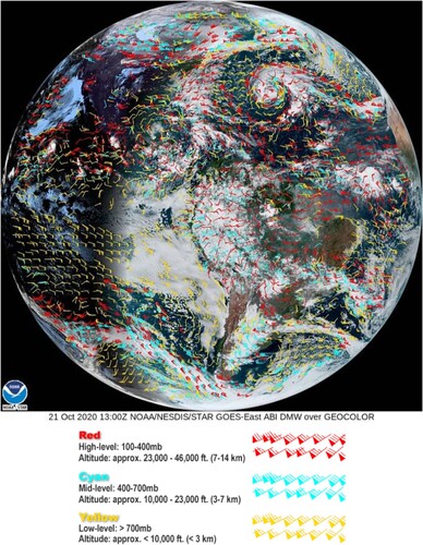
The GEO cloud/moisture derived atmospheric motion vectors () are widely used in global NWP to fill gaps in the global radiosonde network. Information about winds at different levels, areas of wind shear, or jet maxima can be identified by tracking cloud and water vapour features in geostationary and polar imagery sequences. Wind vectors are computed using both visible and infrared spectral bands (https://www.star.nesdis.noaa.gov/GOES/documents/QuickGuide_BaselineDerivedMotionWinds.pdf). Vector heights are assigned in a two-step process. The first utilizes the measured radiances of the target and is based on the spectral response function of the individual satellite and channel being sampled. The brightness temperature of the target is derived from this radiance measurement. Once determined, the brightness temperature is compared with a collocated numerical model guess temperature profile, from which an initial height is estimated. The final vector height is derived in the post-processing of the vector field (see http://cimss.ssec.wisc.edu/iwwg/iwwg.html).

Fig. 6 Derived Motion Wind Vectors (DMW) from the GOES East (GOES-16) Advanced Baseline Imager overlaid on a GeoColor false colour RGB image (Miller et al., Citation2020) at 13 UTC on 21 October, 2020. At this time Category 1 Hurricane Epsilon in the north-central Atlantic (28.9°N, 58.8°W) has a well-defined cyclonic circulation, minimum pressure of 976 hPA, and maximum sustained winds of 74 kts (85mph). Source: NOAA, NESDIS GOES Imager Viewer.

Recent work has focused on mesoscale winds at temporal scales of 1–5 min using dense optical flow methods for feature tracking of pre-storm moisture gradients, cloud streets and outflow boundaries which can lead to convective initiation and storm updraft intensification (Apke et al., Citation2020). Important properties such as vorticity and divergence can also be derived from the more rapid refresh imagery which will have utility in high impact weather analysis and short-range forecasting (Apke et al., Citation2016).

Direct measurement of the wind with lidar in space has recently become possible with the Aeolus mission (https://www.esa.int/Applications/Observing_the_Earth/Aeolus). Aeolus, launched in 2018, is the first satellite mission to provide global profiles of Earth’s wind in cloud-free air. Short pulses of ultraviolet light from a laser measures the Doppler shift from the small amount of light that is scattered back to the instrument from molecules and particles to deliver vertical profiles of the horizontal speed of the winds in the lowermost 26 km of the atmosphere. Tests at ECMWF show short-range forecasts, particularly in the data sparse southern hemisphere and tropics, can be improved when Aeolus data are assimilated (https://www.ecmwf.int/en/about/media-centre/news/2019/tests-show-positive-impact-new-aeolus-wind-data-forecasts).

2 Rawinsondes

A radiosonde balloon that is tracked to provide upper-air wind speed and direction is called a rawinsonde. At first, optical theodolites were used for tracking, which limited wind information to cloud base heights, but these were soon replaced by radio theodolites and radar tracking. This permitted soundings into the stratosphere except when high winds were overhead, creating elevation angles too low to permit tracking. Radio navigation systems used by the aviation industry such as LORAN (LOng RAnge Navigation) and Omega were subsequently used, but have now been replaced by global navigation satellite systems such as the Global Positioning System (GPS), which permits the transmission of very high vertical resolution data at all levels.

A small number of wind observations per day are made by balloons without radiosonde instruments; these are called pilot balloons and are tracked by theodolites.

3 Aircraft

The commercial aircraft observations discussed in Section 3.a.3 usually contain wind speed and direction information. Wind observations from aircraft are calculated from the difference between the velocity of the aircraft with respect to the earth and the aircraft velocity with respect to the air (true airspeed). These velocities are obtained from data from the aircraft navigation system, which includes an inertial platform, magnetic compass and GPS, and its airspeed system, involving pitot static pressure and air temperature (WMO, Citation2018). In principle, these are 3D velocities, but since the vertical wind speed is typically three orders of magnitude less than the horizontal speed, the vertical component is negligible. Winds can also be obtained from navigation information on unmanned aerial systems (UAS) but since these are not yet global in scope, we discuss them in Section 4.d.1.

c Atmospheric Composition from Satellites

Atmospheric composition is important to understand or characterize climate forcing, atmospheric ozone, aerosols, solar effects, air quality, and surface emissions of radiatively and chemically active source gases and particulates. The most important trace gases in the atmosphere are greenhouse gases, which mainly include water vapour (H₂O), ozone (O₃), carbon dioxide (CO₂), nitrous oxide (N₂O), and methane (CH₄). These greenhouse gases warm the atmosphere by absorbing infrared radiation from the surface and shortwave radiation from the Sun, which maintains the earth's temperature. Ozone in the stratosphere absorbs ultraviolet radiation from the sun to protect life on Earth, which makes monitoring and protecting the stratospheric ozone layer extremely important.

Satellite-borne ultraviolet, visible, near infrared (UV/VIS/NIR) spectrometers, nadir and limb-viewing in LEO, are used to retrieve ozone, trace gases, and aerosols (). Tropospheric trace gas, aerosol, and cloud measurements in GEO offer the temporal and spatial sampling to resolve diurnal cycles in emissions, chemistry, and radiative forcing, monitor pollution at urban scales, and observe the inflow and outflow of pollution (Chance et al., Citation2013; NOAA, Citation2020). Atmospheric composition will continue to be a fundamental measurement with the GEO-Ring (https://cpaess.ucar.edu/meetings/2021/noaa-geoxo-atmospheric-composition-town-hall).

Measurements of solar radiation backscattered from the earth (200–400 nm) have a long history, with more recent instruments having hyperspectral capability and extended spectral range to measure boundary layer gases such as SO₂, HCHO (formaldehyde), BrO (bromine monoxide), and NO₂ (see review by Ackerman et al., Citation2019). Visible-Short-Wave Infrared (SWIR) imaging spectrometers typically measure between 380 and about 2500 nm with between 5 and 10 nm spectral resolution (Ayasse et al., Citation2019). These imaging spectrometers are sensitive to gas absorption features, which allows for the detection and quantitative mapping of methane, carbon dioxide, and water vapour.

The Ozone Monitoring and Profiler Suite (OMPS) consist of three spectrometers: a nadir column spectrometer, a nadir profile spectrometer, and a limb sensor. The limb sensor is currently on Suomi-National Polar-orbiting Partnership (S-NPP), though not on NOAA 20 (JPSS-1) but still planned for JPSS-2. The nadir instrument measures dispersed backscattered solar UV radiation to determine ozone profile concentrations and total column amounts. The limb instrument measures limb-scattered solar radiation to determine ozone profiles. The OMPS Nadir Mapper and Nadir Profiler measurements are used to create daily global total ozone data used in monitoring the ozone hole and for UV index forecasts, which alerts the public on the potential of dangerous UV exposure that can lead to skin cancer. OMPS Nadir also provides aerosol and sulfur dioxide (SO₂) indices used for air quality and volcanic eruption warnings. Ozone profiles are assimilated in weather forecast models, and ozone gradients provide improved information on atmospheric circulation. The OMPS limb profiler provides measurements for high-vertical-resolution ozone profiles retrievals; a key data set for monitoring the recovering of ozone due to the elimination of chlorofluorocarbons (CFCs). The OMPS Nadir Mapper has 50 km spatial resolution in its 2600 km swath, the Nadir Profiler has 250 km spatial resolution with 8 km vertical resolution, and the OMPS Limb has a 3 km vertical resolution.

The Ozone Monitoring Instrument (OMI) is a visual and ultraviolet spectrometer aboard the NASA Aura spacecraft. OMI can distinguish between aerosol types, such as smoke, dust, and sulfates, and can measure cloud pressure and coverage, which provide data to derive tropospheric ozone. Its successor, the TROPOspheric Monitoring Instrument (TROPOMI) on the ESA Sentinel-5 Precursor mission has a pushbroom imager design similar to OMI, but with improved spatial resolution (7 × 7 km²), improved sensitivity, and more spectral channels covering the UVVIS-NIR-SWIR spectral range of 270–500 nm, 675–775 nm, 2305–2385 nm (Van Geffen et al., Citation2020).

TROPOMI and OMI have been used to monitor the dramatic impact of the COVID-19 on NO₂ pollution (Bauwens et al., Citation2020). NASA, ESA, and JAXA developed a COVID Dashboard for monitoring the impact of COVID on pollution (see COVID link at https://earthdata.nasa.gov).

The JAXA Greenhouse gases Observing SATellite (GOSAT) and NASA Orbiting Carbon Observatory (OCO-2/3) satellites observe sunlight reflected from Earth’s surface to retrieve atmospheric carbon dioxide (CO₂) concentrations, but use different spectrometer technologies, observing geometries, and ground track repeat cycles. The Orbiting Carbon Observatory-3 (OCO-3) was deployed to the International Space Station in May, 2019. It is technically a single instrument, almost identical to OCO-2.

The Orbiting Carbon Observatory is the first NASA mission designed to collect space-based measurements of atmospheric carbon dioxide with the precision, resolution, and coverage needed to characterize the processes controlling its buildup in the atmosphere. OCO-3 incorporates three high-resolution spectrometers that make coincident measurements of reflected sunlight in the near-infrared CO2 near 1.61 and 2.06 micrometers, and in the molecular oxygen (O2) A-Band at 0.76 micrometers. The three spectrometers have different characteristics and are calibrated independently.

d Radiation Budget

The energy received, reflected, absorbed, and emitted are the components of the Earth's radiation budget. The radiation budget is the balance between incoming solar radiation and outgoing radiation, which is partly reflected solar radiation and partly radiation emitted from the Earth, including the atmosphere. Incoming ultraviolet, visible, and a limited portion of infrared energy (together referred to as “shortwave radiation”) from the Sun drive the Earth's climate system. Some of this incoming radiation is reflected off clouds, some is absorbed by the atmosphere, and some passes through to the Earth's surface, where it may be absorbed or reflected by soil, vegetation, snow, and ice. Larger aerosol particles in the atmosphere interact with and absorb some of the radiation, causing the atmosphere to warm. The heat generated by this absorption is emitted as longwave infrared radiation, some of which radiates out into space.

The gases, ash, and dust particles lofted into the atmosphere during volcanic eruptions may have a profound impact on the climate. These particles cool the planet by blocking the incoming solar radiation and may even circle the Earth with the cooling effect lasting for months to years depending on the characteristics of the eruption as was the case with the catastrophic 1991 eruption of Mount Pinatubo in the Philippines (Robock, Citation2002).

The radiation budget is measured by Clouds and the Earth’s Radiant Energy System (CERES). CERES on S-NPP and JPSS provides continuity of the CERES instrument on the NASA EOS AQUA satellite and extends the climate data record of Earth’s radiation budget from the first Earth Radiation Budget Experiment (ERBE) (Wielicki et al., Citation1996). CERES is a scanning radiometer system with total shortwave and longwave window channels with a 20 km footprint at nadir. CERES products include both solar-reflected and Earth-emitted radiation from the top of the atmosphere to the Earth’s surface. Cloud properties are determined using simultaneous measurements from VIIRS.

e Surface Measurements

The first atmospheric measurements were made at the surface, beginning with qualitative assessments of wind, temperature, moisture and precipitation, followed by quantitative observations as instruments to measure these quantities were invented in the sixteenth and seventeenth centuries. The barometer was also invented during this period, often used in “Lagrangian mode” by scientists ascending hills to deduce that pressure decreased with altitude. Networks of surface instruments that enabled the discovery of two-dimensional surface weather patterns began in modest fashion in the eighteenth century, but the real-time use of such “synoptic” observations could not occur until the invention of the telegraph in the mid-nineteenth century. There is a history of atmospheric observations in Lin, 2022, and a slightly larger overview by Stith et al., Citation2019. Many books on instrumentation exist, beginning with Middleton and Spilhaus (Citation1953) classic work, textbooks such as Brock and Richardson (Citation2001), Emeis (Citation2010), and Harrison (Citation2015), online COMET material at https://www.meted.ucar.edu/education_training/course/58, and a recent handbook, Foken (Citation2021).

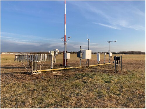
We start with the variables shown on a standard surface station plot as shown in . Temperature is observed by a variety of thermometers – see above instrument texts for the many measurement techniques. Pressure is provided by a barometer – early versions were mercury based but most now are of the aneroid type. The actual station pressure measured is not usually shown – its value is reduced to sea level by hypsometric methods (Bluestein, Citation1992), which permits construction of surface pressure charts. The 3-hour pressure tendency is also indicated. Wind speeds are measured by anemometers, which usually contain wind vanes to provide wind direction. Among the many types of wind instruments (see referenced texts), the most precise one is the sonic anemometer, which is often used for turbulence measurements. It measures the individual components of the wind (u,v,w) by transmitting sound pulses in opposite directions along three orthogonal paths. Since sound waves travel with the atmospheric medium, a wind component can be obtained by the difference between the two transit times. The temperature can also be calculated by the sum of the two transit times using the speed of sound equation. By convention, most surface stations measure wind at 10 m, with all other variables measured 1.5–2 m above the ground. shows a typical U.S. Automated Surface Observing System, which measures most of the 18 weather elements shown in .

Fig. 7 Surface station plotting model (https://en.wikipedia.org/wiki/Station_model#/media/File:Station_model.gif).

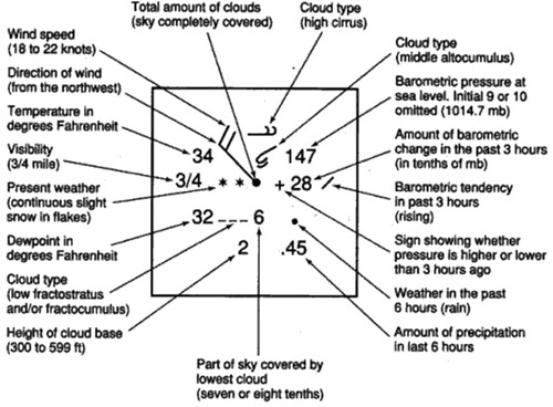
Fig. 8 Typical Automated Surface Observing System (ASOS). Courtesy of Kenneth Boutin, National Weather Service.

The moisture content of the air is expressed in surface reports as the dewpoint temperature, which can be measured in combination with the temperature via a chilled-mirror hygrothermometer. The general term hygrometer refers to any instrument that measures water vapour content, but there are many kinds, depending on the variable desired and the physical principle being used to make the measurement. For example, absorption hygrometers and carbon hygristors (often used in radiosondes) measure relative humidity directly, psychrometers measure wet bulb temperature and dewpoint hygrometers measure dewpoint temperature. There are a variety of other moisture variables important to atmospheric scientists such as specific humidity, mixing ratio, water vapour pressure, saturation vapour pressure, and these can be obtained from the moisture variable that is measured (along with temperature and pressure) via thermodynamic formulas (e.g. see Bohren & Albrecht, Citation1998)

Current weather specification is based on the familiar WMO 99 weather types chart (http://craigsweb.net/mystuff/WxSymbols.gif) and was originally provided by human observers. With the advent of automated observations, present weather identification became much more difficult (note that a select number of stations still use human observers for weather). For example, the U.S. ASOS stations (from ASOS Users Guide: https://www.weather.gov/media/asos/aum-toc.pdf), does have precipitation identification instrumentation to distinguish between rain and snow, which also determines the intensity (light, moderate, heavy). There is a freezing rain sensor known as a “magnetostrictive oscillator”, which is also found on aircraft to detect icing. Lightning detection information is provided by the private sector, which has deployed lightning detection networks worldwide (see Section 4.c). Rain gauges provide precipitation totals, including frozen precipitation if the gauge is heated. Common gauge types include tipping bucket, weighing, capacitance, disdrometer, acoustical and optical (Nystuen, Citation1999; Nystuen et al., Citation1996). The latter can also provide the type and intensity of precipitation. Disdrometers are used to determine the dropsize distribution of rain. Hailpads and momentum-detecting steel spheres are used to obtain the size distribution and mass of hailstones. We note that there is a volunteer effort to collect daily rain, hail and snow reports known as the Community Collaborative Rain, Hail and Snow Network (CoCoRaHS) – see https://www.cocorahs.org.

Snow measurements, especially of seasonal high-elevation snowpacks, are vital for water management applications. Snow depth is reported at some surface stations by human observers but not by most automated stations. However, thousands of sites in, e.g. the western U.S. exist to provide snow depth and snow water equivalent (SWE) information. Some sites, or snow courses, are monitored manually via periodic visits to measure depth and SWE using snow tubes. An automated network, SNOTEL (https://www.wcc.nrcs.usda.gov/snow/), records hourly information on SWE (measured by the weight of snow on a snow pillow), snow depth (measured by transit times of ultrasonic pulses to snow surface and back), and other standard meteorological variables. The data are transmitted by radio signals, cell networks or via satellite. Simple snow stakes are frequently used and can be monitored manually, via camera, or, if in remote regions, by aircraft or satellite (if telemetered).

Although a full treatment of hydrologic measurements is beyond the scope of this paper, what happens after the rain falls and the snow melts is extremely important to monitor because of the subsequent threats of flash flooding and main stem flooding (and droughts in the case of insufficient water). First, a real-time multi-sensor (rain gauges, radar and satellite estimates) analysis is needed to assess current rainfall rates – in the U.S. this is provided by NOAA’s Multiple Radar Multiple Sensor (MRMS) system (https://www.nssl.noaa.gov/projects/mrms/) on a 1 km grid every 2 min. The surface runoff and subsequent river levels are measured by over 8000 stream gauges operated by the U.S. Geologic Survey and Army Corps of Engineers. These inputs, plus outflow data from over 5000 reservoirs and quantitative precipitation forecasts from operational models, provide initial conditions for National Water Model (https://water.noaa.gov/about/nwm) streamflow forecasts at 2.7 million river locations every hour.

Two variables very important to aviation – ceiling and visibility – are also provided by human observers or automated sensors. A common instrument to detect ceilings is a laser beam ceilometer, which, because it transmits vertical, intense pulses of visible or near-infrared light, operates using lidar principles. Its range is typically 3–4 km, so high clouds are not detected; also, it cannot report 2–3 levels of clouds as human observers do. In principle, the thousands of ceilometers deployed at airports around the world could provide high-resolution time-height profiles of backscattered intensity that would provide useful PBL structure information; – this is now commonly done in Europe but not yet in the U.S. Cloud cover information (in %) is determined from ceilometers by analyzing the “cloud hit” information for 30–60 min. Whole- or all-sky cameras are also used to observe fractional cloud coverage. Types of clouds are reported by human observers but not by instruments, although lightning sensors indicate the presence of convective clouds. Visibility, which is easy to report by observers looking at objects of known distance, is challenging to automate (see ASOS Users Guide referenced above). A common method is to measure the extinction coefficient of the atmosphere (from light scattering) with a telephotometer or transmissometer and relate it to “runway visual range”. The need to report specific types of obscurations such as fog, mist, freezing fog and haze is accomplished by ASOS by combining information from the visibility, temperature, dewpoint and present weather sensors. Cameras are also used for monitoring visibility, especially where fog and smoke may be common.

Land surface measurements are vital to assess the regional climate but are also important for mesoscale and storm-scale weather prediction (Lanicci et al., Citation1987). The temperature of the land surface (skin temperature) is rarely measured in situ but is sensed by satellites as the radiative temperature of the earth’s surface. Soil temperature measurements are made at depths varying from 5 to 100 cm, under both bare and vegetated soil using buried thermistors or thermocouples, and are especially important to the agricultural community. Soil moisture information is crucial for hydrological, agricultural, fire weather and other interests, and is most useful if, like temperature, a profile at 2–4 levels is obtained so that vertical fluxes can be estimated. It is a challenging measurement, not commonly obtained at standard surface stations, but is measured, e.g. at over 100 stations by the Oklahoma Mesonet (Illston et al., Citation2008). A heat dissipation sensor is used that measures the change in soil temperature after a heat pulse is introduced – this change is proportional to soil moisture. Several variables in additional to soil water content can be estimated such as soil water tension (or soil water potential) and fractional water index. Other methods to measure soil moisture include gravimetric sampling, tensiometers and neutron scattering. Areal measures are provided by the cosmic ray soil moisture sensor (400 m scale), passive microwave radiometry from satellites and gravitational anomalies from the GRACE satellite (Sadeghi et al., Citation2020). A major effort has been made in the U.S. to collect soil moisture data from over 20 sources – see http://nationalsoilmoisture.com – a true “network of networks.”

The local surface energy balance requires several additional measurements: net radiation (downward and upward shortwave and longwave radiation), sensible and latent heat fluxes, and heat conduction. The radiation measurements (and instrument used) made at the surface to determine the balance include direct solar radiation (pyheliometer), global radiation – solar plus diffuse sky radiation – (pyranometer), terrestrial radiation (pyrgeometer), and albedo (albedometer). It is also possible to measure specific wavelengths such as ultraviolet radiation (dosimeter) and infrared radiation (spectrometer, radiometer, interferometer). Heat and moisture (and momentum) fluxes require profiles of temperature, moisture and wind, using instruments already mentioned. Using these observations, the surface energy balance can be monitored, as well as (with the help of satellite data) useful quantities such as the Bowen ratio, Normalized Difference Vegetation Index (NDVI), and other properties of the soil and canopy.

The surface layer is quite turbulent, requiring high spatiotemporal measurement resolution and accurate instrumentation; see Foken (Citation2017) for a detailed description of such measurements.

The measurement of atmospheric aerosols and pollutants, originally very important in urban areas for assessing health impacts, is also important for knowledge of total radiative forcing affecting climate change, and for providing warnings to people worldwide affected by wildfire smoke. Pollutants, by definition, are substances that, for the most part, do not occur naturally in the atmosphere, or, if they do, are enhanced to hazardous levels (e.g. O₃ near the surface) . The AMS online Glossary (https://glossary.ametsoc.org/wiki/Welcome) summarizes U.S. EPA definitions of “criteria pollutants”, that can injure health or harm the environment and “toxic pollutants” that are specifically known to cause cancer or other serious health problems. The criteria pollutants are carbon monoxide, lead, nitrogen dioxide, ozone, particulate matter with size ≤10 μm (PM-10) and sulfur dioxide. These quantities are monitored and regulated by the EPA, and public warnings are issued if levels become especially dangerous. The EPA has identified at least 188 toxic pollutants which are monitored at the source of emission (such as at chemical plants and refineries), with regulations requiring reduction or elimination of these air toxins.Footnote³ We note that there are hundreds of air quality monitoring networks that measure criteria pollutants and many other hazardous gases or particles; – many are listed in the National Academy of Sciences (NAS) “Network of Networks” study (NRC, Citation2009; see Table B.2).

Aerosols are defined as colloidal systems wherein the “dispersed phase” is either solid or liquid particles and the “dispersion medium” is gas (here, the atmosphere) (AMS online Glossary – https://glossary.ametsoc.org/wiki/Welcome). Atmospheric conditions such as fog, smoke, smog, mist and haze are considered aerosols, although haze may also contain photochemical smog (O₃, NO_X, hydrocarbons). They all cause obscurations to visibility, endangering aviation and transportation operations in general, whose measurement is described above. Smoke, comprised of small particulate matter caused by combustion, also causes obscurations as well as health hazards. The increase in wildfires and acreage burned in recent years has brought greater attention to “fire weather”, for which it is important to monitor and predict precipitation trends, temperature, soil moisture or “wetness”, fuel availability and dryness, and wind speed. Cloud condensation nuclei and dust are also aerosols, most of which originate naturally (e.g. from soil, salt spray, smoke, volcanic eruptions, pollen and other organic material). Many of these substances are not regularly measured (unless they affect visibility, health and/or air quality), but are done so during field research experiments, often in aircraft.

Finally, the composition of the atmosphere is monitored from both the surface and space, the latter covered in Section 3.c. The two main components, nitrogen and oxygen, are not monitored as closely as the minor constituents or trace gases such as water vapour, carbon dioxide (CO₂), ozone (O₃), methane (CH₄), carbon monoxide (CO), nitrous oxides, etc. since the latter are more important to global radiative forcing, weather and human health. Water vapour is the most important greenhouse gas, as well as the source for the earth’s hydrologic cycle and its measurement is described above; however, its total percentage of the atmosphere’s mass is not changing very quickly. CO₂, on the other hand, has increased over 30% over the past 62 years as seen by the famous Keeling curve from the Mauna Loa site (https://www.esrl.noaa.gov/gmd/ccgg/trends/). Given that the pristine conditions at 3400 m on Mauna Loa might not be representative of other locations, NOAA has been monitoring CO₂ at many other sites around the globe (https://www.esrl.noaa.gov/gmd/ccgg/about.html), with similar trends observed. Spectroscopy methods are used to make the measurement, e.g. via a non-dispersive infrared analyzer or cavity ring-down spectroscopy (https://www.esrl.noaa.gov/gmd/ccgg/about/co2_measurements.html). Air samples are either pumped directly into the instrument, or, if not at a reference network site, are collected in flasks and brought to a laboratory. Great care is taken to collect representative, unpolluted samples at many sites world-wide, both on the ground and via aircraft flights. Most of the world’s laboratories that measure CO₂ also measure the other atmospheric gases mentioned above, but the details of these measurements are beyond the scope of this paper.

We close this section by noting that monitoring the earth’s surface climate and its variability requires a network of long-term, appropriately sited and well-instrumented stations around the globe. A NAS study on the “Adequacy of Climate Observing Systems” states the case for the importance of such networks (NRC, Citation1999). The various Federal and private sector networks for weather monitoring are not well suited for this task because of their large variability in siting, measurements taken and quality. The U.S. has joined with the WMO to support the Global Climate Observing System (GCOS) by creating the U.S. Climate Reference Network (USCRN). The USCRN is comprised of about 140 sites distributed around the U.S., including at least 23 in Alaska (https://www.ncdc.noaa.gov/crn/overview.html). Each site measures temperature, precipitation, soil moisture and temperature, surface (skin) temperature, solar radiation, wind speed, relative humidity, and wetness (via a disdrometer). The data are recorded every 5 min and transmitted hourly to a geostationary satellite, from which the information is downloaded to the National Center for Environmental Information (NCEI). The U.S. also supports a Cooperative Observer Program (Coop) that is comprised of over 4000 volunteer surface sites that (at minimum) report daily maximum and minimum temperature, snowfall and 24-hr precipitation totals (https://www.weather.gov/coop/Overview), which are also important for monitoring long-term climate change.

4 Observations for mesoscale and convective-scale weather

a Satellites

While the first generations of satellites primarily provided observations on the synoptic and large-mesoscale, recent generations now measure the atmosphere and surface properties at the convective or storm-scale (0.25–5 km). This section will describe the current sounding and imaging capabilities of many of the instruments carried by the satellites shown in .

1 Multispectral imagery

The spectral bands of the satellite imagers cover select bands in the visible and infrared portions of the electromagnetic spectrum. Horizontal spatial resolution in the visible ranges from 250 m (MODIS) – 375 m (VIIRS) in LEO to 500 m in GEO, and the resolution of infrared channels range from 1 km in LEO to 2 km in GEO. The operational imagers in GEO can scan the full earth disk in 10 min, with smaller mesoscale domains sampled every 1–2.5 min. Various channel combinations are used to make additional decision aids and products for forecasting (e.g. fog, smoke, airmass, dust among others). The National Oceanic and Atmospheric Administration (NOAA) Geostationary Operational Environmental Satellite (GOES) and the European Organization for the Exploitation of Meteorological Satellites (EUMETSAT) Meteosat Third Generation (MTG, planned launch in late 2022) geosynchronous satellites also have lightning imagers that provide storm-scale day/night imaging of lightning discharges including their radiant energy, areal extent, and propagation, never before possible from space.

The current Meteosat Second Generation (MSG) 12 spectral channel Spinning Enhanced Visible and Infrared Imager (SEVERI) provides the pathfinder heritage for the newest generation of geostationary satellites and the many derived products used in nowcasting. These products use various combinations of the visible and infrared channels to derive products such as the Convective Rainfall Rate (CRR), Rapidly Developing Thunderstorm (RDT), and a visible/infrared convective storm blended composite called the Sandwich product (http://nwsaf.org; https://cwg.eumetstat.int/).

The new generation 16-band multispectral imagers in the GEO-Ring depicted in (e.g. NOAA GOES ABI, Japanese Meteorological Administration (JMA) Himawari, Korean Meteorological Agency (KMA) GeoKompsat 2a, and EUMETSAT MTG Flexible Combined Imager (FCI)) are a major advancement over the previous generation. Earlier generation 5-band GEO imagers now have 16 bands (3 Visible, 3 Near IR (NIR), 10 Long Wave IR (LWIR)) with spectral coverage from 0.46 to 13.3 µm and with spatial resolutions that range from 500 m (VIS) to 2 km (IR). Similar advancements are found in the new generation of POES multispectral imagers first developed for the Earth Observing System (1999 launch on NASA’s Terra satellite; 2002 launch on NASA’s Aqua satellite). The 36 spectral band Moderate Resolution Imaging Spectroradiometer (MODIS) instruments might be considered the pathfinder for the new generation of operational GEO and LEO imagers. The 22 spectral band Suomi National Polar-orbiting Partnership (S-NPP) and Joint Polar Satellite System (JPSS, Goldberg et al., Citation2018) Visible Infrared Imaging Radiometer Suite (VIIRS) instruments are major advancements over the previous generation Advanced Very High-Resolution Radiometer (AVHRR) 7-band imager on the NOAA (Goldberg et al., Citation2018) polar satellites.

JPSS-1 (now NOAA 20) operates in an early afternoon 1330 local equatorial crossing time sun-synchronous orbit at an altitude of 833 km. The NOAA 20 orbit is separated from the S-NPP by 50 min. The Terra MODIS overpass is at 1030 local while MODIS Aqua is at 1330 local time. These imagers are valuable for land, ocean, and atmosphere monitoring and provide products to support impact-based decision support services. MODIS has spatial resolutions of 250, 500 m, and 1 km depending on the wavelength and spectral coverage of the VIS/NIR/SWIR (0.405–2.155 µm) and the Mid-wave IR (MWIR) to the Long-wave IR (LWIR) (3.66 µm to 14.28 µm). The VIIRS has 22 spectral bands between 0.412 and 12.01 µm covering a swath of 3000 km, including 16 moderate resolution bands with a spatial resolution of 750 m at nadir, 5 imaging resolution bands with spatial resolution of 375 m at nadir, and one panchromatic Day-Night Band (DNB) with 750 m spatial resolution throughout the scan.

Some improvements of VIIRS (launched in 2011 on S-NPP) over MODIS (launched on NASA Terra in 1999) are that the VIIRS has one shortwave and one longwave imaging channel at 375 m resolution compared to 1 km for MODIS, which improves VIIRS ability at these wavelengths to see greater detail. VIIRS pixels only expand minimally toward the edge of scans, providing overall higher resolution. VIIRS has a wider swath than MODIS, 3000 km vs. about 2400 km. Lastly, VIIRS has a Day Night Band (DNB) for nighttime imaging. VIIRS has some disadvantages as well compared to MODIS, perhaps most notably having only 22 channels compared to MODIS’ 36 channels. The most significant shortfall is VIIRS’ lack of water vapour channels at around 7 micrometers, which are used for water vapour-based applications on MODIS (including feature-tracked winds).

2 Atmospheric soundings

The primary contribution of infrared and microwave soundings to mesoscale and high impact weather diagnostics, nowcasting, and short-range forecasting is through their assimilation into NWP models. Near real-time satellite sounding retrievals of temperature and moisture from LEO, available at the right place and time, can also aid in warnings of severe weather through measurements of (evolving) atmospheric stability conditions (Esmaili et al., Citation2020). Such retrievals are useful in providing forecasters with gap-filling data between the standard radiosonde launch times around 00 and 12 UTC.

A much-anticipated advance for atmospheric observations of weather and climate is hyperspectral sounding from geostationary orbit. The GEO surveillance perspective offers significant improvements for nowcasting and very short-range forecasting of high impact environmental phenomena. The capability first demonstrated by the Geostationary Interferometric Infrared Sounder (GIIRS) on the Chinese Fengyun-4A (FY-4A) satellite (Yang et al., Citation2017; https://space.oscar.wmo.int/instruments/view/giirs) will be followed by the European MTG-S Infrared Sounder (IRS). The IRS will be the first hyperspectral IR instrument having longwave infrared spectral coverage of 680–1210 cm⁻¹ (14.3–8.3 μm) with > 800 spectral channels and mid-wave infrared spectral coverage of 1600–2250 cm⁻¹ (6.25–4.6 μm) with > 920 channels on a geostationary satellite providing full-disk coverage with high spatial (4 km at nadir) and temporal (30 min) resolution moisture and temperature profiles of the atmosphere (Holmlund et al., Citation2021). The IRS is based on an imaging Fourier-transform interferometer with a spectral resolution better than 0.754 cm⁻¹ and a spectral sampling of 0.6 cm⁻¹. All interferograms from the IRS are disseminated (downlinked) to ground, where they are transformed into spectra via fast Fourier transformation and are radiometrically and spectrally calibrated and geolocated.

The main objective of the IRS is to provide information on specific humidity and temperature with good vertical resolution either via data assimilation methods or as retrieved profiles, which also drives the baseline scan sequence concept of operations. The use of sequences of IRS data will also enable extracting information on atmospheric flow, either through Derived Motion Winds (see ) or via the wind tracing in four-dimensional variational (4D-Var) data assimilation schemes. A GEO hyperspectral sounder with similar performance to that of IRS, with a planned launch in the 2030s, is also under study by NOAA NESDIS (Maier et al., Citation2021). JMA and KMA are evaluating their prospects for a GEO IRS to fill out the Geo-Ring as recommended by the WIGOS 2040 Vision (WMO, Citation2019). GIIRS and IRS will provide valuable proxy data for the other future GEO sounders as well as opportunities for research.

3 Day/Night Band

A Day/Night band (DNB), previously on the Defense Meteorological Satellite Program (DMSP) satellite series and a more advanced version on the Joint Polar Satellite System (JPSS) Visible Infrared Imaging Radiometer Suite (VIIRS), provides seven orders of magnitude of radiance sensitivity. The DNB is a highly sensitive, calibrated broadband panchromatic channel with 750 m spatial resolution covering the visible to near-infrared wavelengths from 500 to 900 nm (Hillger et al., Citation2013). The DNB is capable of direct detection of city lights and other terrestrial (e.g. fires, gas flares) emission sources with illumination as little as a quarter moonlight, as well as the light reflecting from cloud tops, dust, and pollution. The DNB can also capture images for scenes that are illuminated by nightglow emission. Gravity waves emanating from the overshooting tops of deep thunderstorms with vigorous updrafts have even been observed in the nightglow imagery (Miller et al., Citation2015). Nighttime remote sensing methods traditionally rely on infrared and microwave channels. However, infrared observation of the lower atmosphere may be obscured by upper-level clouds and a lack of thermal contrast, while microwave sensing provides lower spatial and/or temporal coverage, as in passive microwave imaging.

4 RGB imagery

IR images are often colorized, referred to as RGB or red-green–blue imagery, using band combination recipes to bring out details in cloud patterns, aerosols, dust, and air mass properties (dry or moist). A Quick Guide for generating a dust RGB can be found at (http://rammb.cira.colostate.edu/training/visit/quick_guides/Dust_RGB_Quick_Guide.pdf). Infrared imagery, like visible imagery, can be used to analyze thunderstorms (enhanced-v temperature couplets), mid-latitude systems (comma cloud), and hurricanes (eye). Cloud-top temperatures, like surface-feature temperatures, can be determined using IR imagery and reveal the difference between low and high clouds because they have different cloud-top temperatures. Enhancement curves are often applied to IR imagery to highlight tops of thunderstorms.

5 Lightning imaging

Lightning imaging day and night from LEO (Blakeslee et al., Citation2020) with 4 km resolution at nadir (International Space Station Lightning Imaging Sensor, ISS-LIS) and from GEO (Goodman et al., Citation2013; NOAA-NASA, Citation2019) with 8 km resolution at nadir (GOES Geostationary Lightning Mapper (GLM)) use a nadir-pointing high speed (2 milliseconds sampling) camera to detect the optical transient signature of lightning illuminating cloud tops at 777.4 nm, a wavelength associated with the neutral atomic oxygen emission line triplet of the lightning spectrum. The GLM is a recent new capability for mapping total lightning (in-cloud and cloud-to-ground) across the western hemisphere from the GOES-East (75.2W) and GOES-W (137.2W) positions in GEO (Rudlosky & Virts, Citation2021). GLM can uniquely observe the path of a single dangerous discharge originating in the convective storms of a mesoscale convective system (MCS) that propagate into the trailing stratiform region over many hundreds of km (Peterson et al., Citation2020; Rudlosky et al., Citation2020). In 2023 the EUMETSAT MTG Lightning Imager will complement GLM with coverage of Europe, Africa and the adjacent oceanic regions.

6 Microwave precipitation measurements

The Global Precipitation Measurement (GPM) core () has two widely used primary instruments, a Dual-frequency Precipitation Radar (DPR) and a GPM Passive Microwave Imager (GMI). The DPR consists of a Ku-band precipitation radar (KuPR, 13.6 GHz) and a Ka-band precipitation radar (KaPR, 35.5 GHz), both having 5 km spatial resolution at nadir and covering a swath width of 245 km. The DPR is more sensitive than its TRMM predecessor especially in the measurement of light rainfall and snowfall in mid latitude regions. Rain/snow determination is accomplished by using the differential attenuation between the Ku-band and the Ka-band frequencies. The GPM Microwave Imager (GMI) is a multi-channel, conical-scanning, microwave radiometer that enables the core spacecraft to serve as both a precipitation standard and as a radiometric standard for the other GPM international partner constellation satellites (https://gpm.nasa.gov/missions/GPM/GMI). The GMI has thirteen microwave channels ranging in frequency from 10 to 183 GHz. In addition to carrying channels similar to those on the Tropical Rainfall Measuring Mission (TRMM) Microwave Imager (TMI), the GMI carries four high frequency, millimetre-wave, channels near 166 and 183 GHz (https://gpm.nasa.gov/missions/GPM/GMI). The GPM core and its partner passive microwave radiometers, when combined with the GEO imagers, can create a widely-used precipitation product called IMERG (Huffman et al., Citation2018) that is updated every 30 min through temporal morphing of the instantaneous rainfall fields, and that is widely used in nowcasting and NWP validation. An excellent review of precipitation measurements and methods from space is found in Levizzani et al. (Citation2020).

Further information on satellite missions and instruments can be found in the WMO Observing Systems Capability Analysis and Review (OSCAR) database for Space-based Capabilities (OSCAR/Space), updated October 2020 (https://www.wmo-sat.info/oscar/spacecapabilities). The COMET/MetEd satellite training modules offer free registration and provide current information on many of the weather satellites, their instruments, and the use and interpretation of their data (https://www.meted.ucar.edu/training_detail_university.php). In addition to the myriad of on-line resources, three books on weather satellites the reader may also find useful are Kidder and Vonder Haar (Citation1995), Liang (Citation2017), and Goodman et al. (Citation2019). The latter two references are available as eBooks and individual chapters can be purchased or freely downloaded if your library has subscribed to Science Direct access.

7 Snow and ice mapping

The cryosphere broadly includes snow, sea ice, lake and river ice, icebergs, glaciers, ice caps, ice sheets, ice shelves, permafrost, seasonally frozen ground, and solid precipitation. Notable cryosphere-related hazards include blizzards, snow/ice-melt flooding, ice jams and break-up, avalanches, sea-level rise, and climate change. Visible and infrared measurements from the ABI and VIIRS multispectral imagers (Key et al., Citation2013, Citation2019) and passive microwave measurements (Meier et al., Citation2017) from AMSR (Advanced Microwave Scanning Radiometer), AMSR-E, and AMSR-2 provide measurements of precipitation, snow cover, and sea and lake ice surface temperature, concentration, thickness, and motion and other variables of interest for global change science and monitoring. Ice thickness inputs include surface skin temperature, air temperature, radiation fluxes at the surface, snow depth, atmospheric moisture, and wind. The AMSR2, launched in 2012, is still operating and is a successor to AMSR on the Japanese ADEOS-II satellite and AMSR-E on the NASA Aqua satellite. The AMSR-2 covers a 1450 km swath from its orbital altitude of 700 km, collecting daytime and nighttime data over 99% of the Earth every two days.

Synthetic Aperture Radar (SAR) has a long history (see tutorial at https://earth.esa.int/documents/10174/642943/6-LTC2013-SAR-Moreira.pdf) of making active microwave measurements at X-band and C-band for snow cover mapping (Tsai et al., Citation2019) and sea ice classification and charting in the remote arctic regions (Zakhvatkina et al., Citation2019). The SAR is an airborne or satellite-based side-looking radar system which uses the platform motion to electronically simulate a very large antenna aperture to generate high-resolution remote sensing imagery (https://www.radartutorial.eu/20.airborne/ab07.en.html). SAR measurements at C-band are available from ESA’s Sentinel-1 and the Canadian Space Agency RADARSAT. The 3-satellite commercial RADARSAT Constellation Mission (RCM) provides high spatial resolution mapping of snow and ice (as well as marine surveillance, disaster management, and natural resource mapping).

NASA’s Ice, Cloud and land Elevation Satellite (ICESat and ICESat-2) uses a lidar altimeter (GLAS, Geoscience Laser Altimeter System) to measure ice sheet elevation and sea ice thickness. Lidar altimetry has fine horizontal resolution of tens of metres and vertical resolution less than 10 cm that also makes it possible to determine ice thickness and the boundary between sea water and polar ice and (after successive passes) to profile the height along-track in order to map ice thickness (Farrell et al., Citation2020; Lai & Wang, Citation2021). The lidar altimeter requires extremely accurate orbit determination using GPS, since the basic ranging measurement provides the distance of the object from the satellite in orbit. Ice cover and concentration are critical parameters for numerical weather prediction and as climate change indicators(e.g. surface emissivity, energy balance) and for operational ice services such as the NWS Alaska Sea Ice Program (https://www.weather.gov/afc/ice), the NWS National Operational Hydrologic Remote Sensing Center (https://www.nohrsc.noaa.gov/) and the US National Ice Center (https://usicecenter.gov/).

b Radar

1 Operational radars

Weather radars were specifically developed with the purpose of detecting mesoscale and convective-scale precipitation systems because they can quickly scan mesoscale areas, which are difficult to sample sufficiently and quickly enough using in situ sensors mounted on instruments such as rawinsondes or on aircraft. S-band radar systems are best suited for surveillance of mesoscale and convective-scale features. These radars are useful for computing the climatology of precipitation, type of precipitation, and type of precipitating system over broad areas. The range of these S-band surveillance radars is typically 100–200 km or more, but is limited by the sensitivity of the radar, the nature of the scatterers, and the lowest altitude that can be scanned owing to the curvature of the Earth and refraction.

The radar-echo imagery from a network of radars may be composited into a mosaic on a much larger domain to show how precipitation varies across the country. Some composited products of three-dimensional radar structure have become available in the U. S. and are archived (e.g. Homeyer, Citation2014) and are very useful for climate studies. The MRMS programme, mentioned earlier, makes use of composited radar data to produce quantitative precipitation estimates over broad areas (Zhang et al., Citation2016). Radar resolution and the height above the ground are important considerations in producing these composites because the resolution at far ranges from radars is much less than that near radars and beyond a given range, there are no data below a given altitude (). There are also surveillance radar networks in Europe, in Asia, and elsewhere around the globe, but not all are free and open access, especially when the networks are run by the military and the data are considered a security issue.

C-band systems and X-band systems have also been used, the latter particularly in mesoscale networks such as CASA (Collaborative Adaptive Sensing of the Atmosphere) in the U. S. Advantages of CASA-like networks are that the atmosphere can be sampled near the ground () and that high spatial resolution can be attained when viewing small-scale features such as tornadoes (McLaughlin et al., Citation2009).

2 Measurements made by radars

There are many radar measurements unique to the mesoscale and convection scale. These measurements include both non-severe and severe phenomena.

i Non-severe phenomena

Radar can detect the melting level as an enhanced region of reflectivity within stratiform precipitation in extratropical cyclones. It can show the leading convective-line and stratiform regions of precipitation within mesoscale convective systems (MCSs). Mesoscale bands of precipitation are found within extratropical cyclones and along fronts. Precipitation type can be identified from polarimetric-variable information and the important rain – snow transition line can be located.

Fine lines of enhanced reflectivity near the ground, which are caused by the convergence of insects, mark mesoscale zones of convergence (Wilson et al., Citation1994). These fine lines mark boundaries such as gust fronts, outflow boundaries, surface fronts, and sea-breeze/land breeze fronts, and others. When there are sufficient scatterers, Doppler radars show zones of convergence along these features.

Micro Rain Radars (MRRs) are vertically pointing FM-CW (frequency modulated continuous wave) radars operating at 24 GHz (K band), made by the German company Biral/Metek, for profiling rain rate, liquid-water content, and drop-size distribution in the lower troposphere, by computing Doppler spectra of the vertical fall speed of hydrometeors (Adirosi et al., Citation2020).

ii Severe phenomena

When strong, damaging winds are present, Doppler radars detect high wind speeds. Vortex shear signatures in Doppler velocity indicate mesocyclones in supercells and in other convective storms such as MCSs. A shear signature that is of a very small scale and intense is called a TVS (tornado vortex signature) and indicates the high likelihood of a tornado (Brown et al., Citation1978).

Large and damaging hail is indicated by high reflectivity, low ρ_hv, and low Z_DR (Kumjian & Ryzhkov, Citation2008). Other features commonly seen in radar depictions of severe convective storms include Z_DR (and K_DP) columns, which show enhanced Z_DR, indicative of liquid raindrops, lofted above the 0° level by strong updrafts. Weak-echo regions (WERs) and bounded weak-echo regions (BWERs)Footnote⁴ may also indicate strong updrafts, in which precipitation does not form until high altitudes in the storm (Browning & Donaldson, Citation1963). Hook echoes along with Doppler shear signatures indicate rotation. Z_DR arcs are curved bands of enhanced differential reflectivity caused by size sorting of hydrometeors along the edge of the forward flank of supercells and are thought to be indicative of storm rotation. Polarimetric debris signatures are regions of relatively low ρ_hv (Ryzhkov et al., Citation2005), indicative of flying debris caused by strong winds in tornadoes and by strong straight-line winds.

The motions of convective storms, both severe and non-severe, may be determined by tracking cells using algorithms to detect local regions of enhanced reflectivity. Updrafts in severe convective storms may also be tracked by following WERs, BWERs, and Z_DR columns, but they are not always detected in convective storms.

Lighting flashes in convective storms detected by radar may be pinpointed by arrays of lightning detectors that locate regions of radiation generated along lightning channels. The incidence, location, frequency, and polarity of lightning flashes can be used to infer vertical motion and precipitation processes in convective storms.

Convection in tropical cyclones has been studied extensively by surveillance Dopplers near coastlines in the U. S. Outer rainbands, inner rainbands, and eyewall convection, and mini-supercells, some tornadic, in landfalling tropical cyclones. S-band radars are the best tools for studying hurricanes, owing to the extreme attenuation occurring in their intense precipitation regions.

3 Research radars

A summary of most of the research radars used as of 5–10 years ago is found in Bluestein et al. (Citation2014). Ground-based research radars that are not part of the operational surveillance network of radars, operating at S-band and having both Doppler and polarimetric capability, have been used for specific field programmes (e.g. from NCAR at the EOL (Earth Observing Laboratory)) (https://www.eol..edu/data-software/field-catalog as also noted later in Section 4.f). They are most difficult to move and set up, owing to their large size and weight.

Ground-based, mobile (usually truck-mounted), C-band and X-band radars, many having both Doppler and polarimetric capability, have been used, since the early to mid-1990s, to study severe convective storms and landfalling tropical cyclones (Bluestein et al., Citation2014) (). Pairs or triads of some of these radars have been set up to collect data from which multiple-Doppler analyses of the three-dimensional wind can be synthesized. Mechanically scanning, electronically scanning, and hybrid mechanically and electronically scanning radars have recently been engaged in studies of severe convection, tornadoes, and landfalling tropical cyclones. New polarimetric mobile Doppler radars being developed include one at OU/ARRC (Advanced Radar Research Center) that operates at C-band and scans electronically using the “imaging” technique (Isom et al., Citation2013), called PAIR (Polarimetric Atmospheric Imaging Radar) (Salazar et al., Citation2019). This radar uses an antenna that transmits an elliptically shaped pattern, whose major axis is in the vertical and whose minor axis is in the horizontal. Backscattered radiation is received through electronic scanning. It is anticipated that volume scans of convective storms can be accomplished in just 5–7 s. A similar radar called the MP-PAWR (Multi – Parameter Phased Array Weather Radar), which operates at X-band, has already been developed and tested in Japan.

Fig. 9 RaXPol, a rapid-scan, X-band, polarimetric mobile Doppler radar scanning a tornado in Kansas in 2016. Courtesy of H. Bluestein.

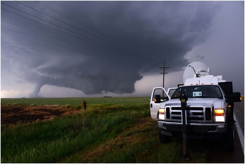
Although research, mobile radars have archived much less data than fixed-site surveillance radars, they still may be used for climate studies that target the characteristics and spatial and temporal distributions of specific small-scale phenomena such as tornadoes and their intensities, sizes, and wind distributions; these phenomena may be probed by fixed-site radars only when they come on rare occasions within 10–20 km of the radars. Thus, climate-variability studies on the nature of mesoscale and convective-scale features are possible. Some difficulties in doing this will involve accounting for the different spatial and temporal resolutions of the different radars ().

c Surface

Section 3.e covered surface measurements and instrumentation that are made globally, so we will mention here some additional networks and measurements usually made on the regional and local scales. Local and state, private and public observing networks have existed for a long time and are still proliferating. The NAS “Network of Networks” report summarized this state of affairs as of 2009, noting that surface networks are viral but not coordinated (NRC, Citation2009). As a result, the National Mesonet Program (NMP) was created by NOAA (https://nationalmesonet.us), and now has more than 40 partners providing data from over 35,000 stations that significantly enhance the Federal networks. Many of these partners are state climate offices (e.g., McPherson et al. (Citation2007)), but also include academic institutions and private sector companies. The majority of observations come from the surface, but a few networks include ground-based profiling systems (e.g. New York State Mesonet; Brotzge et al. (Citation2020)). Other lower-tropospheric measurements come from 450 regional aircraft with TAMDAR sensors. All NMP data are delivered to NCEP’s Meteorological Assimilation Data Ingest System (MADIS), where they are quality controlled and made available for numerical weather prediction and general use.

There are other networks that are not part of the NMP. For example, other agencies such as EPA have stations monitoring air quality, power generation companies have local networks to monitor dispersion of possible pollutants, and the wind power sector uses sodars and lidars to monitor the wind load on their turbines. Ground-based global and regional RF (from VLF to VHF) lightning detection networks (e.g. Earth Networks Total Lightning Network, Vaisala National Lightning Detection Network and Global Lightning Dataset360, World Wide Lightning Location Network, EUCLID, LINET, ATDNet) are operated primarily by private sector companies, though there are regional VHF Lightning Mapping Arrays (LMAs) in the US operated by government laboratories and universities whose data are used operationally by the National Weather Service. The data contain information on lightning location, timing, polarity, in-cloud vs cloud-to-ground, and other parameters (Nag et al., Citation2015). Measurements of electric fields in the vicinity of thunderstorms are made from the ground and balloons. Some surface networks such as Understory (https://understoryweather.com/technology) concentrate on hail detection, with the insurance industry being their primary customer. A list of many U.S. hydrometeorological networks that existed in 2009 is given in Appendix B of NRC (Citation2009), which is based primarily on information from https://archive.eol.ucar.edu/projects/hydrometnet/, which is no longer updated.

A potentially new source of very high-density information about atmospheric conditions comes from the mobile phone industry. Many cell phones have a pressure sensor, which can provide surface pressure information if the height of the phone can be determined (Madaus & Mass, Citation2017). Another opportunistic use of mobile phone networks is to use attenuation by rain of transmissions to and from commercial microwave link towers to estimate hourly and seasonal rainfall distributions in Germany (Graf et al., Citation2020).

d Ground-based and in-situ Profiling Systems

While satellites and radars provide high spatiotemporal resolution measurements both globally and locally, there are still gaps in their coverage. Cloud cover hinders visible and infrared satellite observations, and satellite soundings do not have sufficient vertical resolution to identify fine-scale (10–100 m) structure in the boundary layer. Radars suffer spatial gaps directly above the antenna (cone of silence) and between radars, under the lowest beam. Radars and satellites also do not directly measure common meteorological variables, making retrievals (or forward models in data assimilation) necessary. As a result, many other systems have been developed to fill in these gaps. This subject is more completely discussed in the NAS “Network of Networks” report (NRC, Citation2009), highlighting the importance of surface and boundary layer observations, and a subsequent NAS report summarized boundary layer observations needed for future progress (NRC, Citation2018). Detailed measurement techniques for boundary layer flows are discussed in Kaimal and Finnigan (Citation1994), and a vision for a global boundary layer observing system can be found in Teixeira et al. (Citation2021).

1 In-situ observations

Some instrument systems make measurements as they travel though the atmosphere, such as the radiosondes and dropsondes discussed in Section 3.a.2. These systems are also used to ascertain mesoscale structure during field experiments over land and ocean. Other small and large balloon ascents are made for specialized quantities such as chemical composition, electric fields, etc. Tethered balloon systems, with instruments mounted at regular intervals, are used to sample the planetary boundary layer (PBL). The most rapidly growing in-situ system used to study fine-scale structure are unmanned aerial systems (UAS), sometimes called drones. They can be quite large – e.g. the Global Hawk, which can hover over hurricanes, has a 40 m wingspan – or small, less than 10 cm in diameter. While the Global Hawk can surveil a hurricane at 20 km for over a day, dropping up to 90 dropsondes, NOAA also uses small (1.5 m wingspan), expendable Raytheon Coyote drones, tube-launched from hurricane surveillance aircraft, to sample the lowest layers of tropical storms. UAS are often human-piloted from the ground, but autonomous systems are being developed with pre-planned or adaptive routes. In general, the larger systems are fixed-wing aircraft, while smaller helicopter-type systems are common for more local studies. There are hundreds of applications for UAS systems – one particularly relevant to mesoscale studies is the “3D-Mesonet” concept (Chilson et al., Citation2019) in which a dense array of small UAS (coptersondes – see ) located at surface mesonet stations take lower-tropospheric soundings at regular intervals to assess the rapidly changing boundary layer.

Fig. 10 CopterSonde UAS for atmospheric measurements made by the Center for Automated Sensing Systems at the University of Oklahoma. Photo courtesy of Tony Segalés.

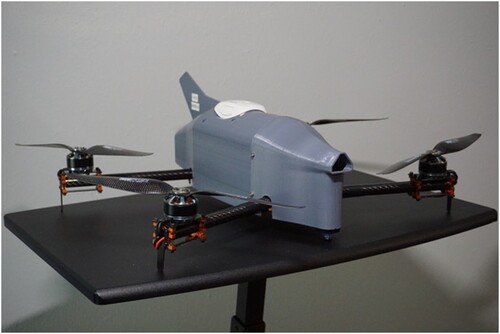
An assessment of the performance of these systems compared to other PBL sensors is presented in Bell et al. (Citation2020). More weather forecasting applications of UAS are discussed in McFarquhar et al. (Citation2020). One PBL sensing opportunity for the future is to instrument the thousands of drones envisioned to deliver packages for Amazon, UPS, etc.; – a benefit to such companies would be improved PBL forecasts. Drones could also be used to transport arrays of microsensors aloft, where they would be released to disperse across a region (Horton et al., Citation2018). Markowski et al. (Citation2018) have described an innovative use of balloon-borne probes that drift along, to a good approximation, with the wind, for making thermodynamic measurements inside convective storms. We note that many of the systems mentioned in this paragraph and elsewhere are examples of “adaptive observations”, in which observing systems are deployed at times and locations where observations are most needed. Field experiments designed to address specific scientific questions are adaptive observation efforts, but the term often refers to real-time strategies to obtain additional, presumably helpful, observations to improve operational forecasts, such as “hurricane hunter” aircraft missions, high-resolution sector scans from satellites, and other deployable systems (see Morss et al., Citation2001).

2 Remote sensing

There are also ground-based remote-sensing systems, both active and passive, that measure tropospheric wind and thermodynamic profiles, although some are limited to within the boundary layer. As previously noted, the NRC (Citation2009) and (Citation2018) reports recommended that networks of profiling systems be installed to provide high resolution (especially in time and in the vertical) measurements of the lower troposphere to complement the high horizontal resolution data we are receiving from satellites, radar and surface stations. Such a Federal network has not yet been installed in the U.S., although many individual systems or small networks have been installed by government agencies, academic institutions or the private sector. Europe has a larger suite of organized PBL sensors (e.g. Illingworth et al., Citation2019). There are several candidate systems that can comprise a ground-based remote-sensing network, some of which (aside from surveillance radars) are described below.

Wind profilers, whose operating principles were discussed in Section 2.b.2.ii, and which are essentially vertically-pointing phased-array Doppler radars, can sense to very high altitudes using VHF frequencies, but, as noted earlier, these do not resolve the boundary layer. Smaller, less-expensive systems, using UHF frequencies, have been designed for lower-tropospheric wind sensing, although the first useful measurement is still 100–200 m above the instrument. For example, a 915 MHz wind profiler can sample at 60 m vertical resolution (with first value at 100 m) up to 4 km, and produce a profile every minute, although more reliable profiles result when averaged over 15–60 min. Wind profiling radars also provide, along with mean Doppler shift, returned power and Doppler spectral width, from which other useful quantities can be determined.

Wind profiler systems are often combined with a radio acoustic sounding system (RASS) which generates vertically-propagating acoustic waves that produce perturbations in the refractive index that are detected by the wind profiler radar if the Bragg scattering condition is met. Since these perturbations are moving at the speed of sound C_s, virtual temperature T_v can be computed from C_s = (γRT_v)^1/2, where R is the gas constant and γ is the ratio of the specific heat capacities at constant pressure and volume, respectively. For UHF boundary layer profilers, temperatures are obtained only up to 1 km or so.

Doppler wind lidars (see 2.c.2) are also candidates for PBL networks, especially if very high-resolution measurements are desired. However, their beams attenuate fairly quickly, limiting their range to several kilometers. Thus, in addition to being frequently used in research field experiments from fixed and mobile platforms (including aircraft), they, along with sodars (2.c.2), are very useful in monitoring wind and turbulence levels at turbine heights in wind energy farms.

Candidates for PBL temperature and moisture measurements include microwave radiometers (MWR), atmospheric emitted radiance interferometers (AERI), and DIAL (see 2.c.1). Upward-looking MWRs can measure temperature, water vapour, and cloud liquid water given careful calibration and ground truth information. Their time resolution is excellent (5 min), but have low vertical resolution – roughly 100’s of m below 1 km, but 1 km or more above 1 km. AERI systems are also passive, examining downwelling radiance in the infrared spectrum to obtain profiles of temperature, water vapour, other gases and aerosols. AERI systems require little maintenance, have 100–200 m vertical resolution and can produce soundings as frequently as 1 min, although intervals of 8–10 min are more common. Comparison of the value of AERI soundings vs other profiling systems described here in cloud-scale NWP can be found in Degelia et al. (Citation2019). DIAL systems for measuring water vapour have shown progress in recent field experiments (Spuler et al., Citation2015). Integrated precipitable water (IPW) can be obtained from the wet delay in overhead GPS transmissions. Many sites providing GPS IPW were installed for geodetic purposes before it was realized that they could also provide accurate hourly IPW data. Slant path water vapour values from GPS transmissions could, in principle, provide 3-D moisture fields via inversion techniques if the paths had sufficiently high spatiotemporal resolution. An excellent summary of lower-troposphere thermodynamic profiling is found in Wulfmeyer et al. (Citation2015).

e Aircraft

1 Radar

Tail-mounted, airborne, X-band radars (e.g. Dowell et al., Citation1997; Hildebrand et al., Citation1996; Marks & Houze, Citation1984; Wakimoto et al., Citation1996) have collected targeted data in severe convective storms and in tropical cyclones and mesoscale convective systems, particularly over the ocean areas. In the U. S. airborne radars are maintained by NOAA, NASA, and NCAR. Airborne radars are particularly useful over otherwise data-sparse regions of the globe. They have been used also over land areas when it is needed to transport radars large distances quickly to get to the target storm. In this regard, they are more responsive than ground-based, mobile radars, but they are also not able to collect data well near the ground, owing to ground-clutter contamination. In addition, since it takes a relatively long time to fly back and forth across a convective storm, the update time of data collection is longer than 5–10 min, during which storms can evolve substantially.

New airborne radars being developed include a phased array, rapid scanning, C-band radar at NCAR, called APAR (Airborne Phased-Array Radar) (https://www.eol.ucar.edu/system/files/APAR%20Brochure%202020-compressed.pdf). This radar should prove valuable for probing weather systems in remote areas very quickly.

2 Other aircraft instrumentation

In addition to the standard parameters provided by commercial aircraft mentioned in III.A.2 and III.B.3, research aircraft can provide these and many more specialized observations. For example, long-range research aircraft can sample variables important for studying radiative forcing and climate change such as atmospheric gas concentrations, aerosols, and upwelling and downwelling solar and terrestrial radiation. Smaller aircraft can be used to probe mesoscale and cloud-scale systems, measuring properties such as liquid water, cloud droplets and other hydrometeors. In addition to the radars described above, research aircraft also deploy lidars and millimetre (cloud) radars.

Several government agencies such as NCAR (for NSF), NASA and NOAA maintain a fleet of aircraft platforms and instruments available to researchers to obtain the atmospheric measurements mentioned above. NCAR operates a long-range Gulfstream V and a C-130; see https://www.eol.ucar.edu/airborne-instrumentation for the possible instrumentation that can be deployed. NOAA’s fleet includes two Lockheed WP-3D Orion “hurricane hunter” aircraft and a Gulfstream IV-SP, that together conduct tropical cyclone surveillance missions (https://www.omao.noaa.gov/learn/aircraft-operations). These planes can be instrumented with a tail Doppler radar for mapping the tropical cyclone wind field as well as a Stepped-Frequency Microwave Radiometer (SFMR) to estimate surface winds. At NASA, the Airborne Science Program (https://airbornescience.nasa.gov/) aircraft are used for calibration and validation of future satellite instrumentation and their retrieval algorithms (Bartlett et al., Citation2018), as well as to collect high temporal and spatial measurements for process studies to complement satellite observations (; ). A detailed description of NASA aircraft scientific missions and accompanying instrumentation is given in a recent NRC report (NRC, Citation2021) that articulates the benefits of airborne platforms to advance earth system science.

Fig. 11 NASA ER-2 instrumentation complement used in the GOES-16 post-launch test field campaign to validate the performance of the GOES-16 ABI and GLM (Padula et al., Citation2016). The VIRIS-NG is the Next-Generation Airborne Visible/Infrared Imaging Spectrometer, LIP is the Lightning Instrument Package (electric field-mills), EXRAD is the ER-2 x-band Doppler radar, CPL is the Cloud Physics Lidar, GCAS is the GeoCAPE Airborne Simulator, S-HIS is the High-resolution Interferometer Sounder, CRS is the 94 GHz (W-band) Cloud Radar System, and FEGS is the Fly’s Eye GLM Simulator. Refer to (https://airbornescience.nasa.gov/) for additional instrument details.

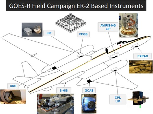
Table 4. NASA ER2 instrument complement used in the GOES-16 post-launch test campaign. The instrument specs include type of measurement, spectral range, spectral resolution, ground sample distance (GSD), field of view (FOV), and swath width.

Download CSV Display Table

A few universities operate small research aircraft, primarily for cloud physics research; e.g. the University of Wyoming King Air (http://www.atmos.uwyo.edu/uwka/users/capabilities.shtml), and the University of North Dakota Citation (http://airborneresearch.atmos.und.edu). Researchers can often add their own instrumentation to any of the above aircraft provided weight, size and power limitations are met.

f Ships

Ships have been making weather observations for centuries, which enabled Edmund Halley, e.g. to propose a mechanism for the monsoon as early as the late seventeenth century (Halley, Citation1686). The WMO specifications for ship observations include current weather, temperature, dewpoint temperature, pressure, pressure tendency, wind speed and direction, visibility, cloud amount, type and heights, seawater temperature, sea wave state, sea ice, and icing on ship, along with the course, speed and location of the ship. Ship observations are not as reliable as those on land, owing to, e.g. the ship’s motion, non-standard siting, height about sea level, and reliance on human observations. Fortunately, the sea surface temperature, an important variable for both weather forecasting and climate, can be done automatically through ship water intakes and satellites. Ships are frequently used in field experiments, and thus can support many other observation systems such as radiosondes, and remote sensing systems. Buoys, both fixed and drifting, also measure standard meteorological parameters, sea surface temperature, salinity and wave heights (see, e.g. https://www.ndbc.noaa.gov). It is beyond the scope of this paper to cover all oceanographic measurements, but one promising new system is Saildrone (https://www.saildrone.com), a small, uncrewed, wind and solar-powered vessel that can roam the open ocean and measure many physical quantities above and below the surface (Meinig et al., Citation2019). Radars have been placed on ships during field experiments in remote oceanic areas, particularly in the tropics. The attitude of the ship in the water must be carefully measured and accounted for before the data can be used. Data from these radars during specific field experiments (too numerous to list here) may be available online. A rich source of data is available from NCAR at the EOL (Earth Observing Laboratory) (https://www.eol.ucar.edu/data-software/field-catalog), where data from other observing systems on other platforms may also be found.

Finally, we will note here that oceanic surface wind measurements from ships, buoys, and drones can be supplemented immensely by scatterometer instruments hosted on satellites, which uses radar to measure backscatter from the ocean surface to determine wind speed and direction. An Advanced Scatterometer (ASCAT) is currently aboard the EUMETSAT Metop satellites, and its wind products are extremely useful to those monitoring oceanic storms, especially hurricanes (see https://www.eumetsat.int/ascat).

5 Some observation issues

a Coordination among Observing System Providers

While meteorological observing system infrastructure has historically been provided by national governments, a large amount of data is now being provided by the private sector, academia and smaller public institutions (states, cities, etc.). Examples range from GPS-RO CubeSats to mobile and fixed radar and wind-profiler networks, to state and city mesonets, down to citizen surface weather observations. As outlined in NRC (Citation2009), there are many organizational models for such networks, from public systems publicly available (e.g. NEXRAD), to private systems with private data (NLDN), public systems with private data (DoD observations), private systems with public data (MDCRS) and various hybrids (e.g. DFW Urban Testbed, Brewster et al., Citation2017). NRC (Citation2009) noted that an impression of “false sparsity” could result if observations from these diverse sources were not identified or used, and presented recommendations for how the various data owners could coordinate to help set standards and make these data widely available.

Owing to the investments involved, the satellite community began such an effort in 1972 with the formation of the Coordination Group for Meteorological Satellites (CGMS), initially to coordinate geostationary meteorological satellites. They have expanded their membership and activities to monitor, intercalibrate, improve, and harmonize the quality of observations from weather and environmental satellites of the Integrated Global Observing System. In 2005, they and the WMO initiated the Global Space-based Inter-Calibration System (GSICS), an international collaborative effort comprised of operational and research space agencies, to ensure consistent accuracy among space-based observations worldwide for climate monitoring, weather forecasting, and environmental applications (https://gsics.wmo.int).

Similar efforts exist, both internationally and nationally, to coordinate and intercompare other observing systems such as radars, radiosondes, ground-based remote sensing, soil moisture, rainfall, snow depth/ SWE, and surface networks, some of which have been mentioned in the text. For surface networks, recommendations for siting standards and metadata exist (Fiebrich et al., Citation2020), although they are not always followed. The major NWP centres of the world have become de facto data evaluation hubs owing to their sophisticated quality control procedures and FSOI results (see Section 5.b.3). Thus, they can inform data owners if, e.g. a systematic error or bias appears in their observing system or at an individual station, or if their entire system is not adding any value to the forecasts. Through these checks, it is hoped that errors can be corrected and that nations/companies can eliminate redundant systems and invest where the greatest observational needs exist.

b Data Assimilation Considerations

1 Synergy among observations, data assimilation and models

There is great synergy among observations, data assimilation (DA) systems and numerical forecast models in that improvements to any one component causes improvements to the others, or, conversely, deficiencies in one negatively affects the others. We should note that in the feedback to observations case, improvements to DA-NWP systems don’t “improve” observations but, as mentioned in Section 5.a, they provide better feedback on the errors and value of the observations, which should motivate improving observation accuracy and development of new or enhanced observing systems. DA systems, though, have the responsibility of making optimal use of the data that they do receive, a challenging task given the hundreds of sensors on dozens of satellites, not to mention the many additional inputs from in situ and ground-based systems. There is the well-known example of the large increase in forecast model skill when DA systems began to use satellite radiances directly (which is a very accurate measurement) rather than the retrieved temperature profiles, which had significant errors. The responsibility of models is to represent the physics as faithfully as possible, as no amount of accurate high-resolution observations or sophistication in a DA system can overcome, e.g. a model’s poor representation of PBL physics, which will create its own incorrect structure once the DA cycle is complete. In some situations, such as modelling the land surface properties during a forecast, there are insufficient observations to accurately characterize all the components of the surface energy balance, such as soil moisture profiles, in the initial state. Thus, land data assimilation systems (LDAS) were developed to assimilate observed fields such as precipitation and satellite imagery with the model physics to attain all the necessary fields. More generally, DA accomplishes “information spreading” into areas with fewer observations, which might appear to decrease the need for new observations, but if those areas have unobserved mesoscale structures or topography, then the need for higher resolution observations returns.

2 Example of current challenge: all-sky radiances

A current example of a challenging problem in making optimal use of existing data is the assimilation of all-sky radiances. Such radiances come from microwave sounders (e.g. AMSU-A for temperature, AMSU-B for moisture), IR sounders (e.g. CrIS, IASI) and multispectral imager IR channels. Until recently, model cloud fields were not accurate enough to provide a good match to observed radiances in the forward model step (when model fields are converted to radiances and brought to observation locations), and thus all satellite views that contained clouds were not used in DA. However, increased resolution and improved physics are resulting in better cloud fields, which permits attempting to correct model cloud-contaminated radiances with radiances that come from satellite views that contain clouds. This was first successful for microwave radiances which are less affected by clouds (Geer et al., Citation2014) but only more recently with IR radiances, which are very cloud sensitive. Geer et al. (Citation2019) and Chan et al. (Citation2020) discuss the challenges involved in the use of all-sky IR radiances in global and storm-scale models, respectively. For the global case, Geer et al. (Citation2019) found that all-sky IR DA adds 65% more observations than clear-sky-only assimilation, and had a significant positive impact on forecasts, especially in the tropics.

3 Assessment of observations

Data assimilation (DA) and modelling systems can be used to assess the benefit (or lack thereof) of individual and combined observing systems. Observing System Experiments (OSE) (often called data denial experiments) are employed to evaluate current observations. Forecasts made using all available data are compared with ones made with one or more observing systems absent, thus assessing the impact of the denied data. An example of a regional OSE study of several of the ground-based observing systems mentioned in this paper is given by James and Benjamin (Citation2017), and an OSE for the global scale is presented by Bouttier and Kelly (Citation2001). Note that OSEs can also be used to see how effectively the DA system uses a particular set of observations. To assess the potential value of future observing systems, Observing System Simulation Experiments (OSSE) are used. Here, both current and future observations (and their errors) have to be simulated from a “nature run”, which is usually a very high-resolution forecast (made by a different model than used in the experiments) designed to simulate the atmosphere as accurately as possible. Data denial experiments are then conducted to assess the impact of the future observations. OSSEs can also be used help design new observing networks and their sampling strategies, as well to assess whether a new observing capability can help improve our characterization of the earth system or our understanding of the processes that govern the system. A recent essay on current and past applications of OSSEs and recommendations for their future use is given by Zeng et al. (Citation2020), while Hoffman and Atlas (Citation2016) provide more detail on the OSSE methodology.

Real-time, simultaneous evaluation of the forecast impact of individual observations and observing systems are made by operational modelling centres using the Forecast Sensitivity to Observations (FSO) technique. This method, often called Forecast Sensitivity to Observations Impact (FSOI), uses the linear tangent model of an adjoint- variational DA system (4DVar) to measure the reduction of a specified forecast error metric resulting from the addition of new observations (Langland & Baker, Citation2004). This technique can also be used for ensemble Kalman filter DA systems as outlined by Kalnay et al. (Citation2012), where it is known as EFSO or EFSOI. Examples using these techniques are given by Gelaro and Zhu (Citation2009), Gelaro et al. (Citation2010), Cardinali (Citation2018), Diniz and Todling (Citation2020), and Kotsuki et al. (Citation2019); note that all these authors caution against over-interpretation of the results owing to the various approximations and limitations of the techniques. An example of the output of a FSOI system is given in , which shows how FSOI results change over time in the Goddard Modeling and Assimilation Office (GMAO) global model, with the left figure showing changes from 2012–13 to 2018–19, and the right figure with changes from 2017–18 to 2019–20.

Fig. 12 Forecast Sensitivity to Observations Impact (FSOI) ranking comparison (courtesy of Will McCarty, NASA Goddard Modeling and Data Assimilation Office (GMAO)).

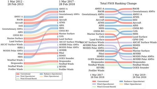
As is common in many global FSOI experiments, microwave (AMSU-A) and hyperspectral (IASI) sounders rank high (see also figures in the Cotton & Eyre, Citation2019; study referenced in Section 3.a.2). Here, radiosonde observations and atmospheric motion vectors (AMV) also rank high in positive impact. A very recent result from GMAO ( – from https://gmao.gsfc.nasa.gov/forecasts/systems/fp/obs_impact/ – McCarty, personal communication) shows observation impacts computed using the adjoint of the GEOS-5 atmospheric data assimilation system run at GMAO.

Fig. 13 Observation impacts computed using the adjoint of the Goddard Earth Observing System, Version 5 (GEOS-5) atmospheric data assimilation system at NASA GSFC. The average values for each observing system are shown over the full year 19 March 2020–18 March 2021. The values are averaged over the number of cases in the interval, and the colour shading denotes the average number of observations for a given observing system. Observation impacts in GEOS-5 are computed once each day for the 24-h forecast initialized at 00Z. The results shown are from the GEOS-5 interactive web page (https://gmao.gsfc.nasa.gov/forecasts/systems/fp/obs_impact/).

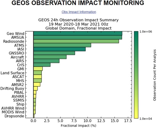
As in , observation impact is taken to be the difference in the error measure between 24-h forecasts initialized from the final analysis and corresponding background state, where this difference is due entirely to the assimilation of the observations. Positive values of observation impact indicate that assimilation of a given set of observations has improved the 24-h forecast. These results show that GEO-AMV winds now have the largest impact. This may be attributable to the increase of continuous AMV observations from GEO that cover much of the full disk of the earth. Note that the data count (see colour scale) for AMVs is as large as for the IASI and AMSU-A systems, which may not be true for other global modelling systems, depending on the quality control and data selection procedures used on the raw satellite data, which is on the order of 10⁸ observations.

c Data Curation

1 NASA's Earth Observing System Data and Information System (EOSDIS)

NASA's Earth Observing System Data and Information System (EOSDIS) is designed as a distributed system, with major facilities at NASA's Distributed Active Archive Centers (DAACs) located throughout the United States. These institutions are custodians of NASA’s Earth Observing System (EOS) mission data and ensure that data will be easily accessible to users. EOSDIS DAACs process, archive, document, and distribute data from NASA's past and current satellites (https://earthdata.nasa.gov/eosdis/science-system-description/eosdis-services).

2 NOAA’s Comprehensive Large Array-data Stewardship System (CLASS)

The Comprehensive Large Array-data Stewardship System (CLASS) managed by the NOAA National Centers for Environmental Information (NCEI) is an electronic library of NOAA environmental data. CLASS provides data through a terrestrial connection and is NOAA’s web-based data archive and distribution system for NOAA environmental data (satellite, radar, surface, in-situ, other). CLASS provides data access and distribution services of NOAA and US DoD Polar Operational Environmental Satellites (POES) data, NOAA’s GOES data, and derived data. CLASS has a rolling window of data available, subscriptions, and bulk orders for larger user needs. CLASS stores an average of 130 TB/month of data. The CLASS registration process is available at https://www.class.noaa.gov/notification/demo.htm.

3 ESA/EUMETSAT Data centers

The European Space Agency (ESA) distributes Earth Observation (EO) data from ESA Missions, Third Party Missions (TPMs), ESA Campaigns, the Copernicus Space Component (CSC), and auxiliary data from a number of missions and instruments (https://earth.esa.int/web/guest/data-access/how-to-access-esa-data). ESA also has a collection of airborne, ground-based, or balloon campaigns over different locations inside and outside Europe. The resulting datasets are available on the internet or media. Data distributed by ESA is available under different data policies and access mechanisms.

The EUMETSAT Data Center (https://www.eumetsat.int/eumetsat-data-centre). has more than 300 meteorological satellite products available – in the case of Meteosat spanning a record of more than 30 years (since 1981). The Data Centre offers one of Europe’s largest and most comprehensive collections in this field. EUMETSAT Data Center products, once they are ready to be delivered, can be accessed online or physically sent to the user on the chosen media. The Atmospheric Toolbox (https://earth.esa.int/eogateway/tools/atmospheric-toolbox) provides scientists with tools for ingesting, processing, and analyzing atmospheric remote sensing data.

4 UCAR Research Data Archive (RDA)

The Research Data Archive (RDA) (https://rda.ucar.edu/) is maintained by the Computational and Information Systems Laboratory (CISL) at the National Center for Atmospheric Research, which is managed by UCAR and sponsored by the National Science Foundation. The archive contains a diverse collection of meteorological and oceanographic observations, operational and reanalysis model outputs, and remote sensing datasets to support atmospheric and geosciences research. The NCAR Earth Observing Laboratory also manages a widely used Field Catalog service (http://catalog.eol.ucar.edu) offering a comprehensive collection of field project related documents and data sets. Each Field Catalog is customized as needed for each campaign and continues to be available on-line long after the field campaign has ended, so data can be used for post-project analysis.

5 Cloud Service Providers

NASA and NOAA and other data centres are actively moving data to the cloud. For example, the Global Hydrology Resource Center (GHRC) was the first of the 12 NASA Distributed Active Archive Centers (DAACs) to migrate all its data holdings to a commercial cloud provider (Amazon Web Services) mapping out a pathway for the other DAACs (https://earthdata.nasa.gov/learn/articles/tools-and-technology-articles/eosdis-cumulus-project). The GHRC manages data from satellites, aircraft campaigns, in-situ sensors, and computer models. Previously, it might have taken weeks to download, reformat, and restructure the data needed to do a time-series analysis, a task that will eventually be completed in minutes. New tools for data exploitation can eliminate the need to download large volumes of data to a local data repository or computer for research analysis. The general public can access data and tools made available through the Cloud Service Providers (CSPs) for free, and the data are available to the public without restriction on use. These data will include the original and unaltered data content, and may additionally be provided using any broadly accessible and open format or formats. NOAA’s Big Data Program (https://www.noaa.gov/organization/information-technology/big-data-program) works with three infrastructure-as-a-service (IaaS) providers to broaden access to NOAA’s data resources. These partnerships are designed to not only facilitate full and open data access at no net cost to the taxpayer, but also foster innovation by bringing together the tools necessary to make NOAA's data more readily accessible. See also https://earthdata.nasa.gov/eosdis/cloud-evolution.

d Final Remarks

All branches of science require observations to inform their discipline and atmospheric science is no exception. As has documented in this paper, the atmosphere is very well monitored, with terabytes of information per day being generated from satellites, radars and hundreds of other observing systems and instruments. This does not mean that the atmosphere is perfectly observed or that we are making optimal use of the data that we do have. Every advance in numerical weather prediction and climate simulations caused by new observations, better data assimilation, higher resolution and improved physics motivates a desire to increase our capabilities in all four areas. For example, research has shown that climate models with convection-allowing resolution have superior results over coarser models – to accomplish this we’ll need additional observations to provide more detailed characterization of the earth’s surface and atmospheric composition, observations to inform improved model physics, and, since climate models are becoming well-coupled with ocean, sea ice, land-surface, air chemistry and hydrologic models, we’ll need more observations in those domains as well. On the storm scale, the NWS has the “Warn-on-Forecast” vision, in which sub-kilometer resolution models provide reliable probabilities for hazardous weather, including tornadoes, hours before they occur. This will require far more rapid scanning, such as might be provided by a national phased-array radar network (NRC, Citation2002), plus other ground-based systems to fill in radar gaps and provide high-resolution PBL profiling, along with high-resolution satellite data. Both these model advances (coupled global and convection-resolving) will require advanced but efficient DA techniques, enhanced high performance computing capabilities and greater communication and archival demands. To sustain observations made on operational networks, especially on the synoptic scale, we must rapidly adjust to circumstances that force long-term observing stations to cease operations, whether from changing environmental conditions such as beach erosion, natural disasters such as fires or severe storms, or from lack of continuing funding.

There is no shortage of studies that provide vision and specific recommendations for future observational needs. For example, the NRC (Citation2009) “Network of Networks” report’s recommendations articulated the need for a national network of ground-based profiling systems to provide enhanced observations in the PBL, whose need has been reinforced by several subsequent NAS studies, including the recent NRC PBL Workshop (Citation2018) report. For satellites, the U.S. is guided by the NASA-funded NAS decadal studies, the most recent being Thriving on Our Changing Planet (NRC, Citation2018), which presents prioritized science, applications, and observations, with related strategic and programmatic guidance, to support the U. S. civil space Earth observation programme over the coming decade. Also, the World Meteorological Organization (WMO) published Vision for the WMO Integrated Global Observing System (WIGOS) Vision for 2040, which presents a likely scenario of how user requirements for observational data may evolve over the next 20 years (WMO, Citation2019). Motivated by these and other studies, NOAA, NASA and other international atmospheric science and space agencies have teams working on components of the future satellite constellation, which will feature advanced instruments with higher spectral and spatial resolution in both LEO and GEO orbits. These agencies as well as the private sector are also developing and launching swarms of Cubesats that may revolutionize the future of satellite architectures and how data are distributed and shared. We will see an explosive growth in new approaches that combine the radiances and retrieved information from passive and active sensors from multiple platforms, and increasingly employ Artificial Intelligence/Machine Learning (AI/ML) techniques, data analytics, visualization, and cloud data and software for an integrated depiction of the atmosphere and the Earth as a System.

Disclosure statement

No potential conflict of interest was reported by the author(s).

Additional information

Funding

H. Bluestein is supported by NSF grant AGS 1947146. F. Carr acknowledges support from the National Weather Service's National Mesonet Program over the past few years. S. Goodman was supported in part by NASA Grant 80NSSC18K1689.

Notes

1 Electronically scanning radars are typically phased-array radars that are steered through hardware phase shifters, by changing the frequency slightly, or via software.

2 Each beam may be from a separate antenna or from a phased-array antenna (Balsley & Gage, Citation1982).

3 Since we do not include atmospheric chemistry in this review, we will not go into the details of pollutant measurement.

4 The BWER was first referred to as a “vault.”

References

Aberson, S., & Franklin, J. (1999). Impact on hurricane track and intensity forecasts of GPS dropwindsonde observations from the first-season flights of the NOAA gulfstream-IV Jet aircraft. Bulletin of the American Meteorological Society, 80(3), 421–427. https://doi.org/10.1175/1520-0477(1999)080<0421:IOHTAI>2.0.CO;2
Web of Science ®Google Scholar
Ackerman, S. A., Platnick, S., Bhartia, P. K., Duncan, B., L’Ecuyer, T., Heidinger, A., Skofronick-Jackson, G., Loeb, N., Schmit, T., & Smith, N. (2019). Satellites see the world’s atmosphere. Meteorological Monographs, 59, 4.1–4.53. https://doi.org/10.1175/AMSMONOGRAPHS-D-18-0009.1
Google Scholar
Adirosi, E., Baldini, L., & Tokay, A. (2020). Rainfall and DSD parameters comparison between Micro Rain Radar, two-dimensional video and Parsivel disdrometers, and S-band dual-polarization radar. Journal of Atmospheric and Oceanic Technology, 37(4), 621–640. https://doi.org/10.1175/JTECH-D-19-0085.1
Web of Science ®Google Scholar
Anagoustou, E. N., & Krajewski, W. F. (1999). Real-time radar rainfall estimation. Part I: Algorithm formulation. Journal of Atmospheric and Oceanic Technology, 16(2), 189–197. https://doi.org/10.1175/1520-0426(1999)016<0189:RTRREP>2.0.CO;2
Web of Science ®Google Scholar
Apke, J. M., Hilburn, K. A., Miller, S. D., & Peterson, D. A. (2020). Towards objective identification and tracking of convective outflow boundaries in next-generation geostationary satellite imagery. Atmospheric Measurement Techniques, 13(3), 1593–1608. https://doi.org/10.5194/amt-13-1593-2020
Web of Science ®Google Scholar
Apke, J. M., Mecikalski, J. R., & Jewett, C. P. (2016). Analysis of mesoscale atmospheric flows above mature deep convection using super rapid scan geostationary satellite data. Journal of Applied Meteorology and Climatology, 55(9), 1859–1887. https://doi.org/10.1175/JAMC-D-15-0253.1
Web of Science ®Google Scholar
Armijo, L. (1969). A theory for the determination of wind and precipitation velocities with Doppler radars. Journal of the Atmospheric Sciences, 26(3), 570–573. https://doi.org/10.1175/1520-0469(1969)026<0570:ATFTDO>2.0.CO;2
Web of Science ®Google Scholar
Austin, P. M. (1987). Relation between measured radar reflectivity and surface rainfall. Monthly Weather Review, 115(5), 1053–1070. https://doi.org/10.1175/1520-0493(1987)115<1053:RBMRRA>2.0.CO;2
Web of Science ®Google Scholar
Ayasse, A. K., Dennison, P. E., Foote, M., Thorpe, A. K., Joshi, S., Green, R. O., Duren, R. M., Thompson, D. R., & Roberts, D. A. (2019). Methane mapping with future satellite imaging spectrometers. Remote Sensing, 11(24), 3054. https://doi.org/10.3390/rs11243054
Web of Science ®Google Scholar
Balsley, B. B., & Gage, K. (1982). On the use of radars for operational wind profiling. Bulletin of the American Meteorological Society, 63(9), 1009–1018. https://doi.org/10.1175/1520-0477(1982)063<1009:OTUORF>2.0.CO;2
Web of Science ®Google Scholar
Banta, R. M. (1995). Sea breezes shallow and deep on the California coast. Monthly Weather Review, 123(12), 3614–3622. https://doi.org/10.1175/1520-0493(1995)123<3614:SBSADO>2.0.CO;2
Web of Science ®Google Scholar
Bartlett, B., Casey, J., Padula, F., Pearlman, A., Pogorzala, D., & Cao, C. (2018). Independent validation of the advanced baseline imager (ABI) on NOAA's GOES-16: Post-launch ABI airborne science field campaign results. Proceedings of the Society of Photo-optical Instrument Engineers, SPIE 10764, Earth Observing Systems XXIII, 107640H, 19-23 August, 2018. https://doi.org/10.1117/12.2323672
Google Scholar
Bauwens, M., Compernolle, S., Stavrakou, T., Müller, J.-F., Gent, J., Eskes, H., Levelt, P. F., Van der A, R., Veefkind, J. P., Vlietinck, J., Yu, H., & Zehner, C. (2020). Impact of coronavirus outbreak on NO2 Pollution assessed using TROPOMI and OMI observations. Geophysical Research Letters, 47(11), https://doi.org/10.1029/2020GL087978
PubMed Web of Science ®Google Scholar
Bedka, K. M., Murillo, E., Homeyer, C. R., Scarino, B., & Mersiovski, H. (2018). The above anvil cirrus plume: An important severe weather indicator in visible and infrared satellite imagery. Journal of Applied Meteorology, 33, 1159–1181. https://doi.org/10.1175/WAF-D-18-0040.1
Google Scholar
Bell, T. M., Greene, B. R., Klein, P. M., Carney, M., & Chilson, P. B. (2020). Confronting the boundary layer data gap: Evaluating new and existing methodologies of probing the lower atmosphere. Atmospheric Measurement Techniques, 13(7), 3855–3872. https://doi.org/10.5194/amt-13-3855-2020
Web of Science ®Google Scholar
Bilbro, J. W., Fichtl, G., Fitzjarrald, D. E., Krause, M., & Lee, R. W. (1984). Airborne Doppler lidar wind field measurements. Bulletin of the American Meteorological Society, 65(4), 348–359. . https://doi.org/10.1175/1520-0477(1984)065<0348:ADLWFM>2.0.CO;2
Web of Science ®Google Scholar
Blakeslee, R. J., Lang, T. J., Koshak, W. J., Buechler, D., Gatlin, P., Mach, D. M., Stano, G. T., Virts, K. S., Walker, T. D., Cecil, D. J., Ellett, W., Goodman, S. J., Harrison, S., Hawkins, D. L., Heumesser, M., Lin, H., Maskey, M., Schultz, C. J., Stewart, M., Bateman, M., Chanrion, O., & Christian, H. (2020). Three years of the lightning imaging sensor onboard the International Space Station: Expanded global coverage and enhanced applications. Journal of Geophysical Research – Atmospheres, Earth and Space Science, 125, e2020JD032918. https://doi.org/10.1029/2020JD032918
Web of Science ®Google Scholar
Bluestein, H., Rauber, R. M., Burgess, D. W., Albrecht, B., Ellis, S. M., Richardson, Y. P., Jorgensen, D. P., Frasier, S. J., Chilson, P., Palmer, R. D., Yuter, S. E., Lee, W.-C., Dowell, D. C., Smith, P. L., Markowski, P. M., Friedrich, K., & Weckwerth, T. M. (2014). Radar in the atmospheric sciences and related research: Current systems, emerging technology, and future needs. Bulletin of the American Meteorological Society, 95(12), 1850–1861. https://doi.org/10.1175/BAMS-D-13-00079.1
Web of Science ®Google Scholar
Bluestein, H. B. (1992). Synoptic-dynamic meteorology in Midlatitudes, Vol. I: Principles of kinematics and dynamics. Oxford University Press.
Google Scholar
Bohren, C. F., & Albrecht, B. A. (1998). Atmospheric thermodynamics. Oxford University Press. https://doi.org/10.1119/1.1313524
Google Scholar
Bouttier, F., & Kelly, G. (2001). Observing-system experiments in the ECMWF 4D-Var data assimilation system. Quarterly Journal of the Royal Meteorological Society, 127(574), 1469–1488. https://doi.org/10.1002/qj.49712757419
Web of Science ®Google Scholar
Brandes, E. A., Zhang, G., & Vivekanandan, J. (2003). An evaluation of a drop distribution-based polarimetric radar rainfall estimator. Journal of Applied Meteorology, 42(5), 652–660. https://doi.org/10.1175/1520-0450(2003)042<0652:AEOADD>2.0.CO;2
Google Scholar
Brewster, K. A., Bajij, A., Phillips, B. J., Pepyne, D. L., Lyons, E., & Carr, F. (2017). CASA Dallas-Fort Worth urban testbed observations: Networks of networks at work [Special Symposium on Meteorological Observations and Instruments]. 97th American Meteorological Society Annual Meeting, 22-26 January, Seattle, WA.
Google Scholar
Brock, F. V., & Richardson, S. J. (2001). Meteorological measurement systems. Oxford University Press. https://doi.org/10.1093/oso/9780195134513.001.0001
Google Scholar
Brotzge, J. A., Wang, J., Thorncroft, C. D., Joseph, E., Bain, N., Bassill, N., Farruggio, N., Freedman, J. M., Hemker, K., Johnston, D., Kane, E., McKim, S., Miller, S. D., Minder, J. R., Naple, P., Perez, S., Schwab, James J., Schwab, M. J., & Sicker, J. (2020). A technical overview of the New York State Mesonet standard network. Journal of Atmospheric and Oceanic Technology, 37(10), 1827–1845. https://doi.org/10.1175/JTECH-D-19-0220.1
Web of Science ®Google Scholar
Brown, R. A., Lemon, L. R., & Burgess, D. W. (1978). Tornado detection by pulsed Doppler radar. Monthly Weather Review, 106(1), 29–38. https://doi.org/10.1175/1520-0493(1978)106<0029:TDBPDR>2.0.CO;2
Web of Science ®Google Scholar
Browning, K. A., & Donaldson, R. J., Jr. (1963). Airflow and structure of a tornadic storm. Journal of the Atmospheric Sciences, 20(6), 533–545. https://doi.org/10.1175/1520-0469(1963)020<0533:AASOAT>2.0.CO;2
Web of Science ®Google Scholar
Bruneau, D., Quaglia, P., Flamant, C., & Pelon, J. (2001). Airborne lidar LEANDRE II for water-vapor profiling in the troposphere II first results. Applied Optics, 40(21), 3462–3475. https://doi.org/10.1364/AO.40.003462
PubMed Web of Science ®Google Scholar
Cardinali, C. (2018). Forecast sensitivity observation impact with an observation-only based objective function. Quarterly Journal of the Royal Meteorological Society, 144(716), 2089–2098. https://doi.org/10.1002/qj.3305
Web of Science ®Google Scholar
Chan, M.-Y., Zhang, F. Q., Chen, X. C., & Leung, L. R. (2020). Potential impacts of assimilating all-sky satellite infrared radiances on convection-permitting analysis and prediction of tropical convection. Monthly Weather Review, 148(8), 3203–3224. https://doi.org/10.1175/MWR-D-19-0343.1
Web of Science ®Google Scholar
Chance, K. V., Liu, X., Suleiman, R. M., Flittner, D. E., Al-Saadi, J., & Janz, S. J. (2013). Tropospheric emissions: Monitoring of pollution (TEMPO). Proceedings Society Photo-Optical Instrumentation Engineers (SPIE) 8866, Earth Observing Systems XVIII, ed. Butler, J. J., Xiong, X., & Gu, X., 88660D. https://doi.org/10.1117/12.2024479
Google Scholar
Chilson, P. B., Bell, T. M., Brewster, K. A., Britto Hupsel de Azevedo, G., Carr, F. H., Carson, K., Doyle, W., Fiebrich, C. A., Greene, B. R., Grimsley, J. L., Kanneganti, S. T., Martin, J., Moore, A., Palmer, R. D., Pillar-Little, E. A., Salazar-Cerreno, J. L., Segales, A. R., Weber, M. E., Yeary, M., & Droegemeier, K. K. (2019). Moving towards a network of autonomous UAS atmospheric profiling stations for observations in the Earth’s lower atmosphere: The 3D Mesonet concept. Sensors, 19(12), 2720. https://doi.org/10.3390/s19122720
PubMed Web of Science ®Google Scholar
Collard, A. D., & McNally, A. P. (2009). Infrared atmospheric sounding interferometer radiances at ECMWF. Quarterly Journal Royal Meteorological Society, 135(641), 1044–1058. https://doi.org/10.1002/qj.410
Web of Science ®Google Scholar
Cotton, J., & Eyre, J. (2019). Forecast sensitivity to observations impact (FSOI) by country or region. Met Office Forecasting Research Technical Report, No. 636.
Google Scholar
Crum, T. D., & Alberty, R. L. (1993). The WSR-88D and the WSR-88D operational support test facility. Bulletin of the American Meteorological Society, 74(9), 1669–1687. https://journals.ametsoc.org/view/journals/bams/74/9/1520-0477_1993_074_1669_twatwo_2_0_co_2.xml https://doi.org/10.1175/1520-0477(1993)074<1669:TWATWO>2.0.CO;2
Web of Science ®Google Scholar
Deepak, A. (1977). Inversion methods in atmospheric remote sensing. Academic Press. https://doi.org/10.1016/B978-0-122-08450-8.X5001-2
Google Scholar
Degelia, S. K., Wang, X., & Stensrud, D. J. (2019). An evaluation of the impact of assimilating AERI retrievals, kinematic profilers, rawinsondes, and surface observations on a forecast of a nocturnal convection initiation event during the PECAN field campaign. Monthly Weather Review, 147(8), 2739–2764. https://doi.org/10.1175/MWR-D-18-0423.1
Web of Science ®Google Scholar
Diniz, F. L. R., & Todling, R. (2020). Assessing the impact of observations in a multi-year reanalysis. Quarterly Journal of the Royal Meteorological Society, 146(727), 724–747. https://doi.org/10.1002/qj.3705
Web of Science ®Google Scholar
Doviak, R. J., Bringi, V., Ryzhkov, A., Zahrai, A., & Zrnić, D. (2000). Considerations for polarimetric upgrades to operational WSR-88D radars. Journal of Atmospheric and Oceanic Technology, 17(3), 257–278. https://doi.org/10.1175/1520-0426(2000)017<0257:CFPUTO>2.0.CO;2
Web of Science ®Google Scholar
Doviak, R. J., & Zrnić, D. S. (2006). Doppler radar and weather observations (2nd ed.). Dover.
Google Scholar
Dowell, D. C., Bluestein, H. B., & Jorgensen, D. P. (1997). Airborne Doppler radar analysis of supercells during COPS-91. Monthly Weather Review, 125(3), 365–383. https://doi.org/10.1175/1520-0493(1997)125<0365:ADRAOS>2.0.CO;2
Web of Science ®Google Scholar
Ecklund, W. L., Carter, D. A., & Balsley, B. B. (1988). A UHF wind profiler for the boundary layer: Brief description and initial results. Journal of Atmospheric and Oceanic Technology, 5(3), 432–441. https://doi.org/10.1175/1520-0426(1988)005<0432:AUWPFT>2.0.CO;2
Google Scholar
Emeis, S. (2010). Measurement methods in atmospheric sciences. Borntraeger Science Publishers. https://doi.org/10.1002/met.250
Google Scholar
Esmaili, R., Smith, N., Berndt, E. B., Dostalek, J. F., Kahn, B. H., White, K., Barnet, C. D., Sjoberg, W., & Goldberg, M. (2020). Adapting satellite soundings for operational forecasting within the hazardous weather testbed. Remote Sensing, 12(5), 886. https://doi.org/10.3390/rs12050886
Web of Science ®Google Scholar
Eyre, J. (1997). Variational assimilation of remotely-sensed observations of the atmosphere. Journal of the Meteorological Society of Japan, 75, 331–338. https://doi.org/10.2151/jmsj1965.75.1B_331
Web of Science ®Google Scholar
Fabry, F. (2015). Radar meteorology: Principles and practice. Cambridge University Press.
Google Scholar
Farrell, S. L., Duncan, K., Buckley, E. M., Richter-Menge, J., & Li, R. (2020). Mapping sea ice surface topography in high fidelity With ICESat-2. Geophysical Research Letters, 47(21), https://doi.org/10.1029/2020GL090708
Web of Science ®Google Scholar
Ferraro, R. R., Weng, F., Grody, N. C., Zhao, L., Meng, H., Kongoli, C., Pellegrino, P., Qiu, S., & Dean, C. (2005). NOAA operational hydrological products derived from the advanced microwave sounding unit. IEEE Transactions on Geoscience and Remote Sensing, 43(5), 1036–1049. https://ieeexplore.ieee.org/document/1424280. https://doi.org/10.1109/TGRS.2004.843249
Web of Science ®Google Scholar
Fiebrich, C. A., Brinson, K. R., Mahmood, R., Foster, S. A., Schargorodski, M., Edwards, N. L., Redmond, C. A., Atkins, J. R., Andresen, J. A., & Lin X. (2020). Toward the standardization of mesoscale meteorological networks. Journal of Atmospheric and Oceanic Technology, 37(11), 2033–2049. https://doi.org/10.1175/JTECH-D-20-0078.1
Web of Science ®Google Scholar
Fletcher, J. O., Swingle, D. M., Katz, I., Harney, P. J., Austin, P. M., Geotis, S. G., Metcalf, J. I., Glover, K. M., Kessler, E., Probert-Jones, J. R., Douglas, R. H., Kodaira, N., Aoyagi, J., Kulshrestha, S. M., Xu, Y.-M., Atlas, D., Ulbirch, C. W., Dennis, A. S., Hitschfeld, W. F., … Wilson, J. (1990). Radar in meteorology (D. Atlas, Ed.) American Meteorological Society.
Google Scholar
Foken, T. (2017). Micrometeorology (2nd ed.). Springer-Verlag GmbH. https://doi.org/10.1007/978-3-642-25440-6
Google Scholar
Foken, T. (Ed.). (2021). Springer handbook of atmospheric measurements. Springer. https://doi.org/10.1007/978-3-030-52171-4
Google Scholar
Gage, K. S., & Balsley, B. B. (1978). Doppler radar probing of the clear atmosphere. Bulletin of the American Meteorological Society, 59(9), 1074–1093. https://doi.org/10.1175/1520-0477(1978)059<1074:DRPOTC>2.0.CO;2
Web of Science ®Google Scholar
Geer, A. J., Baordo, F., Bormann, N., & English, S. (2014). All-sky assimilation of microwave humidity sounders, Technical Memo 741, ECMWF.
Google Scholar
Geer, A. J., Migliorini, S., & Matricardi, M. (2019). All-sky assimilation of infrared radiances sensitive to mid- and upper-tropospheric moisture and cloud. Atmospheric Measurement Techniques, 12(9), 4903–4929. https://doi.org/10.5194/amt-12-4903-2019
Web of Science ®Google Scholar
Gelaro, R., Langland, R. H., Pellerin, S., & Todling, R. (2010). The THORPEX observation impact intercomparison experiment. Monthly Weather Review, 138(11), 4009–4025. https://doi.org/10.1175/2010MWR3393.1
Web of Science ®Google Scholar
Gelaro, R., & Zhu, Y. (2009). Examination of observation impacts derived from observing system experiments (OSEs) and adjoint models. Tellus A: Dynamic Meteorology and Oceanography, 61(2), 179–193. https://doi.org/10.1111/j.1600-0870.2008.00388.x
Web of Science ®Google Scholar
Goldberg, M. D., Cikanek, H., Zhou, L., & Price, J. (2018). 1.04 -The joint polar satellite system. Comprehensive Remote Sensing, 1, 91–118. https://doi.org/10.1016/B978-0-12-409548-9.10314-8
Google Scholar
Goodman, S. J., Blakeslee, R. J., Koshak, W. J., Mach, D., Bailey, J., Buechler, D., Carey, L., Schultz, C., Bateman, M., McCaul, E., & Stano, G. (2013). The GOES-R geostationary lightning mapper (GLM). Atmospheric Research, 125-126, 34–49. https://doi.org/10.1016/j.atmosres.2013.01.006
Web of Science ®Google Scholar
Goodman, S. J., Schmit, T. J., Daniels, J., Denig, W., & Metcalf, K. (2018). GOES: Past, present and future. Comprehensive Remote Sensing, 1, 119–149. https://doi.org/10.1016/B978-0-12-409548-9.10315-X
Google Scholar
Goodman, S. J., Schmit, T. J., Daniels, J., & Redmon, R. (Eds.). (2019). The GOES-R series: A new generation of geostationary environmental satellites. Academic Press. Print and e-book, ISBN-13: 978-0128143278, ISBN-10: 0128143274.
Google Scholar
Graf, M., Chwala, C., Polz, J., & Kunstmann, H. (2020). Rainfall estimation from a German-wide commercial microwave link network: Optimized processing and validation for 1 year of data. Hydrology and Earth System Sciences, 24(6), 2931–2950. https://doi.org/10.5194/hess-24-2931-2020
Web of Science ®Google Scholar
Halley, E. (1686). An historical account of the trade winds, and monsoons, observable in the seas between and near the tropics, with an attempt to assign the physical cause of the said winds. Philosophical Transactions of the Royal Society of London, 16(183), 153–168. https://doi.org/10.1098/rstl.1686.0026
Google Scholar
Han, Y., van Delst, P., Liu, Q., Weng, F., Yan, B., Treadon, R., & Derber, J. (2006). JCSDA community radiative transfer model (CRTM)—Version 1. NOAA Tech. Rep. 122.
Google Scholar
Hardesty, R. M., Cupp, R. E., Post, M. J., Lawrence, T. R., Intrieri, J. M., & Neiman, P. J. (1988). A ground-based, injection-locked, pulsed TEA laser for atmospheric wind measurements. Society of Photo-optical Instrument Engineers (SPIE), 889, 23–28.
Google Scholar
Harrison, R. G. (2015). Meteorological measurements and instrumentation. John Wiley & Sons, Ltd. https://doi.org/10.1002/9781118745793
Google Scholar
Hildebrand, P. H., Lee, W.-C., Walther, C. A., Frush, C., Randall, M., Loew, E., Neitzel, R., Parsons, R., Testud, J., Baudin, F., & LeCornec, A. (1996). The ELDORA/ASTRAIA airborne Doppler weather radar: High resolution observations from TOGA COARE. Bulletin of the American Meteorological Society, 77(2), 213–232. https://doi.org/10.1175/1520-0477(1996)077<0213:TEADWR>2.0.CO;2
Web of Science ®Google Scholar
Hillger, D. W., Kopp, T., Lee, T., Lindsey, D., Seaman, C., Miller, S., Solbrig, J., Kidder, S., Bachmeier, S., Jasmin, T., & Rink, T. (2013). First-light imagery from Suomi NPP VIIRS. Bulletin of the American Meteorological Society, 94(7), 1019–1029. https://doi.org/10.1175/BAMS-D-12-00097.1
Web of Science ®Google Scholar
Hoffman, R. N., & Atlas, R. (2016). Future observing system simulation experiments. Bulletin of the American Meteorological Society, 97(9), 1601–1616. https://doi.org/10.1175/BAMS-D-15-00200.1
Web of Science ®Google Scholar
Holmlund, K., Grandell, J., Schmetz, J., Stuhlmann, R., Bojkov, B., Munro, R., Lekouara, M., Coppens, D., Viticchie, B., August, T., Theodore, B., Watts, P., Dobber, M., Fowler, G., Bojinski, S., Schmid, A., Salonen, K., Tjemkes, S., Aminou, D., Blythe, P. (2021). Meteosat third generation (MTG): Continuation and innovation of observations from geostationary orbit. Bulletin of the American Meteorological Society, 102(3), E990–E1015. https://doi.org/10.1175/BAMS-D-19-0304.1
Google Scholar
Homeyer, C. R. (2014). Formation of the enhanced-V infrared cloud-top feature from high-resolution three-dimensional radar observations. Journal of the Atmospheric Sciences, 71(1), 332–348. https://doi.org/10.1175/JAS-D-13-079.1
Web of Science ®Google Scholar
Horton, T., Bolt, M., Prather, C., Manobianco, J., & Adams, M. L. (2018). Airborne sensor network for atmospheric profiling. Wireless Sensor Network, 10((04|4)), 93–101. https://doi.org/10.4236/wsn.2018.104005
Google Scholar
Huffman, G. J., Bolvin, D. T., Braithwaite, D., Hsu, K., Joyce, R., Kidd, C., Nelkin, E. J., Sorooshian, S., Tan, J., & Xie, P. (2018). NASA global precipitation measurement integrated multi-satellite retrievals for GPM (IMERG). Technical Report version 5.2. https://pmm.nasa.gov/sites/default/files/document_files/IMERG_ATBD_V5.2_0.pdf
Google Scholar
Illingworth, A. J., Cimini, D., Haefele, A., Haeffelin, M., Hervo, M., Kotthaus, S., Löhnert, U., Martinet, P., Mattis, I., O’Connor, E. J., & Potthast, R. (2019). How can existing ground-based profiling instruments improve European weather forecasts?. Bulletin of the American Meteorological Society, 100(4), 605–619. https://doi.org/10.1175/BAMS-D-17-0231.1
Web of Science ®Google Scholar
Illston, B., Basara, J. B., Fisher, D., Elliott, R., Fiebrich, C., Crawford, K., Humes, K., & Hunt, E. (2008). Mesoscale monitoring of soil moisture across a statewide network. Journal of Atmospheric and Oceanic Technology, 25(2), 167–182. https://doi.org/10.1175/2007JTECHA993.1
Web of Science ®Google Scholar
Im, E., Chandrasekar, V., Chen, S., Holland, G., Kakar, R., Lewis, W. E., Marks, F., Smith, E., Tanelli, S., & Tripoli, G. (2007). Workshop report on NEXRAD-in-Space – a geostationary satellite Doppler weather radar for hurricane studies, AGU Fall Meeting Abstracts.
Google Scholar
Ingleby, B., Rodwell, M., & Isaksen, L. (2016). Global radiosonde network under pressure. ECMWF Newsletter, No. 14.
Google Scholar
Isom, B., Palmer, R., Kelley, R., Meier, J., Bodine, D., Yeary, M., Cheong, B.-L., Zhang, Y., Yu, T.-Y., & Biggerstaff, M. I. (2013). The atmospheric imaging radar: Simultaneous volumetric observations using a phased-array weather radar. Journal of Atmospheric and Oceanic Technology, 30(4), 655–675. https://doi.org/10.1175/JTECH-D-12-00063.1
Web of Science ®Google Scholar
James, E. P., & Benjamin, S. G. (2017). Observation system experiments with the hourly updating rapid refresh model using GSI hybrid ensemble-variational data assimilation. Monthly Weather Review, 145(8), 2897–2918. https://doi.org/10.1175/MWR-D-16-0398.1
Web of Science ®Google Scholar
Janssen, M. A. (1993). Atmospheric remote sensing by microwave radiometry. John Wiley and Sons, Inc. http://hdl.handle.net/2014/34527
Google Scholar
Joo, S., Eyre, J., & Marriott, R. (2013). The impact of MetOp and other satellite data within the met office global NWP system using an adjoint-based sensitivity method. Monthly Weather Review, 141(10), 3331–3342. https://doi.org/10.1175/MWR-D-12-00232.1
Web of Science ®Google Scholar
Kaimal, J. C., & Finnigan, J. J. (1994). Atmospheric boundary layer flows: Their structure and measurement. Oxford University Press. https://doi.org/10.1002/qj.49712152512
Google Scholar
Kalnay, E., Ota, Y., Miyoshi, T., & Liu, J. (2012). A simpler formulation of forecast sensitivity to observations: Application to ensemble Kalman filters. Tellus A: Dynamic Meteorology and Oceanography, 64(1), 18462. https://doi.org/10.3402/tellusa.v64i0.18462
Web of Science ®Google Scholar
Key, J. R., Mahoney, R., Liu, Y., Romanov, P., Tschudi, M., Appel, I., Maslanik, J., Baldwin, D., Wang, X., & Meade, P. (2013). Snow and ice products from Suomi NPP VIIRS. Journal Geophysical Research Atmospheres, 118, doi:10.1002/2013JD020459
Web of Science ®Google Scholar
Key, J. R., Liu, Y., Wang, X., Letterly, A., & Painter, T. (2019). Chapter 14 – snow and ice products from ABI on the GOES-R series. In S. Goodman, T. Schmit, J. Daniels, & R. Redmond (Eds.), The GOES-R series: A new generation of geostationary environmental satellites. Elsevier. https://doi.org/10.1016/B978-0-12-814327-8.00014-7
Google Scholar
Kidder, S. Q., & Vonder Haar, T. H. (1995). Satellite meteorology: An introduction. Academic Press. ISBN 0-12-406430-2.
Google Scholar
Klaes, K. D., Ackermann, J., Anderson, C., Andres, Y., August, T., Borde, R., Bojkov, B., Butenko, L., Cacciari, A., Coppens, D., Crapeau, M., Guedj, S., Hautecoeur, O., Hultberg, T., Lang, R., Linow, S., Marquardt, C., Munro, R., Pettirossi, C., … Vazquez-Navarro, M. (2021). The EUMETSAT polar system: 13+ successful years of global observations for operational weather prediction and climate monitoring. Bulletin of the American Meteorological Society, 102(3), E1224–E1238. https://doi.org/10.1175/BAMS-D-20-0082.1
Google Scholar
Kotsuki, S., Kurosawa, K., & Miyoshi, T. (2019). On the properties of ensemble forecast sensitivity to observations. Quarterly Journal of the Royal Meteorological Society, 145(722), 1897–1914. https://doi.org/10.1002/qj.3534
Web of Science ®Google Scholar
Kumjian, M. R., & Ryzhkov, A. V. (2008). Polarimetric signatures in supercell thunderstorms. Journal of Applied Meteorology and Climatology, 47(7), 1940–1961. https://doi.org/10.1175/2007JAMC1874.1
Web of Science ®Google Scholar
Kurdzo, J. M., Cheong, B. L., Palmer, R. D., Zhang, G., & Meier, J. B. (2014). A pulse compression waveform for improved-sensitivity weather radar observations. Journal of Atmospheric and Oceanic Technology, 31(12), 2713–2731. https://doi.org/10.1175/JTECH-D-13-00021.1
Web of Science ®Google Scholar
Lai, Y.-R., & Wang, L. (2021). Monthly surface elevation changes of the Greenland ice sheet from ICESat-1, CryoSat-2, and ICESat-2 altimetry missions. IEEE Geoscience and Remote Sensing Letters, https://doi.org/10.1109/LGRS.2021.3058956
Web of Science ®Google Scholar
Langland, R. H., & Baker, N. (2004). Estimation of observation impact using the NRL atmospheric variational data assimilation adjoint system. Tellus A: Dynamic Meteorology and Oceanography, 56A(3), 189–201. https://doi.org/10.3402/tellusa.v56i3.14413
Google Scholar
Lanicci, J. M., Carlson, T. B., & Warner, T. T. (1987). Sensitivity of the great plains severe-storm environment to soil-moisture distribution. Monthly Weather Review, 115(11), 2660–2673. https://doi.org/10.1175/1520-0493(1987)115<2660:SOTGPS>2.0.CO;2
Web of Science ®Google Scholar
Levizzani, V., Kidd, C., Kirschbaum, D. B., Kummerow, C. D., Nakamura, K., & Turk, J. (Eds.) (2020). Satellite precipitation measurement volume 1, advances in global change research. Springer. https://doi.org/10.1007/978-3-030-24568-9
Google Scholar
Lewis, J., Phillips, J. M., Menzel, W. P., Vonder Haar, T. H., Moosmüller, H., House, F. B., & Fearon, M. G. (2016). Verner Suomi: The life and work of the founder of satellite meteorology. American Meteorological Society. ISBN: 978-1-944970-22-2.
Google Scholar
Liang, S. (2017). Comprehensive remote sensing (1st ed.). Elsevier. ISBN-13: 978-0128032206.
Google Scholar
Liou, Y.-C., Bluestein, H. B., French, M. M., & Wienhoff, Z. B. (2018). Single-Doppler velocity retrieval of the wind field in a tornadic supercell using mobile, phased-array, Doppler radar data. Journal of Atmospheric and Oceanic Technology, 35(8), 1649–1663. https://doi.org/10.1175/JTECH-D-18-0004.1
Web of Science ®Google Scholar
Little, G. (1969). Acoustic methods for the remote probing of the lower atmosphere. Proceedings of the IEEE, 57(4), 571–578. https://doi.org/10.1109/PROC.1969.7010
Web of Science ®Google Scholar
Madaus, L. E., & Mass, C. F. (2017). Evaluating smartphone pressure observations for mesoscale analyses and forecasts. Weather and Forecasting, 32(2), 511–531. https://doi.org/10.1175/WAF-D-16-0135.1
Web of Science ®Google Scholar
Maier, M. W., Gallagher, F. W. III, St. Germain, K., Anthes, R., Zuffada, C., Menzies, R., Piepmeier, J., Di Pietro, D., Coakley, M. M., & Adams, E. (2021). Architecting the future of weather satellites. Bulletin of the American Meteorological Society, https://journals.ametsoc.org/view/journals/bams/102/3/BAMS-D-19-0258.1.xml. doi:10.1175/BAMS-D-19-0258.1
Web of Science ®Google Scholar
Markowski, P. M., Richardson, Y. P., Richardson, S. J., & Petersson, A. (2018). Aboveground thermodynamic observations in convective storms from balloonborne probes acting as pseudo-Lagrangian drifters. Bulletin of the American Meteorological Society, 99(4), 711–724. https://doi.org/10.1175/BAMS-D-17-0204.1
Web of Science ®Google Scholar
Marks, F. D., & Houze, R. A. (1984). Airborne Doppler radar observations of hurricane Debby. Bulletin of the American Meteorological Society, 65(6), 569–582. https://doi.org/10.1175/1520-0477(1984)065<0569:ADROIH>2.0.CO;2
Web of Science ®Google Scholar
McCaul, E. W., Jr., Bluestein, H. B., & Doviak, R. J. (1987). Airborne Doppler lidar observations of convective phenomena in Oklahoma. Journal of Atmospheric and Oceanic Technology, 4(3), 479–497. https://doi.org/10.1175/1520-0426(1987)004<0479:ADLOOC>2.0.CO;2
Google Scholar
McFarquhar, G. M., Smith, E., Pillar-Little, E. A., Brewster, K., Chilson, P. B., Lee, T. R., Waugh, S., Yussouf, N., Wang, X., Xue, M., de Boer, G., Gibbs, J. A., Fiebrich, C., Baker, B., Brotzge, J., Carr, F., Christophersen, H., Fengler, M., Hall, P., … Hawk, D. (2020). Current and future uses of UAS for improved forecasts/warnings and scientific studies. Bulletin of the American Meteorological Society, 101(8), E1322–E1328. https://doi.org/10.1175/BAMS-D-20-0015.1
Web of Science ®Google Scholar
McLaughlin, D., Pepyne, D., Chandrasekar, V., Philips, B., Kurose, J., Zink, M., Droegemeier, K., Cruz-Pol, S., Junyent, F., Brotzge, J., Westbrook, D., Bharadwaj, N., Wang, Y., Lyons, E., Hondl, K., Liu, Y., Knapp, E., Xue, M., Hopf, A., … Carr, F. (2009). Short-wavelength technology and the potential for distributed networks of small radar systems. Bulletin of the American Meteorological Society, 90(12), 1797–1818. https://doi.org/10.1175/2009BAMS2507.1
Web of Science ®Google Scholar
McPherson, R. A., Fiebrich, C. A., Crawford, K. C., Kilby, J. R., Grimsley, D. L., Martinez, J. E., Basara, J. B., Illston, B. G., Morris, D. A., Kloesel, K. A., Melvin, A. D., Shrivastava, H., Wolfinbarger, J. M., Bostic, J. P., Demko, D. B., Elliott, R. L., Stadler, S. J., Carlson, J. D., & Sutherland, A. J. (2007). Statewide monitoring of the mesoscale environment: A technical update on the Oklahoma Mesonet. Journal of Atmospheric and Oceanic Technology, 24(3), 301–321. https://doi.org/10.1175/JTECH1976.1
Web of Science ®Google Scholar
Meier, W. N., Stewart, J. S., Liu, Y., Key, J., & Miller, J. (2017). Operational implementation of sea ice concentration estimates from the AMSR2 sensor. IEEE Journal of Selected Topics in Applied Earth Observations and Remote Sensing, 10(9), 3904–3911. https://ieeexplore.ieee.org/document/7916905. https://doi.org/10.1109/JSTARS.2017.2693120
Web of Science ®Google Scholar
Meinig, C., Burger, Eugene F., Cohen, Nora, Cokelet, Edward D., Cronin, Meghan F., Cross, Jessica N., de Halleux, Sebastien, Jenkins, Richard, Jessup, Andrew T., Mordy, Calvin W., Lawrence-Slavas, Noah, Sutton, Adrienne J., Zhang, Dongxiao, & Zhang, C. (2019). Public–private partnerships to advance regional ocean-observing capabilities: A Saildrone and NOAA-PMEL case study and future considerations to expand to global scale observing. Frontiers in Marine Science, 6, 448. https://doi.org/10.3389/fmars.2019.00448
Web of Science ®Google Scholar
Menzel, W. P. (2019). History of geostationary satellites. In S. J. Goodman, T. J. Schmit, J. Daniels, & R. J. Redmon (Eds.), The GOES-R series: A new generation of geostationary environmental satellites. Academic Press. Print and e-book, ISBN-13: 978-0128143278, ISBN-10: 0128143274.
Google Scholar
Menzel, W. P., Schmit, T. J., Zhang, P., & Li, J. (2018). Satellite-based atmospheric infrared sounder development and applications. Bulletin of the American Meteorological Society, 99(3), 583–603. https://doi.org/10.1175/BAMS-D-16-0293.1
Web of Science ®Google Scholar
Middleton, W. E. K., & Spilhaus, A. F. (1953). Meteorological instruments (3rd ed.). Univ. of Toronto Press. https://doi.org/10.1002/qj.49708034532
Google Scholar
Miller, S. D., Lindsey, D. T., Seaman, C. J., & Solbrig, J. E. (2020). Geocolor: A blending technique for satellite imagery. Journal of Atmospheric and Oceanic Technology, 37(3), 429–448. https://doi.org/10.1175/JTECH-D-19-0134.1
Web of Science ®Google Scholar
Miller, S. D., Straka, W. C., Yue, J., Smith, S. M., Alexander, M. J., Hoffmann, L., Setvák, M., & Partain, P. T. (2015). Low-light satellite sees glowing atmospheric waves. Proceedings of the National Academy of Sciences, 112(49), E6728–E6735. https://www.pnas.org/doi/10. 1073/pnas.1508084112. https://doi.org/10.1073/pnas.1508084112
PubMed Web of Science ®Google Scholar
Morss, R. E., Emanuel, K. A., & Snyder, C. (2001). Idealized adaptive observation strategies for improving numerical weather prediction. Journal of the Atmospheric Sciences, 58(2), 210–232. https://doi.org/10.1175/1520-0469(2001)058<0210:IAOSFI>2.0.CO;2
Web of Science ®Google Scholar
Nag, A., Murphy, M. J., Schulz, W., & Cummins, K. L. (2015). Lightning locating systems: Insights on characteristics and validation techniques. Earth and Space Science, 2(4), 65–93. https://doi.org/10.1002/2014EA000051
Web of Science ®Google Scholar
National Research Council. (1999). Adequacy of climate observing systems. National Academies Press. https://doi.org/10.17226/6424
Google Scholar
National Research Council. (2002). Weather radar technology beyond NEXRAD. National Academies Press. https://doi.org/10.17226/10394
Google Scholar
National Research Council. (2009). Observing weather and climate from the ground up: A nationwide network of networks. National Academies Press. https://doi.org/10.17226/12540
Google Scholar
National Research Council. (2018). The future of atmospheric boundary layer observing, understanding, and modeling. National Academies Press. https://doi.org/10.17226/25138
Google Scholar
National Research Council. (2018). Thriving on our changing planet: A decadal strategy for earth observation from space. National Academies Press. https://doi.org/10.17226/24938
Google Scholar
National Research Council. (2021). Airborne platforms to advance NASA earth system science priorities. National Academies Press. https://doi.org/10.17226/26079
Google Scholar
NOAA, Climate Program Office. (2020). A value assessment of an atmospheric composition capability on the NOAA next-generation Geostationary and Extended Observations (GeoXO). NOAA Technical Report OAR CPO-8. https://doi.org/10.25923/1s4s=t405
Google Scholar
NOAA-NASA. (2019). GOES-R series data book, Revision A, May 2019, CDRL PM-14. https://www.goes-r.gov/downloads/resources/documents/GOES-RSeriesDataBook.pdf
Google Scholar
Nystuen, J. A. (1999). Relative performance of automatic rain gauges under different rainfall conditions. Journal of Atmospheric and Oceanic Technology, 16(8), 1025–1043. https://doi.org/10.1175/1520-0426(1999)016<1025:RPOARG>2.0.CO;2
Web of Science ®Google Scholar
Nystuen, J. A., Proni, J. R., Black, P. G., & Wilkerson, J. C. (1996). A comparison of automatic rain gauges. Journal of Atmospheric and Oceanic Technology, 13(1), 62–73. https://doi.org/10.1175/1520-0426(1996)013<0062:ACOARG>2.0.CO;2
Web of Science ®Google Scholar
Padula, F., Pearlman, A. J., Cao, C., & Goodman, S. (2016). Towards post-launch validation of GOES-R ABI SI traceability with high-altitude aircraft, small near surface UAS, and satellite reference measurements. Proceedings Society Photo-Optical Instrumentation Engineers (SPIE), 9972, Earth Observing Systems XXI, 99720V (19 September 2016). https://doi.org/10.1117/12.2238181
Google Scholar
Peterson, M. J., Lang, T. J., Bruning, E. C., Albrecht, R., Blakeslee, R. J., Lyons, W. A., Pédeboy, S., Rison, W., Zhang, Y., Brunet, M., & Cerveny, R. S. (2020). New WMO certified megaflash lightning extremes for flash distance (709 km) and duration (16.73 seconds) recorded from space. Geophysical Research Letters, https://agupubs.onlinelibrary.wiley.com/doi/10. 1029/2020GL088888
Web of Science ®Google Scholar
Rauber, R. J., & Nesbitt, S. W. (2018). Radar meteorology: A first course. Wiley.
Google Scholar
Robock, A. (2002). The climatic aftermath. Science, 295(5558), 1242–1244. https://www.science.org/doi/full/10. 1126/science.1069903. https://doi.org/10.1126/science.1069903
PubMed Web of Science ®Google Scholar
Rudlosky, S., Goodman, S., Calhoun, K., Schultz, C., Back, A., Kuligowski, B., Stevenson, S., & Gravelle, C. (2020). Geostationary lightning mapper value assessment (NOAA Technical Report NESDIS 153). https://doi.org/10.25923/2616-3v73
Google Scholar
Rudlosky, S. D., & Virts, K. S. (2021). Dual geostationary lightning mapper observations. Monthly Weather Review, 149(4), 979–998. https://doi.org/10.1175/MWR-D-20-0242.1
Web of Science ®Google Scholar
Ryzhkov, A. V., Schuur, T. J., Burgess, D. W., & Zrnić, D. S. (2005). Polarimetric tornado detection. Journal of Applied Meteorology, 44(5), 557–570. https://doi.org/10.1175/JAM2235.1
Google Scholar
Sadeghi, S., Gao, L., Ebtehaj, A., Wigneron, J.-P., Crow, W. T., Reager, J. T., & Warrick, A. W. (2020). Retrieving global surface soil moisture from GRACE satellite gravity data. Journal of Hydrology, 584, 124717. https://doi.org/10.1016/j.jhydrol.2020.124717
Web of Science ®Google Scholar
Salazar, J. L., Yu, T.-Y., McCord, M., Diaz, J., Ortiz, J. A., Fulton, C., Yeary, M., Palmer, R., Cheong, B.-L., Bluestein, H., Kurdzo, J. M., & Isom, B. (2019). An ultra-fast scan C-band polarimetric atmospheric imaging radar (PAIR), Institute of Electrical and Electronics Engineers (IEEE), International Symposium on Phased Array Systems & Technology (PAS), 5 pp. https://doi.org/10.1109/PAST43306.2019.9021042
Google Scholar
Saunders, R. W., Matricardi, M., & Brunel, P. (1999). An improved fast radiative transfer model for assimilation of satellite radiance observations. Quarterly Journal of the Royal Meteorological Society, 125(556), 1407–1425. https://doi.org/10.1002/qj.1999.49712555615
Web of Science ®Google Scholar
Schmit, T. J., Griffith, P., Gunshor, M. M., Daniels, J. M., Goodman, S. J., & Lebair, W. J. (2017). A closer look at the ABI on the GOES-R series. Bulletin of the American Meteorological Society, 98(4), 681–698. https://doi.org/10.1175/BAMS-D-15-00230.1
Web of Science ®Google Scholar
Schmit, T. J., Lindstrom, S. S., Gerth, J. J., & Gunshor, M. M. (2018). Applications of the 16 spectral bands on the advanced baseline imager (ABI). Journal of Operational Meteorology, 6((04|4)), 33–46. https://doi.org/10.15191/nwajom.2018.0604
Web of Science ®Google Scholar
Schumann, G. J.-P. (2020). Grand challenges in microwave remote sensing. Frontiers Remote Sensing, https://www.frontiersin.org/articles/10. 3389/frsen.2020.603650/full
Google Scholar
Serafin, R. J., Carbone, R. E., Browning, K. A., Marks, F. D. Jr., Jorgensen, D. P., Weckwerth, T. M., Bluestein, H. B., Wakimoto, R. M., Gage, K. S., Gossard, E. E., Sun, J., Wilson, J. W., Fabry, F., Keeler, R. J., Chandrasekar, V., Meneghini, R., Zawadzki, I., Rosenfeld, D., Ulbrich, C. W., … Chandrasekar, V. (2003). Radar and atmospheric science: A collection of essays in Honor of David atlas (R. M. Wakimoto and R. C. Srivastava, Eds.) American Meteorological Society.
Google Scholar
Smith, W. L., Bishop, W. P., Dvorak, V. F., Hayden, C. M., McElroy, J. H., Mosher, F. R., Oliver, V. J., Purdom, J. F., & Wark, D. Q. (1986). The meteorological satellite: Overview of 25 years of operation. Science, 231(4737), 455–462. https://doi.org/10.1126/science.231.4737.455
PubMed Web of Science ®Google Scholar
Snyder, J. C., Bluestein, H. B., Zhang, G., & Frasier, S. J. (2010). Attenuation correction and hydrometeor classification of high-resolution, X-band, dual-polarized mobile radar measurements in severe convective storms. Journal of Atmospheric and Oceanic Technology, 27(12), 1979–2001. https://doi.org/10.1175/2010JTECHA1356.1
Web of Science ®Google Scholar
Spuler, S. M., Repasky, K. S., Morley, B., Moen, D., Hayman, M., & Nehrir, A. R. (2015). Field-deployable diode-laser-based differential absorption lidar (DIAL) for profiling water vapor. Atmospheric Measurement Techniques, 8(3), 1073–1087. https://doi.org/10.5194/amt-8-1073-2015
Web of Science ®Google Scholar
Stephens, G., Winker, David, Pelon, Jacques, Trepte, Charles, Vane, Deborah, Yuhas, Cheryl, L’Ecuyer, Tristan, & Lebsock M. (2018). Cloudsat and CALIPSO within the A-Train: Ten years of actively observing the Earth system. Bulletin of the American Meteorological Society, 99(3), 569–581. https://doi.org/10.1175/BAMS-D-16-0324.1
Web of Science ®Google Scholar
Stickler, A., Grant, A. N., Ewen, T., Ross, T. F., Vose, R. S., Comeaux, J., Bessemoulin, P., Jylhä, K., Adam, W. K., Jeannet, P., Nagurny, A., Sterin, A. M., Allan, R., Compo, G. P., Griesser, T., & Brönnimann, S. (2010). The comprehensive historical upper-air network. Bulletin of the American Meteorological Society, 91(6), 741–752. https://doi.org/10.1175/2009BAMS2852.1
Web of Science ®Google Scholar
Stith, J. L., Baumgardner, D., Haggerty, J., Hardesty, R. M., Lee, W., Lenschow, D., Pilewskie, P., Smith, P. L., Steiner, M., & Vömel, H. (2019). 100 years of progress in atmospheric observing systems. In G. McFarquhar (Ed.), Meteorological monographs, 59 (pp. 2.1–2.55). American Meteorlogical Society. https://doi.org/10.1175/AMSMONOGRAPHS-D-18-0006.1
Google Scholar
Teixeira, J., Piepmeier, R., Nehrir, A. R., Ao, C. O., Chen, S. S., Clayson, C. A., Fridlind, A. M., Lebsock, M., McCarty, W., Salmun, H., Santanello, J. A., Turner, D. D., Wang, Z., & Zeng, X. (2021). Toward a global planetary boundary layer observing system: The NASA PBL Incubation Study Team Report. NASA PBL Incubation Study Team.
Google Scholar
Tsai, Y.-L. S., Dietz, A., Oppelt, N., & Kuenzer, C. (2019). Remote sensing of snow cover using spaceborne SAR: A review. Remote Sensing, 11(12), 1456. https://www.mdpi.com/2072-4292/11/12/1456. https://doi.org/10.3390/rs11121456
Web of Science ®Google Scholar
Turner, D. D., & Goldsmith, J. E. M. (1999). Twenty-four-hour Raman lidar water vapor measurements during the Atmospheric Radiation Measurement program’s 1996 and 1997 water vapor intensive observation periods. Journal of Atmospheric and Oceanic Technology, 16(8), 1062–1076. https://doi.org/10.1175/1520-0426(1999)016<1062:TFHRLW>2.0.CO;2
Web of Science ®Google Scholar
Van Geffen, J., Boersma, K. F., Eskes, H., Sneep, M., ter Linden, M., Zara, M., & Veefkind, J. P. (2020). S5p TROPOMI NO2 slant column retrieval: Method, stability, uncertainties and comparisons with OMI. Atmospheric Measurement Techniques, 13(3), 1315–1335. https://doi.org/10.5194/amt-13-1315-2020
Web of Science ®Google Scholar
Vasiloff, S. V. (2001). Improving tornado warnings with the Federal Aviation Administration’s Terminal Doppler Weather Radar. Bulletin of the American Meteorological Society, 82(5), 861–874. https://doi.org/10.1175/1520-0477(2001)082<0861:ITWWTF>2.3.CO;2
Web of Science ®Google Scholar
VonderHaar, T. H., Dittberner, G., & Forsythe, J. (2020). History of science discoveries and weather forecasting advances from early weather satellites, an introduction. 16th Annual Symposium on New Generation Operational Environmental Satellite Systems, 2020 AMS Centennial Annual Meeting, American Meteorological Society.
Google Scholar
Wakimoto, R. M., Lee, W.-C., Bluestein, H. B., Liu, C.-H., & Hildebrand, P. H. (1996). ELDORA observations during VORTEX 95. Bulletin of the American Meteorological Society, 77(7), 1465–1481. https://doi.org/10.1175/1520-0477(1996)077<1465:EODV>2.0.CO;2
Web of Science ®Google Scholar
Weber, B. L., Wuertz, D. B., Strauch, R. G., Merritt, D. A., Moran, K. P., Law, D. C., van de Kamp, D., Chadwick, R. B., Ackley, M. H., Barth, M. F., Abshire, N. L., Miller, P. A., & Schlatter, T. W. (1990). Preliminary evaluation of the first NOAA demonstration network wind profiler. Journal of Atmospheric and Oceanic Technology, 7(6), 909–918. https://doi.org/10.1175/1520-0426(1990)007<0909:PEOTFN>2.0.CO;2
Google Scholar
Weckwerth, T. M., Weber, K. J., Turner, D. D., & Spuler, S. (2016). Validation of a water vapor micropulse differential absorption lidar (DIAL). Journal of Atmospheric and Oceanic Technology, 33(11), 2353–2372. https://doi.org/10.1175/JTECH-D-16-0119.1
Web of Science ®Google Scholar
Wielicki, B. A., Barkstrom, B. R., Harrison, E. F., Lee, R. B., III, Smith, G. L., & Cooper, J. E. (1996). Clouds and the Earth’s Radiant Energy System (CERES): An earth observing system experiment. Bulletin of the American Meteorological Society, 77(5), 853–868. https://doi.org/10.1175/1520-0477(1996)077<0853:CATERE>2.0.CO;2
Web of Science ®Google Scholar
Wilson, J. W., Weckwerth, T. M., Vivekanadan, J., Wakimoto, R. M., & Russell, R. W. (1994). Boundary layer clear-air radar echoes: Origin of echoes and accuracy of derived winds. Journal of Atmospheric and Oceanic Technology, 11(5), 1184–1206. https://doi.org/10.1175/1520-0426(1994)011<1184:BLCARE>2.0.CO;2
Web of Science ®Google Scholar
World Meteorological Organization. (2018). Guide to instruments and methods of observation, Volume III: Observing systems. https://library.wmo.int/doc_num.php?explnum_id=9872
Google Scholar
World Meteorological Organization. (2019). Vision for the WMO Integrated Global Observing System in 2040, WMO-1243, 47 pp., Annex 4 to draft Resolution 6.1(1).
Google Scholar
World Meteorological Organization Space Programme. (2020). https://public.wmo.int/en/programmes/wmo-space-programme
Google Scholar
Wulfmeyer, V., Hardesty, R. M., Turner, D. D., Behrendt, A., Cadeddu, M., Di Girolamo, P., Schluessel, P., van Baelen, J., & Zus, F. (2015). A review of the remote sensing of lower-tropospheric thermodynamic profiles and its indispensable role for the understanding and simulation of water and energy cycles. Reviews of Geophysics, 53(3), 819–895. https://doi.org/10.1002/2014RG000476
Web of Science ®Google Scholar
Wurman, J. (1994). Vector winds from a single-transmitter Bistatic dual-Doppler radar network. Bulletin of the American Meteorological Society, 75(6), 983–994. https://doi.org/10.1175/1520-0477(1994)075<0983:VWFAST>2.0.CO;2
Web of Science ®Google Scholar
Yang, J., Zhang, Z., Wei, C., Lu, F., & Guo, Q. (2017). Introducing the new generation of Chinese geostationary weather satellites, Fengyun-4. Bulletin of the American Meteorological Society, 98(8), 1637–1658. https://doi.org/10.1175/BAMS-D-16-0065.1
Web of Science ®Google Scholar
Zakhvatkina, N., Smirnov, V. R., & Bychkova, I. (2019). Satellite SAR data-based sea ice classification: An overview. Geosciences, 9(4), 152. https://doi.org/10.3390/geosciences9040152
Web of Science ®Google Scholar
Zeng, X., Atlas, R., Birk, R. J., Carr, F. H., Carrier, M. J., Cucurull, L., Hooke, W. H., Kalnay, E., Murtugudde, R., Posselt, D. J., Russell, J. L., Tyndall, D. P., Weller, R. A., & Zhang, F. (2020). Use of observing system simulation experiments in the United States. Bulletin of the American Meteorological Society, 101(8), E1427–E1438. https://doi.org/10.1175/BAMS-D-19-0155.1
Web of Science ®Google Scholar
Zhang, G. (2016). Weather radar polarimetry. CRC Press. https://doi.org/10.1201/9781315374666
Google Scholar
Zhang, J., Howard, K., Langston, C., Kaney, B., Qi, Y., Tang, L., Grams, H., Wang, Y., Cocks, S., Martinaitis, S., Arthur, A., Cooper, K., Brogden, J., & Kitzmiller, D. (2016). Multi-radar multi-sensor (MRMS) quantitative precipitation estimation: Initial operating capabilities. Bulletin of the American Meteorological Society, 97(4), 621–638. https://doi.org/10.1175/BAMS-D-14-00174.1
Web of Science ®Google Scholar
Zrnić, D. S., & Ryzhkov, A. V. (1999). Polarimetry for weather surveillance radars. Bulletin of the American Meteorological Society, 80(3), 389–406. https://doi.org/10.1175/1520-0477(1999)080<0389:PFWSR>2.0.CO;2
Web of Science ®Google Scholar