Earth’s Climate History from 4.5 Billion Years to One Minute

ABSTRACT

Earth’s climate history is important for understanding the dynamics and feedbacks of the climate system. However, atmospheric sciences generally focus on shorter timescales, while geological sciences focus on longer timescales, but a unified picture is desired. This paper reviews the observations of Earth’s climate history from 4.5 billion years to one minute with emphasis on temperature, sea level, and atmospheric carbon dioxide. Earth’s climate history shows dominant climate modes such as the supercontinent cycles, interglacial cycles, millennial cycles, multi-decadal oscillation, interannual oscillation, seasonal cycle and diurnal cycle. The amplitudes of the dominant climate variability generally decrease from the billion-year timescales to interannual timescales, then significantly increase at subannual to diurnal timescales.

RéSUMé

[Traduit par la redaction] L’histoire du climat de la Terre est importante pour comprendre la dynamique et les rétroactions du système climatique. Cependant, les sciences atmosphériques mettent généralement l’accent sur des échelles de temps plus courtes, tandis que les sciences géologiques se concentrent sur des échelles de temps plus longues, mais une image unifiée est souhaitée. Le présent article passe en revue les observations de l’histoire du climat de la Terre, de 4,5 milliards d’années à une minute, en mettant l’accent sur la température, le niveau de la mer et le dioxyde de carbone atmosphérique. L’histoire du climat de la Terre montre des modes climatiques dominants tels que les cycles des supercontinents, les cycles interglaciaires, les cycles millénaires, les oscillations multidécennales, les oscillations interannuelles, les cycles saisonniers et les cycles diurnes. Les amplitudes de la variabilité climatique dominante diminuent généralement de l’échelle de temps des milliards d'années à l’échelle de temps interannuelle, puis augmentent de manière significative à l’échelle de temps subannuelle et diurne.

KEYWORDS:

• Earth’s clime history
• palaeotemperature
• sea level change
• carbon dioxide

1 Introduction

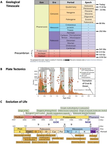
The planet Earth, our beautiful hometown, was born 4.54 billion years ago together with the birth of the Sun and the whole solar system (Holmes, 1946, 1956; Patterson, 1956), which was long after the big bang of the universe 13.8 billion years ago (Planck Collaboration, 2016). The Earth has gone through four eons: Hadean, Archean, Proterozoic and Phanerozoic (Schmitz & Ogg, 2012; Fig. 1A). Evidence from detrital zircons suggest that the Earth’s crust and oceans formed by 4.3 billion years ago (Ackerson et al., 2018; Mojzsis et al., 2001; Piani et al., 2020; Ushikubo et al., 2008; Valley et al., 2002, 2014; Watson & Harrison, 2005; Wilde et al., 2001), and there have been five major supercontinent cycles with the assembly and breakup of supercontinents Kenorland, Nuna/Columbia, Rodinia, Gondwana/Pannotia, and Pangea (Hawkesworth et al., 2016; Fig. 1B). Microfossils and other evidence indicate that the earliest life on Earth appeared 3.77–4.5 billion years ago (Betts et al., 2018; Dodd et al., 2017; Knoll & Nowak, 2017; Fig. 1C).

Fig. 1 (A) The geological timescale (adapted from image by Jonathan R. Hendricks. Image in the public domain). (B) History of Earth’s crust and plate tectonics (from Hawkesworth et al., 2016). (C) Evolution of life (from Knoll & Nowak, 2017).

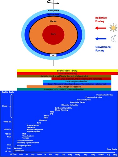
In a sphere shape, the Earth has a well-defined four-layer structure, including the atmosphere, hydrosphere, mantle and core (Fig. 2). Earth’s climate refers to the state of its outer layers. The global climate system is generally defined to have five components: the atmosphere, ocean, land, sea ice and biogeochemical cycles. The basic structure of the global climate system includes the zonal-mean Hadley circulation, Ferrel circulation and polar circulation, tropical Walker circulation, stratospheric Brewer-Dobson circulation, upper ocean upwelling and gyres, deep ocean thermohaline circulation, ice sheet volume change and sea ice change, and greenhouse gas changes. The global climate system is modulated by external radiative forcing, external gravitational forcing, plate tectonics, and various internal feedbacks such as circulation-convection feedback (Byers & Braham, 1948; Lin et al., 2006, 2015; Zipser, 1977), ocean-atmosphere feedback (Bjerknes, 1969; Lin, 2007; Wallace, 1992), land-atmosphere feedback (Brooks, 1928; Dirmeyer et al., 2012; Koster et al., 2004), ice-atmosphere feedback (Imbrie & Imbrie, 1980; Saltzman et al., 1984), as well as radiative feedbacks by clouds, aerosols and carbon cycle (Bony & Dufresne, 2005; Friedlingstein et al., 2014; Lin et al., 2014; Soden & Vecchi, 2011; Webb et al., 2006). These external forcings and internal feedbacks generate a wide spectrum of significant and complex climate variability such as the supercontinent cycle (Nance et al., 1986, 2014; Worsley et al., 1982), Phanerozoic cycles (Shaviv & Veizer, 2003; Veizer et al., 2000), interglacial cycles (Hays et al., 1976; Past Interglacials Working Group of PAGES, 2016; Raymo, 1997), millennial Heinrich/Dansgaard–Oeschger/Bond events (Bond et al., 2001; Dansgaard et al., 1993; Heinrich, 1988), Atlantic Multi-decadal Oscillation (Enfield et al., 2001; Schlesinger & Ramankutty, 1994), Pacific Decadal Oscillation/Interdecadal Pacific Oscillation (Zhang et al., 1997), El Nino-Southern Oscillation (Bjerknes, 1969), seasonal monsoons, intraseasonal Madden-Julian Oscillation (Madden & Julian, 1971), convectively coupled equatorial waves (Wheeler & Kiladis, 1999) and diurnal variation, as well as disastrous extremes such as droughts, floods, heat waves, tropical cyclones, winter blizzards, thunderstorms and tornadoes (Fig. 2).

Fig. 2 (Upper) The Earth system with external forcings and internal climate feedbacks. (Lower) Dominant variability and disastrous extremes of Earth’s climate system.

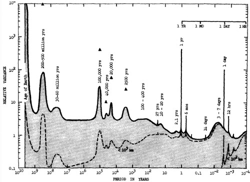
Traditionally, geological sciences often focus on thousands to billion years before the present (e.g. Gradstein et al., 2004; Holmes, 1947, 1960; Schmitz & Ogg, 2012), while atmospheric sciences generally focus on the recent centuries (e.g. IPCC, 1990, 1995, 2001, 2007, 2013; U.S. Committee for the Global Atmospheric Research Program, 1975), but a unified picture of the Earth’s climate history is desired. Kutzbach and Bryson (1974) first presented a variance spectrum of temperature fluctuations on time scales from 1 to 10,000 years from a combination of botanical, chemical, historical and instrumental records from locations in the North Atlantic sector. Mitchell (1976) presented a variance spectrum of climatic variability that spans all time scales from about one hour (10⁻⁴ years) to the age of the Earth (Fig. 3). However, observations were quite limited at that time, with the interglacial cycles just discovered in that year (Hays et al., 1976). Mitchell stated that “it is to be emphasized that the spectrum portrayed there is little more than an educated guess as to many details shown, especially those for periods longer than l0⁵ years. The most that I would wish to claim for the veracity of Fig. 1 is (1) that spectral peaks appear to belong everywhere that they are shown in Fig. 1, whether or not they are shown correctly as to relative shape, magnitude, and width; (2) that the spectrum between periods of 10 and l0⁵ years is consistent with the general picture of Quaternary climatic history published in Fig. A.2 of U.S. Committee for GARP (1975); and (3) that the spectrum for periods shorter than 10 years is consistent with instrumental observations of atmospheric variability in the twentieth century (see, e.g. Griffith et al., 1956)”. Later studies on the spectra of different timescales often focused on the shape of the background continuum (Ditlevsen et al., 2020; Franzke et al., 2020; Huybers & Curry, 2006; Lovejoy, 2015; Nilsen et al., 2016; Paillard, 2001; Pelletier, 1997; Shao & Ditlevsen, 2016; von der Heydt et al., 2021; Williams et al., 2017; Wunsch, 2003).

Fig. 3 Estimated relative variance of climate over all periods of variation (from Mitchell, 1976).

This paper reviews the observations of Earth’s climate history from 4.5 billion years to one minute with emphasis on surface temperature, sea level, and atmospheric carbon dioxide. These variables are the common topics of palaeoclimate research at different timescales and have the largest number of observational datasets. Among them, surface temperature has the largest number of observations across all timescales, followed by sea level, and atmospheric carbon dioxide. Other important variables, such as precipitation and wind circulation, are more difficult to derive from palaeoclimate proxies and do not have complete coverage for different timescales. Therefore, in this paper, we will focus on surface temperature, sea level, and atmospheric carbon dioxide. Section 2 will review the palaeoclimate proxies. Section 3 will review Earth’s surface temperature history. Section 4 will review Earth’s sea-level history. Section 5 will review Earth’s CO₂ history. For each variable, we will zoom in from Precambrian starting 4.54 billion years (Ga) ago to the current Phanerozoic eon staring 541 million years (Ma) ago and the Cenozoic era staring 66 Ma ago, to the current Quaternary period starting 2.6 Ma ago and the last glacial cycle starting 110 thousand years (ka) ago, to the current Holocene epoch starting 11.8 ka ago and the past two millennia, to the past 140 years with modern instrument records available, and to sub-annual to diurnal variations. Summary and discussions will be given in Section 6.

2 Palaeoclimate proxies

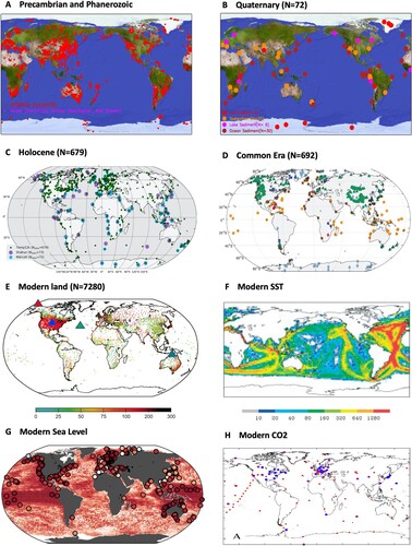
Fig. 4 summarizes the methods for observing Earth’s climate and weather. Palaeoclimatology began in the seventeenth century but started to flourish in the twentieth century after radioisotopic dating and stable isotope analysis were developed. Robert Hooke (1635–1703) is sometimes regarded as the first scientist in palaeoclimatology (Schwartzbach, 1963). Hooke observed giant turtles and oversized ammonites in the Portlandian (uppermost Jurassic) of Dorset in England and concluded that they indicated a once warmer climate. Stenonis (1669) set up the basic principles for stratigraphy, and Smith (1815, 1816) applied them to large-scale settings. Rutherford (1905) pioneered radioisotopic dating, and modern techniques of mass spectrometry were devised by Dempster (1918) and Aston (1919). Various palaeoclimate proxies were adopted in early- to mid-twentieth century, such as tree rings (Shvedov, 1892; Douglass, 1909; Kapteyn, 1914), ocean sediments (Kullenberg, 1947; Pfleger, 1948; Arrhenius et al., 1951; Emiliani, 1955), speleothems (Orr, 1952, 1953; Broecker et al., 1960), and ice cores (Coachman et al., 1958; Scholander et al., 1962; Langway et al., 1965; Dansgaard et al., 1969). The time periods covered by each type of proxies are shown in Fig. 4. In the past 100 years, numerous samples have been collected and analyzed, and the results have been compiled into data archives, such as the Precambrian and Phanerozoic GEOROC database and Veizer database (GEOROC, 2020; Shields & Veizer, 2002; Veizer & Prokoph, 2015; Fig. 5A), and the Quaternary, Holocene and Common Era datasets in the NOAA NCEI Palaeoclimatology data archive. The amount of data increases from Quaternary (Lisiecki & Stern, 2016; Shakun et al., 2015; Fig. 5B), to Holocene (Kaufman et al., 2020; Fig. 5C), to Common Era (PAGES 2k Consortium, 2017; Fig. 5D). After a large amount of data had accumulated, palaeoclimate field reconstructions were developed (Fritts, 1965; Stockton & Meko, 1975; Cook & Jacoby, 1977). The recent PAGES 2K consortium is the largest international effort in the history of palaeoclimatology to reconstruct the climate history of the common era (Anchukaitis & McKay, 2014; PAGES 2k Consortium, 2017), which has led to the latest continent-scale temperature reconstructions (PAGES 2k Consortium, 2013) and the first generation of palaeoclimate reanalysis (Hakim et al., 2016; Steiger et al., 2018).

Fig. 4 Observations of Earth’s climate and weather.

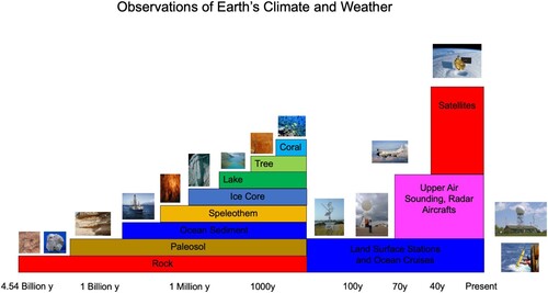
Fig. 5 Temperature records for (A) Precambrian and Phanerozoic (single, used in this study), (B) Quaternary (continuous, used in this study), (C) Holocene (from Kaufman et al., 2020), (D) Common Era (from PAGES 2k Consortium, 2017), (E) Modern land surface stations (number of years with measurements. Triangles are ARM stations. Adapted from Lawrimore et al., 2011), and (F) Modern SST (number of observations between 1880 and 1889, from Woodruff et al., 2011). (G) Modern tidal gauge stations (from Dangendorf et al., 2019). (H) Modern CO₂ stations with flask (red) and continuous (blue) measurements (from Ciais et al., 2014).

Table 1 lists the major palaeoclimate temperature datasets. There are many methods for temperature reconstruction, such as d¹⁸O, d³⁰Si, dH, TEX-86, Alkenone, Mg/Ca and Sr/Ca. SST is often derived using Alkenone and Mg/Ca methods. The alkenone-derived palaeotemperature estimates are based on the conversion of the abundance ratios of long-chain unsaturated alkenones with two to three double bonds into SST (Muller et al., 1998). The alkenone SST proxy accuracy and precision has been internationally calibrated and standardized amongst 24 laboratories worldwide (Rosell-Mele et al., 2001). The Mg/Ca ratio measured on surface-dwelling planktonic foraminifera is a well-established SST proxy that has been internationally calibrated by 25 laboratories (Greaves et al., 2008; Rosenthal et al., 2004). Temperature over land is often estimated using stable isotopic proxies. The d¹⁸O measurements provide excellent palaeotemperature records (Dansgaard, 1964; Rozanski et al., 1992, 1993; Urey, 1947), and are converted to temperature through regional empirical scales for ocean sediments (Bemis & Spero, 1998; Duplessy et al., 2002; Epstein et al., 1953; Shackleton, 1974), Greenland ice cores (Alley, 2000; Cuffey et al., 1995; Dahl-Jensen et al., 1998; Johnsen et al., 1995; Kindler et al., 2014), Antarctica ice cores (Graf et al., 2002), tropical ice cores (Thompson et al., 2000; Yao et al., 1996; Yu et al., 2021), tropical and mid-latitude speleothem cores (Dorale et al., 1998; Lachniet, 2009; Mangini et al., 2005), and lake sediments (Leng & Marshall, 2004; Stansell et al., 2017; von Grafenstein et al., 1999). dH is often used for the Antarctica ice cores (Jouzel et al., 2007), and d³⁰Si is often used for deriving Precambrian temperature.

Table 1. Palaeoclimate temperature datasets used in this study.

Region (abbrevition)	Project/site	Material	Method	Reference
Global (GLB)	Precambrian	Cherts	d30Si	Robert and Chaussidon (2006) Andre et al. (2006) van den Boorn et al. (2007) Steinhoefel et al. (2009) Abraham et al. (2011) Heck et al. (2011) Chakrabarti et al. (2012) Ding et al. (2017)
	Precambrian	Cherts	d18O	Tartese et al. (2017) Robert and Chaussidon (2006)
	Precambrian	Marine carbonate	d18O	Veizer and Prokoph (2015) Shields and Veizer (2002) Veizer et al. (1999)
	Precambrian	Resurrected proteins	Biological	Gaucher et al. (2008)
	Precambrian	Biological species	Biological	Schwartzman (2015)
	Phanerozoic	Marine carbonate	d18O	Verard and Veizer (2019)
	Phanerozoic	Marine carbonate	d18O	Song et al. (2019)
	Phanerozoic	Ocean sediment	d18O	Westerhold et al. (2020)
	Cenozoic	Ocean sediment	d18O	Mudelsee et al. (2014)
	Cenozoic	Ocean sediment	d18O	Cramer et al. (2009)
	Cenozoic	Ocean sediment	d18O	Huang et al. (2007)
	Cenozoic	Ocean sediment	d18O	Zachos et al. (2001)
	Quaternary	Ocean sediment	Model	Stap et al. (2016)
	Quaternary	Ocean sediment	Alkenone Mg/Ca	Shakun et al. (2015)
	Quaternary	Ocean sediment	d18O	Waelbroeck et al. (2002)
	Holocene	Multiple	Multiple	Kaufman et al. (2020)
	Holocene	Multiple	Multiple	Marcott et al. (2013)
	Common Era	Multiple	Multiple	PAGES 2k Consortium (2013)
	Common Era	Coral	Multiple	Tierney et al. (2015)
Northern Hemisphere (NH)	Quaternary	Ocean sediment	Model	de Boer et al. (2014)
	Common Era	Tree Ring		Guillet et al. (2017)
	Common Era	Tree Ring		Wilson et al. (2016)
	Common Era	Tree Ring		Schneider et al. (2015)
	Common Era	Multiple	Multiple	Ljungqvist (2010)
	Common Era	Multiple	Multiple	Mann et al. (2009)
	Common Era	Multiple	Multiple	Moberg et al. (2005)
	Common Era	Tree ring	Multiple	Esper et al. (2002)
	Common Era	Multiple	Multiple	Briffa (2000)
Continental Mean	Europe	Tree Ring		Luterbacher et al. (2016)
	Asia	Tree Ring		Cook et al. (2013)
	North America	Tree Ring		Trouet et al. (2013)
	South America	Multiple
	Australia	Multiple		Gergis et al. (2016)
	Arctic Antarctica	Multiple Multiple		Werner et al. (2018)
Antarctica (ANT)	EPICA Dome C	Ice core	dH	EPICA Community Members (2010)
	Vostok	Ice core	dH	EPICA Community Members (2010)
	EDML	Ice core	d18O	EPICA Community Members (2010)
	TALDICE	Ice core	d18O	Stenni et al. (2011)
	WAIS	Ice core	d18O	Steig et al. (2013)
Arctic (ARC)	NGRIP	Ice core	d18O	NGRIP Community Members (2004)
	GISP2	Ice core	d18O	Alley (2000)
	GRIP	Ice core	d18O	Vinther et al. (2010)
Africa (AFR)	Lake Malawi	Lake sediment	TEX86	Johnson et al. (2016)
	Kilimanjaro	Ice core	d18O	Thompson et al. (2002)
	Cold Air Cave	Speleothem	d18O	Holmgren et al. (1999)
	Lake Bosumtwi	Lake sediment	d18O	Shanahan et al. (2009)
	Dante Cave	Speleothem	d18O	Voarintsoa et al. (2016)
Asia (ASIA)	Sanbao Cave	Speleothem	d18O	Cheng et al. (2016)
	Borneo	Speleothem	d18O	Carolin et al. (2013)
	Borneo	Speleothem	d18O	Meckler et al. (2012)
	Soreq Cave	Speleothem	d18O	Grant et al. (2012)
	Soreq Cave	Speleothem	d18O	Bar-Matthews et al. (2003)
	Guliya	Ice core	d18O	Thompson et al. (1997)
	Dongge Cave	Speleothem	d18O	Yuan et al. (2004)
	Kesang Cave	Speleothem	d18O	Cheng et al. (2016)
	Tonnelnaya cave	Speleothem	d18O	Cheng et al. (2016)
Australia (AUS)	Cave KNI-51	Speleothem	d18O	Denniston et al. (2017)
	Mt. Arthur	Speleothem	d18O	Hellstrom et al. (1998)
	New Zealand	Speleothem	d18O	Williams et al. (2010)
Europe (EUR)	Cueva de Asiul	Speleothem	d18O	Smith et al. (2016)
	Spannagel Cave	Speleothem	d18O	Fohlmeister et al. (2013)
	Ammersee	Lake sediment	d18O	von Grafenstein et al. (1999)
	Lake Nuudsaku	Lake sediment	d18O	Stansell et al. (2017)
North America (NAM)	Devils Hole	Speleothem	d18O	Landwehr et al. (2011)
	Devils Hole	Speleothem	d18O	Moseley et al. (2016)
	Leviathan	Speleothem	d18O	Lachniet et al. (2017)
	Pink Cave	Speleothem	d18O	Asmerom et al. (2007)
	Buckeye Creek Cave	Speleothem	d18O	Cheng et al. (2019)
	Lac Aurelie	Lake sediment	d18O	Bajolle et al. (2018)
	Alaska lakes	Lake sediment	Midge	Clegg et al. (2011)
	North America	Pollen	Pollen	Viau et al. (2006)
South America (SAM)	Botuverá Cave	Speleothem	d18O	Cruz et al. (2005)
	Santiago Cave	Speleothem	d18O	Mosblech et al. (2012)
	Huascarán	Ice core	d18O	Thompson et al. (1995)
	Sajama	Ice core	d18O	Thompson et al. (1998)
	Laguna Pumacocha	Lake sediment	d18O	Bird et al. (2011)
	Cascayunga Cave	Speleothem	d18O	Wang et al. (2017)
Indian Ocean (IND)	ODP722	Ocean sediment	Alkenone	Herbert et al. (2010)
	SO189	Ocean sediment	Mg/Ca	Mohtadi et al. (2014)
Tropical Western Pacific (TWP)	ODP806B	Ocean sediment	Mg/Ca	Medina-Elizalde and Lea (2005)
	ODP1145	Ocean sediment	Mg/Ca	Oppo and Sun (2005)
	MD81	Ocean sediment	Mg/Ca	Stott et al. (2004)
	Borneo	Speleothem	d18O	Carolin et al. (2016)
Tropical eAstern Pacific (TEP)	ODP846	Ocean sediment	Alkenone	Herbert et al. (2010)
	TR163-22	Ocean sediment	Mg/Ca	Lea et al. (2006)
	ME0005A-24JC	Ocean sediment	Alkenone	Dubois et al. (2014)
	ME0005A-24JC	Ocean sediment	Alkenone	Kienast et al. (2006)
	RC11-238	Ocean sediment	Alkenone	Koutavas and Sachs (2008)
	KN176-2	Ocean sediment	Alkenone	Pahnke et al. (2007)
Northwestern Pacific (NWP)	MD882	Ocean sediment	Alkenone	Martínez-Garcia et al. (2010)
	MD01-2421	Ocean sediment	Alkenone	Yamamoto et al. (2005)
	MD01-2421	Ocean sediment	d18O	Oba and Murayama (2004)
	MD01-2412	Ocean sediment	Alkenone	Harada et al. (2006)
	IDOP U1429	Ocean sediment	Mg/Ca	Clemens et al. (2018)
Southwestern Pacific (SWP)	MD97-2120	Ocean sediment	Mg/Ca	Pahnke et al. (2003)
Northeastern Pacific (NEP)	ODP1020	Ocean sediment	Alkenone	Herbert et al. (2001)
	ODP1012	Ocean sediment	Alkenone	Herbert et al. (2001)
	ODP1019	Ocean sediment	Alkenone	Barron et al. (2003)
Southeastern Pacific (SEP)	ODP1233	Ocean sediment	Alkenone	Kaiser et al. (2005)
North Atlantic (NAO)	ODP982	Ocean sediment	Alkenone	Lawrence et al. (2009)
	MD01-2443	Ocean sediment	Alkenone	Martrat et al. (2007)
	SU8118 and MD952042	Ocean sediment	Alkenone	Bard (2002)
	MD952042	Ocean sediment	d18O	Shackleton et al. (2000)
	MD99-2275	Ocean sediment	Alkenone	Sicre et al. (2008)
TROPICAL Atlantic (TAO)	ODP662	Ocean sediment	Alkenone	Herbert et al. (2010)
	MD03-2707	Ocean sediment	Mg/Ca	Weldeab et al. (2007)
	GeoB3129/3911	Ocean sediment	Mg/Ca	Weldeab et al. (2006)
	M35003-4	Ocean sediment	Alkenone	Ruehlemann et al. (1999)
	ODP658C	Ocean sediment	Alkenone	Zhao et al. (1995)
South Atlantic (SAO)	ODP1090	Ocean sediment	Alkenone	Martínez-Garcia et al. (2010)
	MD02-2594	Ocean sediment	Mg/Ca	Dyez et al. (2014)

Table 2 lists the major palaeoclimate sea level and CO₂ datasets. Sea level can be estimated from shoreline markers, reefs and atolls, oxygen isotopes, Sr isotopes, borehole drilling, sequence stratigraphy, and palaeogeographic maps. CO₂ concentrations can be retrieved using ice cores, stomata, marine carbon isotopes, palaeosols, phytoplankton, liverworts, boron-d¹¹B, boron-B/Ca, nahcolite, calcified cyanobacteria, aeronomical evidence, and data-driven biogeochemical models. Table 3 lists the modern instrument datasets for surface temperature, sea level and CO₂. The global maps of stations are shown for land surface temperature observations (Fig. 5E, Lawrimore et al., 2011), sea surface temperature observations (Fig. 5F, Woodruff et al., 2011), tidal gauge stations (Fig. 5G, Dangendorf et al., 2019), and surface CO₂ stations (Fig. 5H, Ciais et al., 2014).

Table 2. Palaeoclimate sea level and CO₂ datasets used in this study.

Variable	Material/method	Reference
Sea Level	Precambrian d87Sr/86Sr Phanerozoic Sea Level Datasets Quaternary Sea Level Datasets Holocene Sea Level Datasets	Shields and Veizer (2002) Veizer et al. (1999) GEOROC Miller et al. (2020) Verard et al. (2015) Miller (2005) Hallam (1989) Exxon (1988) Haq et al. (1987) Spratt and Lisiecki (2016) Shakun et al. (2015) de Boer et al. (2014) Grant et al. (2014) Bintanja et al. (2005) Lea et al. (2002) Waelbroeck et al. (2002) Grant et al. (2012) Arz et al. (2007) Siddall et al. (2003) Lambeck et al. (2014) Angulo et al. (1997) Kopp et al. (2016) Kemp et al. (2018)
CO2	Precambrian CO2 Datasets Phanerzoic CO2 Datasets Quaternary and Holocene CO2 Datasets	Sheldon (2006) Mitchell and Sheldon (2010) Sheldon and Tabor (2009) Kaufman and Xiao (2003) Rye et al. (1995) Hessler et al. (2004) Kah and Riding (2007) Lichtenegger et al. (2010) Schrag et al. (2013) Royer (2014) Berner (2006) Petit et al. (1999) Beerling and Royer (2011) Zhang et al. (2013) Foster et al. (2017) Bereiter et al. (2015) Bauska et al. (2021) Ahn and Brook (2008) Kawamura et al. (2003) Barnola et al. (1987) Lisiecki (2010) Bereiter et al. (2012) Smith et al. (1997) McElwain et al. (2002) Kouwenberg (2004) Ahn et al. (2012) Indermuhle et al. (1999) Oyabu et al. (2020) Meinshausen et al. (2017)

Table 3. Modern instrument datasets used in this study.

Variables	Datasets	Time Period	Reference
Land-Ocean Surface Temperature	National Aeronautics and Space Administration (NASA) Goddard Institute for Space Studies (GISS) Hadley Center/Climatic Research Unit (HadCRUT) National Oceanic and Atmospheric Administration (NOAA) National Center for Environmental Information (NCEI)	1880–2016 1880–2016 1880–2016	Hansen et al. (2010) Morice et al. (2012) Vose et al. (2012)
Sea Surface Temperature	International Comprehensive Ocean Atmosphere Data Set (ICOADS) Extended Reconstructed Sea Surface Temperature (ERSST) Version 4 Hadley Centre Sea Surface Temperature (HadSST3) Hadley Centre Sea Ice and Sea Surface Temperature (HadISST1) Centennial In Situ Observation-Based Estimates (COBE2)	1880–2016 1880–2016 1880–2016 1880–2016 1880–2016	Freeman et al. (2017) Huang et al. (2015) Kennedy et al. (2011) Rayner et al. (2003) Hirahara et al. (2014)
Surface Air Temperature	Global Historical Climatology Network (GHCN) Climatic Research Unit Surface Air Temperature High Resolution (CRUTS) University of Delaware Surface Air Temperature (UDEL) Atmospheric Radiation Measurement (ARM) Stations One-Minute Data	1880–2016 1901–2014 1900–2014 2016–2017	Lawrimore et al. (2011) Harris et al. (2014) Willmott and Robeson (1995) Stokes and Schwartz (1994)
CO2	All surface stations Mauna Loa AIRS/Aqua satellite Aircraft measurements Chemical methods	1965–2016 1959–2016 2003–2016 2004–2016 1812–1963	https://airs.jpl.nasa.gov/data/carbon_dioxide Beck (2007)
Global Sea Level from Tidal Gauge Stations	Permanent Service for Mean Sea Level (PSMSL) dataset for 2200 tidal stations around the world Global Extreme Sea Level Analysis (GESLA) dataset Global sea level reconstructions	1806–Now 1806–Now 1900–2018 1900–2015 1900–2010 1808–2009 1880–2013 1900–2007	Holgate et al. (2013) link Woodworth et al. (2017) Frederikse et al. (2020) Dangendorf et al. (2019) Hay et al. (2015) Jevrejeva et al. (2014) Church and White (2011) Ray and Douglas (2011)
Global Sea Level from Satellite Measurements	NASA AVISO University of Colorado	1993–2016 1993–2016 1993–2016	https://podaac-ftp.jpl.nasa.gov/dataset/MERGED_TP_J1_OSTM_OST_GMSL_ASCII_V4 https://www.aviso.altimetry.fr/en/data/products/ocean-indicators-products/mean-sea-level.html http://sealevel.colorado.edu

Dating plays a key role in palaeoclimate studies. Some of the proxies, such as tree rings, ice cores, coral reefs and speleothems, have natural annual layers, allowing accurate dating using annual layers counting up to 40 ka. Several time scales have been developed for Greenland and Antarctica ice cores, such as the Greenland Ice Core Chronology 2005 (GICC05) (Andersen et al., 2006; Rasmussen et al., 2006, 2008; Svensson et al., 2006, 2008; Vinther et al., 2006), the NEEM ice core chronology (Rasmussen et al., 2013), the INTIMATE event stratigraphy (Rasmussen et al., 2014), the Antarctic ice core chronology (AICC2012) (Bazin et al., 2013; Veres et al., 2013), the WAIS Divide deep ice core WD2014 chronology (Buizert et al., 2015; Sigl et al., 2016), and the South Pole ice core SP19 chronology (Winski et al., 2019). Bipolar synchronization has been realized (Lemieux-Dudon et al., 2010; Veres et al., 2013). However, manual layer counting is a tedious and sometimes subjective method. The GICC05 chronology was developed over several years and involved the efforts of many researchers: counting, comparing, and recounting the annual layers recorded in multiple data records from several Greenland ice cores. Automated counting approaches are being developed (Wheatley et al., 2012; Winstrup et al., 2012). For the speleothems, most of the cores were radiometrically dated and a global speleothem isotope database with multiple age-depth models is being developed (Comas-Bru et al., 2020). Ocean sediment cores are difficult to date precisely (see review by Lisiecki & Stern, 2016). Radiocarbon offers relatively good age control for the last 40 ka but is costly and can still have calendar age uncertainties of more than 1000 years due to calibration and reservoir age uncertainty. Beyond 40 ka, sediment cores are generally dated by correlating a palaeoclimate proxy to either a better-dated climate archive (e.g. ice cores or speleothems) or to changes in Earth’s orbital configuration (i.e. “orbital tuning”). These dating methods assume that the ocean sediment records are in phase with the target archive or orbital configuration, but in reality, there may exist a physical time lag. Raymo (1997) demonstrated an absolute “constant sedimentation rate” timescale using radiometric age constraints. Significant advances have been made in developing the global ocean sediment timescales (Imbrie et al., 1984; Lisiecki & Raymo, 2005; Lisiecki & Stern, 2016; Shackleton & Opdyke, 1973).

3 Earth’s surface temperature history

Earth’s temperature history at billion-year timescales has been examined by many studies using zircon and quartz in earliest rocks (Ackerson et al., 2018; Valley et al., 2002; Watson & Harrison, 2005), oxygen isotope from cherts and phosphates (Blake et al., 2010; Hren et al., 2009; Karhu & Epstein, 1986; Knauth, 2005; Knauth & Epstein, 1976; Knauth & Lowe, 1978, 2003), marine carbonate isotope (Prokoph et al., 2008; Shields & Veizer, 2002), silicon isotopes in cherts (Abraham et al., 2011; Andre et al., 2006; Chakrabarti et al., 2012; Ding et al., 2017; Heck et al., 2011; Marin-Carbonne et al., 2012; Robert & Chaussidon, 2006; Steinhoefel et al., 2009; van den Boorn et al., 2007), resurrected proteins (Gaucher et al., 2008), and upper-temperature limits for growth of living organisms (Schwartzman, 2015). For the Hadean eon (4.5–4.0 billion years ago), Watson and Harrison (2005) discovered using ancient zircons from Western Australia's Jack Hills that Earth’s surface temperature has cooled down to about 700°C, while Ackerson et al. (2018) found that quartz crystals in Tuolumne samples record crystallization temperatures of 474–561°C. For the Archean, Proterozoic and Phanerozoic eons, Knauth and Epstein (1976) made the first estimate of temperature using oxygen isotope from cherts and suggested that the average climatic temperatures reached about 70°C at 3 Ga, decreased to about 52°C at 1.3 Ga, decreased from about 34°C to 20°C through the Palaeozoic, increased to 35–40°C in the Triassic, and then decreased through the Mesozoic to Tertiary values of about 17°C (Fig. 6A). Robert and Chaussidon (2006) analyzed silicon isotopes in cherts and suggested that seawater temperature changes from about 70°C at 3.5 Ga to about 20°C at 0.8 Ga, but with much larger variability than that derived from oxygen isotopes (Fig. 6B). Gaucher et al. (2008) used resurrected proteins to infer Precambrian temperature and suggested that temperature cooled down from about 72°C at 3.6 Ga to 39°C at 0.8 Ga. Hren et al. (2009) did a combined analysis of oxygen and hydrogen isotopes in cherts and suggested that the Archean temperature at 3.42 Ga. was below 40°C. This low Archean temperature scenario was supported by Blake et al. (2010), who examined oxygen isotopes in phosphate and found a sea water temperature between 26°C and 35°C in 3.2–3.5 Ga, which is close to today’s temperature.

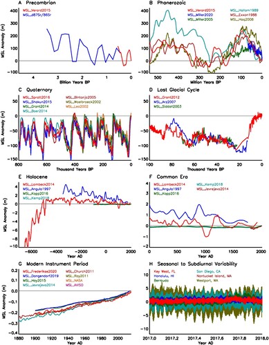
Fig. 6 (A) Precambrian temperature derived from oxygen isotope and silicon isotope in cherts (from Tartèse et al., 2017). (B) Phanerozoic temperature derived from marine oxygen isotope (from Veizer & Prokoph, 2015). (C) Quaternary SST from the individual (cyan) and stacked (blue) records (from Shakun et al., 2015). (D) Late Quaternary temperature from Greenland and Antarctica ice cores (from EPICA Community Members, 2006). (E) Common Era northern hemisphere mean surface temperature (from IPCC, 2013). (F) Modern global mean surface temperature anomalies (from IPCC, 2013).

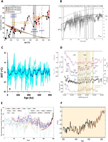
The Phanerozoic temperature history has been studied using oxygen isotopes in carbonates and phosphates (Cramer et al., 2009; Grossman, 2012; Mills et al., 2019; Prokoph et al., 2008; Royer et al., 2004; Scotese et al., 2021; Shaviv et al., 2014; Shaviv & Veizer, 2003, 2004; Veizer et al., 1999, 2000; Veizer & Prokoph, 2015). Veizer and Prokoph (2015) found that the sea water temperature was about 30°C above today’s value at 480 Ma, which shows a general cooling trend since then but with significant variability (Fig. 6C). Oscillations with an amplitude of about 5–10°C were reported. Veizer et al. (2000) found a prominent ∼140 Ma oscillation, which was connected to the oscillation of galactic cosmic ray flux (Shaviv & Veizer, 2003). Shaviv et al. (2014) reported a significant 32 Ma oscillation with a secondary 175 Ma frequency modulation, which is consistent with parameters postulated for the vertical motion of the solar system across the galactic plane, modulated by the radial epicyclic motion.

The Cenozoic temperature history has been analyzed using ocean sediments (Cramer et al., 2009; Friedrich et al., 2012; Lear et al., 2000; Miller et al., 1987; Miller et al., 2020; Mudelsee et al., 2014; Shackleton & Kennett, 1975; Westerhold et al., 2020; Zachos et al., 2001), and continental sediments (Mosbrugger et al., 2005). All proxies consistently show a long-term cooling of 10–20°C in deep ocean and over the continents throughout the Cenozoic. On top of the strong cooling trend, Zachos et al. (2001) found rhythmic or periodic cycles driven by orbital processes with 10⁴- to 10⁶-year cyclicity and rare rapid aberrant shifts and extreme climate transients with durations of 10³–10⁵ years. Westerhold et al. (2020) identified four climate states-Hothouse, Warmhouse, Coolhouse, Icehouse-on the basis of their distinctive response to astronomical forcing depending on greenhouse gas concentrations and polar ice sheet volume.

The Quaternary temperature history has been examined by many studies using ocean sediments (Emiliani, 1955; Hays et al., 1976; Imbrie et al., 1973; Imbrie et al., 1984; Lisiecki & Raymo, 2005; Martinson et al., 1987; Raymo, 1997; Shackleton et al., 1990; Shackleton & Opdyke, 1973; Shakun et al., 2015; Waelbroeck et al., 2002; Zachos et al., 2001), ice cores (Petit et al., 1999; Alley, 2000; EPICA Community Members, 2004, 2006; NGRIP Members, 2004; Vinther et al., 2010; Jouzel, 2013), lake sediments (Camuera et al., 2019; Tzdakis et al., 1997), and speleothem (Carolin et al., 2013; Cheng et al., 2016; Johnson et al., 2016; Lachniet et al., 2017; Landwehr et al., 2011). The interglacial cycles were first discovered in ocean sediment cores (Emiliani, 1955; Imbrie et al., 1973). Shackleton and Opdyke (1973) proposed the formalization of Marine Isotope Stages (MIS) 1–22, using the d18O in foraminifera in core V28–238 from the Eastern Equatorial Pacific, a practice which has been gradually extended over the entire Pleistocene, Pliocene and beyond in later timescales such as Imbrie et al. (1984) and Lisiecki and Raymo (2005). Hays et al. (1976) proposed that the interglacial cycles are linked to the Milankovitch cycles – the eccentricity (100,000 year), obliquity (41,000 year) and precession (23,000 year) cycles of Earth’s orbit (Milankovitch, 1941). Raymo (1997) confirmed the relationship using an untuned constant sedimentation rate timescale. Ice cores from Antarctica and Greenland show similar cycles (EPICA Community Members, 2004, 2006; Petit et al., 1999). By data compilations, Past Interglacials Working Group of PAGES (2016) showed that despite spatial heterogeneity, MIS 5e (last interglacial) and 11c (∼400 ka ago) were globally strong (warm), while MIS 13a (∼500 ka ago) was cool at many locations. A step-change in the strength of interglacials at 450 ka is apparent only in the Antarctic and deep ocean temperature. The range of temperature variation is about 3°C for the global ocean mean but could be as large as 14°C at individual ocean locations and 20°C in Greenland (Alley, 2000; Shakun et al., 2015; Fig. 6C). The dominant oscillation period is about 100,000 years in the recent 1 Ma but 41,000 years before (Lisiecki, 2010). The interglacial cycles over land are often different from those in oceans and polar regions. Using pollen records from Europe, Tzdakis et al. (1997) showed that the terrestrial cycles have stronger high-frequency variability. Using speleothem records from China, Cheng et al. (2016) found strong precession cycles rather than eccentricity cycles in the past 640,000 years.

The temperature history of the last glacial cycle has been studied using ice cores (Dansgaard et al., 1971; EPICA Community Members, 2006; Jouzel et al., 2007; NGRIP Members, 2004; Thompson et al., 1997), speleothem (Carolin et al., 2013; Cheng et al., 2019; Cruz et al., 2005; Lachniet et al., 2017; Mosblech et al., 2012; Wang et al., 2001), lake sediments (van der Hammen et al., 1971; Woillard, 1978), and ocean sediments (Bard, 2002; Cacho et al., 1999; Dyez et al., 2014; Harada et al., 2006; Hodell et al., 2010; Kaiser et al., 2005; Lea et al., 2000; Lisiecki & Stern, 2016; Martrat et al., 2007; Mohtadi et al., 2014; Sancetta et al., 1973; Schulz et al., 1998; Shackleton et al., 2000; Vautravers & Shackleton, 2006; Voelker et al., 2006; Voelker & de Abreu, 2011). Millennial-scale oscillations have been discovered, such as the Heinrich events (Heinrich, 1988), the Dansgaard–Oeschger (D–O) events (Dansgaard et al., 1993) and the Antarctica Isotope Maximum (AIM) events (EPICA Community Members, 2006; Fig. 6D). The Heinrich events have an oscillation period of 6000–10,000 years, while the DO and AIM events have an oscillation period of 1000–2000 years. Greenland has the strongest temperature anomalies of ∼10°C associated with the Heinrich and DO events. Antarctica has clear but weaker anomalies of ∼2–4°C. There is an SST anomaly of ∼5°C in North Atlantic (Bard, 2002; Shackleton et al., 2000), ∼2°C in the South Atlantic (Dyez et al., 2014), ∼1°C in the Indian Ocean (Mohtadi et al., 2014; Schulz et al., 1998), ∼5°C in Northwest Pacific (Harada et al., 2006), and ∼2°C in Southeast Pacific (Kaiser et al., 2005). Lisiecki and Stern (2016) compiled stacked records for each ocean basin and the global oceans. Over land, there are temperature anomalies of 2–6°C in Asia (Carolin et al., 2013; Cheng et al., 2016; Wang et al., 2001), South America (Cruz et al., 2005; Mosblech et al., 2012) and North America (Cheng et al., 2019; Lachniet et al., 2017).

The Holocene temperature history has been studied using lake sediments (Bajolle et al., 2018; Davis et al., 2003; Viau et al., 2006), ice cores (Thompson et al., 2000; Thompson et al., 1995; Thompson et al., 1998; Thompson et al., 2002), speleothem (Affolter et al., 2019; Asmerom et al., 2007; Fohlmeister et al., 2013; Holmgren et al., 1999; Persoiu et al., 2017; Smith et al., 2016; Stansell et al., 2017; Wang et al., 2005; Williams et al., 2010), ocean sediments (Goslin et al., 2018; Hald et al., 2007; Kim et al., 2004; Staubwasser et al., 2003), northern hemisphere reconstructions (Marsicek et al., 2018; Pei et al., 2017) and global reconstructions (Kaufman et al., 2020; Marcott et al., 2013). Many records show two distinct events: a 4.2 ka event which is most strongly recorded in proxy climate records from mid- and low latitudes, and an 8.2 ka event which is a short-lived near-global episode (Walker et al., 2019). Bond et al. (1999, 2001) discovered a millennial-scale oscillation with a period of ∼1500 years.

The Common Era temperature history has been examined by numerous studies with reconstructions of the northern hemisphere mean temperature (Briffa, 2000; Esper et al., 2002; Guillet et al., 2017; Jones et al., 1998; Mann et al., 1999, 2009; Moberg et al., 2005; Ljungqvist, 2010; Schneider et al., 2015; Wilson et al., 2016; Fig. 6E), continental mean temperature (Cook et al., 2013; Gergis et al., 2016; Luterbacher et al., 2016; PAGES 2k Consortium, 2013; Trouet et al., 2013; Werner et al., 2018), ocean basin mean temperature (Tierney et al., 2015) and local temperature (see Table 1). The Common Era temperature displays significant Medieval and Roman warm periods and Little Ice Age cold period, as well as strong multi-decadal oscillations (Fig. 6E).

Modern instrument measurements were available for the past 170 years since 1850. The global mean surface temperature has been constructed, which shows global warming of ∼1°C from 1910 to 2010 (Hansen & Lebedeff, 1987; Hansen et al., 2010; Jones et al., 1986; Morice et al., 2012; Vose et al., 2012; Fig. 6F). The global mean temperature is also affected by the AMO (DelSole et al., 2011; Tung & Zhou, 2013; Wu et al., 2011), IPO (England et al., 2014; Meehl et al., 2013, 2014), and ENSO (Fyfe et al., 2016; Trenberth, 2015).

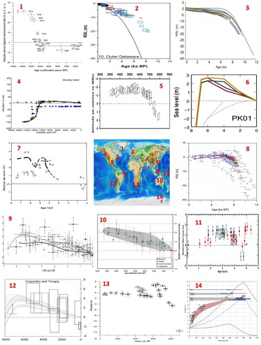
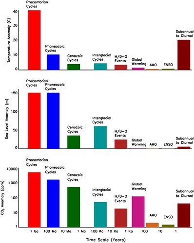
Fig. 7 summarizes Earth’s temperature history from 4.5 billion years to one minute. Precambrian temperature oscillates with the supercontinent cycle – the alternate aggregation and breakup of supercontinent (Fig. 7A), Phanerozoic temperature shows a 100–200 million year cycle (Fig. 7B), while the Quaternary temperature is dominated by the 100,000 year interglacial cycle (Fig. 7C). The late Quaternary temperature of the last glacial cycle displays millennium-scale cycles such as the Heinrich events and D–O events (Fig. 7D), while Holocene temperature shows centennial- to millennial-scale cycles (Fig. 7E). Common Era temperature is dominated by multi-decadal oscillations (Fig. 7F). For the modern instrument period (Fig. 7G), the magnitude of global warming is about 1°C century⁻¹. There are also global mean temperature signals associated with AMO and ENSO. The oscillation amplitudes decrease from billion-year time scales to centennial timescales but strongly increase at seasonal and diurnal timescales. Fig. 7H illustrates the one-minute surface temperature measurements at different latitude belts, which include seasonal cycle, diurnal cycle, and other high-frequency phenomena such as the MJO, tropical waves, mesoscale convective systems, and thunderstorms. The oscillation amplitudes range from 10–20°C over tropical and mid-latitude oceans to 40–50°C over mid-latitude and high-latitude continents. The global map of seasonal temperature ranges displays a 10°C range over tropical continents and a 20–60°C range over extratropical continents (data not shown). The diurnal temperature range is more uniform (8–16°C) around the globe except for Greenland, which has a 20+°C day-night temperature difference (not shown).

Fig. 7 Earth’s surface temperature history for (A) Precambrian, (B) Phanerozoic, (C) Quaternary, (D) late Quaternary, (E) Holocene, (F) Common Era, (G) 1880–2019, and (H) 2015 (one-minute data from the ARM stations in Fig. 5E).

Overall, Fig. 7 demonstrates three key points. First, Earth’s temperature history shows significant oscillations at all timescales. Secondly, the oscillation amplitudes decrease from 40°C to 60°C at billion-year timescale to about 1°C at interannual timescales, then strongly increase at seasonal and diurnal timescales. Oscillation amplitudes at seasonal and diurnal timescales are similar to those at billion-year timescales. Thirdly, fewer datasets and larger uncertainties exist for observations at longer timescales such as Precambrian and Phanerozoic.

4 Earth’s sea-level history

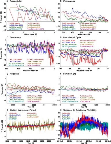
Sea level is affected by plate tectonics (sea area, dynamic topography, ridge volume, sea floor volcanism, icesheet-induced isostatic depression), ocean sediment thickness, and climate (ice volume, ocean thermal expansion, ground water) (Miller et al., 2005; Conrad, 2013; Fig. 8A, B). The Precambrian sea-level history has been studied using sequence stratigraphy (Eriksson, 1999; Eriksson et al., 1999, 2005; Krapez, 1993) and 87Sr/86Sr (Halverson et al., 2007). Krapez (1993) assessed the stratigraphic succession of the 3580–2770 m.y. old granite-greenstone terrain of the Pilbara Block by the first- and second-order sequence-stratigraphic techniques and identified two sea-level cycles associated with the Supercontinent Cycles. Halverson et al. (2007) compiled the 87Sr/86Sr records from 0 to 0.9 Ga. In this study, we extended the 87Sr/86Sr records to 0–3.5 Ga using the Veizer Precambrian and Phanerozoic databases (Shields & Veizer, 2002; Veizer et al., 1999) and the GEOROC database.

Fig. 8 (A) Physical processes contributing to sea level variation from 1 yr to 100 Ma. SF, sea floor. Cont, continent (from Miller et al., 2005). (B) Physical processes contributing to Phanerozoic sea level variation (from Conrad, 2013). (C) Phanerozoic sea-level history (from Verard et al., 2015). (D) Quaternary sea-level history (from Shakun et al., 2015). (E) Late Quaternary sea-level history based on oxygen isotope (line) and coral terraces (black circles) (from Chappell et al., 1996). (F) Modern sea level history (from IPCC, 2013).

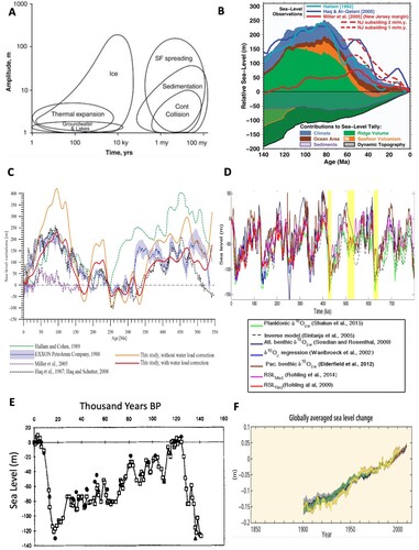
The Phanerozoic sea-level history has been examined using palaeogeographic maps (Egyed, 1956; Hallam, 1971; Hallam, 1984, 1989; Hays & Pitman, 1973; Pitman, 1978), seismic stratigraphy (Haq et al., 1987; Haq & Schutter, 2008; Posamentier & Vail, 1988; Vail et al., 1977), borehole drilling (Kominz et al., 1998; Miller et al., 1998; Miller et al., 2005; Watts & Steekler, 1979), and 87Sr/86Sr record (Francois & Walker, 1992; Montafiez et al., 1996; Verard et al., 2015). Using early palaeogeographic data, Egyed (1956) estimated that global sea level was 70 m higher than today at 350 Ma. With updated palaeogeographic maps, Hallam (1984, 1989) constructed a detailed sea-level curve for Phanerozoic. Vail et al. (1977) first developed the method of seismic stratigraphy, which uses the seismic data to derive depositional sequence, local relative sea-level change and global sea-level cycles. This led to the Exxon sea-level curve (Haq et al., 1987; Posamentier & Vail, 1988) and the Haq and Schutter (2008) curve. Watts and Steekler (1979) developed the backstripping method using borehole data, which is an inverse technique that can be used to quantitatively extract sea-level change amplitudes from the stratigraphic record. It accounts for the effects of sediment compaction, loading (the response of crust to overlying sediment mass), and water-depth variations on basin subsidence. Miller et al. (2005) derived a sea-level curve based on backstripping stratigraphy data. The 87Sr/86Sr record reflects weathering of the Earth and has been shown to be a good proxy for global sea level (Francois & Walker, 1992; Montafiez et al., 1996). Verard et al. (2015) derived a sea-level curve using 87Sr/86Sr records with consideration of the tectonics effects. The latest Phanerozoic sea-level curves are shown in Fig. 8C. The various methods produce similar “double hump” pattern, although the magnitudes of the peaks differ.

The Cenozoic sea-level history has been analyzed using higher resolution borehole and ocean sediment datasets (e.g. Kominz et al., 1998; Miller et al., 2020; Zachos et al., 1999). The Cenozoic sea-level records the evolution from an ice-free Early Eocene to Quaternary bipolar ice sheets. Miller et al. (2020) found that peak warmth, elevated global sea level, high CO₂, and ice-free “Hothouse” conditions (56–48 Ma) were followed by “Cool Greenhouse” (48–34 Ma) ice sheets (10–30 m changes). Continental-scale ice sheets (“Icehouse”) began ∼34 Ma (>50 m changes), permanent East Antarctic ice sheets at 12.8 Ma, and bipolar glaciation at 2.5 Ma. The largest global sea-level fall (27–20 ka; ∼130 m) was followed by a >40 mm yr⁻¹ rise (19–10 ka), a slowing (10–2 ka), and a stillstand until ∼1900 CE, when rates began to rise. High long-term CO₂ caused warm climates and high sea levels, with sea-level variability dominated by periodic Milankovitch cycles.

The Quaternary sea-level history has been studied using direct dating of shoreline markers and reefs (Emery & Garrison, 1967; Hails, 1965; Shepard, 1964; Shepard & Suess, 1956; Vries & Barendsen, 1954) and oxygen isotopes in ocean sediments (Emiliani, 1955; Shackleton, 1967). The two approaches can be combined together to yield accurate and high-resolution sea-level records (Chappell & Shackleton, 1986; Fairbanks, 1989). Sea level curves have been constructed for the Quaternary (de Boer et al., 2014; Bintanja et al., 2005; Grant et al., 2014; Lea et al., 2002; Shakun et al., 2015; Spratt & Lisiecki, 2016; Waelbroeck et al., 2002; Fig. 8D) and the last glacial cycle (Bard et al., 1990; Chappell et al., 1996; Grant et al., 2012; Lambeck & Chappell, 2001; Lisiecki & Stern, 2016; Siddall et al., 2003; Siddall et al., 2008; Siddall et al., 2010; Fig. 8E). The Quaternary sea-level shows a >100 m oscillation, which is mainly controlled by ice volume change associated with the interglacial cycles (Fig. 8D). Within the last glacial cycle, global sea level is affected by the Heinrich events and D–O events, and shows a 20–30 m oscillation (Fig. 8E).

The Holocene sea level history has been examined by numerous studies using radio-isotopic dating of shoreline markers and/or reef terraces in Greenland (Bennike et al., 2011; Long et al., 2003; Sparrenbom et al., 2006), Atlantic coast of U.S. (Engelhart & Horton, 2012), Atlantic coast of Europe (Garcia-Artola et al., 2018), Pacific coast of North America (Shugar et al., 2014); Pacific coast of central North America (Engelhart et al., 2015), U.S. Gulf Coast (Tornqvist et al., 2004), east coast of China (Song et al., 2013), east coast of India (Banjeree, 2000), Southeast Asia (Mann et al., 2019), Brazilian coast (Angulo & Lessa, 1997; Angulo, 2005), Australian coast (Lewis et al., 2013), Pacific islands (Rashid et al., 2014), south coast of Africa (Garrett et al., 2020), Chilean coast (Cooper et al., 2018), and Antarctica coast (Watcham et al., 2011). There was a decrease in sea level in Holocene around the world except for the North Atlantic Ocean where there was a sea-level rise (Fig. 9). Several reconstructions of global sea level have been developed (Kopp et al., 2016; Lambeck et al., 2014). The Lambeck et al. (2014) reconstruction uses mainly observations from the Pacific and Indian oceans and shows a decrease in global sea level, while the Kopp et al. (2016) reconstruction uses mainly observations from the Atlantic Ocean and shows an increase in global sea level. Regional curves have also been generated, for example, for the North Atlantic (Kemp et al., 2018) and South Atlantic (Angulo & Lessa, 1997; Angulo et al., 2005). Currently, global map of sea level is being developed for Holocene and Common Era (Horton et al., 2018; Khan et al., 2015, 2019).

Fig. 9 Holocene sea-level history in different regions from (1) Sparrenbom et al. (2006); (2) Engelhart and Horton (2012), (3) Garcia-Artola et al. (2018); (4) Shugar et al. (2014); (5) Tornqvist et al. (2004); (6) Song et al. (2013); (7) Banjeree (2000); (8) Mann et al. (2019), (9) Angulo et al., 2006; (10) Lewis et al. (2013); (11) Rashid et al. (2014); (12) Garrett et al. (2020); (13) Cooper et al. (2018); (14) Watcham et al. (2011). World map courtesy of NOAA.

Modern measurements of ocean tides and global sea level began in the mid-seventeenth century using float tide gauges (Matthaus, 1972). The first generation of self-recording tide gauges was developed in the 1830s by Palmer, Mitchell, Bunt and others (Palmer, 1831; Matthaus, 1972). Since then, many tidal gauge stations have been set up around the world. The Permanent Service for Mean Sea Level of the UK National Oceanography Center was established in 1933 and has been collecting global sea level measurements till now (Holgate et al., 2013). Now the longest continuous tide record and global sea-level reconstruction go back to 1700 (van Veen, 1945). Starting from 1991, satellite measurements of sea surface height has been available from TOPEX/Poseidon, Jason-1, Jason-2, ERS-1, ERS-2, Envisat and other platforms (Ablain et al., 2015; GSFC, 2017; Nerem et al., 2018). Global tidal models have been developed and calibrated by the observations (e.g. Egbert & Erofeeva, 2002). Reconstructions of global sea level have been developed for 1807-now from the gauge records with the help of recent satellite measurements and tidal models (e.g. Jevrejeva et al., 2006; Jevrejeva et al. 2014; Jevrejeva et al. 2008; Merrifield et al., 2009; Church & White, 2011; Ray & Douglas, 2011; Dangendorf et al., 2019).

In summary, the global sea level also demonstrates significant oscillations at different timescales (Fig. 10). Precambrian sea level oscillates dramatically with supercontinent cycles with an amplitude of 100–200 m (Fig. 10A), while Phanerozoic sea level also shows a 100–200 m oscillation (Fig. 10B). Quaternary sea level displays the well-known 100-m oscillation associated with global interglacial cycle (Fig. 10C), and sea level in the last glacial cycle shows 10–50 m oscillation associated with the millennium-scale Heinrich and D–O events (Fig. 10D). The amplitudes decrease substantially to about 1 m for Holocene sea level (Fig. 10E) and 0.1 m for Common Era sea level (Fig. 10F). The modern global sea level displays a trend of ∼0.2 m century⁻¹ (Fig. 10G). There is a tendency for positive trend in low latitudes but negative trend in high latitudes (not shown). Sea level also shows decadal and interannual oscillations with amplitudes smaller than 0.5 m. The oscillation amplitudes of sea-level increase strongly at subseasonal and diurnal timescales, driven by the well-known lunar and solar tidal force. Fig. 10H illustrates the hourly measurements from coastal and island tidal gauge stations at different latitudes. Sea level rises and falls by 1–10 m everyday throughout the year, which is contributed by all constituents of tidal force as well as surface winds. The largest tidal constituent – the semi-diurnal lunar M2 tide, has a >0.4 m oscillation around most coastal regions (Egbert et al., 2002).

Fig. 10 Earth’s sea-level history for (A) Precambrian, (B) Phanerozoic, (C) Quaternary, (D) late Quaternary, (E) Holocene, (F) Common Era, (G) 1880–2019, and (H) 2017 (hourly data from tidal gauge stations).

5 Earth’s atmospheric CO₂ history

Precambrian CO₂ history has been studied using various proxies such as palaeosols, calcified cyanobacteria and aeronomical evidence (Rye et al., 1995; Kaufman & Xiao, 2003; Hessler et al., 2004; Sheldon, 2006; Kah & Riding, 2007; Sheldon & Tabor, 2009; Mitchell & Sheldon, 2010; Lichtenegger et al., 2010; Driese et al., 2011; Schrag et al., 2013; Kanzaki & Murakami, 2015; Catling & Zahnle, 2020; Fig. 11A). Rye et al. (1995) analysed palaeosols from 2.75Ga and found that CO₂ concentration must be less than 10^−1.4 atm, which is about 100 times the present-day atmospheric level (PAL). Hessler et al. (2004) studied palaeosols from 3.2 Ga and found a lower limit of CO₂ concentration being several times higher than present-day values. Sheldon (2006) used a different model and found consistently high pCO2 from 2.5 to 1.8 Ga ago and a substantial drop in atmospheric pCO2 at some time between 1.8 and 1.1 Ga ago. Kah and Riding (2007) used calcified cyanobacteria between 1 and 2.5 Ga and derived CO₂ concentration that is about 10 times today’s value. Lichtenegger et al. (2010) showed aeronomical evidence of a CO₂ amount in the early nitrogen-rich terrestrial atmosphere 3.8 Ga ago of at least two orders of magnitude higher than the present-time level. Kanzaki and Murakami (2015) derived from palaeosols CO₂ concentration to be 85–510 PAL at 2.77 Ga, 78–2500 PAL at 2.75 Ga, 160–490 PAL at 2.46 Ga, 30–190 PAL at 2.15 Ga, 20–620 PAL at 2.08 Ga and 23–210 PAL at 1.85 Ga.

Fig. 11 (A) Precambrian CO₂ history from a model (black line, yellow shading indicates its 95% confidence level) and various observations (from Catling & Zahnle, 2020). (B) Phanerozoic CO₂ history from proxies (from Royer, 2014). (C) Quaternary CO₂ history from Antarctic ice core composite and temperature from EPICA (from Luthi et al., 2008). (D) Late Quaternary CO₂ history from Byrd Station, Antarctica together with other climate variables (from Ahn & Brook, 2008). (E) Common era CO₂ history from ice core measurements in Greenland (symbols) and Antarctica (line) (from Barnola et al., 1995). (F) Common era CO₂ history from ice core measurements in NEEM, Dome Fuji, Law Dome, WDC, EDML and South Pole (from Oyabu et al., 2020). (G) Common era CO₂ history from stomata (dots) and ice core (black line) (from Finsinger & Wagner-Cremer, 2009). (H) Historical CO₂ concentrations used by IPCC AR6 (from Meinshausen et al., 2017).

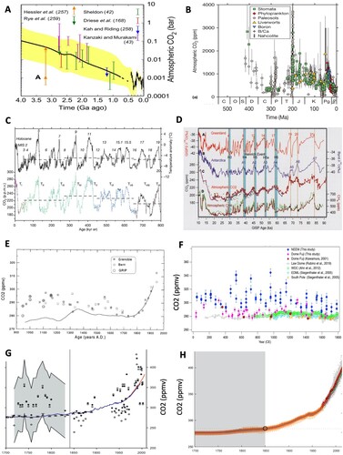
The Phanerozoic CO₂ history has been examined by numerous studies using stomata (e.g. Konrad et al., 2020; McElwain & Steinthorsdottir, 2017; van der Burgh et al., 1993), phytoplankton (e.g. Pagani et al., 1999), liverworts (Fletcher et al., 2008), palaeosols (e.g. Suchecki et al., 1988), boron-d¹¹B (Pearson et al., 2009), boron-B/Ca (Tripati et al., 2009), nahcolite (Lowenstein & Demicco, 2006), and data-driven biogeochemical models (Berner, 1991, 1994, 2006; Berner & Kothavala, 2001; Godderis et al., 2014; Rothman, 2002; Shaviv & Veizer, 2003). An increase in the atmospheric carbon dioxide (CO2) concentration results in a decrease in the number of leaf stomata, and van der Burgh et al. (1993) found a nearly perfect linear correlation between them. Pagani et al. (1999) showed a good correlation between pCO₂ and ϵ_p values based on carbon isotope analyses of diunsaturated alkenones and planktonic foraminifera. Fletcher et al. (2008) estimated ancient atmospheric CO2 concentrations on the basis of δ13C measurements on liverwort gametophyte compression fossils, which spanned 150 Ma and were sampled from 12 localities on 5 continents. Lowenstein and Demicco (2006) estimated pCO₂ from coprecipitation of nahcolite (NaHCO₃) and halite (NaCl) from surface waters in contact with the atmosphere and found a value of 1125 ppm between 49 and 56 Ma. As reviewed by Royer (2014; Fig. 11B), there is a broad agreement among methods. The Phanerozoic CO₂ history is characterized by a “double hump” pattern with elevated CO₂ around 180 and 400 Ma, both of which are above 1000 ppm. The Cenozoic CO₂ history has also been examined using higher resolution data (e.g. Beerling & Royer, 2011; Pagani et al., 2011; Pearson & Palmer, 2000; Rugenstein & Chamberlain, 2018; Steinthorsdottir et al., 2016; Zhang et al., 2013). Zhang et al. (2013) found consistent results among alkenone data, boron isotope, pH data and stomatal index records. CO₂ levels were highest during a period of global warmth associated with the Middle Miocene Climatic Optimum (17–14 Ma), followed by a decline in CO₂ during the Middle Miocene Climate Transition (approx. 14 Ma).

The Quaternary CO₂ history has been studied using ice cores (Barnola et al., 1987; Bereiter et al., 2015; Delmas et al., 1980; Kawamura et al., 2003; Luthi et al., 2008; Neftel et al., 1982; Petit et al., 1999; Fig. 11C) and marine carbon isotopes (Lisiecki, 2010). CO₂ concentration shows an ∼100 ppm oscillation associated with the interglacial cycles and is in phase with the temperature oscillation. High-resolution ice core data were used to study the millennial-scale variability of CO₂ (Ahn & Brook, 2008; Bereiter et al., 2012; Bauska et al., 2021; Indermuhle et al., 2000). Ahn and Brook (2008) found that CO₂ concentration has an ∼20 ppm variation associated with the Heinrich events and is positively correlated with Antarctic temperature, implying a strong connection to Southern Ocean processes (Fig. 11D). Bereiter et al. (2012) found that during Marine Isotope Stage (MIS) 5, the peak of millennial CO₂ variations lags the onset of Dansgaard/Oeschger warmings by ∼250y. During MIS 3, this lag increases significantly to ∼870y. Bauska et al. (2021) found that on the millennial scale, CO₂ tracks Antarctic climate variability, but peak CO₂ levels lag peak Antarctic temperature by more than 500 years. Centennial-scale CO₂ increases of up to 10 ppm occurred within some Heinrich stadials, and increases of ∼5 ppm occurred at the abrupt warming of most D–O events.

The Common Era CO₂ history has been examined using ice cores (Ahn et al., 2012; Anklin et al., 1995, 1997; Barnola et al., 1983; Barnola et al., 1995; Etheridge et al., 1996; Friedli et al., 1986; Indermuhle et al., 1999; MacFarling Meure et al., 2006; Neftel et al., 1985; Oeschger et al., 1988; Oyabu et al., 2020; Siegenthaler et al., 1988; Siegenthaler et al., 2005; Siegenthaler & Sarmiento, 1993; Smith et al., 1997; Sowers et al., 1997; Stauffer et al., 1984) and stomata (Finsinger & Wagner-Cremer, 2009; Kouwenberg, 2004; Kouwenberg et al., 2005McElwain et al., 2002; Rundgren & Beerling, 1999; Rundgren & Bjorck, 2003; Rundgren et al., 2005; Wagner et al., 2002; Wagner et al., 1999; Wagner et al., 2004). The early Antarctica ice cores show a simple monotonic increase of CO₂ concentration with little variability (Friedli et al., 1986; Neftel et al., 1985; Siegenthaler et al., 1988; Siegenthaler & Sarmiento, 1993), which has been used in the IPCC reports till today (Meinshausen et al., 2017; Fig. 11H). Newer Antarctica ice cores show significant variability at multi-decadal to centennial timescales (Ahn et al., 2012; Etheridge et al., 1996; MacFarling Meure et al., 2006; Siegenthaler et al., 2005). Frank et al. (2010) conducted an ensemble reconstruction of CO₂ concentration based on the new Antarctica ice cores and found that the variability is more consistent with the temperature variability. The Greenland ice cores consistently show higher CO₂ concentrations by 10–40 ppm than the Antarctica ice cores, as well as stronger variability (Anklin et al., 1995, 1997; Barnola et al., 1995; Oeschger et al., 1988; Oyabu et al., 2020; Smith et al., 1997; Sowers et al., 1997; Stauffer et al., 1984; Fig. 11E, F). The results were shown to be highly robust by validations in multiple labs using different instruments and using both dry extraction and wet extraction. Delmas (1993) proposed that the bipolar difference is caused by higher concentration of impurities in Greenland ice, which could produce CO₂ by chemical reactions. However, the latest satellite and surface measurements show that there indeed exists significant bipolar difference of >10 ppm in CO₂ concentrations (e.g. Pagano et al., 2014; Jiang et al., 2016; Fig. 12C, E), which is largest during the northern summer when Greenland gets the largest amount of snowfall (Castellani et al., 2015). CO₂ concentrations reconstructed from stomata show even larger scatters (e.g. Finsinger & Wagner-Cremer, 2009; Kouwenberg, 2004; Fig. 11G). Similar scatters have been observed in continuous tower measurements (Bakwin et al., 1998; Miles et al., 2012; Andrews et al., 2014; Fig. 13H), and satellite maps show significant spatial variability for monthly, seasonal and annual means (Fig. 12D–H).

Fig. 12 (A) Annual mean CO₂ concentrations measured at Montsouris, France, 1877–1910 (from Stanhill, 1982). (B) Monthly mean CO₂ concentrations measured at two stations in Scandinavia, 1955–1959 (from Bischof, 1960). (C) Zonal-mean CO₂ concentration measured by NOAA ESRL (from Jiang et al., 2016). (D) Seasonal mean CO₂ concentration for JAS 2008 measured by IASI (from Crevoisier et al., 2009). (E) Climatological monthly mean CO₂ concentration for May measured by AIRS (from Pagano et al., 2014). (F) Monthly mean CO₂ concentration for May 2015 measured by OCO-2 (from Eldering et al., 2017) (G) Monthly mean CO₂ concentration for May 2010 measured by GOSAT (from Crisp et al., 2012). (H) Annual mean CO₂ concentration for 2009 measured by SCIAMACHY (from Schneising et al., 2011).

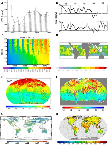
Fig. 13 Earth’s CO₂ history for (A) Precambrian, (B) Phanerozoic, (C) Quaternary, (D) late Quaternary, (E) Holocene, (F) Common Era, (G) 1880–2019, and (H) 2010 (continuous 5-minute data from towers).

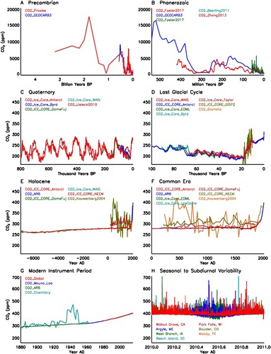
The modern instrument measurements of atmospheric CO₂ began in the early nineteenth century. The existence of CO₂ in Earth’s atmosphere was discovered by Joseph Black in 1752–1754 (Black, 1807; see review by Letts & Blake, 1902). Thenard (1813) devised the first method for measuring the atmospheric CO₂ concentration, while Pettenkofer (1858) designed a more accurate method. Numerous measurements have been conducted in the 140 years between 1812 and 1958 (e.g. Bischof, 1960; Brown & Escombe, 1905; Fonselius & Koroleff, 1955; Stanhill, 1982; see reviews by Letts & Blake, 1902 and Beck, 2007). For example, Stanhill (1982) presented a 33-year (1877–1910) time series of CO₂ concentrations measured at the Montsouris Observatory in France (Fig. 12A). Kreutz (1941) reported more than 64,000 measurements at the meteorological station in Giessen, Germany, between 1939 and 1941. Bischof (1960) presented 5 years (1955–1959) of continuous measurements from 19 stations in Scandinavia (Fig. 12B). Beck (2007) compiled data measured in rural areas from 180 papers and presented a 140-year (1812–1961) time series of CO₂ concentration. More works are needed to analyse and compile these historical CO₂ measurements, which may extend the current modern instrument time series back to the early nineteenth century. It would be interesting to conduct a side-by-side comparison of the old instruments and new instruments using the same air samples, and analyse the historical station locations together with nearby weather station data. Keeling (1958) invented a new technique for the measurement of atmospheric CO₂ using cryogenic condensation of air samples followed by NDIR spectroscopic analysis against a reference gas with manometric calibration. This technique was adopted for CO₂ determination throughout the world, including in the NOAA Global Greenhouse Gas Reference Network (e.g. Peters et al., 2007; Tans et al., 1989; Yuan et al., 2019). Measurements are also conducted on very high towers (Andrews et al., 2014; Bakwin et al., 1998; Miles et al., 2012) and aircrafts (Gerbig et al., 2003; Sweeney et al., 2015). A compilation of global in situ measurements since 1957 has been released by the Cooperative Global Atmospheric Data Integration Project (2017). In the past 60 years, the annual mean CO₂ concentration at Mauna Loa increased from 316 ppm in 1959 to 414 ppm in 2020. The year-to-year increasing rate is affected by ENSO (Bacastow, 1976; Bacastow et al., 1980; Betts et al., 2018; Jones et al., 2001; Keeling et al., 1995; Luo et al., 2018; Piao et al., 2020). Jones et al. (2001) showed that the CO₂ difference between El Nino and La Nina is about 0.5–2 ppm. Using a global terrestrial biosphere model, Betts et al. (2018) successfully predicted the record CO₂ rise associated with the 2015/2016 El Nino, which is mainly due to the weakening of tropical land carbon sink. For the annual cycle, Keeling et al. (1976) reported a range of 6 ppm at Mauna Loa, Yuan et al. (2019) reported a range of 10 ppm at Mount Zugspitze, Germany, while the global marine surface average shows a range of 4 ppm. The range of annual cycle is much stronger in the northern hemisphere than in the southern hemisphere (Jiang et al., 2016; Fig. 12C). Using tower measurements across the United States, Bakwin et al. (1998) found that the range of annual cycle increases with a height from 10 ppm at the surface to ∼30 ppm above 100 m height. For the diurnal cycle, Yuan et al. (2019) reported a range of 1 ppm at Mauna Loa and 1–2 ppm at Mount Zugspitze, Germany. Bakwin et al. (1998) found that the range of diurnal cycle in the central U.S. decreases significantly with height in summer from >40 ppm at 10 m to <5 ppm above 400 m.

Satellite measurements of atmospheric CO₂ have been conducted using different sensors such as the High-Resolution Infrared Radiation Sounder (HIRS) onboard the NOAA polar orbiting satellites (Chedin et al., 2003), the Infrared Atmospheric Sounding Interferometer (IASI) onboard the European MetOp satellite (Crevoisier et al., 2009; Fig. 12D), the Atmospheric Infrared Sounder (AIRS) instrument onboard NASA’s AQUA satellite (Crevoisier et al., 2004; Chahine et al., 2008; Pagano et al., 2014; Fig. 12E), the Orbiting Carbon Observatory-2 (OCO-2) (Eldering et al., 2017a, 2017b; Fig. 12F), the Greenhouse Gases Observing Satellite (GOSAT) (Crisp et al., 2012; Hammerling et al., 2012; Yokota et al., 2009; Fig. 12G), and the SCanning Imaging Absoprtion spectroMeter for Atmospheric CHartographY (SCIAMACHY) instrument onboard the ENVISAT satellite (Buchwitz et al., 2005; Schneising et al., 2011; Fig. 12H). All satellite maps show strong spatial variability of CO₂ concentration. In the tropics, the seasonal mean CO₂ concentration demonstrates a 10-ppm difference between different locations (Fig. 12D). Over the globe, the climatological monthly mean CO₂ concentration shows a 10-ppm difference between the Arctic and the southern oceans (Fig. 12C, E). High-resolution monthly satellite maps over the continents show larger spatial variability (Fig. 12F, G). The annual mean map still shows a strong spatial variability with ∼10-ppm differences among different regions (Fig. 12H). The strong spatial variability may explain the difference between Antarctic ice core data and Greenland ice core data, the difference between Antarctic ice core and other proxies such as the stomata, and the difference between the chemistry measurements in 1812–1958 and later measurements (Fig. 11E–H, Fig. 12A–B).

CO₂ concentration demonstrates the most dramatic variability among the different components of Earth’s climate system (Fig. 13). Precambrian CO₂ concentration reaches 17,000 ppm around 2 billion years BP, which is 50 times today’s value (Fig. 13A). Phanerozoic CO₂ concentration oscillates by 4000–10,000 ppm (Fig. 13B). The oscillation amplitude decreases significantly to 60–100 ppm for Quaternary interglacial cycles (Fig. 13C) and 10–20 ppm for Heinrich and D–O events in the last glacial cycle (Fig. 13D). For Holocene and Common Era, the Greenland ice cores report higher CO₂ concentrations than the Antarctica ice cores, while the stomata reconstructions show larger variabilities than the ice core reconstructions (Fig. 13E–F). For the modern measurement period, the chemistry measurements before 1958 show larger variabilities than later measurements (Fig. 13G). Similar to temperature and sea level, CO₂ oscillation amplitudes increase substantially at seasonal and diurnal timescales. Fig. 13H illustrates the continuous 5-minute CO₂ measurements from towers at different latitudes, which are generally considered the most accurate measurements of CO₂ concentration. CO₂ concentrations oscillate by about 200 ppm at a high-latitude inland station, 150 ppm at a high-latitude station near the coast, and 30–50 ppm at a subtropical station. These are contributed by the seasonal cycle, diurnal cycle, as well as other high-frequency variability.

6 Summary and discussions

This paper synthesized the first global unified picture of Earth’s climate history from the longest timescale to the current climate, which provides an observational benchmark for understanding and modelling Earth’s climate system and global climate change. Earth’s climate history shows dominant climate modes such as the supercontinent cycles, interglacial cycles, millennial cycles, multi-decadal oscillation, interannual oscillation, seasonal cycle and diurnal cycle. The amplitudes of the dominant climate variability generally decrease from the billion-year timescales to interannual timescales, then significantly increase at the seasonal to diurnal timescales (Fig. 14). For oscillations at each timescale, comparing the phase of temperature (Fig. 7), sea level (Fig. 10) and CO₂ (Fig. 13) can reveal important physical relationships and possible underlying mechanisms.

Fig. 14 Summary of the amplitudes of dominant climate variability. The amplitudes of oscillations are estimated using standard deviation multiplied by 2, while that of global warming is simply the increase from 1880 to 2020.

The Earth’s climate history is modulated by external forcings and internal feedbacks (Fig. 2). The external forcings change with time and can drive trends and oscillations. For example, theories suggest that solar luminosity was weak in Precambrian and had been increasing since then (Feulner, 2012). The solar forcing at 4 Ga was ∼75% of today’s value. On top of this multi-billion-year trend, there is rich variability generated by changes in Earth’s orbit and the planetary system, such as the Milankovitch cycles dominating the Quaternary climate. The internal feedbacks also change with time. For example, the ocean-atmosphere feedback is dominated by upper ocean processes for the interannual ENSO (Bjerknes, 1969) but by deep ocean thermohaline circulation for the multi-decadal AMO and millennial Heinrich/D–O/Bond events (Lynch-Stieglitz, 2017; Zhang et al., 2019), deep ocean halothermal circulation for the Phanerozoic climate (Hay, 2008; Horne, 1999), and entire ocean mixing for the Precambrian climate events (Ashkenazy et al., 2013; Hoffman et al., 2017). The interplay of the external forcings and internal feedbacks led to the observed Earth’s climate history.

The physical processes connecting Earth’s surface temperature, sea level and CO₂ are complicated and vary at different timescales, which are under active research. A highly simplified framework assumes that variations of CO₂ controls variations of Earth’s surface temperature, while other physical processes provide feedbacks to either enhance or reduce the resultant temperature change. Following this framework, an equilibrium climate sensitivity is often defined as the steady-state global surface temperature increase for a doubling of CO₂ (IPCC, 2007; IPCC, 2013; IPCC, 2021; Sherwood et al., 2020), which has been accessed using observational datasets from modern instrument period (e.g. Gregory et al., 2002; Lewis & Curry, 2015, 2018; Skeie et al., 2014), the Common Era (Hegerl et al., 2006; Rind et al., 2004), the last glacial cycle (e.g. Annan & Hargreaves, 2013; Schmittner et al., 2011), the late Quaternary (e.g. Köhler et al., 2015, 2017; Royer, 2016; Snyder, 2019), the Cenozoic (e.g. Hansen et al., 2013; Inglis et al., 2020; PALAEOSENS, 2012; Rae et al., 2021; Zhu et al., 2020) and the Phanerozoic (e.g. Farnsworth et al., 2019). The estimated equilibrium climate sensitivity varies significantly at different timescales. This is likely because the highly simplified framework of CO₂ controlling temperature may not be valid when other physical processes unrelated to CO₂, such as solar forcing and plate tectonics, are playing a key or leading role in changing Earth’s temperature. Similarly, sea level is affected not only by temperature but also by plate tectonics (sea area, dynamic topography, ridge volume, sea floor volcanism, icesheet-induced isostatic depression) and ocean sediment thickness, which dominate sea-level change at timescales longer than one million years (Fig. 8A, B).

There are numerous unanswered questions about Earth’s climate history. For the Precambrian climate, there are three key unanswered questions. The first one is a long-lasting question of how the Earth kept a warm temperature when the solar forcing was ∼70% of today’s value, which is termed the “faint young sun problem” (Feulner, 2012; Hu & Tian, 2015). All temperature reconstructions show anomalies of 20–60°C warmer than today’s temperature (Fig. 7A), which is difficult to explain using the observed CO₂ concentrations (Fig. 13A). The second question is the “snowball Earth” hypothesis (Hoffman et al., 2017; Kirschvink, 1992), which is based on the observations of widespread low-latitude glaciation in both Palaeoproterozoic era (Evans et al., 1997) and Neoproterozoic era (Hoffman et al., 1998). However, none of the temperature reconstructions show a temperature anomaly significantly colder than today’s temperature (Fig. 7A). Higher-resolution datasets are needed to resolve any possible short-term events. The third question is how climate changes are associated with the supercontinent cycles. Theories suggest that the assembly of the supercontinent tends to cause a decrease in sea level, a decrease in CO₂ concentration, and a cooling of Earth’s surface temperature. The latest temperature (Fig. 7A) and sea level (Fig. 10A) curves appear to support the theories, while the number of CO₂ observations is not enough to resolve any changes associated with the supercontinent cycles (Fig. 13A). More efforts are needed to collect new datasets and develop new methods and new proxies.

For the Phanerozoic climate, an interesting question is why temperature (Fig. 7B) does not show a double-hump curve similar to sea level (Fig. 10B) and CO₂ (Fig. 13B)? The temperature curves, on the other hand, are dominated by higher-frequency oscillations. Theories suggest that the higher-frequency oscillations are mainly driven by external solar forcing rather than the greenhouse effect or ice-sheet dynamics.

For the interglacial cycles, the ocean temperature (Fig. 7C), sea level (Fig. 10C) and CO₂ (Fig. 13C) are all dominated by the 100-ka eccentricity cycle, while the continental temperature is often dominated by the 41-ka obliquity cycle. There are three key unanswered questions. First, why is ocean temperature dominated by the 100-ka eccentricity cycle when the solar insolation is dominated by the 41-ka obliquity cycle and 23-ka precession cycle? This is the long-lasting “100,000-yr problem” (Lisiecki, 2010). Secondly, why did the dominant oscillation period change from 100- to 41-ka before 1 Ma? Thirdly, most of the Quaternary datasets are orbitally tuned, making it difficult to examine the phase relationship among different regions or among temperature, sea level and CO₂. How can we develop accurate un-tuned Quaternary datasets?

The climate of the last glacial cycle is dominated by millennial-scale variability, especially the Heinrich events and D–O events. These events generate strong surface temperature signals around the world (Fig. 7D), as well as significant sea-level signals (Fig. 10D) and CO₂ signals (Fig. 13D). It is well established that the Heinrich events and D–O events are closely connected to the Atlantic Meridional Overturning Circulation (AMOC). However, observations show that the fresh water input lags the abrupt climate transitions, and model experiments of AMOC changes show overly weak global responses compared to observations. There are two key unanswered questions. First, what drive the AMOC transitions associated with the Heinrich and D–O events? Secondly, what drive the observed strong global signals associated with the Heinrich and D–O events?

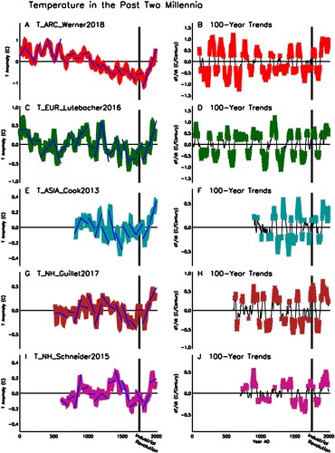
The Holocene and Common Era are the time periods with the largest number of observational data (Fig. 5C–D). Palaeoclimate field reconstructions and palaeoclimate reanalysis have been developed using these datasets. There are three key questions. The first important question is how to combine datasets with different dating methods since annual layer counting has high accuracy, but radiometric dating has large uncertainty at these timescales. The standard deviation of radiometric ages could be 40–150 years. Synchronization of nearby records, such as what the GICC2005 chronology did for the Greenland ice cores (Andersen et al., 2006; Rasmussen et al., 2006; Svensson et al., 2006; Vinther et al., 2006), would significantly improve the dating. The second question is whether the Bond events are global events and whether the little ice age is part of the Bond cycles. The third question is whether the ongoing global warming is unprecedented in the Common Era or the Holocene. Fig. 15 shows the regional mean surface temperature in the past 2000 years for (A) Arctic (Werner et al., 2018), (C) Europe (Lutebacher et al., 2016), (E) Asia (Cook et al., 2013), (G) Northern Hemisphere (Guillet et al., 2017), and (I) Northern Hemisphere (Schneider et al., 2015). Linear trends are shown for 100-year periods ending at 100AD, 200AD, … , 1900AD and the last year of data (blue lines). The corresponding 100-year running trends (warming rates) are shown in (B) (D) (F) (H) and (J), respectively, which is defined as a linear trend of temperature for the 100-year period ending at the year of interest. Both the temperature records and the warming rates show significant oscillations. Warming rates before the industrial revolution are sometimes comparable to or even higher than the maximum warming rate in the industrial era. Therefore, in terms of the warming rate, the ongoing warmings of Arctic, Europe, Asia and Northern Hemisphere are not unprecedented in the past 2000 years. Larger uncertainties are associated with the reconstruction of global mean surface temperature.

Fig. 15 Regional mean surface temperature in the past 2000 years for (A) Arctic (Werner et al., 2018), (C) Europe (Lutebacher et al., 2016), (E) Asia (Cook et al., 2013), (G) Northern Hemisphere (Guillet et al., 2017), and (I) Northern Hemisphere (Schneider et al., 2015). Linear trends are shown for 100-year periods ending at 100AD, 200AD, … , 1900AD and last year of data (blue lines). The corresponding 100-year running trends (warming rates) are shown in (B) (D) (F) (H) and (J), respectively. Colour stars denote the linear trends that are above the 95% confidence level.

We are witnessing rapid advances in palaeoclimatology and expect to see the following progress in the near future:

1. New dating methods, especially un-tuned dating for interglacial cycles.

2. Synchronization and inter-calibration of nearby records.

3. Intercomparison of different proxies, especially for CO₂.

4. High-resolution reconstructions of Holocene climate.

5. Palaeoclimate reanalysis for Holocene, the last glacial cycle and Quaternary.

6. Collection of more datasets for Precambrian and Phanerozoic climate.

In the next 50 years, we might be able to finish the data collection and analysis for palaeoclimatology, develop Earth system models for all timescales, and achieve a comprehensive understanding of Earth’s climate history. The Earth’s four layers – atmosphere, hydrosphere, mantle and core – are all rotating and convecting fluids. Geophysical fluid dynamics was founded by Laplace, who published the famous Laplace equations of tidal dynamics in the late eighteenth century (Laplace, 1775, 1798). These are basically linearized forms of the primitive equations and have been used to this day in studying atmospheric and ocean tides. The Navier–Stokes equations were determined in the nineteenth century (Navier, 1822; Stokes, 1842). The complete primitive equations were published by Poincare (1901) and V. Bjerknes (1904), which were applied later to theoretical atmospheric models (e.g. J. Bjerknes, 1937; Rossby, 1939), ocean models (e.g. Ekman, 1905; Sverdrup, 1947), mantle models (e.g. Pekeris, 1935; Runcorn, 1962) and core geodynamo models (e.g. Herzenberg, 1958; Larmor, 1919). Using computers, numerical models have been developed for all four layers based on primitive equations. It would be possible to combine the models for the four layers to form a model of the whole Earth system, which will be able to simulate Earth’s climate variability from 4.5 billion years to one minute.

Acknowledgements

Part of this work was done by TQ when working in the Department of Geography, The Ohio State University. We thank Paul Knauth for sharing the Precambrian chert dataset and discussions on temperature estimates, Christian Verard for sharing the Phanerozoic sea level datasets, and Phil Woodsworth for his comments on an earlier version of the manuscript.

Disclosure statement

No potential conflict of interest was reported by the author(s).

Additional information

Funding

This study was supported by NSF Grant AGS-1347132.

References

- Ablain, M., Cazenave, A., Larnicol, G., Balmaseda, M., Cipollini, P., Faugère, Y., Fernandes, M. J., Henry, O., Johannessen, J. A., Knudsen, P., Andersen, O., Legeais, J., Meyssignac, B., Picot, N., Roca, M., Rudenko, S., Scharffenberg, M. G., Stammer, D., Timms, G., & Benveniste, J. (2015). Improved sea level record over the satellite altimetry era (1993–2010) from the climate change initiative project. Ocean Science, 11(1), 67–82. https://doi.org/10.5194/os-11-67-2015
- Abraham, K., Hofmann, A., Foley, S. F., Cardinal, D., Harris, C., Barth, M. G., & Andre, L. (2011). Coupled silicon-oxygen isotope fractionation traces Archaean silicification. Earth and Planetary Science Letters, 301(1–2), 222–230. https://doi.org/10.1016/j.epsl.2010.11.002
- Ackerson, M. R., Mysen, B. O., Tailby, N. D., & Watson, E. B. (2018). Low-temperature crystallization of granites and the implications for crustal magmatism. Nature, 559(7712), 94–97. https://doi.org/10.1038/s41586-018-0264-2
- Affolter, S., Hauselmann, A., Fleitmann, D., Edwards, R. L., Cheng, H., & Leuenberger, M. (2019). Central Europe temperature constrained by speleothem fluid inclusion water isotopes over the past 14,000 years. Science Advances, 5(6), eaav3809. https://doi.org/10.1126/sciadv.aav3809
- Ahn, J., & Brook, E. J. (2008). Atmospheric CO2 and climate on millennial time scales during the last glacial period. Science, 322(5868), 83–85. https://doi.org/10.1126/science.1160832
- Ahn, J., Brook, E. J., Mitchell, L., Rosen, J., McConnell, J. R., Taylor, K., Etheridge, D., & Rubino, M. (2012). Atmospheric CO2 over the last 1000 years: A high-resolution record from the West Antarctic Ice Sheet (WAIS) Divide ice core. Global Biogeochemical Cycles, 26, GB2027. https://doi.org/10.1029/2011GB004247
- Alley, R. B. (2000). The Younger Dryas cold interval as viewed from central Greenland. Quaternary Science Reviews, 19(1–5), 213–226. https://doi.org/10.1016/S0277-3791(99)00062-1
- Anchukaitis, K., & McKay, N. (2014). PAGES2k: Advances in Climate Field Reconstructions. PAGES Magazine, 22, 98.
- Andersen, K. K., Svensson, A., Rasmussen, S. O., Steffensen, J. P., Johnsen, S. J., Bigler, M., Röthlisberger, R., Ruth, U., Siggaard- Andersen, M.-L., Dahl-Jensen, D., Vinther, B. M., & Clausen, H. B. (2006). The Greenland Ice Core Chronology 2005, 15–42 ka. Part 1: Constructing the time scale. Quaternary Science Review, 25(23-24), 3246–3257. https://doi.org/10.1016/j.quascirev.2006.08.002
- Andre, L., Cardinal, D., Alleman, L. Y., & Moorbath, S. (2006). Silicon isotopes in 3.8 Ga West Greenland rocks as clues to the Eoarchaean supracrustal Si cycle. Earth and Planetary Science Letters, 245(1–2), 162–173. https://doi.org/10.1016/j.epsl.2006.02.046
- Andrews, A. E., Kofler, J. D., Trudeau, M. E., Williams, J. C., Neff, D. H., Masarie, K. A., Chao, D. Y., Kitzis, D. R., Novelli, P. C., Zhao, C. L., Dlugokencky, E. J., Lang, P. M., Crotwell, M. J., Fischer, M. L., Parker, M. J., Lee, J. T., Baumann, D. D., Desai, A. R., Stanier, C. O., … Tans, P. P. (2014). CO2, CO, and CH4 measurements from tall towers in the NOAA Earth System Research Laboratory’s Global Greenhouse Gas Reference Network: Instrumentation, uncertainty analysis, and recommendations for future high-accuracy greenhouse gas monitoring efforts. Atmospheric Measurement Techniques, 7(2), 647–687. https://doi.org/10.5194/amt-7-647-2014
- Angulo, R. J., & Lessa, G. C. (1997). The Brazilian sea-level curves: A critical review with emphasis on the curves from the Paranagua and Cananeia regions. Marine Geology, 140(1–2), 141–166. https://doi.org/10.1016/S0025-3227(97)00015-7
- Angulo, R. J., Lessa, G. C., & de Souza, M. C. (2005). A critical review of mid- to late-Holocene sea-level fluctuations on the eastern Brazilian coastline. Quaternary Science Review, 25(5–6), 486–506. https://doi.org/10.1016/j.quascirev.2005.03.008
- Anklin, M., Barnola, J.-M., Schwander, J., Stauffer, B., & Raynaud, D. (1995). Processes affecting the CO2 concentrations measured in Greenland ice. Tellus, J7B(4), 461–470. https://doi.org/10.1034/j.1600-0889.47.issue4.6.x
- Anklin, M., Schwander, J., Stauffer, B., Tschumi, J., Fuchs, A., Barnola, J.-M., & Raynaud, D. (1997). CO2 record between 40 and 8 kyr B.P. from the GRIP ice core. Journal of Geophysical Research, 102(C12), 26539–26545. https://doi.org/10.1029/97JC00182
- Annan, J. D., & Hargreaves, J. C. (2013). A new global reconstruction of temperature changes at the Last Glacial Maximum. Climate of the Past, 9(1), 367–376. https://doi.org/10.5194/cp-9-367-2013
- Arrhenius, G., Kjellberg, G., & Libby, W. F. (1951). Age determination of Pacific chalk ooze by radiocarbon and titanium content. Tellus, 3(4), 222–229. https://doi.org/10.3402/tellusa.v3i4.8662
- Arz, H. W., Lamy, F., Ganopolski, A., Novaczyk, N., & Patzold, J. (2007). Dominant northern hemisphere climate control over millennial-scale sea-level variability. Quaternary Science Reviews, 26(3–4), 312–321. https://doi.org/10.1016/j.quascirev.2006.07.016
- Ashkenazy, Y., Gildor, H., Losch, M., Macdonald, F. A., Schrag, D. P., & Tziperman, E. (2013). Dynamics of a Snowball Earth ocean. Nature, 495(7439), 90–93. https://doi.org/10.1038/nature11894
- Asmerom, Y., Polyak, V., Burns, S., & Rassmussen, J. (2007). Solar forcing of Holocene climate: New insights from a speleothem record, southwestern United States. Geology, 35(1), 1–4. https://doi.org/10.1130/G22865A.1
- Aston, F. W. (1919). A positive ray spectrograph. Philosophical Magazine, 38(228), 707–715. https://doi.org/10.1080/14786441208636004
- Bacastow, R. (1976). Modulation of atmospheric carbon dioxide by the Southern Oscillation. Nature, 261(5556), 116–118. https://doi.org/10.1038/261116a0
- Bacastow, R., Adams, J., Keeling, C., Moss, D., Whorf, T., & Wong, C. (1980). Atmospheric carbon dioxide, the southern oscillation, and the weak 1975 El Nino. Science, 210(4465), 66–68. https://doi.org/10.1126/science.210.4465.66
- Bajolle, L., Larocque-Tobler, I., Gandouin, E., Lavoie, M., Bergeron, Y., & Ali, A. (2018). Major postglacial summer temperature changes in the central coniferous boreal forest of Quebec (Canada) inferred using chironomid assemblages. Journal of Quaternary Science, 33(4), 409–420. https://doi.org/10.1002/jqs.3022
- Bakwin, P. S., Tans, P. P., Hurst, D. F., & Zhao, C. L. (1998). Measurements of carbon dioxide on very tall towers: Results of the NOAA/CMDL program. Tellus B-Chemical and Physical Meteorology, 50(5), 401–415. https://doi.org/10.3402/tellusb.v50i5.16216
- Banjeree, P. K. (2000). Holocene and late Pleistocene relative sea level fluctuations along the east coast of India. Marine Geology, 167(3–4), 243–260. https://doi.org/10.1016/S0025-3227(00)00028-1
- Bar-Matthews, M., Ayalon, A., Gilmour, M., Matthews, A., & Hawkesworth, C. J. (2003). Sea-land oxygen isotopic relationships from planktonic foraminifera and speleothems in the Eastern Mediterranean region and their implication for paleorainfall during interglacial intervals. Geochimica et Cosmochimica Acta, 67(17), 3181–3199. https://doi.org/10.1016/S0016-7037(02)01031-1
- Bard, E. (2002). Climate shock: Abrupt climate changes over millennial time scales. Physics Today, 55(12), 32–38. https://doi.org/10.1063/1.1537910
- Bard, E., Hamelin, B., & Fairbanks, R. G. (1990). U-Th ages obtained by mass spectrometry in corals from Barbados: Sea level during the past 130000 years. Nature, 346(6283), 456–458. https://doi.org/10.1038/346456a0
- Barnola, J. M., Anklin, M., Porcheron, J., Raynaud, D., Schwander, J., & Stauffer, B. (1995). CO2 evolution during the last millennium as recorded by Antarctic and Greenland ice. Tellus B: Chemical and Physical Meteorology, 47(1–2), 264–272. https://doi.org/10.3402/tellusb.v47i1-2.16046
- Barnola, J. M., Raynaud, D., Korotkevich, Y. S., & Lorius, C. (1987). Vostok ice cores provides 160,000-year record of atmospheric CO2. Nature, 329(6138), 408–414. https://doi.org/10.1038/329408a0
- Barnola, J., Raynaud, D., Neftel, A., & Oeschger, H. (1983). Comparison of CO2 measurements by two laboratories on air from bubbles in polar ice. Nature, 303(5916), 410. https://doi.org/10.1038/303410a0
- Barron, J. A., Heusser, L., Herbert, T., & Lyle, M. (2003). High resolution climatic evolution of coastal northern California during the past 16,000 years. Paleoceanography, 18(1), 1020. https://doi.org/10.1029/2002PA000768
- Bauska, T. K., Marcott, S. A., & Brook, E. J. (2021). Abrupt changes in the global carbon cycle during the last glacial period. Nature Geoscience, 14(2), 91–96. https://doi.org/10.1038/s41561-020-00680-2
- Bazin, L., Landais, A., Lemieux-Dudon, B., Toyé Mahamadou Kele, H., Veres, D., Parrenin, F., Martinerie, P., Ritz, C., Capron, E., Lipenkov, V., Loutre, M.-F., Raynaud, D., Vinther, B., Svensson, A., Rasmussen, S. O., Severi, M., Blunier, T., Leuenberger, M., Fischer, H., Masson-Delmotte, V., Chappellaz, J., & Wolff, E. (2013). An optimized multi-proxy, multi-site Antarctic ice and gas orbital chronology (AICC2012): 120–800 ka. Climate of the Past, 9(4), 1715–1731. https://doi.org/10.5194/cp-9-1715-2013
- Beck, E. G. (2007). 180 years of atmospheric CO2 gas analysis by chemical methods. Energy & Environment, 18(2), 259–282. https://doi.org/10.1177/0958305X0701800206
- Beerling, D. J., & Royer, D. L. (2011). Convergent Cenozoic CO2 history. Nature Geoscience, 4(7), 418–420. https://doi.org/10.1038/ngeo1186
- Bemis, B. E., & Spero, H. J. (1998). Reevaluation of the oxygen isotopic composition of planktonic foraminifera: Experimental results and revised paleotemperature equations. Paleoceanography, 13(2), 150–160. https://doi.org/10.1029/98PA00070
- Bennike, O., Wagner, B., & Richter, A. (2011). Relative sea level changes during the Holocene in the Sisimiut area, south-western Greenland. Journal of Quaternary Science, 26(4), 353–361. https://doi.org/10.1002/jqs.1458
- Bereiter, B., Eggleston, S., Schmitt, J., Nehrbass-Ahles, C., Stocker, T. F., Fischer, H., Kipfstuhl, S., & Chappellaz, J. (2015). Revision of the EPICA Dome C CO2 record from 800 to 600 kyr before present. Geophysical Research Letters, 42(2), 542–549. https://doi.org/10.1002/2014GL061957
- Bereiter, B., Lüthi, D., Siegrist, M., Schüpbach, S., Stocker, T. F., & Fischer, H. (2012). Mode change of millennial CO2 variability during the last glacial cycle associated with a bipolar marine carbon seesaw. Proceedings of the National Academy of Sciences, 109(25), 9755–9760. https://doi.org/10.1073/pnas.1204069109
- Berner, R. A. (1991). A model for atmospheric CO2 over Phanerozoic time. American Journal of Science, 291(4), 339–376. https://doi.org/10.2475/ajs.291.4.339
- Berner, R. A. (1994). GEOCARB II: A revised model of atmospheric CO2 over Phanerozoic time. American Journal of Science, 294(1), 56–91. https://doi.org/10.2475/ajs.294.1.56
- Berner, R. A. (2006). GEOCARBSULF: A combined model for Phanerozoic atmospheric O2 and CO2. Geochimica et Cosmochimica Acta, 70(23), 5653–5664. https://doi.org/10.1016/j.gca.2005.11.032
- Berner, R. A., & Kothavala, Z. (2001). GEOCARB III: A revised model of atmospheric CO2 over Phanerozoic time. American Journal of Science, 301(2), 182–204. https://doi.org/10.2475/ajs.301.2.182
- Betts, H. C., Puttick, M. N., Clark, J. W., Williams, T. A., Donoghue, P. C. J., & Pisani, D. (2018). Integrated genomic and fossil evidence illuminates life’s early evolution and eukaryote origin. Nature Ecology and Evolution, 2, 1556–1562. https://doi.org/10.1038/s41559-018-0644-x
- Bintanja, R., Roderik, S. W., & van de Wal, O. J. (2005). Modeled atmospheric temperatures and global sea levels over the past million years. Nature, 437(7055), 125–128. https://doi.org/10.1038/nature03975
- Bird, B. W., Abbott, M. B., Rodbell, D. T., & Vuille, M. (2011). Holocene tropical South American hydroclimate revealed from a decadally resolved lake sediment δ18O record. Earth and Planetary Science Letters, 310(3–4), 192–202. https://doi.org/10.1016/j.epsl.2011.08.040
- Bischof, W. (1960). Periodical variations of the atmospheric CO, content in Scandinavia. Tellus, 12(2), 216–226. https://doi.org/10.1111/j.2153-3490.1960.tb01303.x
- Bjerknes, J. (1937). Die Theorie der aussertropischen Zyklonenbildung. Meteorologische Zeitschrift, 54, 460–466.
- Bjerknes, J. (1969). Atmospheric teleconnections from the equatorial Pacific. Monthly Weather Review, 97(3), 163–172. https://doi.org/10.1175/1520-0493(1969)097%3C0163:ATFTEP%3E2.3.CO;2
- Bjerknes, V. (1904). Das Problem der Wettervorhersage, betrachtet vom Standpunkte der Mechanik und der Physik. Meteorologische Zeitschrift, 21, 1–7.
- Black, J. (1807). Lectures on the elements of chemistry delivered in the University of Edinburgh. Mathew Carey.
- Blake, R. E., Chang, S. J., & Lepland, A. (2010). Phosphate oxygen isotope evidence for a temperate and biologically active Archean ocean. Nature, 464(7291), 1029–1032. https://doi.org/10.1038/nature08952
- Bond, G. C., Kromer, B., Beer, J., Muscheler, R., Evans, M. N., Showers, W., Hoffmann, S., Lotti-Bond, R., Hajdas, I., & Bonani, G. (2001). Persistent solar influence on North Atlantic climate during the Holocene. Science, 294(5549), 2130–2136. https://doi.org/10.1126/science.1065680
- Bond, G. C., Showers, W., Elliot, M., Evans, M., Lotti, R., Hajdas, I., Bonani, G., & Johnsen, S. (1999). The North Atlantic’s 1–2 kyr climate rhythm: Relation to Heinrich events, Dansgaard/Oeschger cycles and the little ice age. In P. U. Clark, R. S. Webb, & L. D. Keigwin (Eds.), Mechanisms of global climate change at millennial time scales (Geophysical Monograph Series, Vol. 112, pp. 35–68). https://agupubs.onlinelibrary.wiley.com/doi/book/10. 1029/GM112
- Bony, S., & Dufresne, J.-L. (2005). Marine boundary layer clouds at the heart of cloud feedback uncertainties in climate models. Geophysical Research Letters, 32(20), L20806. https://doi.org/10.1029/2005GL023851
- Briffa, K. R. (2000). Annual climate variability in the Holocene: Interpreting the message of ancient trees. Quaternary Science Reviews, 19(1–5), 87–105. https://doi.org/10.1016/S0277-3791(99)00056-6
- Broecker, W. S., Olson, E. A., & Orr, P. C. (1960). Radiocarbon measurement and annual rings in cave formations. Nature, 185, 93–94. https://doi.org/10.1038/185093a0
- Brooks, C. E. P. (1928). The influence of forests on rainfall and run-off. Quarterly Journal of the Royal Meteorological Society, 54(225), 1–17. https://doi.org/10.1002/qj.49705422501
- Brown, H., & Escombe, F. (1905). On the variation in the amount of carbon dioxide in the air of Kew during the years 1898–1901. Proceedings of the Royal Society B, 76, 118–121. https://doi.org/10.1098/rspb.1905.0004
- Buchwitz, M., de Beek, R., Burrows, J. P., Bovensmann, H., Warneke, T., Notholt, J., Meirink, J. F., Goede, A. P. H., Bergamaschi, P., Korner, S., Heimann, M., & Schulz, A. (2005). Atmospheric methane and carbon dioxide from SCIAMACHY satellite data: Initial comparison with chemistry and transport models. Atmospheric Chemistry and Physics, 5(4), 941–962. https://doi.org/10.5194/acp-5-941-2005
- Buizert, C., Cuffey, K. M., Severinghaus, J. P., Baggenstos, D., Fudge, T. J., Steig, E. J., Markle, B. R., Winstrup, M., Rhodes, R. H., Brook, E. J., Sowers, T. A., Clow, G. D., Cheng, H., Edwards, R. L., Sigl, M., McConnell, J. R., & Taylor, K. C. (2015). The WAIS Divide deep ice core WD2014 chronology – Part 1: Methane synchronization (68–31 ka BP) and the gas age-ice age difference. Climate of the Past, 11(2), 153–173. https://doi.org/10.5194/cp-11-153-2015
- Byers, H. R., & Braham, R. R. (1948). Thunderstorm circulation and structure. Journal of Meteorology, 5(3), 71–86. https://doi.org/10.1175/1520-0469(1948)005%3C0071:TSAC%3E2.0.CO;2
- Cacho, I., Grimalt, J. O., Pelejero, C., Canals, M., Sierro, F. J., Flores, J. A., & Shackleton, N. (1999). Dansgaard-Oeschger and Heinrich event imprints in Alboran Sea paleotemperatures. Paleoceanography, 14(6), 698–705. https://doi.org/10.1029/1999PA900044
- Camuera, J., Jimenez-Moreno, G., Ramos-Roman, M. J., Garcia-Alix, A., Toney, J. L., Anderson, R. S., Jimenez-Espejo, F., Bright, J., Webster, C., Yanes, Y., & Carrion, J. S. (2019). Vegetation and climate changes during the last two glacial-interglacial cycles in the western Mediterranean: A new long pollen record from Padul (southern Iberian Peninsula). Quaternary Science Review, 205, 86–105. https://doi.org/10.1016/j.quascirev.2018.12.013
- Carolin, S. A., Cobb, K. M., Adkins, J. F., Clark, B., Conroy, J. L., Lejau, S., Malang, J., & Tuen, A. A. (2013). Varied response of western Pacific hydrology to climate forcings over the last glacial period. Science, 340(6140), 1564–1566. https://doi.org/10.1126/science.1233797
- Castellani, B. B., Shupe, M. D., Hudak, D. R., & Sheppard, B. E. (2015). The annual cycle of snowfall at Summit, Greenland. Journal of Geophysical Research, 120(13), 6654–6668. https://doi.org/10.1002/2015JD023072
- Catling, D. C., & Zahnle, K. J. (2020). The Archean atmosphere. Science Advance, 6, eaax1420. https://doi.org/10.1126/sciadv.aax1420
- Chahine, M., Chen, L., Dimotakis, P., Jiang, X., Li, Q., Olsen, E. T., Pagano, T., Randerson, J., & Yung, Y. L. (2008). Satellite remote sounding of mid-tropospheric CO2. Geophysical Research Letters, 35(17), L17807. https://doi.org/10.1029/2008GL035022
- Chakrabarti, R., Knoll, A. H., Jacobsen, S. B., & Fischer, W. W. (2012). Si isotopic variability of Proterozoic cherts. Geochimica et Cosmochimica Acta, 91, 187–201. https://doi.org/10.1016/j.gca.2012.05.025
- Chappell, J., Omura, A., Ezat, T., McCulloch, M., Pandolfi, J., Ota, Y., & Pillans, B. (1996). Reconciliation of late Quaternary sea levels derived from coral terraces at Huon Peninsula with deep-sea oxygen isotope records. Earth and Planetary Science Letters, 141(1–4), 227–236. https://doi.org/10.1016/0012-821X(96)00062-3
- Chappell, J., & Shackleton, N. J. (1986). Oxygen isotopes and sea level. Nature, 324(6093), 137–140. https://doi.org/10.1038/324137a0
- Chedin, A., Serrar, S., Scott, N. A., Crevoisier, C., & Armante, R. (2003). First global measurement of midtropospheric CO2 from NOAA polar satellites: Tropical zone. Journal of Geophysical Research, 108(D18), 4581. https://doi.org/10.1029/2003JD003439
- Cheng, H., Edwards, L., Sinha, A., Spötl, C., Yi, L., Chen, S., Kelly, M., Kathayat, G., Wang, X. F., Li, X. L., Kong, X. G., Wang, Y. J., Ning, Y. F., & Zhang, H. W. (2016). The Asian monsoon over the past 640,000 years and ice age terminations. Nature, 534(7609), 640–646. https://doi.org/10.1038/nature18591
- Cheng, H., Springer, G. S., Sinha, A., Hardt, B. F., Yi, L., Li, H., Tian, Y., Li, X., Rowe, H. D., Kathayat, G., Ning, Y., & Edwards, R. L. (2019). Eastern North American climate in phase with fall insolation throughout the last three glacial-interglacial cycles. Earth and Planetary Science Letters, 522, 125–134. https://doi.org/10.1016/j.epsl.2019.06.029
- Church, J. A., & White, N. J. (2011). Sea-level rise from the late 19th to the early 21st century. Surveys in Geophysics, 32(4–5), 585–602. https://doi.org/10.1007/s10712-011-9119-1
- Ciais, P., Dolman, A. J., Bombelli, A., Duren, R., Peregon, A., Rayner, P. J., Miller, C., Gobron, N., Kinderman, G., Marland, G., Gruber, N., Chevallier, F., Andres, R. J., Balsamo, G., Bopp, L., Bréon, F.--M., Broquet, G., Dargaville, R., Battin, T. J., Borges, A., Bovensmann, H., Buchwitz, M., Butler, J., Canadell, J. G., Cook, R. B., DeFries, R., Engelen, R., Gurney, K. R., Heinze, C., Heimann, M., Held, A., Henry, M., Law, B., Luyssaert, S., Miller, J., Moriyama, T., Moulin, C., Myneni, R. B., Nussli, C., Obersteiner, M., Ojima, D., Pan, Y., Paris, J.-D., Piao, S. L., Poulter, B., Plummer, S., Quegan, S., Raymond, P., Reichstein, M., Rivier, L., Sabine, C., Schimel, D., Tarasova, O., Valentini, R., Wang, R., van der Werf, G., Wickland, D., Williams, M., & Zehner, C. (2014). Current systematic carbon-cycle observations and the need for implementing a policy-relevant carbon observing system. Biogeosciences, 11(13), 3547–3602. https://doi.org/10.5194/bg-11-3547-2014
- Clegg, B. F., Kelly, R., Clarke, G. H., Walker, I. R., & Hu, F. S. (2011). Nonlinear response of summer temperature to Holocene insolation forcing in Alaska. Proceedings of National Academy of Sciences, 108(48), 19299–19304. https://doi.org/10.1073/pnas.1110913108
- Clemens, S., Holbourn, A., Kubota, Y., Lee, K., Liu, Z., Chen, G., Nelson, A., & Fox-Kemper, B. (2018). Precession-band variance missing from East Asian monsoon runoff. Nature Communications, 9(1), 3364. https://doi.org/10.1038/s41467-018-05814-0
- Coachman, L. K., Hemmingson, E., & Scholader, P. F. (1958). Gases in glaciers. Science, 127(3309), 1288–1289. DOI: 10.1126/science.127.3309.1288
- Comas-Bru, L., Rehfeld, K., Roesch, C., Amirnezhad-Mozhdehi, S., Harrison, S. P., Atsawawaranunt, K., Ahmad, S. M., Brahim, Y. A., Baker, A., Bosomworth, M., Breitenbach, S. F. M., Burstyn, Y., Columbu, A., Deininger, M., Demény, A., Dixon, B., Fohlmeister, J., Hatvani, I. G., Hu, J., Kaushal, N., Kern, Z., Labuhn, I., Lechleitner, F. A., Lorrey, A., Martrat, B., Novello, V. F., Oster, J., Pérez-Mejías, C., Scholz, D., Scroxton, N., Sinha, N., Ward, B. M., Warken, S., Zhang, H., & SISAL Working Group members. (2020). SISALv2: A comprehensive speleothem isotope database with multiple age-depth models. Earth System Science Data, 12(4), 2579–2606. https://doi.org/10.5194/essd-12-2579-2020
- Conrad, C. P. (2013). The solid Earth’s influence on sea level. GSA Bulletin, 125(7–8), 1027–1052. https://doi.org/10.1130/B30764.1
- Cook, E. R., & Jacoby, G. C. (1977). Tree-ring–drought relationships in the Hudson Valley, New York. Science, 198(4315), 399–401. DOI: 10.1126/science.198.4315.399
- Cook, E. R., Krusic, P. J., Anchukaitis, K. J., Buckley, B. M., Nakatsuka, T., & Sano, M. (2013). Tree-ring reconstructed summer temperature anomalies for temperate East Asia since 800 CE. Climate Dynamics, 41(11–12), 2957–2972. https://doi.org/10.1007/s00382-012-1611-x
- Cooper, J. A. G., Green, A. N., & Compton, J. S. (2018). Sea-level change in southern Africa since the last Glacial Maximum. Quaternary Science Reviews, 201, 303–318. https://doi.org/10.1016/j.quascirev.2018.10.013
- Cooperative Global Atmospheric Data Integration Project. (2017). Multi-laboratory compilation of atmospheric carbon dioxide data for the period 1957–2016; obspack_co2_1_GLOBALVIEWplus_v3.2_2017_11_02. NOAA Earth System Research Laboratory, Global Monitoring Division. https://doi.org/10.15138/G3704H
- Cramer, B. S., Toggweiler, J. R., Wright, J. D., Katz, M. E., & Miller, K. G. (2009). Ocean overturning since the late Cretaceous: Inferences from a new benthic foraminiferal isotope compilation. Paleoceanography, 24(4), PA4216. https://doi.org/10.1029/2008PA001683
- Crevoisier, C., Chedin, A., Matsueda, H., Machida, T., Armante, R., & Scott, N. A. (2009). First year of upper tropospheric integrated content of CO2 from IASI hyperspectral infrared observations. Atmospheric Chemistry and Physics, 9(14), 4797–4810. https://doi.org/10.5194/acp-9-4797-2009
- Crevoisier, C., Heilliette, S., Chedin, A., Serrar, S., Armante, R., & Scott, N. A. (2004). Midtropospheric CO2 concentration retrieval from AIRS observations in the tropics. Geophysical Research Letters, 31(17), L17106. https://doi.org/10.1029/2004GL020141
- Crisp, D., Fisher, B. M., O'Dell, C., Frankenberg, C., Basilio, R., Bösch, H., Brown, L. R., Castano, R., Connor, B., Deutscher, N. M., Eldering, A., Griffith, D., Gunson, M., Kuze, A., Mandrake, L., McDuffie, J., Messerschmidt, J., Miller, C. E., Morino, I., Natraj, V., Notholt, J., O'Brien, D., Oyafuso, F., Polonsky, I., Robinson, J., Salawitch, R., Sherlock, V., Smyth, M., Suto, H., Taylor, T., Thompson, D. R., Wennberg, P. O., Wunch, D., & Yung, Y. L. (2012). The ACOS XCO2 retrieval algorithm. Part 2: Global XCO2 data characterization. Atmospheric Measurement Techniques, 5(4), 687–707. https://doi.org/10.5194/amt-5-687-2012
- Cruz, F. W., Jr., Burns, S. J., Karmann, I., Sharp, W. D., Vuille, M., Cardoso, A. O., Ferrari, J. A., Silva Dias, P. L., & Viana, O., Jr. (2005). Insolation-driven changes in atmospheric circulation over the past 116,000 years in subtropical Brazil. Nature, 434(7029), 63–66. https://doi.org/10.1038/nature03365
- Cuffey, K. M., Clow, G. D., Alley, R. B., Stuiver, M., Waddington, E. D., & Saltus, R. W. (1995). Large Arctic temperature change at the glacial-Holocene transition. Science, 270(5235), 455–458. https://doi.org/10.1126/science.270.5235.455
- Dahl-Jensen, D., Mosegaard, K., Gundestrup, N., Clow, G. D., Johnsen, S. J., Hansen, A. W., & Balling, N. (1998). Past temperatures directly from the Greenland Ice Sheet. Science, 282(5387), 268–271. https://doi.org/10.1126/science.282.5387.268
- Dangendorf, S., Hay, C., Calafat, F. M., Marcos, M., Piecuch, C. G., Berk, K., & Jensen, J. (2019). Persistent acceleration in global sea-level rise since the 1960s. Nature Climate Change, 9(9), 705–710. https://doi.org/10.1038/s41558-019-0531-8
- Dansgaard, W. (1964). Stable isotopes in precipitation. Tellus, 16(4), 436–468. https://doi.org/10.3402/tellusa.v16i4.8993
- Dansgaard, W., Johnsen, S., Clausen, H., & Langway, C. C., Jr. (1971). Climatic record revealed by the Camp Century ice core. In K. K. Turekian (Ed.), The late Cenozoic glacial ages (pp. 37–56). Yale University Press.
- Dansgaard, W., Johnsen, S. J., Clausen, H. B., Dahljensen, D., Gundestrup, N. S., Hammer, C. U., Hvidberg, C. S., Steffensen, J. P., Sveinbjornsdottir, A. E., Jouzel, J., & Bond, G. (1993). Evidence for general instability of past climate from a 250-kyr ice-core record. Nature, 364(6434), 218–220. https://doi.org/10.1038/364218a0
- Dansgaard, W., Johnsen, S. J., Møller, J., & Langway, C. C. (1969). One Thousand Centuries of Climatic Record from Camp Century on the Greenland Ice Sheet. Science, 166(3903), 377–380. https://doi.org/10.1126/science.166.3903.377
- Davis, B. A. S., Brewer, S., Stevenson, A. C., & Guiot, J. (2003). The temperature of Europe during the Holocene reconstructed from pollen data. Quaternary Science Reviews, 22(15–17), 1701–1716. https://doi.org/10.1016/S0277-3791(03)00173-2
- de Boer, B., Lourens, L. J., & van de Wal, R. S. W. (2014). Persistent 400,000-year variability of Antarctic ice volume and the carboncycle is revealed throughout the Plio-Pleistocene. Nature Communications, 5(1), 2999. https://doi.org/10.1038/ncomms3999
- Delmas, R. J. (1993). A natural artefact in Greenland ice-core CO2 measurements. Tellus, 45B, 391–396. https://doi.org/10.1034/j.1600-0889.1993.t01-3-00006.x
- Delmas, R. J., Ascencio, J. M., & Legrand, M. (1980). Polar ice evidence that atmospheric CO2 29,000 BP was 50% of present. Nature, 284(5752), 155–157. https://doi.org/10.1038/284155a0
- DelSole, T., Tippett, M. K., & Shukla, J. (2011). A significant component of unforced multidecadal variability in the recent acceleration of global warming. Journal of Climate, 24(3), 909–926. https://doi.org/10.1175/2010JCLI3659.1
- Dempster, A. J. (1918). A new method of positive ray analysis. Physical Review, 11, 316–325. https://doi.org/10.1103/PhysRev.11.316
- Denniston, R. F., Asmerom, Y., Polyak, V. J., Wanamaker, A. D., Ummenhofer, C. C., Humphreys, W. F., Cugley, J., Woods, D., & Lucker, S. (2017). Decoupling of monsoon activity across the northern and southern Indo-Pacific during the late Glacial. Quaternary Science Reviews, 176, 101–105. https://doi.org/10.1016/j.quascirev.2017.09.014
- Ding, T., Gao, J., Tian, S., Fan, C., Zhao, Y., Wan, D., & Zhou, J. (2017). The δ30Si peak value discovered in middle Proterozoic chert and its implication for environmental variations in the ancient ocean. Scientific Report, 7(1), 44000. https://doi.org/10.1038/srep44000
- Dirmeyer, P. A., Cash, B. A., Kinter, J. L., III, Stan, C., Jung, T., Marx, L., Towers, P., Wedi, N., Adams, J. M., Altshuler, E. L., & Huang, B. (2012). Evidence for enhanced land-atmosphere feedback in a warming climate. Journal of Hydrometeorology, 13(3), 981–995. https://doi.org/10.1175/JHM-D-11-0104.1
- Ditlevsen, P., Mitsui, T., & Michel Crucifix, M. (2020). Crossover and peaks in the Pleistocene climate spectrum; understanding from simple ice age models. Climate Dynamics, 54(3–4), 1801–1818. https://doi.org/10.1007/s00382-019-05087-3
- Dodd, M. S., Papineau, D., Grenne, T., Slack, J. F., Rittner, M., Pirajno, F., O'Neil, J., & Little, C. T. (2017). Evidence for early life in Earth’s oldest hydrothermal vent precipitates. Nature, 543(7643), 60–64. https://doi.org/10.1038/nature21377
- Dorale, J. A., Edwards, R. L., Ito, E., & Gonzalez, L. A. (1998). Climate and vegetation history of the midcontinent from 75 to 25 ka: A speleothem record from Crevice Cave, Missouri, USA. Science, 282(5395), 1871–1874. https://doi.org/10.1126/science.282.5395.1871
- Douglass, A. E. (1909). Weather cycles in the growth of big trees. Monthly Weather Review, 37(6), 225–237. https://doi.org/10.1175/1520-0493(1909)37[225d:WCITGO]2.0.CO;2
- Driese, S. G., Jirsa, M. A., Ren, M., Brantley, S. L., Sheldon, N. D., Parker, D., & Schmitz, M. (2011). Neoarchean paleoweathering of tonalite and metabasalt: Implications for reconstructions of 2.69 Ga early terrestrial ecosystems and paleoatmospheric chemistry. Precambrian Researchearch, 189(1–2), 1–17. https://doi.org/10.1016/j.precamres.2011.04.003
- Dubois, N., Kienast, M., Kienast, S. S., & Timmermann, A. (2014). Millennial-scale Atlantic/East Pacific sea surface temperature linkages during the last 100,000 years. Earth and Planetary Science Letters, 396, 134–142. https://doi.org/10.1016/j.epsl.2014.04.008
- Duplessy, J.-C., Labeyrie, L., & Waelbroeck, C. (2002). Constraints on the ocean oxygen isotopic enrichment between the last Glacial Maximum and the Holocene. Paleoceanographic implications. Quaternary Science Reviews, 21(1–3), 315–330. https://doi.org/10.1016/S0277-3791(01)00107-X
- Dyez, K. A., Zahn, R., & Hall, I. R. (2014). Multicentennial Agulhas leakage variability and links to North Atlantic climate during the past 80,000 years. Paleoceanography, 29(12), 1238–1248. https://doi.org/10.1002/2014PA002698
- Egbert, G. D., & Erofeeva, S. Y. (2002). Efficient inverse modeling of barotropic ocean tides. Journal of Atmospheric and Oceanic Technology, 192(2), 183–204. https://doi.org/10.1175/1520-0426(2002)019%3C0183:EIMOBO%3E2.0.CO;2
- Egyed, L. (1956). Determination of changes in the dimensions of the Earth from palaeogeographical data. Nature, 178(4532), 534. https://doi.org/10.1038/178534a0
- Ekman, V. W. (1905). On the influence of the Earth’s rotation on ocean-currents. Arkiv for Matematik, Astronomi och Fysik, 2(11), 52. https://jscholarship.library.jhu.edu/bitstream/handle/1774.2/33989/31151027498728.pdf
- Eldering, A., O’Dell, C. W., Wennberg, P. O., Crisp, D., Gunson, M. R., Viatte, C., Avis, C., Braverman, A., Castano, R., Chang, A., & Chapsky, L. (2017). The orbiting carbon observatory-2: First 18 months of science data products. Atmospheric Measurement Techniques Discussions, 10(2), 549–563. https://doi.org/10.5194/amt-10-549-2017
- Eldering, A., Wennberg, P. O., Crisp, D., Schimel, D. S., Gunson, M. R., Chatterjee, A., Liu, J., Schwandner, F. M., Sun, Y., O'Dell, C. W., Frankenberg, C., Taylor, T., Fisher, B., Osterman, G. B., Wunch, D., Hakkarainen, J., Tamminen, J., & Weir, B. (2017). The Orbiting Carbon Observatory-2 early science investigations of regional carbon dioxide fluxes. Science, 358(6360), eaam5745. https://doi.org/10.1126/science.aam5745
- Emery, K. O., & Garrison, L. E. (1967). Sea levels 7000 to 20000 years ago. Science, 157(3789), 684–687. https://doi.org/10.1126/science.157.3789.684
- Emiliani, C. (1955). Pleistocene temperatures. The Journal of Geology, 63(6), 538–578. https://doi.org/10.1086/626295
- Enfield, D. B., Mestas-Nunez, A. M., & Trimble, P. J. (2001). The Atlantic multidecadal oscillation and its relation to rainfall and river flows in the continental U.S. Geophysical Research Letters, 28(10), 2077–2080. https://doi.org/10.1029/2000GL012745
- Engelhart, S. E., & Horton, B. P. (2012). Holocene sea level database for the Atlantic coast of the United States. Quaternary Science Review, 54, 12–25. https://doi.org/10.1016/j.quascirev.2011.09.013
- Engelhart, S. E., Vacchi, M., Horton, B. P., Nelson, A. R., & Kopp, R. E. (2015). A sea-level database for the Pacific coast of central North America. Quaternary Science Review, 113, 78–92. https://doi.org/10.1016/j.quascirev.2014.12.001
- England, M. H., McGregor, S., Spence, P., Meehl, G. A., Timmermann, A., Cai, W., Gupta, A. S., McPhaden, M. J., Purich, A., & Santoso, A. (2014). Recent intensification of wind-driven circulation in the Pacific and the ongoing warming hiatus. Nature Climate Change, 4(3), 222–227. https://doi.org/10.1038/nclimate2106
- EPICA Community Members. (2004). Eight glacial cycles from an Antarctic ice core. Nature, 429(6992), 623–628. https://doi.org/10.1038/nature02599
- EPICA Community Members. (2006). One-to-one coupling of glacial climate variability in Greenland and Antarctica. Nature, 444(7116), 195–198. https://doi.org/10.1038/nature05301
- Epstein, S., Buchsbaum, R., Lowenstam H, A., & Urey, H. C. (1953). Revised carbonate-water isotopic temperature scale. GSA Bulletin, 64(11), 1315–1326. https://doi.org/10.1130/0016-7606(1953)64[1315:RCITS]2.0.CO;2
- Eriksson, P. G. (1999). Sea level changes and the continental freeboard concept: General principles and application to the Precambrian. Precambrian Research, 97(3–4), 143–154. https://doi.org/10.1016/S0301-9268(99)00029-7
- Eriksson, P. G., Catuneanu, O., Nelson, D. R., & Popa, M. (2005). Controls on Precambrian sea level change and sedimentary cyclicity. Sedimentary Geology, 176(1–2), 43–65. https://doi.org/10.1016/j.sedgeo.2004.12.008
- Eriksson, P. G., Mazumder, R., Sarkar, S., Bose, P. K., Altermann, W., & van der Merwe, R. (1999). The 2.7-2.0 Ga volcano-sedimentary record of Africa, India and Australia: Evidence for global and local changes in sea level and continental freeboard. Precambrian Research, 97(3–4), 269–302. https://doi.org/10.1016/S0301-9268(99)00035-2
- Esper, J., Cook, E. R., & Schweingruber, F. H. (2002). Low-frequency signals in long tree-ring chronologies for reconstructing past temperature variability. Science, 295(5563), 2250–2253. https://doi.org/10.1126/science.1066208
- Etheridge, D. M., Steele, L. P., Langenfelds, R. L., Francey, R. J., Barnola, J.-M., & Morgan, V. I. (1996). Natural and anthropogenic changes in atmospheric CO2 over the last 1000 years from air in Antarctic ice and firn. Journal of Geophysical Research, 101(D2), 4115–4128. https://doi.org/10.1029/95JD03410
- Evans, D. A., Beukes, N. J., & Kirschvink, J. L. (1997). Low-latitude glaciation in the Palaeoproterozoic era. Nature, 386(6622), 262–266. https://doi.org/10.1038/386262a0
- EXXON Petroleum Company. (1988). The EXXON global sea-level curve. Unpublished internal report.
- Fairbanks, R. G. (1989). A 17000-year glacio-eustatic sea-level record: Influence of glacial melting rates on the Younger Dryas event and deep ocean circulation. Nature, 342(6250), 637–642. https://doi.org/10.1038/342637a0
- Farnsworth, A., Lunt, D. J., O'Brien, C., Foster, G. L., Inglis, G. N., Markwick, P., Pancost, R. D., & Robinson, S. A. (2019). Climate sensitivity on geological timescales controlled by nonlinear feedbacks and ocean circulation. Geophysical Research Letters, 46, 9880–9889. https://doi.org/10.1029/2019GL083574
- Feulner, G. (2012). The faint young Sun problem. Review of Geophysics, 50(2), RG2006. https://doi.org/10.1029/2011RG000375
- Finsinger, W., & Wagner-Cremer, F. (2009). Stomatal-based inference models for reconstruction of atmospheric CO2 concentration: A method assessment using a calibration and validation approach. The Holocence, 19(5), 757–764. https://doi.org/10.1177/0959683609105300
- Fletcher, B. J., Brentnall, S. J., Anderson, C. W., Berner, R. A., & Beerling, D. J. (2008). Atmospheric carbon dioxide linked with Mesozoic and early Cenozoic climate change. Nature Geoscience, 1(1), 43–48. https://doi.org/10.1038/ngeo.2007.29
- Fohlmeister, J., Vollweiler, N., Spatl, C., & Mangini, A. (2013). COMNISPA II: Update of a mid-European isotope climate record, 11 ka to present. The Holocene, 23(5), 749–754. https://doi.org/10.1177/0959683612465446
- Fonselius, S., & Koroleff, F. (1955). Microdetermination of CO2 in the air, with current data for Scandinavia. Tellus, 7(2), 259–265. https://doi.org/10.3402/tellusa.v7i2.8779
- Foster, G. L., Royer, D. L., & Lunt, D. J. (2017). Future climate forcing potentially without precedent in the last 420 million years. Nature Communications, 8(1), 1–8. https://doi.org/10.1038/ncomms14845
- Francois, L., & Walker, J. (1992). Modelling the Phanerozoic carbon cycle and climate: Constraints from the 87Sr/86Sr isotopic ratio of seawater. American Journal of Science, 292(2), 81–135. https://doi.org/10.2475/ajs.292.2.81
- Frank, D. C., Esper, J., Raible, C., Buntgen, U., Trouet, V., Stocker, B., & Joos, F. (2010). Ensemble reconstruction constraints on the global carbon cycle sensitivity to climate. Nature, 463(7280), 527–530. https://doi.org/10.1038/nature08769
- Franzke, C. L. E., Barbosa, S., Blender, R., Fredriksen, H., Laepple, T., Lambert, F., Nilsen, T., Rypdal T., Rypdal, M., Scotto, M., Vannitsem, S., Watkins, N., Yang, L., & Yuan, N. (2020). The structure of climate variability across scales. Reviews of Geophysics, 58, e2019RG000657. https://doi.org/10.1029/2019RG000657
- Freeman, E., Woodruff, S. D., Worley, S. J., Lubker, S. J., Kent, E. C., Angel, W. E., Berry, D. I., Brohan, P., Eastman, R., Gates, L., Gloeden, W., Ji, Z., Lawrimore, J., Rayner, N. A., Rosenhagen, G., & Smith, S. R. (2017). ICOADS release 3.0: A major update to the historical marine climate record. International Journal of Climatology, 37(5), 2211–2232. https://doi.org/10.1002/joc.4775
- Friedli, H., Lotscher, H., Oeschger, H., Siegenthaler, U., & Stauffer, B. (1986). Ice core record of the 13C/12C radio of atmospheric CO2 in the past two centuries. Nature, 324(6094), 237–238. https://doi.org/10.1038/324237a0
- Friedlingstein, P., Meinshausen, M., Arora, V. K., Jones, C. D., Anav, A., Liddicoat, S. K., & Knutti, R. (2014). Uncertainties in CMIP5 climate projections due to carbon cycle feedbacks. Journal of Climate, 27(2), 511–526. https://doi.org/10.1175/JCLI-D-12-00579.1
- Friedrich, O., Norris, R. D., & Erbacher, J. (2012). Evolution of middle to late Cretaceous oceans – a 55 m y record of Earth’s temperature and carbon cycle. Geology, 40(2), 107–110. https://doi.org/10.1130/G32701.1
- Fritts, H. C. (1965). Tree-ring evidence for climatic changes in western North America. Monthly Weather Review, 93(7), 421–443. https://doi.org/10.1175/1520-0493(1965)093<0421:TREFCC>2.3.CO;2
- Fyfe, J. C., Meehl, G. A., England, M. H., Mann, M. E., Santer, B. D., Flato, G. M., Hawkins, E., Gillett, N. P., Xie, S., Kosaka, Y., & Swart, N. C. (2016). Making sense of the early-2000s warming slowdown. Nature Climate Change, 6(3), 224–228. https://doi.org/10.1038/nclimate2938
- Garcia-Artola, A., Stephan, P., Cearreta, A., Kopp, R. E., Khan, N. S., & Horton, B. P. (2018). Holocene sea-level database from the Atlantic coast of Europe. Quaternary Science Reviews, 196, 177–192. https://doi.org/10.1016/j.quascirev.2018.07.031
- Garrett, E., Melnick, D., Dura, T., Cisternas, M., Ely, L. L., Wesson, R. L., Jara- Muñoz, J., & Whitehouse, P. L. (2020). Holocene relative sea-level change along the tectonically active Chilean coast. Quaternary Science Reviews, 236, 1–18. https://doi.org/10.1016/j.quascirev.2020.106281
- Gaucher, E. A., Govindarajan, S., & Ganesh, O. K. (2008). Paleotemperature trend for Precambrian life inferred from resurrected proteins. Nature, 451(7179), 704–707. https://doi.org/10.1038/nature06510
- GEOROC. (2020). Geochemistry of Rocks of the Oceans and Continents Data Archive, accessed June 2020. https://georoc.eu/georoc/new-start.asp
- Gerbig, C., Lin, J. C., Wofsy, S. C., Daube, B. C., Andrews, A. E., Stephens, B. B., Bakwin, P. S., & Grainger, C. A. (2003). Toward constraining regional-scale fluxes of CO2 with atmospheric observations over a continent: 1. Observed spatial variability from airborne platforms. Journal of Geophysical Research-Atmosphere, 108, 2156–2202. https://doi.org/10.1029/2002JD003018
- Gergis, J., Neukom, R., Gallant, A. J. E., & Karoly, D. J. (2016). Australasian temperature reconstructions spanning the last millennium. Journal of Climate, 29(15), 5365–5392. https://doi.org/10.1175/JCLI-D-13-00781.1
- Godderis, Y., Donnadieu, Y., Le Hir, G., Lefebvre, V., & Nardin, E. (2014). The role of palaeogeography in the Phanerozoic history of atmospheric CO2 and climate. Earth-Science Reviews, 128, 122–138. https://doi.org/10.1016/j.earscirev.2013.11.004
- Goslin, J., Fruergaard, M., Sander, L., Gaka, M., Menviel, L., Monkenbusch, J., Thibault, N., & Clemmensen, L. B. (2018). Holocene centennial to millennial shifts in North-Atlantic storminess and ocean dynamics. Scientific Report, 8(1), 12778. https://doi.org/10.1038/s41598-018-29949-8
- Gradstein, F., Ogg, J., & Smith, A. (Eds.). (2004). Geological time scale. Cambridge University Press. 589 pp.
- Graf, W., Oerter, H., Reinwarth, O., Stichler, W., Wilhelms, F., Miller, H., & Mulvaney, R. (2002). Stable isotope records from Dronning Maud Land, Antarctica. Annals of Glaciology, 35, 195–201. https://doi.org/10.3189/172756402781816492
- Grant, K. M., Rohling, E. J., Bar-Matthews, M., Ayalon, A., Medina-Elizalde, M., Bronk Ramsey, C., Satow, C., & Roberts, A. P. (2012). Rapid coupling between ice volume and polar temperature over the past 150 kyr. Nature, 491(7426), 744–747. https://doi.org/10.1038/nature11593
- Grant, K. M., Rohling, E. J., Bronk Ramsey, C., Cheng, H., Edwards, R. L., Florindo, F., Heslop, D., Marra, F., Roberts, A. P., Tamisiea, M. E., & Williams, F. (2014). Sea-level variability over five glacial cycles. Nature Communications, 5(1), 5076. https://doi.org/10.1038/ncomms6076
- Greaves, M., Caillon, N., Rebaubier, H., Bartoli, G., Bohaty, S., Cacho, I., Clarke, L., Cooper, M., Daunt, C., Delaney, M., deMenocal, P., Dutton, A., Eggins, S., Elderfield, H., Garbe-Schoenberg, D., Goddard, E., Green, D., Groeneveld, J., Hastings, D., Hathorne, E., Kimoto, K., Klinkhammer, G., Labeyrie, L., Lea, D. W., Marchitto, T., Martínez-Botí, M. A., Mortyn, P. G., Ni, Y., Nuernberg, D., Paradis, G., Pena, L., Quinn, T., Rosenthal, Y., Russell, A., Sagawa, T., Sosdian, S., Stott, L., Tachikawa, K., Tappa, E., Thunell, R., & Wilson, P. A. (2008). Interlaboratory comparison study of calibration standards for foraminiferal Mg/Ca thermometry. Geochemistry, Geophysics, Geosystems, 9(8), Q08010. https://doi.org/10.1029/2008GC001974
- Gregory, J. M., Stouffer, R. J., Raper, S. C. B., Stott, P. A., & Rayner, N. A. (2002). An observationally based estimate of the climate sensitivity. Journal of Climate, 15(22), 3117–3121. https://doi.org/10.1175/1520-0442(2002)015<3117:AOBEOT>2.0.CO;2
- Griffith, H., Panofsky, H., & Van der Hoven, I. (1956). Power-spectrum analysis over large ranges of frequency. Journal of Meteorology, 13(3), 279–282. https://doi.org/10.1175/1520-0469(1956)013%3C0279:PSAOLR%3E2.0.CO;2
- Grossman, E. L. (2012). Oxygen isotope stratigraphy. In F. M. Gradstein, J. G. Ogg, M. D. Schmitz, & G. M. Ogg (Eds.), The geological time scale 2012 (pp. 181–206). Elsevier.
- GSFC. (2017). Global mean sea level trend from integrated multi-mission ocean altimeters TOPEX/Poseidon, Jason-1, OSTM/Jason-2 Version 4 [Dataset]. PO.DAAC. Retrieved October 1, 2017, from https://doi.org/10.5067/GMSLM-TJ124
- Guillet, S., Corona, C., Stoffel, M., Khodri, M., Lavigne, F., Ortega, P., Eckert, N., Sielenou, P. D., Daux, V., Davi, N., & Edouard, J. L. (2017). Climate response to the Samalas volcanic eruption in 1257 revealed by proxy records. Nature Geoscience, 10(2), 123–128. https://doi.org/10.1038/ngeo2875
- Hails, J. R. (1965). A critical review of sea-level changes in eastern Australia since the last glacial. Australian Geographical Studies, 3(2), 63–78. https://doi.org/10.1111/j.1467-8470.1965.tb00038.x
- Hakim, G. J., Emile-Geay, J., Steig, E., Noone, D., Anderson, D., Tardif, R., Steiger, N., & Perkins, W. (2016). The last millennium climate reanalysis project: Framework and first results. Journal of Geophysical Research-Atmosphere, 121, 6745–6764. https://doi.org/10.1002/2016JD024751
- Hald, M., Andersson, C., Ebbesen, H., Jansen, E., Klitgaard-Kristensen, D., Risebrobakken, B. R., Salomonsen, G. R., Sarnthein, M., Sejrup, H. P., & Telford, R. J. (2007). Variations in temperature and extent of Atlantic water in the northern North Atlantic during the Holocene. Quaternary Science Reviews, 26(25–28), 3423–3440. https://doi.org/10.1016/j.quascirev.2007.10.005
- Hallam, A. (1971). Re-evaluation of the palaeogeographm argument for an expanding earth. Nature, 232(5307), 180–182. https://doi.org/10.1038/232180a0
- Hallam, A. (1984). Pre-Quaternary sea-level changes. Annual Review of Earth and Planetary Sciences, 12(1), 205–243. https://doi.org/10.1146/annurev.ea.12.050184.001225
- Hallam, A. (1989). The case for sea-level change as a dominant causal factor in mass extinction of marine invertebrates [and discussion]. Philosophical Transactions of the Royal Society B (Biological Sciences), London, 325(1228), 437–455. https://doi.org/10.1098/rstb.1989.0098
- Halverson, G. P., Dudas, F. O., Maloof, A. C., & Bowring, S. A. (2007). Evolution of the 87Sr/86Sr composition of Neoproterozoic seawater. Palaeogeography, Palaeoclimatology, Palaeoecology, 256(3–4), 103–129. https://doi.org/10.1016/j.palaeo.2007.02.028
- Hammerling, D. M., Michalak, A. M., O'Dell, C., & Kawa, S. R. (2012). Global CO2 distributions over land from the Greenhouse Gases Observing Satellite (GOSAT). Geophysical Research Letters, 39(8), L008804. https://doi.org/10.1029/2012GL051203
- Hansen, J., & Lebedeff, S. (1987). Global trends of measured surface air temperature. Journal of Geophysical Research, 92(D11), 13345–13372. https://doi.org/10.1029/JD092iD11p13345
- Hansen, J., Ruedy, R., Sato, M., & Lo, K. (2010). Global surface temperature change. Review of Geophysics, 48(4), RG4004. https://doi.org/10.1029/2010RG000345
- Hansen, J., Sato, M., Russell, G., & Kharecha, P. (2013). Climate sensitivity, sea level, and atmospheric carbon dioxide. Philosophical Transactions of the Royal Society A, 371, 120–294. https://doi.org/10.1098/rsta.2012.0294
- Haq, B., Hardenbol, J., & Vail, P. (1987). Chronology of fluctuating sea levels since the Triassic. Science, 235(4793), 1156–1167. https://doi.org/10.1126/science.235.4793.1156
- Haq, B., & Schutter, S. (2008). A chronology of Paleozoic sea-level changes. Science, 322(5898), 64–68. https://doi.org/10.1126/science.1161648
- Harada, N., Ahagon, N., Sakamoto, T., Uchida, M., Ikehara, M., & Shibata, Y. (2006). Rapid fluctuation of alkenone temperature in the southwestern Okhotsk Sea during the past 120 ky. Global and Planetary Change, 53(1–2), 29–46. https://doi.org/10.1016/j.gloplacha.2006.01.010
- Harris, I., Jones, P. D., Osborn, T. J., & Lister, D. H. (2014). Updated high-resolution grids of monthly climatic observations – The CRU TS3.10 dataset. International Journal of Climatology, 34(3), 623–642. https://doi.org/10.1002/joc.3711
- Hawkesworth, C. J., Cawood, P. A., & Dhuime, B. (2016). Tectonics and crustal evolution. GSA Today, 26(9), 4–11. https://doi.org/10.1130/GSATG272A.1
- Hay, C. C., Morrow, E., Kopp, R. E., & Mitrovica, J. X. (2015). Probabilistic reanalysis of twentieth-century sea-level rise. Nature, 517(7535), 481–484. https://doi.org/10.1038/nature24466
- Hay, W. W. (2008). Evolving ideas about the Cretaceous climate and ocean circulation. Cretaceous Research, 29(5–6), 725–753. https://doi.org/10.1016/j.cretres.2008.05.025
- Hays, J. D., Imbrie, J., & Shackleton, N. J. (1976). Variations in Earth’s orbit – Pacemaker of ice ages. Science, 194(4270), 1121–1132. https://doi.org/10.1126/science.194.4270.1121
- Hays, J. D., & Pitman, W. C. (1973). Lithospheric plate motion, sea level changes and climatic and ecological consequences. Nature, 24(5427), 18–22. https://doi.org/10.1038/246018a0
- Heck, P. R., Huberty, J. M., Kita, N. T., Ushikubo, T., Kozdon, R., & Valley, J. W. (2011). SIMS analyses of silicon and oxygen isotope ratios for quartz from Archean and Paleoproterozoic banded iron formations. Geochimica et Cosmochimica Acta, 75(20), 5879–5894. https://doi.org/10.1016/j.gca.2011.07.023
- Hegerl, G. C., Crowley, T. J., Hyde, W. T., & Frame, D. J. (2006). Climate sensitivity constrained by temperature reconstructions over the past seven centuries. Nature, 440(7087), 1029–1032. https://doi.org/10.1038/nature04679
- Heinrich, H. (1988). Origin and consequences of cyclic ice rafting in the northeast Atlantic Ocean during the past 130,000 years. Quaternary Research, 29(2), 142–152. https://doi.org/10.1016/0033-5894(88)90057-9
- Hellstrom, J., McCulloch, M., & Stone, J. (1998). A detailed 31,000-year record of climate and vegetation change, from the isotope geochemistry of two New Zealand speleothems. Quaternary Research, 50(2), 167–178. https://doi.org/10.1006/qres.1998.1991
- Herbert, T. D., Peterson, L. C., Lawrence, K. T., & Liu, Z. (2010). Tropical ocean temperatures over the past 3.5 Myr. Science, 328(5985), 1530–1534. https://doi.org/10.1126/science.1185435
- Herbert, T. D., Schuffert, J. D., Andreasen, D., Heusser, L., Lyle, M., Mix, A., Ravelo, A. C., Stott, L. D., & Herguera, J. C. (2001). Collapse of the California current during glacial maxima linked to climate change on land. Science, 293(5527), 71–76. https://doi.org/10.1126/science.1059209
- Herzenberg, A. (1958). Geomagnetic dynamos. Philosophical Transactions of the Royal Society A, 250, 543–583. https://doi.org/10.1098/rsta.1958.0007
- Hessler, A. M., Lowe, D. R., Jones, R. L., & Bird, D. K. (2004). A lower limit for atmospheric carbon dioxide levels 3.2 billion years ago. Nature, 428(6984), 736–738. https://doi.org/10.1038/nature02471
- von der Heydt, A., Ashwin, S. P., Camp, C. D., Crucifix, M., Dijkstra, H. A., Ditlevsen, P., & Lenton, T. M. (2021). Quantification and interpretation of the climate variability record. Global and Planetary Change, 197, 103399. https://doi.org/10.1016/j.gloplacha.2020.103399
- Hirahara, S., Ishii, M., & Fukuda, Y. (2014). Centennial-scale sea surface temperature analysis and its uncertainty. Journal of Climate, 27(1), 57–75. https://doi.org/10.1175/JCLI-D-12-00837.1
- Hodell, D. A., Evans, H. F., Channell, J. E. T., & Curtis, J. H. (2010). Phase relationships of North Atlantic ice-rafted debris and surface-deep climate proxies during the last glacial period. Quaternary Science Reviews, 29(27–28), 3875–3886. https://doi.org/10.1016/j.quascirev.2010.09.006
- Hoffman, P. F., Abbot, D. S., Ashkenazy, Y., Benn, D. I., Brocks, J. J., Cohen, P. A., Cox, G. M., Creveling, J. R., Donnadieu, Y., & Erwin, D. H. (2017). Snowball Earth climate dynamics and Cryogenian geology-geobiology. Science Advance, 3(11), e1600983. https://doi.org/10.1126/sciadv.1600983
- Hoffman, P. F., Kaufman, A. J., Halverson, G. P., & Schrag, D. P. A. (1998). A Neoproterozoic snowball. Science, 281(5381), 1342–1346. https://doi.org/10.1126/science.281.5381.1342
- Holgate, S. J., Matthews, A., Woodworth, P. L., Rickards, L. J., Tamisiea, M. E., Bradshaw, E., Foden, P. R., Gordon, K. M., Jevrejeva, S., & Pugh, J. (2013). New data systems and products at the permanent service for mean sea level. Journal of Coastal Research, 29, 493–504. https://doi.org/10.2112/JCOASTRES-D-12-00175.1
- Holmes, A. (1946). An estimate of the age of the Earth. Nature, 157(3995), 680–684. https://doi.org/10.1038/159127b0
- Holmes, A. (1947). The construction of a geological time-scale. Transactions Geological Society of Glasgow, 21(1), 117–152. https://doi.org/10.1144/transglas.21.1.117
- Holmes, A. (1956). How old is the Earth? Transactions of the Edinburgh Geological Society, 16(3), 313–333. https://doi.org/10.1144/transed.16.3.313
- Holmes, A. (1960). A revised geological time-scale. Transactions of the Edinburgh Geological Society, 17(3), 183–216. https://doi.org/10.1144/transed.17.3.183
- Holmgren, K., KarlÈn, W., Lauritzen, S. E., Lee-Thorp, J. A., Partridge, T. C., Piketh, S., Repinski, P., Stevenson, C., Svanered, O., & Tyson, P. D. (1999). A 3000-year high-resolution record of Palaeoclimate for north-eastern South Africa. The Holocene, 9(3), 295–309. https://doi.org/10.1191/095968399672625464
- Horne, D. J. (1999). Ocean circulation modes of the Phanerozoic: Implications for the antiquity of deep-sea benthonic invertebrates. Crustaceana, 72(8), 999–1018. https://doi.org/10.1163/156854099503906
- Horton, B. P., Kopp, R. E., Garner, A. J., Hay, C. C., Khan, N. S., Roy, K., & Shaw, T. A. (2018). Mapping sea-level change in time, space, and probability. Annual Review of Environment and Resources, 43(1), 481–521. https://doi.org/10.1146/annurev-environ-102017-025826
- Hren, M. T., Tice, M. M., & Chamberlain, C. P. (2009). Oxygen and hydrogen isotope evidence for a temperate climate 3.42 billion years ago. Nature, 462(7270), 205–208. https://doi.org/10.1038/nature08518
- Hu, Y., & Tian, F. (2015). Three important issues of Precambrian climate evolution. Advances in Climate Change Research, 11, 44–53.
- Huang, B., Thorne, P., Smith, T., Liu, W., Lawrimore, J., Banzon, V., Zhang, H., Peterson, T., & Menne, M. (2015). Further exploring and quantifying uncertainties for Extended Reconstructed Sea Surface Temperature (ERSST) version 4 (v4). Journal of Climate, 29(9), 3119–3142. https://doi.org/10.1175/JCLI-D-15-0430.1
- Huang, Y., Clemens, S. C., Liu, W., Wang, Y., & Prell, W. L. (2007). Large-scale hydrological change drove the late Miocene C4 plant expansion in the Himalayan foreland and Arabian Peninsula. Geology, 35(6), 531–534. https://doi.org/10.1130/G23666A.1
- Huybers, P., & Curry, W. (2006). Links between annual, Milankovitch and continuum temperature variability. Nature, 441(7091), 329–332. https://doi.org/10.1038/nature04745
- Imbrie, J., Hays, J. D., Martinson, D. G., McIntyre, A., Mix, A. C., Morley, J. J., Pisias, N. G., Prell, W. L., & Shackleton, N. J. (1984). The orbital theory of Pleistocene climate: Support from a revised chronology of the marine d18O record. In A. Berger, J. Imbrie, J. Hays, G. Kukla, & B. Saltzman (Eds.), Milankovitch and climate (pp. 269–305). Reidel.
- Imbrie, J., & Imbrie, J. Z. (1980). Modeling the climatic response to orbital variations. Science, 207(4434), 943–953. https://doi.org/10.1126/science.207.4434.943
- Imbrie, J., Van Donk, J., & Kipp, N. G. (1973). Paleoclimatic investigation of a late Pleistocene Caribbean deep-sea core: Comparison of isotopic and faunal methods. Quaternary Research, 3(1), 10–38. https://doi.org/10.1016/0033-5894(73)90051-3
- Indermuhle, A., Monnin, E., Stauffer, B., Stocker, T. F., & Wahlen, M. (2000). Atmospheric CO2 concentration from 60 to 20 kyr BP from the Taylor Dome ice core, Antarctica. Geophysical Research Letters, 27(5), 735–738. https://doi.org/10.1029/1999GL010960
- Indermuhle, A., Stocker, T. F., Joos, F., Fischer, H., Smith, H. J., Wahlen, M., Seck, B., Mastroianni, D., Tschumi, J., Blunier, T., Meyer, R., & Stauffer, B. (1999). Holocene carbon-cycle dynamics based on CO2 trapped at Taylor Dome. Nature, 398(6723), 121–126. https://doi.org/10.1038/18158
- Inglis, G. N., Bragg, F., Burls, N., Cramwinckel, M. J., Evans, D., Foster, G. L., Huber, M., Lunt, D. J., Siler, N., Steinig, S., Tierney, J. E., Wilkinson, R., Anagnostou, E., de Boer, A. M., Dunkley Jones, T., Edgar, K. M., Hollis, C. J., Hutchinson, D. K., & Pancost, R. D. (2020). Global mean surface temperature and climate sensitivity of the EECO, PETM and latest Paleocene. Climate of the Past, 16(5), 1953–1968. https://doi.org/10.5194/cp-2019-167
- IPCC. (1990). Climate change: The IPCC scientific assessment. First assessment report of Working Group 1, Intergovernmental Panel on Climate Change. WMO/UNEP. https://www.ipcc.ch/report/ar1/wg1/
- IPCC. (1995). Climate change 1995: The science of climate change. Cambridge University Press. https://www.ipcc.ch/report/ar2/wg1/
- IPCC. (2001). Climate change 2001: The scientific basis. Contribution of Working Group I to the Third Assessment Report of the Intergovernmental Panel on Climate Change. https://www.ipcc.ch/report/ar3/wg1/
- IPCC. (2007). Climate change 2007: The physical science basis. Contribution of Working Group I to the Fourth Assessment Report of the Intergovernmental Panel on Climate Change. https://www.ipcc.ch/report/ar4/wg1/
- IPCC. (2013). Climate change 2013: The physical science basis. Working Group I Contribution to the Fifth Assessment Report of the Intergovernmental Panel on Climate Change. https://www.ipcc.ch/report/ar5/wg1/
- IPCC. (2021). Climate change 2021: The physical science basis. Working Group I Contribution to the Fifth Assessment Report of the Intergovernmental Panel on Climate Change. https://www.ipcc.ch/report/sixth-assessment-report-working-group-i/
- Jevrejeva, S., Grinsted, A., Moore, J. C., & Holgate, S. (2006). Nonlinear trends and multi-year cycle in sea level records. Journal of Geophysical Research, 111(2005JC003229), C09012. https://doi.org/10.1029/2005JC003229
- Jevrejeva, S., Moore, J. C., Grinsted, A., Matthews, A. P., & Spada, G. (2014). Trends and acceleration in global and regional sea levels since 1807. Global and Planetary Change, 113, 11–22. https://doi.org/10.1016/j.gloplacha.2013.12.004
- Jevrejeva, S., Moore, J. C., Grinsted, A., & Woodworth, P. L. (2008). Recent global sea level acceleration started over 200 years ago? Geophysical Research Letters, 35(8), L08715. https://doi.org/10.1029/2008GL033611
- Jiang, X., Crisp, D., Olsen, E., Kulawik, S., Miller, C., Pagano, T., Liang, M., & Yung, Y. (2016). CO2 annual and semiannual cycles from multiple satellite retrievals and models. Earth and Space Science, 3. https://doi.org/10.1002/2014EA000045
- Johnsen, S. J., Dahl-Jensen, D., Dansgaard, W., & Gundestrup, N. (1995). Greenland paleotemperatures derived from GRIP bore hole temperature and ice core isotope profiles. Tellus, 47B(5), 624–629. https://doi.org/10.3402/tellusb.v47i5.16077
- Johnson, T. C., Werne, J. P., Brown, E. T., Abbott, A., Berke, M., Steinman, B. A., Halbur, J., Contreras, S., Grosshuesch, S., Deino, A., Scholz, C. A., Lyons, R. P., Schouten, S., & Damste, J. S. (2016). A progressively wetter climate in southern East Africa over the past 1.3 million years. Nature, 537(7619), 220–224. https://doi.org/10.1038/nature19065
- Jones, C. D., Collins, M., Cox, P. M., & Spall, S. A. (2001). The carbon cycle response to ENSO: A coupled climate-carbon cycle model study. Journal of Climate, 14(21), 4113–4129. https://doi.org/10.1175/1520-0442(2001)014%3C4113:TCCRTE%3E2.0.CO;2
- Jones, P. D., Briffa, K. R., Barnett, T. P., & Tett, S. F. B. (1998). High-resolution palaeoclimatic records for the past millennium – Interpretation, integration and comparison with general circulation model control-run temperatures. The Holocene, 8(4), 455–471. https://doi.org/10.1191/095968398667194956
- Jones, P. D., Raper, C. B., Bradley, R. S., Diaz, H. F., Kelly, P. M., & Wigley, T. M. L. (1986). Northern hemisphere surface air temperature variations: 1851–1984. Journal of Applied Meteorology and Climatology, 25(2), 161–179. https://doi.org/10.1175/1520-0450(1986)025%3C0161:NHSATV%3E2.0.CO;2
- Jouzel, J. (2013). A brief history of ice core science over the last 50 yr. Climate of the Past, 9(6), 2525–2547. https://doi.org/10.5194/cp-9-2525-2013
- Jouzel, J., Masson-Delmotte, V., Cattani, O., Dreyfus, G., Falourd, S., Hoffmann, G., Minster, B., Nouet, J., Barnola, J. M., Chappellaz, J., Fischer, H., Gallet, J. C., Johnsen, S., Leuenberger, M., Loulergue, L., Luethi, D., Oerter, H., Parrenin, F., Raisbeck, G., Raynaud, D., Schilt, A., Schwander, J., Selmo, E., Souchez, R., Spahni, R., Stauffer, B., Steffensen, J. P., Stenni, B., Stocker, T. F., Tison, J. L., Werner, M., & Wolff, E. W. (2007). Orbital and millennial Antarctic climate variability over the past 800,000 years. Science, 317(5839), 793–796. https://doi.org/10.1126/science.1141038
- Kah, L. C., & Riding, R. (2007). Mesoproterozoic carbon dioxide levels inferred from calcified cyanobacteria. Geology, 35(9), 799–802. https://doi.org/10.1130/G23680A.1
- Kaiser, J., Lamy, F., & Hebbeln, D. (2005). A 70-kyr sea surface temperature record off southern Chile (Ocean Drilling Program Site 1233). Paleoceanography, 20(4), PA4009. https://doi.org/10.1029/2005PA001146
- Kanzaki, Y., & Murakami, T. (2015). Estimates of atmospheric CO2 in the Neoarchean-Paleoproterozoic from paleosols. Geochimica et Cosmochimica Acta, 159, 190–219. https://doi.org/10.1016/j.gca.2015.03.011
- Kapteyn, J. C. (1914). Tree-growth and meteorological factors. Receuil des travaux botaniques néerlandais, 11, 70–93.
- Karhu, J., & Epstein, S. (1986). The implication of the oxygen isotope records in coexisting cherts and phosphates. Geochimica et Cosmochimica Acta, 50(8), 1745–1756. https://doi.org/10.1016/0016-7037(86)90136-5
- Kaufman, A. J., & Xiao, S. (2003). High CO2 levels in the Proterozoic atmosphere estimated from analyses of individual microfossils. Nature, 425(6955), 279–282. https://doi.org/10.1038/nature01902
- Kaufman, D., McKay, N., Routson, C., Erb, M., Datwyler, C., Sommer, P. S., Heiri, O., & Davis, B. (2020). Holocene global mean surface temperature, a multi-method reconstruction approach. Scientific Data, 7(1), 1–13. https://doi.org/10.1038/s41597-020-0530-7
- Kawamura, K., Nakazawa, T., Aoki, S., Sugawara, S., Fujii, Y., & Watanabe, O. (2003). Atmospheric CO2 variations over the last three glacial’interglacial climatic cycles deduced from the Dome Fuji deep ice core, Antarctica using a wet extraction technique. Tellus B: Chemical and Physical Meteorology, 55(2), 126–137. https://doi.org/10.3402/tellusb.v55i2.16730
- Keeling, C. D. (1958). The concentration and isotopic abundance8 of atmospheric carbon dioxide in rural areas. Geochimica et Cosmochimica Acta, 13(4), 322–334. https://doi.org/10.1016/0016-7037(58)90033-4
- Keeling, C. D., Bacastow, R., Bainbridge, A., Ekdahl, C., Jr., Guenther, P., Waterman, L., & Chin, J. (1976). Atmospheric carbon dioxide variations at Mauna Loa Observatory, Hawaii. Tellus, 28(6), 538–551. https://doi.org/10.3402/tellusa.v28i6.11322
- Keeling, C. D., Whorf, T., Whalen, M., & der Plicht, J. V. (1995). Interannual extremes in the rate of rise of atmospheric carbon dioxide since 1980. Nature, 375(6533), 666–670. https://doi.org/10.1038/375666a0
- Kemp, A. C., Wright, A. J., Edwards, R. J., Barnett, R. L., Brain, M. J., Kopp, R. E., Cahill, N., Horton, B. P., Charman, D. J., Hawkes, A. D., Hill, T. D., & van de Plassche, O. (2018). Relative sea-level change in Newfoundland, Canada during the past ∼3000 years. Quaternary Science Reviews, 201, 89–10. https://doi.org/10.1016/j.quascirev.2018.10.012
- Kennedy, J. J., Rayner, N. A., Smith, R. O., Saunby, M., & Parker, D. E. (2011). Reassessing biases and other uncertainties in sea-surface temperature observations since 1850 part 1: Measurement and sampling errors. Journal of Geophysical Research, 116(D14), D14103. https://doi.org/10.1029/2010JD015218
- Khan, N. S., Ashe, E., Shaw, T. A., Vacchi, M., Walker, J., Peltier, W. R., Kopp, R. E., & Horton, B. P. (2015). Holocene relative sea-level changes from near-, intermediate-, and far-field locations. Current Climate Change Reports, 1(4), 247–262. https://doi.org/10.1007/s40641-015-0029-z
- Khan, N. S., Horton, B. P., Engelhart, S., Rovere, A., Vacchi, M., Ashe, E. L., Tornqvist, T. E., Dutton, A., Hijma, M. P., & Shennan, I. (2019). Inception of a global atlas of sea levels since the last glacial maximum. Quaternary Science Reviews, 220, 359–371. https://doi.org/10.1016/j.quascirev.2019.07.016
- Kienast, M., Kienast, S., Calvert, S., Eglinton, T., Mollenhauer, G., FranÁois, R., & Mix, A. C. (2006). Eastern Pacific cooling and Atlantic overturning circulation during the last deglaciation. Nature, 443(7113), 846–849. https://doi.org/10.1038/nature05222
- Kim, J.-H., Rimbu, N., Lorenz, S. J., Lohmann, G., Nam, S.-I., Schouten, S., Ru hlemann, C., & Schneider, R. R. (2004). North Pacific and North Atlantic sea-surface temperature variability during the Holocene. Quaternary Science Reviews, 23(20–22), 2141–2154. https://doi.org/10.1016/j.quascirev.2004.08.010
- Kindler, P., Guillevic, M., Baumgartner, M., Schwander, J., Landais, A., & Leuenberger, M. (2014). Temperature reconstruction from 10 to 120 kyr b2k from the NGRIP ice core. Climate of the Past, 10(2), 887–902. https://doi.org/10.5194/cp-10-887-2014
- Kirschvink, J. L. (1992). Late Proterozoic low-latitude global glaciation: The snowball earth. In J. W. Schopf & C. Klein (Eds.), The Proterozoic biosphere (pp. 51–52). Cambridge University Press, Cambridge.
- Knauth, L. P. (2005). Temperature and salinity history of the Precambrian ocean: Implications for the course of microbial evolution. Palaeogeography, Palaeoclimatology, Palaeoecology, 219(1–2), 53–69. https://doi.org/10.1016/B978-0-444-52019-7.50007-3
- Knauth, L. P., & Epstein, S. (1976). Hydrogen and oxygen isotope ratios in nodular and bedded cherts. Geochimica et Cosmochimica Acta, 40(9), 1095–1108. https://doi.org/10.1016/0016-7037(76)90051-X
- Knauth, L. P., & Lowe, D. R. (1978). Oxygen isotope geochemistry of cherts from the Onverwacht group (3.4 Ga), Transvaal, South Africa, with implications for secular variations in the isotopic compositions of cherts. Earth and Planetary Science Letters, 41(2), 209–222. https://doi.org/10.1016/0012-821X(78)90011-0
- Knauth, L. P., & Lowe, D. R. (2003). High Archean climatic temperature inferred from oxygen isotope geochemistry of cherts in the 3.5 Ga Swaziland Supergroup, South Africa. GSA Bulletin, 115, 566–580. https://doi.org/10.1130/0016-7606(2003)115<0566:HACTIF>2.0.CO;2
- Knoll, A. H., & Nowak, M. A. (2017). The timetable of evolution. Science Advances, 3(5), e1603076. https://doi.org/10.1126/sciadv.1603076
- Köhler, P., de Boer, B., von der Heydt, A. S., Stap, L. B., & van de Wal, R. (2015). On the state dependency of the equilibrium climate sensitivity during the last 5 million years. Climate of the Past, 11(12), 1801–1823. https://doi.org/10.5194/cp-11-1801-2015
- Kohler, P., Stap, L. B., von der Heydt, A. S., de Boer, B., van deWal, R. S. W., & Bloch-Johnson, J. (2017). A state-dependent quantification of climate sensitivity based on paleodata of the last 2.1 million years. Paleoceanography, 32(11). https://doi.org/10.1002/2017PA003190
- Kominz, M. A., Miller, K. G., & Browning, J. V. (1998). Long-term and short-term global Cenozoic sea-level estimates. Geology, 26(4), 311–314. https://doi.org/10.1130/0091-7613(1998)026%3C0311:LTASTG%3E2.3.CO;2
- Konrad, W., Royer, D., Franks, P. J., & Roth-Nebelsick, A. (2020). Quantitative critique of leaf-based paleo-CO2 proxies: Consequences for their reliability and applicability. Geological Journal, 1–17. https://doi.org/10.1002/gj.3807
- Kopp, R. E., Kemp, A. C., Bittermann, K., Horton, B. P., Donnelly, J. P., Gehrels, W. R., Hay, C. C., Mitrovica, J. X., Morrow, E. D., & Rahmstorf, S. (2016). Temperature-driven global sea-level variability in the Common Era. Proceedings of National Academy of Sciences, 113(11), E1434–E1441. https://doi.org/10.1073/pnas.1517056113
- Koster, R. D., Dirmeyer, P. A., Guo, Z. C., Bonan, G., Chan, E., Cox, P., Gordon, C. T., Kanae, S., Kowalczyk, E., Lawrence, D., Liu, P., Lu, C. H., Malyshev, S., McAvaney, B., Mitchell, K., Mocko, D., Oki, T., Oleson, K., Pitman, A., Sud, Y. C., Taylor, C. M., Verseghy, D., Vasic, R., Xue, Y. K., & Yamada, T. (2004). Regions of strong coupling between soil moisture and precipitation. Science, 305(5687), 1138–1140. https://doi.org/10.1126/science.1100217
- Koutavas, A., & Sachs, J. P. (2008). Northern timing of deglaciation in the eastern equatorial Pacific from alkenone paleothermometry. Paleoceanography, 23(4), PA4205. https://doi.org/10.1029/2008PA001593
- Kouwenberg, L. (2004). Application of conifer needles in the reconstruction of Holocene CO2 levels [PhD thesis]. University of Utrecht.
- Kouwenberg, L., Wagner, R., Kurschner, W., & Visscher, H. (2005). Atmospheric CO2 fluctuations during the last millennium reconstructed by stomatal frequency analysis of Tsuga heterophylla needles. Geology, 33(1), 33–36. https://doi.org/10.1130/G20941.1
- Krapez, B. (1993). Sequence stratigraphy of the Archaean supracrustal belts of the Pilbara Block, Western Australia. Precambrian Research, 60(1–4), 1–45. https://doi.org/10.1016/0301-9268(93)90043-2
- Kreutz, W. (1941). Kohlensaure Gehalt der unteren Luftschichten in Abhangigkeit von Witterungsfaktoren. Angewandte Botanik, 2, 89–117.
- Kullenberg, B. (1947). The piston core sampler. Svenska Hydrografisk, Biologiska Kommissionens Skrifter, 46 pp.
- Kutzbach, J. E., & Bryson, R. A. (1974). Variance spectrum of Holocene climatic fluctuations in the North Atlantic sector. Journal of Atmospheric Sciences, 31(8), 1958–1963. https://doi.org/10.1175/1520-0469(1974)031%3C1958:VSOHCF%3E2.0.CO;2
- Lachniet, M., Asmerom, Y., Polyak, V., & Denniston, R. (2017). Arctic cryosphere and Milankovitch forcing of Great Basin paleoclimate. Scientific Reports, 7(1), 12955. https://doi.org/10.1038/s41598-017-13279-2
- Lachniet, M. S. (2009). Climatic and environmental controls on speleothem oxygen-isotope values. Quaternary Science Reviews, 28(5–6), 412–432. https://doi.org/10.1016/j.quascirev.2008.10.021
- Lambeck, K., & Chappell, J. (2001). Sea level change through the last glacial cycle. Science, 292(5517), 679–686. https://doi.org/10.1126/science.1059549
- Lambeck, K., Rouby, H., Purcell, A., Sun, Y., & Sambridge, M. (2014). Sea level and global ice volumes from the Last Glacial Maximum to the Holocene. Proceedings of National Academy of Sciences USA, 111(43), 15296–15303. https://doi.org/10.1073/pnas.1411762111
- Landwehr, J. M., Sharp, W. D., Coplen, T. B., Ludwig, K. R., & Winograd, I. J. (2011). The chronology for the δ18O record from Devils Hole, Nevada, extended into the mid-Holocene. U.S. Geological Survey Open-File Report 2011–1082, 5 p. http://pubs.usgs.gov/of/2011/1082/
- Langway, Jr., C. C., Oeschger, H., Alder, B., & Renaud, A. (1965). Sampling polar ice for radiocarbon dating. Nature, 206, 500–501. https://doi.org/10.1038/206500a0
- Laplace, P. S. (1775). Recherches sur Quelques Points de Systeme du Monde. Mmoires de l'Acadmie royale des sciences, 88.
- Laplace, P. S. (1798). Traite de mecanique celeste (Vol. 1, 368 pp.). Crapelet.
- Larmor, J. (1919). How could a rotating body such as the Sun become a magnet? In K. R. Lang & O. Gingerich (Eds.), A source book in astronomy and astrophysics 1900–1975 (pp. 159–160). https://doi.org/10.4159/harvard.9780674366688.c20
- Lawrence, K. T., Herbert, T. D., Brown, C. M., Raymo, M. E., & Haywood, A. M. (2009). High-amplitude variations in North Atlantic sea surface temperature during the early Pliocene warm period. Paleoceanography, 24(2), PA2218. https://doi.org/10.1029/2008PA001669
- Lawrimore, J. H., Menne, M. J., Gleason, B. E., Williams, C. N., Wuertz, D. B., Vose, R. S., & Rennie, J. (2011). An overview of the Global Historical Climatology Network monthly mean temperature data set, version 3. Journal of Geophysical Research, 116(D19), D19121. https://doi.org/10.1029/2011JD016187
- Lea, D. W., Martin, P. A., Pak, D. K., & Spero, H. J. (2002). Reconstructing a 350 ky history of sea level using planktonic Mg/Ca and oxygen isotope records from a Cocos ridge core. Quaternary Science Review, 21(1–3), 283–293. https://doi.org/10.1016/S0277-3791(01)00081-6
- Lea, D. W., Pak, D. K., Belanger, C. L., Spero, H. J., Hall, M. A., & Shackleton, N. J. (2006). Paleoclimate history of Galpagos surface waters over the last 135,000 yr. Quaternary Science Reviews, 25(11–12), 1152–1167. https://doi.org/10.1016/j.quascirev.2005.11.010
- Lea, D. W., Pak, D. K., & Spero, H. J. (2000). Climate impact of late Quaternary equatorial Pacific sea-surface temperature variations. Science, 289(5485), 1719–1724. https://doi.org/10.1126/science.289.5485.1719
- Lear, C. H., Elderfield, H., & Wilson, P. (2000). Cenozoic deep-sea temperature and global ice volumes from Mg/Ca in benthic foraminiferal calcite. Science, 287(5451), 269–272. https://doi.org/10.1126/science.287.5451.269
- Lemieux-Dudon, B., Blayo, E., Petit, J. R., Waelbroeck, C., Svensson, A., Ritz, C., Barnola, J. M., Narcisi, B. M., & Parrenin, F. (2010). Consistent dating for Antarctic and Greenland ice cores. Quaternary Science Review, 29(1–2), 8–20. https://doi.org/10.1016/j.quascirev.2009.11.010
- Leng, M. J., & Marshall, J. D. (2004). Palaeoclimate interpretation of stable isotope data from lake sediment archives. Quaternary Science Reviews, 23(7–8), 811–831. https://doi.org/10.1016/j.quascirev.2003.06.012
- Letts, E., & Blake, R. (1902). The carbonic anhydride of the atmosphere. The Scientific Proceedings of the Royal Dublin Society, 9(1899–1902), 107–270. https://www.jstor.org/stable/30056581
- Lewis, N., & Curry, J. A. (2015). The implications for climate sensitivity of AR5 forcing and heat uptake estimates. Climate Dynamics, 45(3–4), 1009–1023. https://doi.org/10.1007/s00382-014-2342-y
- Lewis, N., & Curry, J. A. (2018). The impact of recent forcing and ocean heat uptake data on estimates of climate sensitivity. Journal of Climate, 31(15), 6051–6071. https://doi.org/10.1175/JCLI-D-17-0667.1
- Lewis, S. E., Sloss, C. R., Murray-Wallace, C. V., Woodroffe, C. D., & Smithers, S. G. (2013). Post-glacial sea-level changes around the Australian margin: A review. Quaternary Science Review, 74, 115–138. https://doi.org/10.1016/j.quascirev.2012.09.006
- Lichtenegger, H. I. M., Lammer, H., Grieflmeier, J.-M., Kulikov, Y. N., von Paris, P., Hausleitner, W., Krauss, S., & Rauer, H. (2010). Aeronomical evidence for higher CO2 levels during Earth’s Hadean epoch. Icarus, 210(1), 1–7. https://doi.org/10.1016/j.icarus.2010.06.042
- Lin, J. L. (2007). The double-ITCZ problem in IPCC AR4 coupled GCMs: Ocean-atmosphere feedback analysis. Journal of Climate, 20(18), 4497–4525. https://doi.org/10.1175/JCLI4272.1
- Lin, J. L., Kiladis, G. N., Mapes, B. E., Weickmann, K. M., Sperber, K. R., Lin, W., Wheeler, M. C., Schubert, S. D., Del Genio, A., Donner, L. J., & Emori, S. (2006). Tropical intraseasonal variability in 14 IPCC AR4 climate models. I. Convective signals. Journal of Climate, 19(12), 2665–2690. https://doi.org/10.1175/JCLI3735.1
- Lin, J. L., Qian, T., & Shinoda, T. (2014). Stratocumulus clouds in south-eastern Pacific simulated by eight CMIP5-CFMIP global climate models. Journal of Climate, 27(8), 3000–3022. https://doi.org/10.1175/JCLI-D-13-00376.1
- Lin, J. L., Qian, T., Shinoda, T., & Li, S. (2015). Is the tropical atmosphere in convective quasi-equilibrium? Journal of Climate, 28(11), 4357–4372. https://doi.org/10.1175/JCLI-D-14-00681.1
- Lisiecki, L. E. (2010). A benthic δ13C-based proxy for atmospheric pCO2 over the last 1.5 Myr. Geophysical Research Letters, 37(21), L21708. https://doi.org/10.1029/2010GL045109
- Lisiecki, L. E., & Raymo, M. E. (2005). A Pliocene-Pleistocene stack of 57 globally distributed benthic delta O-18 records. Paleoceanography, 20(1), A1003. https://doi.org/10.1029/2004PA001071
- Lisiecki, L. E., & Stern, J. V. (2016). Regional and global benthic d18O stacks for the last glacial cycle. Paleoceanography, 31(10), 1–27. https://doi.org/10.1002/2016PA003002
- Ljungqvist, F. C. (2010). A new reconstruction of temperature variability in the extra-tropical northern hemisphere during the last two millennia. Geografiska Annaler: Physical Geography, 92A(3), 339–351. https://doi.org/10.1111/j.1468-0459.2010.00399.x
- Long, A. J., Roberts, D. H., & Rasch, M. (2003). New observations on relative sea level and deglacial history of Greenland from Innaarsuit, Disko Bugt. Quaternary Research, 60(2), 162–171. https://doi.org/10.1016/S0033-5894(03)00085-1
- Lovejoy, S. (2015). A voyage through scales, a missing quadrillion and why the climate is not what you expect. Climate Dynamics, 44(11-12), 3187–3210. https://doi.org/10.1007/s00382-014-2324-0
- Lowenstein, T. K., & Demicco, R. V. (2006). Elevated Eocene atmospheric CO2 and its subsequent decline. Science, 313(5795), 1928. https://doi.org/10.1126/science.1129555
- Luo, X., Keenan, T. F., Fisher, J. B., Jiménez-Muñoz, J.-C., Chen, J. M., Jiang, C., Ju, W., Perakalapudi, N.-V., Ryu, Y., & Tadic, J. M. (2018). The impact of the 2015/2016 El Nino on global photosynthesis using satellite remote sensing. Philosophical Transaction of the Royal Society B, 373(1760), 20170409. https://doi.org/10.1098/rstb.2017.0409
- Luterbacher, J., Werner, J. P., Smerdon, J. E., Fernández-Donado, L., González-Rouco, F. J., Barriopedro, D., Ljungqvist, F. C., Büntgen, U., Zorita, E., Wagner, S., Esper, J., McCarroll, D., Toreti, A., Frank, D., Jungclaus, J. H., Barriendos, M., Bertolin, C., Bothe, O., Brázdil, R., Camuffo, D., Dobrovolný, P., Gagen, M., García-Bustamante, E., Ge, Q., Gómez-Navarro, J. J., Guiot, J., Hao, Z., Hegerl, G. C., Holmgren, K., Klimenko, V. V., Martín- Chivelet, J., Pfister, C., Roberts, N., Schindler, A., Schurer, A., Solomina, O., von Gunten, L., Wahl, E., Wanner, H., Wetter, O., Xoplaki, E., Yuan, N., Zanchettin, D., Zhang, H., & Zerefos, C. (2016). European summer temperatures since Roman times. Environmental Research Letters, 11(2), 024001. https://doi.org/10.1088/1748-9326/11/2/024001
- Luthi, D., Le Floch, M., Bereiter, B., Blunier, T., Barnola, J. M., Siegenthaler, U., Raynaud, D., Jouzel, J., Fischer, H., Kawamura, K., & Stocker, T. F. (2008). High-resolution carbon dioxide concentration record 650,000–800,000 years before present. Nature, 453(7193), 379–382. https://doi.org/10.1038/nature06949
- Lynch-Stieglitz, J. (2017). The Atlantic meridional overturning circulation and abrupt climate change. Annual Review of Marine Sciences, 9(1), 83–104. https://doi.org/10.1146/annurev-marine-010816-060415
- MacFarling Meure, C., Etheridge, D., Trudinger, C., Steele, P., Langenfelds, R., van Ommen, T., Smith, A., & Elkins, J. (2006). Law Dome CO2, CH4 and N2O ice core records extended to 2000 years BP. Geophysical Research Letters, 33(14), L14810. https://doi.org/10.1029/2006GL026152
- Madden, R. A., & Julian, P. (1971). Detection of a 40-50 day oscillation in the zonal wind in the tropical Pacific. Journal of the Atmospheric Sciences, 28(5), 702–708. https://doi.org/10.1175/1520-0469(1971)028%3C0702:DOADOI%3E2.0.CO;2
- Mangini, A., Spotl, C., & Verdes, P. (2005). Reconstruction of temperature in the Central Alps during the past 2000 yr from a d18O stalagmite record. Earth and Planetary Science Letters, 235(3–4), 741–751. https://doi.org/10.1016/j.epsl.2005.05.010
- Mann, M. E., Bradley, R. S., & Hughes, M. K. (1999). Northern hemisphere temperatures during the past millennium: Inferences, uncertainties, and limitations. Geophysical Research Letters, 26(6), 759–762. https://doi.org/10.1029/1999GL900070
- Mann, M. E., Zhang, Z., Rutherford, S., Bradley, R. S., Hughes, M. K., Shindell, D., Ammann, C., Faluvegi, G., & Ni, F. (2009). Global signatures and dynamical origins of the Little Ice Age and Medieval climate anomaly. Science, 326(5957), 1256–1260. https://doi.org/10.1126/science.1177303
- Mann, T., Bender, M. M., Lorscheid, T., Stocchi, P., Vacchi, M., Switzer, A. D., & Rovere, A. (2019). Holocene sea levels in Southeast Asia, Maldives, India and Sri Lanka: The SEAMIS database. Quaternary Science Reviews, 219, 112–125. https://doi.org/10.1016/j.quascirev.2019.07.007
- Marcott, S. A., Shakun, J. D., Clark, P. U., & Mix, A. C. (2013). A reconstruction of regional and global temperature for the past 11,300 years. Science, 339(6124), 1198–1201. https://doi.org/10.1126/science.1228026
- Marin-Carbonne, J., Chaussidon, M., & Robert, F. (2012). Micrometer-scale chemical and isotopic criteria (O and Si) on the origin and history of Precambrian cherts: Implications for paleo-temperature reconstructions. Geochim Cosmochim Acta, 92, 129–147. https://doi.org/10.1016/j.gca.2012.05.040
- Marsicek, J., Shuman, B. N., Bartlein, P. J., Shafer, S. L., & Brewer, S. (2018). Reconciling divergent trends and millennial variations in Holocene temperatures. Nature, 554(7690), 92. https://doi.org/10.1038/nature25464
- MartÌnez-Garcia, A., Rosell-MelÈ, A., McClymont, E. L., Gersonde, R., & Haug, G. H. (2010). Subpolar link to the emergence of the modern Equatorial Pacific cold tongue. Science, 328(5985), 1550–1553. https://doi.org/10.1126/science.1184480
- Martinson, D. G., Pisias, N. H., Hays, H. D., Imbrie, J., Moore, T. C., & Shackleton, N. J. (1987). Age, dating, and the orbital theory of the ice ages: Development of a high-resolution 0 to 300,000-year chronostratigraphy. Quaternary Research, 27(1), 1–29. https://doi.org/10.1016/0033-5894(87)90046-9
- Martrat, B., Grimalt, J. O., Shackleton, N. J., de Abreu, L., Hutterli, M. A., & Stocker, T. F. (2007). Four climate cycles of recurring deep and surface water destabilizations on the Iberian Margin. Science, 317(5837), 502–507. https://doi.org/10.1126/science.1139994
- Matthaus, W. (1972). On the history of recording tide gauges. Proceedings of the Royal Society of Edinburgh B, 73, 26–34. doi:10.1017/S0080455X00002083
- McElwain, J. C., Mayle, F. E., & Beerling, D. J. (2002). Stomatal evidence for a decline in atmospheric CO2 concentration during the Younger Dryas stadial: A comparison with Antarctic ice core records. Journal of Quaternary Science, 17(1), 21–29. https://doi.org/10.1002/jqs.664
- McElwain, J. C., & Steinthorsdottir, M. (2017). Paleoecology, ploidy, paleoatmospheric composition, and developmental biology: A review of the multiple uses of fossil stomata. Plant Physiology, 174(2), 650–664. https://doi.org/10.1104/pp.17.00204
- Meckler, A. N., Clarkson, M. O., Sodemann, H., & Adkins, J. F. (2012). Interglacial hydroclimate in the tropical west Pacific through the late Pleistocene. Science, 336(6086), 1301–1304. https://doi.org/10.1126/science.1218340
- Medina-Elizalde, M., & Lea, D. W. (2005). The mid-Pleistocene transition in the tropical pacific. Science, 310(5750), 1009–1012. https://doi.org/10.1126/science.1115933
- Meehl, G. A., Hu, A., Arblaster, J. M., Fasullo, J., & Trenberth, K. E. (2013). Externally forced and internally generated decadal climate variability associated with the interdecadal Pacific oscillation. Journal of Climate, 26(18), 7298–7310. https://doi.org/10.1175/JCLI-D-12-00548.1
- Meehl, G. A., Teng, H., & Arblaster, J. M. (2014). Climate model simulations of the observed early-2000s hiatus of global warming. Nature Climate Change, 4(10), 898–902. https://doi.org/10.1038/nclimate2357
- Meinshausen, M., Vogel, E., Nauels, A., Lorbacher, K., Meinshausen, N., Etheridge, D. M., Fraser, P. J., Montzka, S. A., Rayner, P. J., Trudinger, C. M., Krummel, P. B., Beyerle, U., Canadell, J. G., Daniel, J. S., Enting, I. G., Law, R. M., Lunder, C. R., O'Doherty, S., Prinn, R. G., Reimann, S., Rubino, M., Velders, G. J. M., Vollmer, M. K., Wang, R. H. J., & Weiss, R. (2017). Historical greenhouse gas concentrations for climate modelling (CMIP6). Geoscientific Model Development, 10(5), 2057–2116. https://doi.org/10.5194/gmd-10-2057-2017
- Merrifield, M. A., Merrifield, S. T., & Mitchum, G. T. (2009). An anomalous recent acceleration of global sea level rise. Journal of Climate, 22(21), 5772–5781. https://doi.org/10.1175/2009JCLI2985.1
- Milankovitch, M. M. (1941). Canon of Insolation and the Ice-Age Problem. Beograd: Koniglich Serbische Akademie.
- Miles, N. L., Richardson, S. J., Davis, K. J., Lauvaux, T., Andrews, A. E., West, T. O., Bandaru, V., & Crosson, E. R. (2012). Large amplitude spatial and temporal gradients in atmospheric boundary layer CO2 mole fractions detected with a tower-based network in the US upper Midwest. Journal of Geophysical Research-Biogeosciences, 117(G1), 01019. https://doi.org/10.1029/2011JG001781
- Miller, K. G., Browning, J. V., Schmelz, W. J., Kopp, R. E., Mountain, G. S., & Wright, J. D. (2020). Cenozoic sea-level and cryospheric evolution from deep-sea geochemical and continental margin records. Science Advances, 6(20), eaaz1346. https://doi.org/10.1126/sciadv.aaz1346
- Miller, K. G., Fairbanks, R. G., & Mountain, G. S. (1987). Tertiary oxygen isotope synthesis, sea level history, and continental margin erosion. Paleoceanography, 2(1), 1–19. https://doi.org/10.1029/PA002i001p00001
- Miller, K. G., Kominz, M. A., Browning, J. V., Wright, J. D., Mountain, G. S., Katz, M. E., Sugarman, P. J., Cramer, B. S., Christie-black, N., & Pekar, S. F. (2005). The Phanerozoic record of global sea-level change. Science, 310(5752), 1293–1298. https://doi.org/10.1126/science.1116412
- Miller, K. G., Mountain, G. S., Browning, J. V., Kominz, M., Sugarman, P. J., Christie-Blick, N., Katz, M. E., & Wright, J. D. (1998). Cenozoic global sea-level, sequences, and the New Jersey Transect: Results from coastal plain and slope drilling. Review of Geophysics, 36(4), 569–601. https://doi.org/10.1029/98RG01624
- Mills, B. J. W., Krause, A. J., Scotese, C. R., Hill, D. J., Shields, G. A., & Lenton, T. M. (2019). Modelling the long-term carbon cycle, atmospheric CO2, and Earth surface temperature from late Neoproterozoic to present-day. Gondwana Research, 67, 172–186. https://doi.org/10.1016/j.gr.2018.12.0011342-937
- Mitchell, J. M. (1976). An overview of climatic variability and its causal mechanisms. Quaternary Research, 6(4), 481–493. https://doi.org/10.1016/0033-5894(76)90021-1
- Mitchell, R. L., & Sheldon, N. D. (2010). The 1100 Ma Sturgeon Falls Paleosol revisited: Implications for Mesoproterozoic weathering environments and atmospheric CO2 levels. Precambrian Research, 183(4), 738–748. https://doi.org/10.1016/j.precamres.2010.09.003
- Moberg, A., Sonechkln, D. M., Holmgren, K., Datsenko, N. M., & KarlÈn, W. (2005). Highly variable northern hemisphere temperatures reconstructed from low- and high-resolution proxy data. Nature, 433(7026), 613–617. https://doi.org/10.1038/nature03265
- Mohtadi, M., Prange, M., Oppo, D. W., De Pol-Holz, R., Merkel, U., Zhang, X., Steinke, S., & Luckge, A. (2014). North Atlantic forcing of tropical Indian Ocean climate. Nature, 509(7498), 76–80. https://doi.org/10.1038/nature13196
- Mojzsis, S. J., Harrison, T. M., & Pidgeon, R. T. (2001). Oxygen isotope evidence from ancient zircons for liquid water at the Earth’s surface 4300 Myr ago. Nature, 409(6817), 178–181. https://doi.org/10.1038/35051557
- Montafiez, I. P., Banner, J. L., Osleger, D. A., Borg, L. E., & Bosserman, P. J. (1996). Integrated Sr isotope variations and sea level history of middle to upper Cambrian platform carbonates: Implications for the evolution of Cambrian seawater 8Sr/86Sr. Geology, 24, 917–920. https://doi.org/10.1130/0091-7613(1996)024%3C0917:ISIVAS%3E2.3.CO;2
- Morice, C. P., Kennedy, J. J., Rayner, N. A., & Jones, P. D. (2012). Quantifying uncertainties in global and regional temperature change using an ensemble of observational estimates: The HadCRUT4 dataset. Journal of Geophysical Research, 117(D8), D08101. https://doi.org/10.1029/2011JD017187
- Mosblech, N. A. S., Bush, M. B., Gosling, W. D., Hodell, D. A., Thomas, L., van Calsteren, P., Correa-Metrio, A., Valencia, B. G., Curtis, J., & van Woesik, R. (2012). North Atlantic forcing of Amazonian precipitation during the last ice age. Nature Geoscience, 5(11), 817–820. https://doi.org/10.1038/ngeo1588
- Mosbrugger, V., Utescher, T., & Dilcher, D. L. (2005). Cenozoic continental climatic evolution of Central Europe. Proceedings of the National Academy of Sciences, 102(42), 14964–14969. https://doi.org/10.1073/pnas.0505267102
- Moseley, G. E., Edwards, R. L., Wendt, K. A., Cheng, H., Dublyanska, Y., Lu, Y., Boch, R., & Spotl, C. (2016). Reconciliation of the Devils Hole climate record with orbital forcing. Science, 351(6269), 165–168. https://doi.org/10.1126/science.aad4132
- Mudelsee, M., Bickert, T., Lear, C. H., & Lohmann, G. (2014). Cenozoic climate changes: A review based on time series analysis of marine benthic 18O records. Review of Geophysics, 52(3), 333–374. https://doi.org/10.1002/2013RG000440
- Muller, P. J., Kirst, G., Ruhland, G., von Storch, I., & Rosell-Mele, A. (1998). Calibration of the alkenone paleotemperature index U37 based on core-tops from the eastern South Atlantic and the global ocean (60N-60S). Geochimica et Cosmochimica Acta, 62(10), 1757–1772. https://doi.org/10.1016/S0016-7037(98)00097-0
- Nance, R. D., Murphy, J. B., & Santosh, M. (2014). The supercontinent cycle: A retrospective essay. Gondwana Research, 25(1), 4–29. https://doi.org/10.1016/j.gr.2012.12.026
- Nance, R. D., Worsley, T. R., & Moody, J. B. (1986). Post-Archean biogeochemical cycles and long-term episodicity in tectonic process. Geology, 14(6), 514–518. https://doi.org/10.1130/0091-7613(1986)14%3C514:PBCALE%3E2.0.CO;2
- Navier, C. L. M. H. (1822). On the laws of motion of fluids taking into consideration the adhesion of the molecules. Annales de chimie et de physique, 19, 234–245.
- Neftel, A., Moor, E., Oeschger, H., & Stauffer, B. (1985). Evidence from polar ice cores for the increase in atmospheric CO2 in the past two centuries. Nature, 315(6014), 45–47. https://doi.org/10.1038/315045a0
- Neftel, A., Oeschger, H., Schwander, J., Stauffer, B., & Zumbrunn, R. (1982). Ice core sample measurements give atmospheric CO2 content during the past 40,000 yr. Nature, 295(5846), 220–223. https://doi.org/10.1038/295220a0
- Nerem, R. S., Beckley, B. D., Fasullo, J. T., Hamlington, B. D., Masters, D., & Mitchum, G. T. (2018). Climate-change driven accelerated sea-level rise detected in the altimeter era. Proceedings of the National Academy of Sciences, 115(9), 2022–2025. https://doi.org/10.1073/pnas.1717312115
- NGRIP Members. (2004). High-resolution record of northern hemisphere climate extending into the last interglacial period. Nature, 431(7005), 147–151. https://doi.org/10.1038/nature02805
- Nilsen, T., Rypdal, K., & Fredriksen, H.-B. (2016). Are there multiple scaling regimes in Holocene temperature records? Earth System Dynamics, 7(2), 419–439. https://doi.org/10.5194/esd-7-419-2016
- Oba, T., & Murayama, M. (2004). Sea-surface temperature and salinity changes in the northwest Pacific since the Last Glacial Maximum. Journal of Quaternary Science, 19(4), 335–346. https://doi.org/10.1002/jqs.843
- Oeschger, H., Neftel, A., Staffelbach, T., & Stauffer, B. (1988). The dilemma of the rapid variations in CO2 in Greenland ice cores. Annals of Glaciology, 10, 215–216. https://doi.org/10.3189/S0260305500004626
- Oppo, D. W., & Sun, Y. (2005). Amplitude and timing of sea-surface temperature change in the northern South China Sea: Dynamic link to the East Asian monsoon. Geology, 33(10), 785–788. https://doi.org/10.1130/G21867.1
- Orr, P. C. (1952). Excavations in Moaning Cave. Santa Barbara Museum of Natural History Anthropology Bulletin, 1, 1–19.
- Orr, P. C. (1953). Speleothem Age dating. Bulletin of the Texas Archaeological Society, 24, 7–17.
- Oyabu, I., Kawamura, K., Kitamura, K., Dallmayr, R., Kitamura, A., Sawada, C., Severinghaus, J. P., Beaudette, R., Orsi, A., Sugawara, S., Ishidoya, S., Dahl-Jensen, D., Goto-Azuma, K., Aoki, S., & Nakazawa, T. (2020). New technique for high-precision, simultaneous measurements of CH4, N2O and CO2 concentrations; isotopic and elemental ratios of N2, O2 and Ar; and total air content in ice cores by wet extraction. Atmospheric Measurement Techniques, 13(12), 6703–6731. https://doi.org/10.5194/amt-13-6703-2020
- Pagani, M., Arthur, M. A., & Freeman, K. H. (1999). Miocene evolution of atmospheric carbon dioxide. Paleoceanography, 14(3), 273–292. https://doi.org/10.1029/1999PA900006
- Pagani, M., Huber, M., Liu, Z. H., Bohaty, S., Henderiks, J., Sijp, W., Krishnan, S., & DeConto, R. (2011). The role of carbon dioxide during the onset of Antarctic glaciation. Science, 334(6060), 1261–1264. https://doi.org/10.1126/science.1203909
- Pagano, T. S., Olsen, E. T., Nguyen, H., Ruzmaikin, A., Jiang, X., & Perkins, L. (2014). Global variability of midtropospheric carbon dioxide as measured by the Atmospheric Infrared Sounder. Journal of Applied Remote Sensing, 8(1), 084984. https://doi.org/10.1117/1.JRS.8.084984
- PAGES 2k Consortium. (2013). Centennial-scale temperature variability during the past two millennia. Nature Geoscience, 6(5), 339–346. https://doi.org/10.1038/ngeo1797
- PAGES 2k Consortium. (2017). A global multiproxy database for temperature reconstructions of the Common Era. Scientific Data, https://doi.org/10.1038/sdata.2017.88
- Pahnke, K., Sachs, J. P., Keigwin, L., Timmermann, A., & Xie, S.-P. (2007). Eastern tropical Pacific hydrologic changes during the past 27,000 years from D/H ratios in alkenones. Paleoceanography, 22(4), 4214–4228. https://doi.org/10.1029/2007PA001468
- Pahnke, K., Zahn, R., Elderfield, H., & Schulz, M. (2003). 340,000-Year centennial-scale marine record of southern hemisphere climatic oscillation. Science, 301(5635), 948–952. https://doi.org/10.1126/science.1084451
- Paillard, D. (2001). Glacial cycles: Toward a new paradigm. Reviews of Geophysics, 39(3), 325–346. https://doi.org/10.1029/2000RG000091
- Palmer, H. R. (1831). Description of a graphical registrer of tides and winds. Philosophical Transactions of the Royal Society of London, 121, 209–213. https://doi.org/10.1098/rstl.1831.0013
- PALAEOSENS. (2012). Making sense of paleoclimate sensitivity. Nature, 491(7426), 683–691. https://doi.org/10.1038/nature11574
- Past Interglacials Working Group of PAGES. (2016). Interglacials of the last 800,000 years. Review of Geophysics, 54(1), 162–219. https://doi.org/10.1002/2015RG000482
- Patterson, C. C. (1956). Ages of meteorites and the Earth. Geochimica et Cosmochimica Acta, 10(4), 230–237. https://doi.org/10.1016/0016-7037(56)90036-9
- Pearson, P. N., Foster, G. L., & Wade, B. S. (2009). Atmospheric carbon dioxide through the Eocene-Oligocene climate transition. Nature, 461(7267), 1110–1113. https://doi.org/10.1038/nature08447
- Pearson, P. N., & Palmer, M. R. (2000). Atmospheric carbon dioxide concentrations over the past 60 million years. Nature, 406(6797), 695–699. https://doi.org/10.1038/35021000
- Pei, Q., Zhang, D. D., Li, J., & Lee, H. F. (2017). Proxy-based northern hemisphere temperature reconstruction for the Mid-to-Late Holocene. Theoretical and Applied Climatology, 130(3–4), 1043–1053. https://doi.org/10.1007/s00704-016-1932-5
- Pekeris, C. L. (1935). Thermal convection in the interior of the earth. Geophysical Supplements to the Monthly Notices of the Royal Astronomical Society, 3, 346–367. https://doi.org/10.1111/j.1365-246X.1935.tb01742.x
- Pelletier, J. D. (1997). Analysis and modeling of the natural variability of climate. Journal of Climate, 10(6), 1331–1342. https://doi.org/10.1175/1520-0442(1997)010%3C1331:AAMOTN%3E2.0.CO;2
- Persoiu, A., Onac, B. P., Wynn, J. G., Blaauw, M., Ionita, M., & Hansson, M. (2017). Holocene winter climate variability in central and eastern Europe. Scientific Report, 7(1), 1196. https://doi.org/10.1038/s41598-017-01397-w
- Peters, W., Jacobson, A. R., Sweeney, C., Andrews, A. E., Conway, T. J., Masarie, K., Miller, J. B., Bruhwiler, L. M. P., Petron, G., Hirsch, A. I., Worthy, D. E. J., van der Werf, G. R., Randerson, J. T., Wennberg, P. O., Krol, M. C., & Tans, P. P. (2007). An atmospheric perspective on North American carbon dioxide exchange: CarbonTracker. Proceedings of National Academy of Sciences, 104(48), 18925–18930. https://doi.org/10.1073/pnas.0708986104
- Petit, J. R., Jouzel, J., Raynaud, D., Barkov, N. I., Barnola, J.-M., Basile, I., Bender, M., Chappellaz, J., Davis, M., Delaygue, G., Delmotte, M., Kotlyakov, V. M., Legrand, M., Lipenkov, V. Y., Lorius, C., Pépin, L., Saltzman, E., & Stievenard, M. (1999). Climate and atmospheric history of the past 420 000 years from the Vostok ice core, Antartica. Nature, 399(6735), 429–436. https://doi.org/10.1038/20859
- Pettenkofer, M. (1858). Volumetric estimation of atmospheric carbonic acid. Quarterly Journal of the Chemical Society of London, 10(4), 292–297. https://doi.org/10.1039/QJ8581000292
- Pfleger, F. B. (1948). Foraminifera of a submarine core from the Caribbean Sea. Goteborgs Kungliga Vetenskaps-och Vitterhets-samhalles Handlingar, 6B(5), 3–9.
- Piani, L., Marrocchi, Y., Rigaudier, T., Vacher, L. G., Thomassin, D., & Marty, B. (2020). Earth’s water may have been inherited from material similar to enstatite chondrite meteorites. Science, 369(6507), 1110–1113. https://doi.org/10.1126/science.aba1948
- Piao, S., Wang, X., Wang, K., Li, X., Bastos, A., Canadell, J. G., Ciais, P., Friedlingstein, P., & Sitch, S. (2020). Interannual variation of terrestrial carbon cycle: Issues and perspectives. Global Change Biology, 26(1), 300–318. https://doi.org/10.1111/gcb.14884
- Pitman, W. C. (1978). Relationship between eustacy and stratigraphic sequences of passive margins. GSA Bulletin, 89(9), 1389–1403. https://doi.org/10.1130/0016-7606(1978)89%3C1389:RBEASS%3E2.0.CO;2
- Planck Collaboration. (2016). Planck 2015 results. XIII. Cosmological parameters. Astronomy & Astrophysics, 594, 1–67. https://doi.org/10.1051/0004-6361/201525830
- Poincare, H. (1901). Sur une forme nouvelle des equations de la m echanique. Comptes Rendus de l'Académie des Sciences, 132, 369–371. https://www.ma.ic.ac.uk/~dholm/classnotes/M3-4A16-Poincare1901.pdf
- Posamentier, H., & Vail, P. (1988). Eustatic controls on clastic deposition II – Sequence and systems tract models. In C. Wilgus, B. Hastings, C. Kendall, H. Posamentier, C. Ross, & J. Van Wagoner (Eds.), Sea-level changes: An integrated approach (Special Publication, 42, pp. 125–154). Society of Economic Paleontologists and Mineralogists (SEPM).
- Prokoph, A., Shields, G. A., & Veizer, J. (2008). Compilation and time-series analysis of a marine carbonate d18O, d13C, 87Sr/86Sr and d34S database through Earth history. Earth-Science Reviews, 87(3–4), 113–133. https://doi.org/10.1016/j.earscirev.2007.12.003
- Rae, J. W. B., Zhang, Y. G., Liu, X., Foster, G. L., Stoll, H. M., & Whiteford, R. D. M. (2021). Atmospheric CO2 over the past 66 million years from Marine Archives. Annual Review of Earth and Planetary Sciences, 49(1), 609–650. https://doi.org/10.1146/annurev-earth-082420-063026
- Rashid, R., Eisenhauer, A., Stocchi, P., Liebetrau, V., Fietzke, J., Ruggeberg, A., & Dullo, W.-C. (2014). Constraining mid to late Holocene relative sea level change in the southern equatorial Pacific Ocean relative to the Society Islands, French Polynesia. Geochemistry, Geophysics, Geosystems, 15(6), 2601–2615. https://doi.org/10.1002/2014GC005272
- Rasmussen, S. O., Abbott, P., Blunier, T., Bourne, A., Brook, E., Buchardt, S. L., Buizert, C., Chappellaz, J., Clausen, H. B., Cook, E., Dahl-Jensen, D., Davies, S., Guillevic, M., Kipfstuhl, S., Laepple, T., Seierstad, I. K., Severinghaus, J. P., Steffensen, J. P., Stowasser, C., Svensson, A., Vallelonga, P., Vinther, B. M., Wilhelms, F., & Winstrup, M. (2013). A first chronology for the NEEM ice core. Climate of the Past, 9(6), 2713–2730. https://doi.org/10.5194/cp-9-2713-2013
- Rasmussen, S. O., Andersen, K. K., Svensson, A. M., Steffensen, J. P., Vinther, B. M., Clausen, H. B., Siggaard-Andersen, M.- L., Johnsen, S. J., Larsen, L. B., Dahl-Jensen, D., Bigler, M., Röthlisberger, R., Fischer, H., Goto-Azuma, K., Hansson, M. E., & Ruth, U. (2006). A new Greenland ice core chronology for the last glacial termination. Journal of Geophysical Research, 111(D6), D06102. https://doi.org/10.1029/2005jd006079
- Rasmussen, S. O., Bigler, M., Blockley, S. P., Blunier, T., Buchardt, S. L., Clausen, H. B., Cvijanovic, I., Dahl-Jensen, D., Johnsen, S. J., Fischer, H., Gkinis, V., Guillevic, M., Hoek, W. Z., Lowe, J. J., Pedro, J. B., Popp, T., Seierstad, I. K., Steffensen, J. P., Svensson, A. M., Vallelonga, P., Vinther, B. M., Walker, M. J. C., Wheatley, J. J., & Winstrup, M. (2014). A stratigraphic framework for abrupt climatic changes during the last Glacial period based on three synchronized Greenland ice-core records: Refining and extending the INTIMATE event stratigraphy. Quaternary Science Review, 106, 14–28. https://doi.org/10.1016/j.quascirev.2014.09.007
- Rasmussen, S. O., Seierstad, I. K., Andersen, K. K., Bigler, M., Dahl-Jensen, D., & Johnsen, S. J. (2008). Synchronization of the NGRIP, GRIP, and GISP2 ice cores across MIS2 and palaeoclimatic implications. Quaternary Science Reviews, 27(1–2), 18–28. https://doi.org/10.1016/j.quascirev.2007.01.016
- Ray, R. D., & Douglas, B. C. (2011). Experiments in reconstructing twentieth-century sea levels. Progress in Oceanography, 91(4), 496–515. https://doi.org/10.1016/j.pocean.2011.07.021
- Raymo, M. E. (1997). The timing of major climate terminations. Paleoceanography, 12(4), 577–585. https://doi.org/10.1029/97PA01169
- Rayner, N. A., Parker, D. E., Horton, E. B., Folland, C. K., Alexander, L. V., Rowell, D. P., Kent, E. C., & Kaplan, A. (2003). Global analyses of sea surface temperature, sea ice, and night marine air temperature since the late nineteenth century. Journal of Geophysical Research, 108(D14), 4407. https://doi.org/10.1029/2002JD002670
- Rind, D., Shindell, D., Perlwitz, J., Lerner, J., & Lonergan, P. (2004). The relative importance of solar and anthropogenic forcing of climate change between the Maunder minimum and the present. Journal of Climate, 17(5), 906–929. https://doi.org/10.1175/1520-0442(2004)017%3C0906:TRIOSA%3E2.0.CO;2
- Robert, F., & Chaussidon, M. (2006). A palaeotemperature curve for the Precambrian oceans based on silicon isotopes in cherts. Nature, 443(7114), 969–972. https://doi.org/10.1038/nature05239
- Rosell-Mele, A., Bard, E., Emeis, K.-C., Grimalt, J. O., Müller, P., Schneider, R., Bouloubassi, I., Epstein, B., Fahl, K., Fluegge, A., Freeman, K., Goñi, M., Güntner, U., Hartz, D., Hellebust, S., Herbert, T., Ikehara, M., Ishiwatari, R., Kawamura, K., Kenig, F., Leeuw, J., Lehman, S., Mejanelle, L., Ohkouchi, N., Pancost, R. D., Pelejero, C., Prahl, F., Quinn, J., Rontani, J., Rostek, F., Rullkötter, J., Sachs, J., Blanz, T., Sawada, K., Schulz-Bull, D., Sikes, E., Sonzogni, C., Ternois, Y., Versteegh, G., Volkman, J. K., & Wakeham, S. (2001). Precision of the current methods to measure the alkenone proxy UK’37 and absolute alkenone abundance in sediments: Results of an interlaboratory comparison study. Geochemistry, Geophysics, Geosystems, 2(7), https://doi.org/10.1029/2000GC000141
- Rosenthal, Y., Perron-Cashman, S., Lear, C. H., Bard, E., Barker, S., Billups, K., Bryan, M., Delaney, M. L., Demenocal, P., Dwyer, G. S., Elderfield, H., German, C. R., Greaves, M., Lea, D. Marchitto, T., Pak, D., Ravelo, A. C., Paradis, G. L., Russell, A. D., Schneider, R. R., & Scheindrich, K. (2004). Interlaboratory comparison study of Mg/Ca and Sr/Ca measurements in planktonic foraminifera for paleoceanographic research. Geochemistry, Geophysics, Geosystems, 5(4), Q04D09. https://doi.org/10.1029/2003GC000650
- Rossby, C. G. (1939). Relation between variations in the intensity of the zonal circulation of the atmosphere and the displacements of the semi-permanent centers of action. Journal of Marine Research, 2(1), 38–55. https://doi.org/10.1357/002224039806649023
- Rothman, D. H. (2002). Atmospheric carbon dioxide levels for the last 500 million years. Proceedings of the National Academy of Sciences, 99(7), 4167–4171. https://doi.org/10.1073/pnas.022055499
- Royer, D. L. (2014). Atmospheric CO2 and O2 during the Phanerozoic: Tools, patterns, and impacts. Geochemistry Treatise, 6, 251–267. https://doi.org/10.1016/B978-0-08-095975-7.01311-5
- Royer, D. L. (2016). Climate sensitivity in the geologic past. Annual Review of Earth and Planetary Sciences, 44(1). https://doi.org/10.1146/annurev-earth-100815-024150
- Royer, D. L., Berner, R. A., Montanez, I. P., Tabor, N. J., & Beerling, D. J. (2004). CO2 as a primary driver of Phanerozoic climate change. GSA Today, 14(3), 4–10. https://doi.org/10.1130/1052-5173(2004)014<4:CAAPDO>2.0.CO;2
- Rozanski, K., Araguas-Araguas, L., & Gonfiantini, R. (1992). Relation between long-term trends of O-18 isotope composition of precipitation and climate. Science, 258(5084), 981–985. https://doi.org/10.1126/science.258.5084.981
- Rozanski, K., Araguas-Araguas, L., & Gonfiantini, R. (1993). Isotopic patterns in modern precipitation. In P. K. Swart, K. C. Lohmann, J. McKenzie, & S. Savin (Eds.), Climate change in continental isotopic records (Geophysical Monograph, 78, pp. 1–36). American Geophysical Union.
- Ruehlemann, C., Mulitza, S., Mueller, P., Wefer, G., & Zahn, R. (1999). Warming of the tropical Atlantic Ocean and slowdown of thermohaline circulation during the last deglaciation. Nature, 402(6761), 511–514. https://doi.org/10.1038/990069
- Rugenstein, J. K. C., & Chamberlain, C. P. (2018). The evolution of hydroclimate in Asia over the Cenozoic: A stable-isotope perspective. Earth Science Reviews, 185, 1129–1156. https://doi.org/10.1016/j.earscirev.2018.09.003
- Runcorn, S. (1962). Towards a theory of continental drift. Nature, 193(4813), 311–314. https://doi.org/10.1038/193311a0
- Rundgren, M., & Beerling, D. (1999). A Holocene CO2 record from the stomatal index of subfossil Salix herbacea L. Leaves from northern Sweden. The Holocene, 9(5), 509–513. https://doi.org/10.1191/095968399677717287
- Rundgren, M., & Bjorck, S. (2003). Late-glacial and early Holocene variations in atmospheric CO2 concentration indicated by high-resolution stomatal index data. Earth and Planetary Science Letters, 213(3–4), 191–204. https://doi.org/10.1016/S0012-821X(03)00324-8
- Rundgren, M., Bjorck, S., & Hammarlund, D. (2005). Last interglacial atmospheric CO2 changes from stomatal index data and their relation to climate variations. Global and Planetary Change, 49(1–2), 47–62. https://doi.org/10.1016/j.gloplacha.2005.04.002
- Rutherford, E. (1905). Present problems in radioactivity. Popular Science Monthly, 67, 1–34.
- Rye, R., Kuo, P. H., & Holland, H. D. (1995). Atmospheric carbon dioxide concentration before 2.2 billion years ago. Nature, 378(6557), 603–605. https://doi.org/10.1038/378603a0
- Saltzman, B., Hansen, A. R., & Maasch, K. A. (1984). The late Quaternary glaciations as the response of a three-component feedback system to Earth-orbital forcing. Journal of the Atmospheric Sciences, 41(23), 3380–3389. https://doi.org/10.1175/1520-0469(1984)041%3C3380:TLQGAT%3E2.0.CO;2
- Sancetta, C., Imbrie, J., & Kipp, N. G. (1973). Climatic record of the past 130,000 years in North Atlantic deep-sea core V23-82: Correlation with the terrestrial record. Quaternary Research, 3(1), 110–116. https://doi.org/10.1016/0033-5894(73)90057-4
- Schlesinger, M. E., & Ramankutty, N. (1994). An oscillation in the global climate system of period 65–70 years. Nature, 367(6465), 723–726. https://doi.org/10.1038/367723a0
- Schmittner, A., Urban, N. M., Shakun, J. D., Mahowald, N. M., Clark, P. U., Bartlein, P. J., Mix, A. C., & Rosellmele, A. (2011). Climate sensitivity estimated from temperature reconstructions of the last glacial maximum. Science, 334(6061), 1385–1388. https://doi.org/10.1126/science.1203513
- Schmitz, M. D., & Ogg, G. M. (2012). The geological time scale 2012. Elsevier. https://www.sciencedirect.com/book/9780444594259/the-geologic-time-scale
- Schneider, L., Smerdon, J., Buntgen, U., Wilson, R., Myglan, V., Kirdyanov, A., & Esper, J. (2015). Revising midlatitude summer temperatures back to A.D. 600 based on a wood density network. Geophysical Research Letters, 42(11), 4556–4562. https://doi.org/10.1002/2015GL063956
- Schneising, O., Buchwitz, M., Reuter, M., Heymann, J., Bovensmann, H., & Burrows, J. P. (2011). Long-term analysis of carbon dioxide and methane column-averaged mole fractions retrieved from SCIAMACHY. Atmospheric Chemistry and Physics, 11, 2863–2880. https://doi.org/10.5194/acp-11-2863-2011
- Scholander, P. F., Dansgaard, W., Nutt, D., de Vries, H., Coachman, L., & Hemmingsen, E. (1962). Radio-carbon age and oxygen-18 content of Greenland icebergs. Meddelser om Grønland, 165(1), 26.
- Schrag, D. P., Higgins, J. A., Macdonald, F. A., & Johnston, D. T. (2013). Authigenic carbonate and the history of the global carbon cycle. Science, 339(6119), 540–543. https://doi.org/10.1126/science.1229578
- Schulz, H., von Rad, U., & Erlenkeuser, H. (1998). Correlation between Arabian Sea and Greenland climate oscillations for the past 110,000 years. Nature, 393(6680), 54–57. https://doi.org/10.1038/31750
- Schwartzman, D. W. (2015, April 1). The case for a hot Archean climate and its implications to the history of the biosphere. arxiv.org. https://doi.org/10.48550/arXiv.1504.00401
- Schwarzbach, M. (1963). Climates of the past: an introduction to paleoclimatology. D. Van Nostrand (Ed.), 328 pp.
- Scotese, C. R., Song, H., Mills, B. J. W., & van der Meer, D. G. (2021). Phanerozoic paleotemperatures: The Earth’s changing climate during the last 540 million years. Earth Science Reviews, 215, 103503. https://doi.org/10.1016/j.earscirev.2021.103503
- Shackleton, N. J. (1967). Oxygen isotopic analyses and Pleistocene temperatures re-assessed. Nature 215, 15–17. https://doi.org/10.1038/215015a0
- Shackleton, N. J. (1974). Attainment of isotopic equilibrium between ocean water and benthonic foraminifera genus Uvigerina: isotopic changes in the ocean during the last glacial. In Les methodes quantitatives d'etude des variations du climat au cours du Pleistocene (pp. 203–209). CNRS.
- Shackleton, N. J., Berger, A., & Peltier, W. R. (1990). An alternative astronomical calibration of the lower Pleistocene timescale based on ODP Site 677. Earth and Environmental Science Transactions of The Royal Society of Edinburgh, 81(4), 251–261. https://doi.org/10.1017/S0263593300020782
- Shackleton, N. J., Hall, M. A., & Vincent, E. (2000). Phase relationships between millennial-scale events 64,000–24,000 years ago. Paleoceanography, 115(6), 565–569. https://doi.org/10.1029/2000PA000513
- Shackleton, N. J., & Kennett, J. P. (1975). Palaeotemperature history of the Cenozoic and the initiation of Antarctic glaciation: Oxygen and carbon isotope analysis in DSDP sites 277, 279, 281. Initial Report of the Deep Sea Drilling Project, 29, 743–755.
- Shackleton, N. J., & Opdyke, N. D. (1973). Oxygen isotope and palaeomagnetic stratigraphy of Equatorial Pacific core V28-238: Oxygen isotope temperatures and ice volumes on a 105 year and 106 year scale. Quaternary Research, 3(1), 39–55. https://doi.org/10.1016/0033-5894(73)90052-5
- Shakun, J. D., Lea, D. W., Lisiecki, L. E., & Raymo, M. E. (2015). An 800-kyr record of global surface ocean 18O and implications for ice volume-temperature coupling. Earth and Planetary Science Letters, 426, 58–68. https://doi.org/10.1016/j.epsl.2015.05.042
- Shanahan, T. M., Overpeck, J., Anchukaitis, K., Beck, J., Cole, J., Dettman, D., Peck, J., Scholz, C., & King, J. (2009). Atlantic forcing of persistent drought in West Africa. Science, 324(5925), 377–380. https://doi.org/10.1126/science.1166352
- Shao, Z. G., & Ditlevsen, P. D. (2016). Contrasting scaling properties of inter-glacial and glacial climates. Nature Communications, 7(1), 10951. https://doi.org/10.1038/ncomms10951
- Shaviv, A., Prokoph, A., & Veizer, J. (2014). Is the Solar System’s galactic motion imprinted in the Phanerozoic climate? Scientific Report, 4(1), 6150. https://doi.org/10.1038/srep06150
- Shaviv, N., & Veizer, J. (2004). Comments on “CO2 as a primary driver of Phanerozoic climate” by Royer Berner, R. A., Montanez, I. P., Tabor, N. J., & Beerling, D. J. GSA Today, 14(18), 4–7. https://doi.org/10.1130/1052-5173(2004)014<e4:CAAPDO>2.0.CO;2
- Shaviv, N. J., & Veizer, J. (2003). Celestial driver of Phanerozoic climate? GSA Today, 13(7), 4–10. https://doi.org/10.1130/1052-5173(2003)013<0004:CDOPC>2.0.CO;2
- Sheldon, N. D. (2006). Precambrian paleosols and atmospheric CO2 levels. Precambrian Research, 147(1–2), 148–155. https://doi.org/10.1016/j.precamres.2006.02.004
- Sheldon, N. D., & Tabor, N. J. (2009). Quantitative paleoenvironmental and paleoclimatic reconstruction using paleosols. Earth Science Reviews, 95(1–2), 1–52. https://doi.org/10.1016/j.earscirev.2009.03.004
- Shepard, F. P. (1964). Sea level changes in the past 6,000 years: Possible archaeological significance. Science, 143(3606), 574–576. https://doi.org/10.1126/science.143.3606.574
- Shepard, F. P., & Suess, H. E. (1956). Rate of postglacial rise of sea level. Science, 123(3207), 1082–1083. https://doi.org/10.1126/science.123.3207.1082.b
- Sherwood, S., Webb, M. J., Annan, J. D., Armour, K. C., Forster, P. M., Hargreaves, J. C., & Zelinka, M. D. (2020). An assessment of Earth's climate sensitivity using multiple lines of evidence. Reviews of Geophysics, 58, e2019RG000678. https://doi.org/10.1029/2019RG000678
- Shields, G. A., & Veizer, J. (2002). The Precambrian marine carbonate isotope database: Version 1.1. Geochemistry, Geophysics, Geosystems, 3(6), 1–12. https://doi.org/10.1029/2001GC000266
- Shugar, D. H., Walker, I. J., Lian, O. B., Eamer, J. B. R., Neudorf, C., McLaren, D., & Fedje, D. (2014). Post-glacial sea-level change along the Pacific coast of North America. Quaternary Science Reviews, 97, 170–192. https://doi.org/10.1016/j.quascirev.2014.05.022
- Shvedov, F. (1892). Tree as a drought chronicle. Meteorological Vestnik, 5, 163–178 (in Russian).
- Sicre, M.-A., Yiou, P., EirÌksson, J., Ezat, U., Guimbaut, E., Dahhaoui, I., Knudsen, K., Jansen, E., & Turon, J.-L. (2008). A 4500-year reconstruction of sea surface temperature variability at decadal time scales off North Iceland. Quaternary Science Reviews, 27(21–22), 2041–2047. https://doi.org/10.1016/j.quascirev.2008.08.009
- Siddall, M., Kaplan, M. R., Schaefer, J. M., Putnam, A., Kelly, M. A., & Goehring, B. (2010). Changing influence of Antarctic and Greenlandic temperature records on sea-level over the last glacial cycle. Quaternary Science Reviews, 29(3–4), 410–423. https://doi.org/10.1016/j.quascirev.2009.11.007
- Siddall, M., Rohling, E. J., Almogi-Labin, A., Hemleben, C. H., Meischner, D., Schmelzer, I., & Smeed, D. A. (2003). Sea level fluctuations during the last glacial cycle. Nature, 423(6942), 853–858. https://doi.org/10.1038/nature01690
- Siddall, M., Rohling, E. J., Thompson, W. G., & Waelbroeck, C. (2008). Marine isotope stage 3 sea level fluctuations: Data synthesis and new outlook. Review of Geophysics, 46(4), RG4003. https://doi.org/10.1029/2007RG000226
- Siegenthaler, U., & Sarmiento, J. L. (1993). Atmospheric carbon dioxide and the ocean. Nature, 365(6442), 119–125. https://doi.org/10.1038/365119a0
- Siegenthaler, U., Friedli, H., Loetscher, H., Moor, E., Neftel, A., Oeschger, H., & Stauffer, B. (1988). Stable-isotope ratios and concentration of CO2 in air from polar ice cores. Annals of Glaciology, 10, 1–6. https://doi.org/10.3189/S0260305500004341
- Siegenthaler, U., Monnin, E., Kawamura, K., Spahni, R., Schwander, J., Stauffer, B., Stocker, T. F., Barnola, J.-M., & Fischer, H. (2005). Supporting evidence from the EPICA Dronning Maud Land ice core for atmospheric CO2 changes during the past millennium. Tellus, 57B(7), 51–57. https://doi.org/10.1111/j.1600-0889.2005.00131.x
- Sigl, M., Fudge, T. J., Winstrup, M., Cole-Dai, J., Ferris, D., Mc-Connell, J. R., Taylor, K. C., Welten, K. C., Woodruff, T. E., Adolphi, F., Bisiaux, M., Brook, E. J., Buizert, C., Caffee, M. W., Dunbar, N. W., Edwards, R., Geng, L., Iverson, N., Koffman, B., Layman, L., Maselli, O. J., McGwire, K., Muscheler, R., Nishiizumi, K., Pasteris, D. R., Rhodes, R. H., & Sowers, T. A. (2016). The WAIS Divide deep ice core WD2014 chronology – Part 2: Annual-layer counting (0–31 ka BP). Climate of the Past, 12(3), 769–786. https://doi.org/10.5194/cp-12-769-2016
- Skeie, R. B., Berntsen, T., Aldrin, M., Holden, M., & Myhre, G. (2014). A lower and more constrained estimate of climate sensitivity using updated observations and detailed radiative forcing time series. Earth System Dynamics, 5(1), 139–175. https://doi.org/10.5194/esd-5-139-2014
- Smith, H. J., Wahlen, M., Mastroianni, D., & Taylor, K. C. (1997). The CO2 concentration of air trapped in GISP2 ice from the Last Glacial Maximum-Holocene transition. Geophysical Research Letters, 24(1), 1–4. https://doi.org/10.1029/96GL03700
- Smith, P. M., Wynn, P. A., Barker, P., Leng, M., Noble, S. R., & Tych, W. (2016). North Atlantic forcing of moisture delivery to Europe throughout the Holocene. Scientific Reports, 6(1), 24745. https://doi.org/10.1038/srep24745
- Smith, W. (1815). A Memoir to the Map and Delineation of the Strata of England and Wales, with Parts of Scotland. John Cary (Ed.), London, 51 pp.
- Smith, W. (1816). Strata Identified by Organized Fossils. W. Arding (Ed.), London, 32 pp.
- Snyder, C. W. (2019). Revised estimates of paleoclimate sensitivity over the past 800,000 years. Climatic Change, 156(1), 121–138. https://doi.org/10.1007/s10584-019-02536-0
- Soden, B. J., & Vecchi, G. A. (2011). The vertical distribution of cloud feedback in coupled ocean-atmosphere models. Geophysical Research Letters, 38(12), L12704. https://doi.org/10.1029/2011GL047632
- Song, B., Li, Z., Saito, Y., Okuno, J. I., Li, Z., Lu, A. Q., Hua, D., Li, J., Li, Y. X., & Nakashima, R. (2013). Initiation of the Changjiang (Yangtze) delta and its response to the mid-Holocene sea level change. Palaeogeography, Palaeoclimatology, Palaeoecology, 388, 81–97. https://doi.org/10.1016/j.palaeo.2013.07.026
- Song, H., Wignall, P. B., Song, H., Dai, X., & Chu, D. (2019). Seawater temperature and dissolved oxygen over the past 500 million years. Journal of Earth Sciences, 30(2), 236–243. https://doi.org/10.1007/s12583-028-1002-2
- Sowers, T., Brook, E., Etheridge, D., Blunier, T., Fuchs, A., Leuenberger, M., Chappellaz, J., Barnola, J. M., Wahlen, M., Deck, B., & Weyhenmeyer, C. (1997). An interlaboratory comparison of techniques for extracting and analyzing trapped gases in ice cores. Journal of Geophysical Research, 102(C12), 26527–26538. https://doi.org/10.1029/97JC00633
- Sparrenbom, C. J., Bennike, O., Bjorck, S., & Lambeck, K. (2006). Relative sea-level changes since 15 000 cal. yr BP in the Nanortalik area, southern Greenland. Journal of Quaternary Science, 21(1), 29–48. https://doi.org/10.1002/jqs.940
- Spratt, R. M., & Lisiecki, L. E. (2016). A late Pleistocene sea level stack. Climate of the Past, 12(4), 1079–1092. https://doi.org/10.5194/cp-12-1079-2016
- Stanhill, G. (1982). The Montsouris series of carbon dioxide concentration measurements 1877–1910. Climatic Change, 4(3), 221–237. https://doi.org/10.1007/BF02423398
- Stansell, N. D., Klein, E. S., Finkenbinder, M. S., Fortney, C. S., Dodd, J. P., Terasmaa, J., & Nelson, D. B. (2017). A stable isotope record of Holocene precipitation dynamics in the Baltic region from Lake Nuudsaku, Estonia. Quaternary Science Reviews, 175, 73–84. https://doi.org/10.1016/j.quascirev.2017.09.013
- Stap, L. B., de Boer, B., Ziegler, M., Bintanja, R., Lourens, L. J., & van de Wal, R. S. W. (2016). CO2 over the past 5 million years: Continuous simulation and new δ11B-based proxy data. Earth and Planetary Science Letters, 439, 1–10. https://doi.org/10.1016/j.epsl.2016.01.022
- Staubwasser, M., Sirocko, F., Grootes, P. M., & Segl, M. (2003). Climate change at the 4.2 ka BP termination of the Indus valley civilization and Holocene south Asian monsoon variability. Geophysical Research Letters, 30(8), 1425. https://doi.org/10.1029/2002GL016822
- Stauffer, B., Hofer, H., Oeschger, H., Schwander, J., & Siegenthaler, U. (1984). Atmospheric COz concentration during the last glaciation. Annals of Glaciology, 5, 160–164. https://doi.org/10.3189/1984AoG5-1-160-164
- Steig, E. J., Ding, Q. H., White, J. W. C., Kuttel, M., Rupper, S. B., Neumann, T. A., Neff, P. D., Gallant, A. J. E., Mayewski, P. A., Taylor, K. C., Hoffmann, G., Dixon, D. A., Schoenemann, S. W., Markle, B. R., Fudge, T. J., Schneider, D. P., Schauer, A. J., Teel, R. P., Vaughn, B. H., Burgener, L., Williams, J., & Korotkikh, E. (2013). Recent climate and ice-sheet changes in west Antarctica compared with the past 2,000 years. Nature Geoscience, 6(5), 372–375. https://doi.org/10.1038/ngeo1778
- Steiger, N. J., Smerdon, J. E., Cook, E. R., & Cook, B. I. (2018). A reconstruction of global hydroclimate and dynamical variables over the Common Era. Scientific Data, 5, 180086. https://doi.org/10.1038/sdata.2018.86
- Stenonis, N. (1669). De Solido intra Solidum Naturaliter Contento Dissertationais Prodromus. Florence, Stellae. 78 pp.
- Steinhoefel, G., Horn, I., & Blanckenburg, F. (2009). Micro-scale tracing of Fe and Si isotope signatures in banded iron formation using femtosecond laser ablation. Geochimica et Cosmochimica Acta, 18(18), 5343–5360. https://doi.org/10.1016/j.gca.2009.05.037
- Steinthorsdottir, M., Porter, A. S., Holohan, A., Kunzmann, L., Collinson, M., & McElwain, J. C. (2016). Fossil plant stomata indicate decreasing atmospheric CO2 prior to the Eocene-Oligocene boundary. Climate of the Past, 12(2), 439–454. https://doi.org/10.5194/cpd-11-4985-2015
- Stenni, B., Buiron, D., Frezzotti, M., Albani, S., Barbante, C., Bard, E., Barnola, J. M., Baroni, M., Baumgartner, M., Bonazza, M., & Capron, E. (2011). Expression of the bipolar seesaw in Antarctic climate records during the last deglaciation. Nature Geoscience, 4(1), 46–49. https://doi.org/10.1038/ngeo1026
- Stern, R. J. (2018). The evolution of plate tectonics. Philosophical Transaction of The Royal Society A, 376(2132), 20170406. https://doi.org/10.1098/rsta.2017.0406
- Stockton, C. W., & Meko, D. M. (1975). A long-term history of drought occurrence in western United States as inferred from tree rings. Weatherwise, 28(6), 244–249. https://doi.org/10.1080/00431672.1975.9931775
- Stokes, G. G. (1842). On the steady motion of incompressible fluids. Transactions of the Cambridge Philosophical Society, 7, 439–453.
- Stokes, G. M., & Schwartz, S. E. (1994). The Atmospheric Radiation Measurement (ARM) Program: Programmatic background and design of the cloud and radiation testbed. Bulletin of the American Meteorological Society, 75(7), 1201–1221. https://doi.org/10.1175/1520-0477(1994)075%3C1201:TARMPP%3E2.0.CO;2
- Stott, L. K., Cannariato, K., Thunell, R., Haug, G. H., Koutavas, A., & Lund, S. (2004). Decline in surface temperature and salinity in the western tropical Pacific Ocean in the Holocene epoch. Nature, 431(7004), 56–59. https://doi.org/10.1038/nature02903
- Suchecki, R. K., Hubert, J. F., & Birney de Wet, C. C. (1988). Isotopic imprint of climate and hydrogeochemistry on terrestrial strata of the Triassic-Jurassic Hartford and Fundy rift basins. Journal of Sedimentary Petrology, 58, 801–811. https://doi.org/10.1306/212F8E6D-2B24-11D7-8648000102C1865D
- Svensson, A., Andersen, K. K., Bigler, M., Clausen, H. B., Dahl-Jensen, D., Davies, S. M., Johnsen, S. J., Muscheler, R., Parrenin, F., Rasmussen, S. O., Röthlisberger, R., Seierstad, I., Steffensen, J. P., & Vinther, B. M. (2008). A 60 000 year Greenland stratigraphic ice core chronology. Climate of the Past, 4(1), 47–57. https://doi.org/10.5194/cp-4-47-2008
- Svensson, A., Andersen, K. K., Bigler, M., Clausen, H. B., Dahl-Jensen, D., Davies, S. M., Johnsen, S. J., Muscheler, R., Rasmussen, S. O., Röthlisberger, R., Steffensen, J. P., & Vinther, B. M. (2006). The Greenland Ice Core Chronology 2005, 15–42 ka. Part 2: Comparison to other records. Quaternary Science Review, 25(23-24), 3258–3267. https://doi.org/10.1016/j.quascirev.2006.08.003
- Sverdrup, H. U. (1947). Wind-driven currents in a baroclinic ocean; with application to the equatorial currents of the eastern Pacific. Proceedings of National Academy of Sciences, 33(11), 318–326. https://doi.org/10.1073/pnas.33.11.318
- Sweeney, C., Karion, A., Wolter, S., Newberger, T., Guenther, D., Higgs, J. A., Andrews, A. E., Lang, P. M., Neff, D., Dlugokencky, E., Miller, J. B., Montzka, S. A., Miller, B. R., Masarie, K. A., Biraud, S. C., Novelli, P. C., Crotwell, M., Crotwell, A. M., Thoning, K., & Tans, P. P. (2015). Seasonal climatology of CO2 across North America from aircraft measurements in the NOAA/ESRL Global Greenhouse Gas Reference Network. Journal of Geophysical Research-Atmosphere, 120(10), 5155–5190. https://doi.org/10.1002/2014JD022591
- Tans, P. P., Conway, T. J., & Nakazawa, T. (1989). Latitudinal distribution of the sources and sinks of atmospheric carbon-dioxide derived from surface observations and an atmospheric transport model. Journal of Geophysical Research-Atmosphere, 94(D4), 5151–5172. https://doi.org/10.1029/JD094iD04p05151
- Tartese, R., Chaussidon, M., Gurenko, A., Delarue, F., & Robert, F. (2017). Warm Archean oceans reconstructed from oxygen isotope composition of early-life remnants. Geochemical Perspectives Letters, 3, 55–65. https://doi.org/10.7185/geochemlet.1706
- Thenard, J. (1813). Traite elementaire de chimie (1a. ed., 4a. ed., 1813–1816 y 6a. ed., 1834–1836). Crochard.
- Thompson, L. G., Davis, M. E. Mosley-Thompson, E., Sowers, T. A., Henderson, K. A., Zagorodnov, V. S., Lin, P.-N., Mikhalenko, V. N., Campen, R. K., Bolzan, J. F., Cole-Dai, J., & Francou, B. (1998). A 25,000 year tropical climate history from Bolivian ice cores. Science, 282(5395), 1858–1864. https://doi.org/10.1126/science.282.5395.1858
- Thompson, L. G., Mosley-Thompson, E., Davis, M. E., Henderson, K. A., Brecher, H. H, Zagorodnov, V. S., Mashiotta, T. A., Lin, P.-N., Mikhalenko, V. N., Hardy, D. R., & Beer, J. (2002). Kilimanjaro ice core records: Evidence of Holocene climate change in tropical Africa. Science, 298(5593), 589–593. https://doi.org/10.1126/science.1073198
- Thompson, L. G., Mosley-Thompson, E., Davis, M. E., Lin, P.-N., Henderson, K. A., Cole-Dai, J., Bolzan, J. F., & Liu, K.-b. (1995). Late Glacial stage and Holocene tropical ice core records from Huascaran, Peru. Science, 269(5220), 46–50. https://doi.org/10.1126/science.269.5220.46
- Thompson, L. G., Mosley-Thompson, E., & Henderson, K. A. (2000). Ice-core palaeoclimate records in tropical South America since the last glacial maximum. Journal of Quaternary Science, 15(4), 377–394. https://doi.org/10.1002/1099-1417(200005)15:4%3C377::AID-JQS542%3E3.0.CO;2-L
- Thompson, L. G., Yao, T., Davis, M. E., Henderson, K. A., Mosley-Thompson, E., Lin, P.-N., Beer, J., Synal, H.-A., Cole-Dai, J., & Bolzan, J. F. (1997). Tropical climate instability: The Last Glacial Cycle from a Qinghai-Tibetan ice core. Science, 276(5320), 1821–1825. https://doi.org/10.1126/science.276.5320.1821
- Tierney, J. E., Abram, N. J., Anchukaitis, K. J., Evans, M. N., Giry, C., Kilbourne, K. H., Saenger, C. P., Wu, H. C., & Zinke, J. (2015). Tropical sea-surface temperatures for the past four centuries reconstructed from coral archives. Paleoceanography, 30(3), 226–252. https://doi.org/10.1002/2014PA002717
- Tornqvist, T. E., Gonzalez, J. L., Newsom, L. A., Van der Borg, K., De Jong, A. F. M., & Kurnik, C. W. (2004). Deciphering Holocene sea-level history on the US Gulf Coast: A high-resolution record from the Mississippi Delta. GSA Bulletin, 116(7–8), 1026–1039. https://doi.org/10.1130/b2525478.1
- Trenberth, K. E. (2015). Has there been a hiatus? Science, 349(6249), 691–692. https://doi.org/10.1126/science.aac9225
- Tripati, A. K., Roberts, C. D., & Eagle, R. A. (2009). Coupling of CO2 and ice sheet stability over major climate transitions of the last 20 million years. Science, 326(5958), 1394–1397. https://doi.org/10.1126/science.1178296
- Trouet, V., Diaz, H. F., Wahl, E. R., Viau, A. E., Graham, R., Graham, N., & Cook, E. R. (2013). A 1500-year reconstruction of annual mean temperature for temperate North America on decadal-to-multidecadal time scales. Environmental Research Letters, 8(2), 024008. https://doi.org/10.1088/1748-9326/8/2/024008
- Tung, K.-K., & Zhou, J. (2013). Using data to attribute episodes of warming and cooling in instrumental records. Proceedings of National Academy of Sciences, 110(6), 2058–2063. https://doi.org/10.1073/pnas.1212471110
- Tzdakis, P. C., Andrieu, V., De Beaulieu, J. L., Crowhurst, S. D., Follieri, M., Hooghiemstra, H., Magri, D., Reille, M., Sadori, L., Shackleton N. J., & Wijmstra, T. A. (1997). Comparison of terrestrial and marine records of changing climate of the last 500,000 years. Earth and Planetary Science Letters, 150(1–2), 171–176. https://doi.org/10.1016/S0012-821X(97)00078-2
- Urey, H. C. (1947). The thermodynamic properties of isotopic substances. Journal of the Chemical Society, 1947, 562–581. https://doi.org/10.1039/JR9470000562
- U.S. Committee for the Global Atmospheric Research Program. (1975). Understanding climatic change: A program for action. National Academy of Sciences.
- Ushikubo, T., Kita, N. T., Cavosie, A. J., Wilde, S. A., Rudnick, R. L., & Valley, J. W. (2008). Lithium in Jack Hills zircons: Recycling of Earth’s earliest crust. Earth and Planetary Science Letters, 272(3–4), 666–676. https://doi.org/10.1016/j.epsl.2008.05.032
- Vail, P. R., Mitchum, R. M., Todd, R. G., & Widmier, J. M. (1977). Seismic stratigraphy and global changes of sea level. In C. E. Payton (Ed.), Stratigraphic interpretation of seismic data (pp. 49–212). https://archives.datapages.com/data/specpubs/seismic1/data/a165/a165/0001/0050/0083.htm
- Valley, J. W., Cavosie, A. J., Ushikubo, T., Reinhard, D. A., Lawrence, D. F., Larson, D. J., Clifton, P. H., Kelly, T. F., Wilde, S. A., Moser, D. E., & Spicuzza, M. J. (2014). Hadean age for a post-magma-ocean zircon confirmed by atom-probe tomography. Nature Geoscience, 7(3), 219. https://doi.org/10.1038/ngeo2075
- Valley, J. W., Peck, W. H., King, E. M., & Wilde, S. A. (2002). A cool early Earth. Geology, 30(4), 351–354. https://doi.org/10.1130/0091-7613(2002)030%3C0351:ACEE%3E2.0.CO;2
- van den Boorn, S. H. J. M., van Bergen, M. J., Nijman, W., & Vroon, P. Z. (2007). Dual role of seawater and hydrothermal fluids in early Archean chert formation: Evidence from silicon isotopes. Geology, 35(10), 939–942. https://doi.org/10.1130/G24096A.1
- van der Burgh, J., Visscher, H., Dilcher, D. L., & Kurschner, W. M. (1993). Paleoatmospheric signatures in Neogene fossil leaves. Science, 260(5115), 1788–1790. https://doi.org/10.1126/science.260.5115.1788
- van der Hammen, T., Wijmstra, T. A., & Zagwijn, W. H. (1971). The floral record of the late Cenozoic of Europe. In K. K. Turekian (Ed.), The Late Cenozoic Glacial ages (pp. 391–424).
- van Veen, J. (1945). Bestaat er een geologische bodemdaling te Amsterdam sedert 1700? Tijdschrift Koninklijk Nederlands Aar- drijkskundig Genootschap, 62, 2–36 (in Dutch).
- Vautravers, M. J., & Shackleton, N. J. (2006). Centennial-scale surface hydrology off Portugal during marine isotope stage 3: Insights from planktonic foraminiferal fauna variability. Paleoceanography, 21(3), PA3004. https://doi.org/10.1029/2005PA001144
- Veizer, J., Ala, D., Azmy, K., Bruckschen, P., Buhl, D., Bruhn, F., Carden, G. A. F., Diener, A., Ebneth, S., Godderis, Y., Jasper, T., Korte, C., Pawellek, F., Podlaha, O., & Strauss, H. (1999). 87Sr/86Sr, d13c and d18O evolution of Phanerozoic seawater. Chemical Geology, 161(1–3), 59–88. https://doi.org/10.1016/S0009-2541(99)00081-9
- Veizer, J., Godderis, Y., & Francois, L. M. (2000). Evidence for decoupling of atmospheric CO2 and global climate during the Phanerozoic eon. Nature, 408(6813), 698–701. https://doi.org/10.1038/35047044
- Veizer, J., & Prokoph, A. (2015). Temperatures and oxygen isotopic composition of Phanerozoic oceans. Earth-Science Reviews, 146, 92–104. https://doi.org/10.1016/j.earscirev.2015.03.008
- Verard, C., Hochard, C., Baumgartner, P. O., Stampfli, G. M., & Liu, M. (2015). 3D palaeogeographic reconstructions of the Phanerozoic versus sea. Journal of Palaeogeography, 4(1), 64–84. https://doi.org/10.3724/SP.J.1261.2015.00068
- Verard, C., & Veizer, J. (2019). On plate tectonics and ocean temperatures. Geology, 47(9), 881–885. https://doi.org/10.1130/G46376.1
- Veres, D., Bazin, L., Landais, A., Toyé Mahamadou Kele, H., Lemieux-Dudon, B., Parrenin, F., Martinerie, P., Blayo, E., Blunier, T., Capron, E., Chappellaz, J., Rasmussen, S. O., Severi, M., Svensson, A., Vinther, B., & Wolff, E. W. (2013). The Antarctic ice core chronology (AICC2012): an optimized multi-parameter and multi-site dating approach for the last 120 thousand years. Climate of the Past, 9(4), 1733–1748. https://doi.org/10.5194/cp-9-1733-2013
- Viau, A. E., Gajewski, K., Sawada, M. C., & Fines, P. (2006). Millennial-scale temperature variations in North America during the Holocene. Journal of Geophysical Research, 111(D9), D09102. https://doi.org/10.1029/2005JD006031
- Vinther, B. M., Clausen, H., Johnsen, S., Rasmussen, S., Andersen, K., Buchardt, S., Dahl-Jensen, D., Seierstad, I., Siggaard-Andersen, M., Steffensen, J., Svensson, A., Olsen, J., Heinemeier, J. (2006). A synchronized dating of three Greenland ice cores throughout the Holocene. Journal of Geophysical Research, 111(D13), D13102. https://doi.org/10.1029/2005JD006921
- Vinther, B. M., Jones, P. D., Briffa, K. R., Clausen, H. B., Andersen, K. K., Dahl-Jensen, D., & Johnsen, S. J. (2010). Climatic signals in multiple highly resolved stable isotope records from Greenland. Quaternary Science Reviews, 29(3–4), 522–538. https://doi.org/10.1016/j.quascirev.2009.11.002
- Voarintsoa, N. R., Brook, G., Liang, F., Marais, E., Hardt, B., Cheng, H., Edwards, R., & Railsback, L. (2016). Stalagmite multi-proxy evidence of wet and dry intervals in northeastern Namibia: Linkage to latitudinal shifts of the Inter-Tropical Convergence Zone and changing solar activity from AD 1400 to 1950. The Holocene, 27, 384–396. https://doi.org/10.1177/0959683616660170
- Voelker, A. H. L., & de Abreu, L. (2011). A review of abrupt climate change events in the northeastern Atlantic Ocean (Iberian margin): latitudinal, longitudinal and vertical gradients. In H. Rashid, L. Polyak, & E. Mosley-Thompson (Eds.), Abrupt climate change: Mechanisms, patterns, and impacts (pp. 15–37). AGU.
- Voelker, A. H. L., Lebreiro, S. M., Schonfeld, J., Cacho, I., Erlenkeuser, H., & Abrantes, F. (2006). Mediterranean outflow strengthening during northern hemisphere coolings: A salt source for the glacial Atlantic? Earth and Planetary Science Letters, 245(1–2), 39–55. https://doi.org/10.1016/j.epsl.2006.03.014
- von Grafenstein, U., Erlenkeuser, H., Brauer, A., Jouzel, J., & Johnsen, S. J. (1999). A mid-European decadal isotope-climate record from 15,500 to 5000 years B.P. Science, 284(5420), 1654–1657. https://doi.org/10.1126/science.284.5420.1654
- Vose, R. S., Arndt, D., Banzon, V. F., Easterling, D. R., Gleason, B., Huang, B., Kearns, E., Lawrimore, J. H., Menne, M. J., Peterson, T. C., Reynolds, R. W., Smith, T. M., Williams, C. N., & Wuertz, D. B. (2012). NOAA’s merged land-ocean surface temperature analysis. Bulletin of the American Meteorological Society, 93(11), 1677–1685. https://doi.org/10.1175/BAMS-D-11-00241.1
- Vries, D. H., & Barendsen, G. W. (1954). Measurements of age by the carbon-14 technique. Nature, 174(4442), 138–146. https://doi.org/10.1038/1741138a0
- Waelbroeck, C., Labeyrie, L., Michel, E., Duplessy, J. C., & McManus, J. (2002). Sea-level and deep water temperature changes derived from benthic foraminifera isotopic records. Quaternary Science Review, 21(1–3), 295–305. https://doi.org/10.1016/S0277-3791(01)00101-9
- Wagner, F., Aaby, B., & Visscher, H. (2002). Rapid atmospheric CO2 changes associated with the 8200-years-B.P. cooling event. Proceedings of the National Academy of Sciences, 99(19), 12011–12014. https://doi.org/10.1073/pnas.182420699
- Wagner, F., Bohncke, S. J. P., DeKlerk, P., Dilcher, D. L., Kurschner, W. M., & Visscher, H. (1999). Century-scale shifts in early Holocene atmospheric CO2 concentration. Science, 284(5422), 1971–1973. https://doi.org/10.1126/science.284.5422.1971
- Wagner, F., Kouwenberg, L. L. R., Van Hoof, T. B., & Visscher, H. (2004). Reproducibility of Holocene atmospheric CO2 records based on stomatal frequency. Quaternary Science Reviews, 23(18-19), 1947–1954. https://doi.org/10.1016/j.quascirev.2004.04.003
- Walker, M., Gibbard, P., Head, M. J., Berkelhammer, M., Björck, S., Cheng, H., Cwynar, L. C., Gkinis, V., Long, A., Lowe, J., Newnham, R., Rasmussen, S. O., & Weiss, H. (2019). Formal Subdivision of the Holocene Series/Epoch: A summary. Journal of the Geological Society of India, 93(2), 135–141. https://doi.org/10.1007/s12594-019-1141-9
- Wallace, J. M. (1992). Effect of deep convection on the regulation of tropical sea surface temperature. Nature, 357(6375), 230–231. https://doi.org/10.1038/357230a0
- Wang, X., Edwards, R. L., Auler, A. S., Cheng, H., Kong, X., Wang, Y., Cruz, F. W., Dorale, J. A., & Chiang, H.-W. (2017). Hydroclimate changes across the Amazon low-lands over the past 45,000 years. Nature, 541(7636), 204–207. https://doi.org/10.1038/nature20787
- Wang, Y., Cheng, H., Edwards, R. L., He, Y. Q., Kong, X. G., An, Z. S., Wu, J. Y., Kelly, M. J., Dykoski, C. A., & Li, X. D. (2005). The Holocene Asian monsoon: Links to solar changes and north Atlantic climate. Science, 308(5723), 854. https://doi.org/10.1126/science.1106296
- Wang, Y. J., Cheng, H., Edwards, R. L., An, Z. S., Wu, J. Y., Shen, C.-C., & Dorale, J. A. (2001). A high-resolution absolute-dated late Pleistocene monsoon record from Hulu Cave, China. Science, 294(5550), 2345–2348. https://doi.org/10.1126/science.1064618
- Watcham, E. P., Bentley, M. J., Hodgson, D. A., Roberts, S. J., Fretwell, P. T., Lloyd, J. M., Larter, R. D., Whitehouse, P. L., Leng, M. J., Monien, P., & Moreton, S. G. (2011). A new Holocene relative sea level curve for the South Shetland Islands. Antarctica. Quaternary Science Review, 30(21–22), 3152–3170. https://doi.org/10.1016/j.quascirev.2011.07.021
- Watson, E. B., & Harrison, T. M. (2005). Zircon thermometer reveals minimum melting conditions on earliest Earth. Science, 308(5723), 841–844. https://doi.org/10.1126/science.1110873
- Watts, A. B., & Steekler, M. S. (1979). Subsidence and eustasy at the continental margin of eastern North America. In Deep drilling results in the Atlantic Ocean (Ewing Series, Vol. 3, pp. 218–234).
- Webb, M. J., Senior, C. A., Sexton, D. M., Ingram, W. J., Williams, K. D., Ringer, M. A., McAvaney, B. J., Colman, R., Soden, B. J., Gudgel, R., & Knutson, T. (2006). On the contribution of local feedback mechanisms to the range of climate sensitivity in two GCM ensembles. Climate Dynamics, 27(1), 17–38. https://doi.org/10.1007/s00382-006-0111-2
- Weldeab, S., Lea, D. W., Schneider, R. R., & Andersen, N. (2007). 155,000 years of West African monsoon and ocean thermal evolution. Science, 316(5829), 1303–1307. https://doi.org/10.1126/science.1140461
- Weldeab, S., Schneider, R. R., & Kolling, M. (2006). Deglacial sea surface temperature and salinity increase in the western tropical Atlantic in synchrony with high latitude climate instabilities. Earth and Planetary Science Letters, 241(3–4), 699–706. https://doi.org/10.1016/j.epsl.2005.11.012
- Werner, J. P., Divine, D. V., Charpentier Ljungqvist, F., Nilsen, T., & Francus, P. (2018). Spatio-temporal variability of Arctic summer temperatures over the past 2 millennia. Climate of the Past, 14(4), 527–557. https://doi.org/10.5194/cp-14-527-2018
- Westerhold, T., Marwan, N., Drury, A. J., Liebrand, D., Agnini, C., Anagnostou, E., Barnet, J. S. K., Bohaty, S. M., De Vleeschouwer, D., Florindo, F., Frederichs, T., Hodell, D. A., Holbourn, A. E., Kroon, D., Lauretano, V., Littler, K., Lourens, L. J., Lyle, M., Pälike, H., Röhl, U., Tian, J., Wilkens, R. H., Wilson, P. A., & Zachos, J. C. (2020). An astronomically dated record of Earth’s climate and its predictability over the last 66 million years. Science, 369(6509), 1383–1387. https://doi.org/10.1126/science.aba6853
- Wheatley, J. J., Blackwell, P. G., Abram, N. J., McConnell, J. R., Thomas, E. R., & Wolff, E. W. (2012). Automated ice-core layer-counting with strong univariate signals. Climate of the Past, 8(6), 1869–1879. https://doi.org/10.5194/cp-8-1869-2012
- Wheeler, M., & Kiladis, G. N. (1999). Convectively coupled equatorial waves: Analysis of clouds and temperature in the wavenumber-frequency domain. Journal of the Atmospheric Sciences, 56(3), 374–399. https://doi.org/10.1175/1520-0469(1999)056%3C0374:CCEWAO%3E2.0.CO;2
- Wilde, S. A., Valley, J. W., Peck, W. H., & Graham, C. M. (2001). Evidence from detrital zircons for the existence of continental crust and oceans on the Earth 4.4 gyr ago. Nature, 409(6817), 175–178. https://doi.org/10.1038/35051550
- Williams, P. D., Alexander, M. J., Barnes, E. A., Butler, A. H., Davies, H. C., Garfinkel, C. I., Kushnir, Y., Lane, T., Lundquist, J., Martius, O., Maue, R., Peltier, W., Sato, K., Scaife, A., & Zhang, C. (2017). A census of atmospheric variability from seconds to decades. Geophysical Research Letters, 44, 11201–11211. https://doi.org/10.1002/2017GL075483
- Williams, P. W., Neil, H., & Zhao, J.-X. (2010). Age frequency distribution and revised stable isotope curves for New Zealand speleothems: Palaeoclimatic implications. International Journal of Speleology, 39(2), 99–112. https://doi.org/10.5038/1827-806X.39.2.5
- Willmott, C. J., & Robeson, S. M. (1995). Climatologically aided interpolation (CAI) of terrestrial air temperature. International Journal of Climatology, 15(2), 221–229. https://doi.org/10.1002/joc.3370150207
- Wilson, R., Anchukaitis, K., Briffa, K. R., Büntgen, U., Cook, E., D' Arrigo, R., Davi, N., Esper, J., Frank, D., Gunnarson, B., Hegerl, G., Helama, S., Klesse, S., Krusic, P. J., Linderholm, H. W., Myglan, V., Osborn, T. J., Rydval, M., Schneider, L., … Zorita, E. (2016). Last millennium northern hemisphere summer temperatures from tree rings: Part I: The long term context. Quaternary Science Reviews, 134, 1–18. https://doi.org/10.1016/j.quascirev.2015.12.005
- Winski, D. A., Fudge, T. J., Ferris, D. G., Osterberg, E. C., Fegyveresi, J. M., Cole-Dai, J., Thundercloud, Z., Cox, T. S., Kreutz, K. J., Ortman, N., & Buizert, C. (2019). The SP19 chronology for the South Pole Ice core – Part 1: Volcanic matching and annual layer counting. Climate of the Past, 15(5), 1793–1808. https://doi.org/10.5194/cp-15-1793-2019
- Winstrup, M., Svensson, A. M., Rasmussen, S. O., Winther, O., Steig, E. J., & Axelrod, A. E. (2012). An automated approach for annual layer counting in ice cores. Climate of the Past, 8(6), 1881–1895. https://doi.org/10.5194/cp-8-1881-2012
- Woillard, G. (1978). Grand Pile peat bog: A continuous pollen record for the last 140,000 yrs. Quaternary Research, 9(1), 1–21. https://doi.org/10.1016/0033-5894(78)90079-0
- Woodruff, S., Worley, S., Lubker, S., Ji, Z., Freeman, J., Berry, D., Brohan, P., Kent, E. C., Reynolds, R., Smith, S., & Wilkinson, C. (2011). ICOADS release 2.5: Extensions and enhancements to the surface marine meteorological archive. International Journal of Climatology, 31, 951–967. https://doi.org/10.1002/joc.2103
- Woodworth, P. L., Hunter, J. R., Marcos, M., Caldwell, P., Menendez, M., & Haigh, I. (2017). Towards a global higher-frequency sea level dataset. Geoscience Data Journal, 3(2), 50–59. https://doi.org/10.1002/gdj3.42
- Worsley, T. R., Nance, R. D., & Moody, J. B. (1982). Plate tectonic episodicity: A deterministic model for periodic “Pangeas”. Eos, Transactions of the American Geophysical Union, 65(45), 1104.
- Wu, Z., Huang, N. E., Wallace, J. M., Smoliak, B., & Chen, X. (2011). On the time-varying trend in global-mean surface temperature. Climate Dynamics, 37(3–4), 759–773. https://doi.org/10.1007/s00382-011-1128-8
- Wunsch, C. (2003). The spectral description of climate change including the 100 ky energy. Climate Dynamics, 20(4), 353–363. https://doi.org/10.1007/s00382-002-0279-z
- Yamamoto, M., Suemune, R., & Oba, T. (2005). Equatorward shift of the subarctic boundary in the northwestern Pacific during the last deglaciation. Geophysical Research Letters, 32(5), L05609. https://doi.org/10.1029/2004GL021903
- Yao, T., Thompson, L. G., Mosley-Thompson, E., Zhihong, Y., Xingping, Z., & Lin, P. N. (1996). Climatological significance of 18O in north Tibetan ice cores. Journal of Geophysical Research-Atmosphere, 101(D23), 29531–29537. https://doi.org/10.1029/96JD02683
- Yokota, T., Yoshida, Y., Eguchi, N., Ota, Y., Tanaka, T., Watanabe, H., & Maksyutov, S. (2009). Global concentrations of CO2 and CH4 retrieved from GOSAT: First preliminary results. SOLA, 5, 160–163. https://doi.org/10.2151/sola.2009-041
- Yu, W., Yao, T., Thompson, L. G., Jouzel, J., Zhao, H., Xu, B., Jing, Z., Wang, N., Wu, G., Ma, Y., Gao, J., Yang, X., Zhang, J., & Qu, D. (2021). Temperature signals of ice core and speleothem isotopic records from Asian monsoon region as indicated by precipitation d18O. Earth and Planetary Science Letters, 554, 116665. https://doi.org/10.1016/j.epsl.2020.116665
- Yuan, D. X., Cheng, H., Edwards, R. L., Dykoski, C. A., Kelly, M. J., Zhang, M. L., Qing, J. M., Lin, Y. S., Wang, Y. J., Wu, J. Y., Dorale, J. A., An, Z. S., & Cai, Y. J. (2004). Timing, duration, and transitions of the last Interglacial Asian monsoon. Science, 304(5670), 575–578. https://doi.org/10.1126/science.1091220
- Yuan, Y., Ries, L., Petermeier, H., Trickl, T., Leuchner, M., Couret, C., Sohmer, R., Meinhardt, F., & Menzel, A. (2019). On the diurnal, weekly, and seasonal cycles and annual trends in atmospheric CO2 at Mount Zugspitze, Germany, during 1981–2016. Atmospheric Chemistry and Physics, 19(2), 999–1012. https://doi.org/10.5194/acp-19-999-2019
- Zachos, J., Pagani, M., Sloan, L., Thomas, E., & Billups, K. (2001). Trends, rhythms, and aberrations in global climate 65 Ma to present. Science, 292(5517), 686–693. https://doi.org/10.1126/science.1059412
- Zachos, J. C., Opdyke, B. N., Quinn, T. M., Jones, C. E., & Halliday, A. N. (1999). Early Cenozoic glaciation, Antarctic weathering, and seawater 87Sr/86Sr: Is there a link? Chemical Geology, 161(1–3), 165–180. https://doi.org/10.1016/S0009-2541(99)00085-6
- Zhang, R., Sutton, R., Danabasoglu, G., Kwon, Y.-O., Marsh, R., Yeager, S. G., Amrhein, D. E., & Little, C. M. (2019). A review of the role of the Atlantic meridional overturning circulation in Atlantic multidecadal variability and associated climate impacts. Reviews of Geophysics, 57(2), 316–375. https://doi.org/10.1029/2019RG000644
- Zhang, Y., Wallace, J. M., & Battisti, D. S. (1997). ENSO-like interdecadal variability. Journal of Climate, 10(5), 1004–1020. https://doi.org/10.1175/1520-0442(1997)010<1004:ELIV>2.0.CO;2
- Zhang, Y. G., Pagani, M., Liu, Z., Bohaty, S. M., & DeConto, R. (2013). A 40-million-year history of atmospheric CO2. Philosophical Transaction of The Royal Society A, 371. https://doi.org/10.1098/rsta.2013.0096
- Zhao, M., Beveridge, N. A., Shackleton, N. J., Sarnthein, M., & Eglinton, G. (1995). Molecular stratigraphy of cores off northwest Africa: Sea surface temperature history over the last 80 ka. Paleoceanography, 10(3), 661–675. https://doi.org/10.1029/94PA03354
- Zhu, J., Poulsen, C. J., & Otto-Bliesner, B. L. (2020). High climate sensitivity in CMIP6 model not supported by paleoclimate. Nature Climate Change, 10(5), 1–2. https://doi.org/10.1038/s41558-020-0764-6
- Zipser, E. J. (1977). Mesoscale and convective-scale downdrafts as distinct components of squall-line circulation. Monthly Weather Review, 105(12), 1568–1589. https://doi.org/10.1175/1520-0493(1977)105%3C1568:MACDAD%3E2.0.CO;2