Atmospheric Convection

ABSTRACT

Convective parameterization is the long-lasting bottleneck of global climate modelling and one of the most difficult problems in atmospheric sciences. Uncertainty in convective parameterization is the leading cause of the widespread climate sensitivity in IPCC global warming projections. This paper reviews the observations and parameterizations of atmospheric convection with emphasis on the cloud structure, bulk effects, and closure assumption. The representative state-of-the-art convection schemes are presented, including the ECMWF convection scheme, the Grell scheme used in NCEP model and WRF model, the Zhang-MacFarlane scheme used in NCAR and DOE models, and parameterizations of shallow moist convection. The observed convection has self-suppression mechanisms caused by entrainment in convective updrafts, surface cold pool generated by unsaturated convective downdrafts, and warm and dry lower troposphere created by mesoscale downdrafts. The post-convection environment is often characterized by “diamond sounding” suggesting an over-stabilization rather than barely returning to neutral state. Then the pre-convection environment is characterized by slow moistening of lower troposphere triggered by surface moisture convergence and other mechanisms. The over-stabilization and slow moistening make the convection events episodic and decouple the middle/upper troposphere from the boundary layer, making the state-type quasi-equilibrium hypothesis invalid. Right now, unsaturated convective downdrafts and especially mesoscale downdrafts are missing in most convection schemes, while some schemes are using undiluted convective updrafts, all of which favour easily turned-on convection linked to double-ITCZ (inter-tropical convergence zone), overly weak MJO (Madden-Julian Oscillation) and precocious diurnal precipitation maximum. We propose a new strategy for convection scheme development using reanalysis-driven model experiments such as the assimilation runs in weather prediction centres and the decadal prediction runs in climate modelling centres, aided by satellite simulators evaluating key characteristics such as the lifecycle of convective cloud-top distribution and stratiform precipitation fraction.

RESUME

[Traduit par la redaction] La paramétrisation convective est le goulot d’étranglement durable de la modélisation du climat mondial et l’un des problèmes les plus difficiles des sciences de l’atmosphère. L’incertitude dans la paramétrisation de la convection est la principale cause de la sensibilité climatique étendue dans les projections de réchauffement global du GIEC. Le présent article porte sur les observations et les paramétrisations de la convection atmosphérique en mettant l’accent sur la structure des nuages, les effets de masse et l’hypothèse de fermeture. Les schémas de convection représentatifs de l’état de la technique sont présentés, y compris le schéma de convection du CEPMMT, le schéma Grell utilisé dans le modèle NCEP et le modèle WRF, le schéma Zhang-MacFarlane utilisé dans les modèles NCAR et DOE, et les paramétrisations de la convection humide peu profonde. La convection observée possède des mécanismes d’auto-suppression causés par l’entraînement dans les courants ascendants de convection, le bassin froid de surface généré par les courants descendants de convection non saturés, et la basse troposphère chaude et sèche créée par les courants descendants de mésoéchelle. L’environnement post-convection est souvent caractérisé par un “sondage en diamant” qui suggère une sur-stabilisation plutôt qu’un retour à l’état neutre. Ensuite, l’environnement pré-convection est caractérisé par une lente humidification de la basse troposphère déclenchée par la convergence de l’humidité de surface et d’autres mécanismes. La sur-stabilisation et la lenteur de l’humidification rendent les événements de convection épisodiques et découplent la moyenne/supérieure troposphère de la couche limite, ce qui rend l’hypothèse de quasi-équilibre de type état invalide. À l’heure actuelle, les courants convectifs descendants non saturés et surtout les courants descendants à méso-échelle sont absents de la plupart des schémas de convection, tandis que certains schémas utilisent des courants convectifs ascendants non dilués, qui favorisent tous une convection facilement activée liée à une double ZCIT (zone de convergence intertropicale), une OMJ (oscillation Madden-Julian) trop faible et un maximum de précipitations diurnes précoce. Nous proposons une nouvelle stratégie pour l’élaboration de schémas de convection à l’aide d’expériences de modèles pilotées par des réanalyses, telles que les séries d’assimilation dans les centres de prévision météorologique et les séries de prévisions décennales dans les centres de modélisation climatique, assistées par des simulateurs par satellite évaluant des caractéristiques clés telles que le cycle de vie de la distribution des sommets des nuages convectifs et la fraction des précipitations stratiformes.

Keywords:

• atmospheric convection
• convective parameterization
• global climate modelling
• weather prediction

1 Introduction

Atmospheric convection is the vertical movement of buoyant air parcels, often called updrafts or downdrafts, associated with thermals, clouds, thunderstorms, and mesoscale cloud systems (Fig. 1). Atmospheric convection is a fast non-local transport of mass, heat, water, momentum and vorticity, which is often associated with phase change of water and resultant release/consumption of heat. Convective heating directly drives large-scale atmospheric circulations such as the Hadley Circulation (Hadley, 1735; Simpson et al., 1988), Walker Circulation (Walker, 1923), ENSO circulation (Bjerknes, 1969) and MJO circulation (Madden & Julian, 1971), as well as extreme weather systems such as the tropical cyclones (Riehl, 1950). Atmospheric convection is also closely connected to cloud-radiation feedback (Lin et al., 2014; Slingo, 1990), surface flux feedback (Lin, 2007; Wallace, 1992), and chemical transport (Gidel, 1983; Thompson et al., 1997) and plays an important role in global climate change (Bony et al., 2015). Atmospheric convection is the leading factor controlling the climate sensitivity of climate models and can explain half of the variance among the more than 40 IPCC models (Sanderson et al., 2010; Sherwood et al., 2014; Stainforth et al., 2005; Zhao, 2014).

Fig. 1 Photos of cloud systems. (A) A mesoscale convective system over tropical continent. (B) A thunderstorm over tropical ocean. (C) Fair weather cumulus clouds over land. (D) Stratocumulus clouds over ocean. [Courtesy of NASA].

Representation of atmospheric convection is one of the most difficult problems in global climate modelling. Since the grid sizes of global climate model are generally much larger than the convective updrafts and downdrafts, a subgrid-scale physical model is needed to describe the bulk effects of atmospheric convection, which is called convective parametrization or convection scheme. Theoretical studies of convection started from idealized convection (Benard, 1900; Rayleigh, 1916; Thomson, 1882), then advanced to realistic atmospheric convection (Bjerknes, 1938; Fujiwhara, 1939; Kuo, 1960; Lilly, 1960; Petterssen, 1939), and to more complicated convective parameterizations (Arakawa & Schubert, 1974; Kuo, 1965; Manabe et al., 1965).

In the past half century, numerous convection schemes have been developed. However, modelling atmospheric convection remains one of the key bottlenecks of climate modelling (Bony et al., 2015; Randall et al., 2003). The state-of-the-art climate models still have significant difficulty even in simulating the climatological mean surface precipitation, which equals the column-integrated latent heating (Fig. 2). The ensemble mean precipitation of 23 IPCC AR5 models show ±3 mm/day biases in tropical Pacific, Indian Ocean, Amazon and India, which is about 30% of the observed precipitation, together with a strong double-ITCZ pattern in the tropical Pacific (Huang et al., 2018, their Fig.1b; Fig. 2a). When forced by observed SST, the corresponding AGCMs show slightly smaller biases but still with significant double-ITCZ pattern (Lin, 2007). Experiments using super-parameterization also show similar magnitude of biases (Randall et al., 2016, their Fig.15-5c; Fig. 2b). The non-hydrostatic high-resolution global cloud-resolving models still have large biases (Kodama et al., 2015, their Fig.1c; Fig. 2c). The most striking result is for reanalysis, which is forced not only by observed SST, but also by a vast set of observed surface and upper air states. The precipitation biases are only partly reduced in the most recent reanalysis (Hersbach et al., 2020, their Fig.24; Fig. 2d). Overall, the convection schemes in global climate models are too easy to be turned on, leading to unrealistically frequent but weak precipitation and drizzles in the models in contrast with the episodic strong precipitation events in nature. The persistent weak precipitation suppresses variability such as the MJO (Lin et al., 2006; Hung et al., 2013; Fig. 3a), and causes precocious precipitation maximum in diurnal cycle over both land and ocean (Bechtold et al., 2004; Covey et al., 2016; Dai, 2006; Tang et al., 2021; Fig. 3b) and missing stratocumulus clouds over eastern parts of ocean basins (Lin et al., 2014).

Fig. 2 Biases of climatological mean precipitation with respect to GPCP/TRMM observations for (A) Ensemble mean of 23 CMIP5 global climate models (Huang et al., 2018). (B) An AGCM with super-parameterization of convection (Randall et al., 2016). (C) A global cloud resolving model (Kodama et al., 2015); and (D) ERA5 reanalysis (Hersbach et al., 2020).

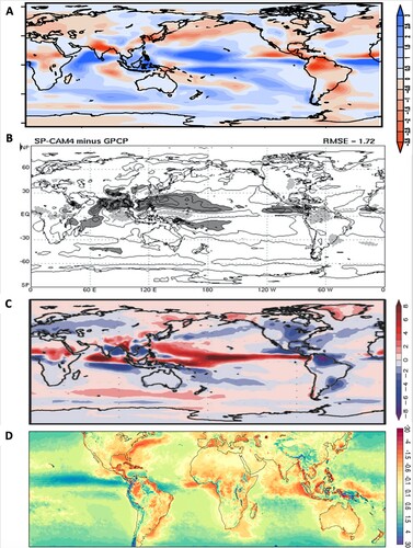
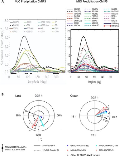
Fig. 3 (A) MJO precipitation variance in CMIP3 models (left, from Lin et al., 2006) and CMIP5 models (right, from Hung et al., 2013). (B) Phase and amplitude of diurnal cycle of precipitation over land (left) and ocean (right) for CMIP5 AMIP models and TRMM observations (adapted from Covey et al., 2016).

Table 1 summarizes the convection schemes used in global and regional climate models grouped by the types of closure assumptions. The biases in global cloud-resolving models and models with super-parameterization suggest that atmospheric convection is not only a resolution problem. In the foreseeable future, supercomputers will not be able to conduct long-term (e.g. 100 years and longer) ensemble global cloud-resolving model runs, although such runs are basic requirements for understanding global climate and climate change. Therefore, improving convective parameterization is very important at the current stage and in the foreseeable future.

Table 1 Convection schemes used in global and regional models grouped by closure assumptions.

Closure	First-Generation Scheme	Later Schemes	Models	Other Models
Moisture Convergence	Kuo (1965, 1974)	Bougeault (1985) Frank and Cohen (1987) Tiedtke (1989) Grell (1993), Grell and Devenyi (2002) Freitas et al. (2021)	Centre National de Recherches Météorologiques, France PSU/NCAR Mesoscale Model European Centre for Medium-Range Weather Forecasts Max Planck Institute for Meteorology, Germany NCAR Weather Research and Forecasting Model NOAA National Center for Environmental Prediction NASA Global Modeling and Assimilation Office NOAA Global Systems Laboratory NCAR Weather Research and Forecasting Model NCAR Regional Climate Model	Irish Centre for High-End Computing
Flux-type CQE	Arakawa and Schubert (1974)	Moorthi and Suarez (1992) Donner (1993) Randall and Pan (1993) Grell (1993), Grell and Devenyi (2002) Freitas et al. (2021) Zhang and McFarlane (1995) Chikira and Sugiyama (2010) Wu (2012) Zhao et al. (2018)	Geophysical Fluid Dynamics Laboratory Geophysical Fluid Dynamics Laboratory Model for Interdisciplinary Research on Climate, Japan Meteorological Research Institute, Japan Same as above National Center for Atmospheric Research Canadian Centre for Climate Modelling and Analysis, Canada Model for Interdisciplinary Research on Climate, Japan Beijing Climate Center, China Geophysical Fluid Dynamics Laboratory	Bjerknes Centre for Climate Research, Norway Institute of Atmospheric Physics, China Academia Sinica, Taiwan
State-type CQE	Manabe et al. (1965)	Fritsch and Chappell (1980) Betts (1986) Kain and Fritsch (1990) Gregory and Rowntree (1990) Emanuel (1991) Del Genio and Yao (1993) Grell (1993), Grell and Devenyi (2002) Freitas et al. (2021) Yoshimura (2015)	PSU/NCAR Mesoscale Model Institute of Numerical Mathematics, Russia NCAR Weather Research and Forecasting Model Met Office Hadley Center, United Kingdom Institute Pierre-Simon Laplace, France NASA Goddard Institute for Space Studies Same as above Meteorological Research Institute, Japan	Commonwealth Scientific and Industrial Research Organization, Australia

The purpose of this paper is to review the observational constraints for convective parameterization and the most widely used convection schemes. Section 2 will review the observational studies of atmospheric convection. Section 3 will review the ECMWF convection scheme, which evolved from the Tiedtke scheme with moisture convergence closure. Section 4 reviews the Grell scheme with flux-type quasi-equilibrium closure, which is used in the National Center for Environmental Prediction (NCEP) GFS model, the NOAA GSL model, and the regional Weather Research and Forecast (WRF) model. Section 5 reviews the Zhang-McFarlane scheme with flux-type quasi-equilibrium closure, which is used in the National Center for Atmospheric Research (NCAR) and the US Department of Energy climate models. Section 6 reviews the parametrization of shallow moist convection. A summary of current challenges and suggested future directions is given in Section 7.

2 Observations of atmospheric convection

a Cloud Structure

Atmospheric convection can be divided into deep convection and shallow convection. Deep convective systems are thunderstorms, which include ordinary thunderstorms, multi-cell thunderstorms and supercell thunderstorms, and mesoscale convective systems (MCSs), which include squall lines and mesoscale convective complexes (MCCs). Shallow convection refers to cumulus clouds, which are also called fair weather cumulus or trade wind cumulus, and stratocumulus clouds.

Soon after the invention of basic modern meteorological instruments, such as rain gauge, anemometer, thermometer and barometer, scientists started to observe the surface structure of thunderstorms, especially sudden increase of wind speed and sudden drop of air temperature, which are likely downdrafts and cold pools (e.g. Planer, 1782; Rosenthal, 1786; Strehlke, 1830; Symons, 1890; Toaldo, 1794). Cold pool is a cold pocket of dense air that forms when rain evaporates during intense precipitation inside downdrafts underneath a thunderstorm cloud. Cold pools propagate away from the rain event along the surface as a moving gust front. When the gust front passes, cold pools cause a sudden increase in wind speed and a sudden drop in specific humidity and in air temperature. In 1857, G. J. Symons established an organization to study the English thunderstorms (Symons, 1889). In 1887, the Royal Meteorological Society set up a committee to study thunderstorms, and published two summary reports (Abercromby, 1888; Mareiott, 1890). Using 10 years (1925-1934) of data from surface station network, Ward (1936) constructed composite surface conditions for different types of thunderstorms. Four distinct types of pressure distribution were identified as giving rise to thunderstorms on the national forests of the Pacific Northwest. Listed according to their frequency and forecasting importance, they are: Type I. Trough; Type II. Cyclonic; Type III. Transition; Type IV. Border. With data from the earliest upper air sounding network, Neiburger (1941) analyzed the potential vorticity field of a thunderstorm.

MCSs, such as squall lines, were also discovered from surface measurements in the nineteenth century (e.g. Hinrichs, 1883, 1888a, 1888b; Ley, 1878, 1883; Stewart, 1863). Stewart (1863) noted that a sudden squall occurred almost simultaneously at Oxford and Kew, UK, which are 53 miles away from each other. He documented “a very sudden increase of pressure accompanied with a violent gust of wind”, which was a cold pool associated with convective downdrafts. Hinrichs (1883) presented nice charts of the propagation of squall lines, which he later named derechos (Hinrichs, 1888a, 1888b). Ley (1883) linked these continental squall lines to their oceanic counterparts known to English seaman, who bestowed the name “arched squalls” to all squalls which are seen in perspective to rise as arches of cloud above the horizon. The upper air structure of squall lines was examined using sounding data (Giblett, 1923; Hamilton & Archbold, 1945; Newton, 1950). Observational studies also began on stratocumulus clouds (Sverdrup, 1917; Wyatt, 1923) and trade wind cumulus clouds (Ficker, 1936; Riehl et al., 1951).

World War II led to the birth of radar meteorology (Bent, 1946; Maynard, 1945; Ryde, 1946; Wexler, 1947; Wexler & Swingle, 1947), which, together with the use of aircraft reconnaissance, made it possible to study the three-dimensional dynamical structure of convective systems. Surface precipitation was estimated using Z-R relationships (Laws & Parsons, 1943; Wexler, 1948). Maynard (1945) presented radar echoes for various types of convective systems obtained during World War II. The 1946–1947 Thunderstorm Project, which was one of the largest field experiments in the history of atmospheric sciences, integrated surface stations, upper air soundings, radar, and aircraft reconnaissance to study the dynamical structures of ordinary and multi-cell thunderstorms (Byers et al., 1946; Byers & Battan, 1949; Byers & Braham, 1948; Byers & Hull, 1949; Byers & Rodebush, 1948). Soon after, radars were used to study severe supercell thunderstorms (Stout & Huff, 1953) and MCSs (Ligda, 1956).

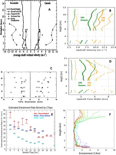
Since then, numerous field projects have been conducted, which have significantly advanced our knowledge and understanding of atmospheric convection. The whole atmospheric convection process is initiated by convective updrafts, which are driven by positive buoyancy force, but suppressed by entrainment of dry environmental air. The basic parameters for convective updrafts are size, vertical velocity, and entrainment rate. The size and vertical velocity of convective updrafts have been measured using aircraft flight level data and vertically pointing radars (Black et al., 1996; Giangrande et al., 2013, 2016; Jorgensen et al., 1985; Jorgensen & LeMone, 1989; LeMone & Zipser, 1980; Lucas et al., 1994; May & Rajopadhyaya, 1999; Wang et al., 2020a; Zipser & LeMone, 1980). Convective updrafts over land have a larger size and stronger vertical velocity than those over ocean. The strongest 10% updrafts have an average vertical velocity of ∼4 m/s over ocean, but >8 m/s over land (Fig. 4a,b). The width is ∼2 km over ocean and 3–4 km over land (Fig. 4c,d). Entrainment of lower/middle troposphere air is the leading factor controlling cloud-top height (Brown & Zhang, 1997; Jensen & Del Genio, 2006; Stanfield et al., 2019; Wang et al., 2020b). There are few undiluted updrafts in nature. Brown and Zhang (1997) found that the cloud-top heights of deep convection in TOGA COARE are much lower than those predicted using simple undiluted updrafts, but better explained by an entraining updraft model. Wang et al. (2020) found that the cloud-top heights observed by cloud radar in six ARM tropical sites are 2–8 km lower than those predicted using undiluted updrafts. Using global cloud-top heights observed by CloudSat/CALIPSO and associated carbon monoxide measurements, Stanfield et al. (2019) estimated that the entrainment rate is between 15%/km and 50%/km for deep convection around the world (Fig. 4e). The vertical profiles of entrainment rate have been estimated from cloud-resolving model simulations (Becker et al., 2018; Becker & Hohenegger, 2021; de Rooy et al., 2013; Del Genio & Wu, 2010; Gu et al., 2020; Hannah, 2017; Lu et al., 2018; Romps, 2010; Zhang et al., 2016). Zhang et al. (2016) found that for each cloud category, the entrainment rate is high near cloud base and top, but low in the middle of clouds (Fig. 4f). Becker et al. (2018) found that in the lower free troposphere the bulk entrainment rate increases when convection aggregates, which is against the hypothesis that convective updrafts surrounded by pre-existing convection are undiluted.

Fig. 4 (A) Average vertical velocity in the strongest 10% convective updrafts and downdrafts in oceanic convection comparing with Florida Thunderstorm Project data (from Black et al., 1996). (B) Average vertical velocity in the strongest 10% convective updrafts in Amazon and Southern Great Plain (SGP) (from Wang et al. 2020). (C) Same as A but for convective core width (from Lucas et al., 1994). (D) Same as B but for convective core width. (E) Global estimated entrainment rate binned by cloud top heights (from Stanfield et al., 2019). (F) Vertical profile of entrainment rate for TWP-Ice in Australia (from Zhang et al., 2016).

Many studies have added stochastic processes to convective updrafts using Monte Carlo buoyancy sorting parcels (Emanuel, 1991; Grandpeix et al., 2004; Raymond & Blyth, 1986), stochastically perturbed parameters (Grell & Devenyi, 2002; Grell & Freitas, 2014; Leutbecher et al., 2017), stochastic mass flux distribution (Keane et al., 2014, 2016; Keane & Plant, 2012; Plant & Craig, 2008; Wang & Zhang, 2016), stochastic entrainment (Romps, 2016; Romps & Kuang, 2010; Suselj et al., 2013), stochastic size distribution (Hagos et al., 2018), stochastic cloud types (Goswami et al., 2017; Khouider et al., 2010; Peters et al., 2017), and stochastic triggers (D’Andrea et al., 2014; Rio et al., 2009, 2013; Rochetin et al., 2014a, 2014b). In general, stochastic processes enhance the sway of the convection scheme. Due to the nonlinear nature of convection, expansion of the distribution may make convection more difficult to occur (Wang et al., 2016), enhance the variability of precipitation (Goswami et al., 2017; Peters et al., 2017), and postpone the precipitation maximum in the diurnal cycle (Rio et al., 2009, 2013). There are other modifications related to convective updrafts such as explicit calculation of updraft velocity and chemical transport (Donner, 1993; Donner et al., 2001, 2016; Jeevanjee & Romps, 2015; Lee et al., 2009; Morrison, 2016a, 2016b; Peters, 2016; Simpson & Wiggert, 1969), scale-aware parameters (Freitas et al., 2020; Grell & Freitas, 2014; Han et al., 2017b), machine learning (Gentine et al., 2018; O'Gorman & Dwyer, 2018; Schneider et al., 2017), and unified treatment of boundary layer, shallow convection and deep convection (D’Andrea et al., 2014; Park, 2014a, 2014b). See Rio et al. (2019) for a review of recent studies.

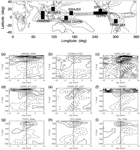
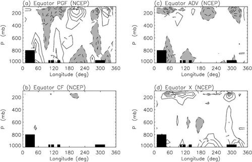
Triggering is generally needed for convective updrafts to happen, since the environment for atmospheric convection is usually conditionally unstable with convective inhibition. When entrainment effect is considered, free convection is further suppressed and initial trigger is even more important. Mapes and Lin (2005) analyzed the life cycle of deep convective systems in seven tropical field experiments and found that boundary layer convergence always leads deep convection by a few hours (Fig. 5). Vertical motion associated with boundary layer convergence can push the air parcel passing the lifting condensation level and achieving positive buoyancy. Coincidently, the two IPCC AR4 models that produced the best MJO simulations were the only ones having moisture convergence closure/trigger (Lin et al., 2006). There are also subgrid-scale triggers such as the density currents from convective downdrafts and low-level gravity waves.

Fig. 5 Lag-regression of divergence profile with respect to surface precipitation for seven field experiments. Lag 0 is the time of maximum precipitation, and lag −10 (+10) hours means 10 h before (after) maximum precipitation. The locations of the field experiments are shown in the top map (from Mapes & Lin, 2005).

The convective downdrafts include negatively buoyant downdrafts and positively buoyant downdrafts. Low-level downdrafts are often unsaturated and have negative buoyancy caused by precipitation loading, evaporation and melting (Knupp & Cotton, 1985). When touching down at the ground, the convective downdrafts in deep convection significantly decrease the boundary layer entropy, and thus suppress the local development of new convection (Barnes & Garstang, 1982; Das & Subba Rao, 1972; de Szoeke et al., 2017; Engerer et al., 2008; Jabouille et al., 1996; Johnson & Nicholls, 1983; Kamburova & Ludlam, 1966; Saxen & Rutledge, 1998; Schiro & Neelin, 2018; Young et al., 1995; Zipser, 1977). It is important to note that although Zipser (1977) suggested that the convective downdrafts are saturated, most of the other studies showed that the convective downdrafts are unsaturated, which is likely because the precipitation particles do not have enough time to evaporate. LES simulations also supported that the convective downdrafts are unsaturated (Hohenegger & Bretherton, 2011; Torri & Kuang, 2016). Convective downdrafts also enhance surface fluxes in convective wakes, which contribute to boundary layer recovery and accumulation of convective instability. The cold pools may also affect future convective organization and vertical structure (Holloway et al., 2017; Tobin et al., 2012). Upper-level warm downdrafts not driven by precipitation or evaporation have been observed in both thunderstorms (Kingsmill & Wakimoto, 1991; Knupp, 1987, 1988; Raymond et al., 1991; Yuter & Houze, 1995a, 1995b, 1995c) and MCSs (Heymsfield & Schotz, 1985; Smull & Houze, 1987; Sun et al., 1993). Sun et al. (1993) conducted thermodynamic retrievals using Doppler radar data and found that the upper-level downdrafts next to convective updrafts are generally positively buoyant. Warm low-level downdrafts with positive buoyancy have also been observed by aircraft flight-level measurements (Igau et al., 1999; Jorgensen & LeMone, 1989; Lucas et al., 1994). The positively buoyant warm downdrafts likely result from the pressure gradient forces required to maintain mass continuity in the presence of adjacent buoyant updrafts (Feynman et al., 1965; Yuter & Houze, 1995b).

Atmospheric convection often occurs in the form of well-organized convective systems. The detailed structures of deep convective systems are shown in Fig. 6. The ordinary thunderstorms generally go through three stages in their lifecycle: the developing stage, mature stage, and dissipating stage (Fig. 6a; Byers & Braham, 1948). In the developing stage the storm is formed from an updraft of air which, as in the other stages, entrains air from the environment. In this stage no rain has yet reached the ground. In the mature stage, rain is occurring, and a large part of the storm consists of a downdraft which characterizes the rain area. The updraft continues in a portion of the storm in the low and intermediate levels and in all parts of the top levels. In the dissipating stage, downdrafts are present throughout, although weak upward motion still exists in the upper levels. Fig. 6a can also be viewed as a schematic of the multi-cell thunderstorm, which shows three cells lining up side by side, and downdrafts from the old mature or dissipating cells triggering new developing cells in the nearby region.

Fig. 6 (A) Circulation within an ordinary thunderstorm in (left) developing, (middle) mature, and (right) dissipating stages (adapted from Byers & Braham, 1948). (B) Visual model of the mature phase of a classic supercell thunderstorm (adapted from Bluestein & Parks, 1983). (C) Vertical cross-section of an MCC (adapted from Fortune et al., 1992). (D) Schematic cross-section of a squall line moving from right to left, and the post-convection sounding. Circled numbers are typical values of θw in °C (adapted from Zipser, 1977).

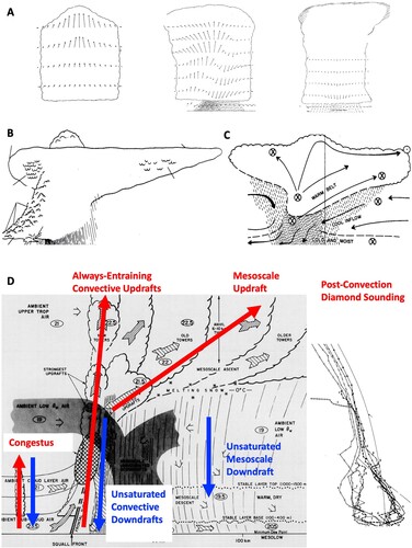
The supercell thunderstorm is characterized by a persistent, deep, 2–10 km wide, rotating updraft in strong vertical wind shear, which is associated with forward-flank and rear-flank downdrafts (Bluestein & Parks, 1983; Browning, 1964; Fujita, 1958; Lemon & Doswell, 1979; Markowski, 2002; Markowski et al., 2018; Markowski & Richardson, 2009; Markowski & Straka, 2002; Marquis et al., 2008; Wakimoto & Liu, 1998). Fujita (1958) suggested that the tornadic supercell thunderstorms resemble a miniature hurricane with a central eye and spiral echo bands. Lemon and Doswell (1979) found that the structure of supercell storms is similar to a miniature occluded extratropical cyclone. Bluestein and Parks (1983) showed the vertical structure of classic supercell thunderstorms (Fig. 6b). The storm has a penetrating convective cloud top and wide anvil clouds, all tilting downshear and generating precipitation underneath. Wall clouds and tornado generally form upshear, close to the rear-flank downdrafts.

The MCCs show a wide spectrum of structures from chaotic systems to well-organized systems (Augustine & Howard, 1988; Blanchard, 1990; Cotton et al., 1989; Fortune et al., 1992; Kane et al., 1987; Leary & Rappaport, 1987; Maddox, 1980, 1983; McAnelly & Cotton, 1989; Smull & Augustine, 1993; Wetzel et al., 1983). The structure of well-organized MCCs is similar to a small occluded extratropical cyclone with a warm conveyer belt and a cold conveyer belt (Fortune et al., 1992). An MCC is composed of the same four components as a squall line, although the stratiform precipitation exists in a broad region surrounding the convective cores rather than trailing the convective line (Fig. 6c). In the early stage, thunderstorm-scale motions and strong convective precipitation prevail, while in the mature stage, light stratiform precipitation reaches maximum horizontal extent leading to maximum precipitation amount. Then the system slowly decays, producing lighter and lighter rainfall.

The squall lines have been examined extensively by many field experiments (e.g. Bluestein & Jain, 1985; Bryan & Parker, 2010; Gallus & Johnson, 1991, 1992; Grim et al., 2009; Houze, 1977; Houze et al., 1989; Johnson & Hamilton, 1988; Roux et al., 1984; Scott & Rutledge, 1995; Weisman, 2001; Zipser, 1977). As shown by Zipser (1977; Fig. 6d), a squall line has four components: the convective updraft, convective downdraft, mesoscale updraft, and mesoscale downdraft. In general, these four components are also the building blocks of all convective systems. The convective downdraft brings low entropy air into the boundary-layer and suppresses the convective instability, while the mesoscale downdraft warms up and dries up the lower troposphere above the boundary-layer, both of which lead to a “diamond sounding” and suppress the development of future deep convection. Gamache and Houze (1983) calculated the water budget of a tropical squall line and found that the mesoscale updraft accounts for 25–40% of the stratiform precipitation, while the remaining 60–75% is supplied by horizontal transport of condensate generated in the convective updrafts. During their lifetime, squall lines tend to evolve from a symmetric configuration to an asymmetric configuration with bow echo or comma echo (Scott & Rutledge, 1995; Weisman, 2001).

Self-aggregation of convection, the spontaneous organization of initially scattered convection into isolated convective clusters under homogeneous boundary conditions and forcing, has been found in numerous modelling studies (e.g. Bretherton et al., 2005; Held et al., 1993; Muller & Held, 2012; Wing et al., 2017). The formation mechanisms in the models include longwave radiation, shortwave radiation, surface fluxes, moisture feedbacks and advective processes (Wing et al., 2017). However, there is limited observational evidence of convective self-aggregation (Holloway et al., 2017; Tobin et al., 2012; Zuidema et al., 2017), and whether it needs to be specially parameterized needs further studies (Tobin et al., 2013).

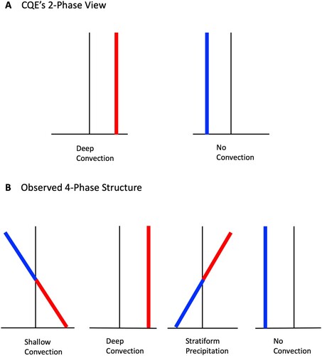
Overall, the convective systems have four components: the always-entraining convective updrafts, unsaturated convective downdrafts, mesoscale updrafts and mesoscale downdrafts (Fig. 6d). The observed convection has self-suppression mechanisms caused by entrainment in convective updrafts, surface cold pool generated by convective downdrafts, and warm and dry lower troposphere created by mesoscale downdrafts. The post-convection environment is often characterized by “diamond sounding”, which suggests an over-stabilization of the atmosphere rather than barely returning to the neutral state. Then the pre-convection environment for the future events is characterized by slow moistening of the lower troposphere forced by moisture convergence and surface fluxes. The over-stabilization and slow moistening make the convection events episodic.

As summarized by Lin et al. (2006, 2015) and Lin (2007), there are some parametrization schemes still using undiluted convective updrafts either in the cloud ensemble or in the convective trigger. The undiluted convective updrafts will ignore the suppression effect of a dry lower troposphere, skip the slow pre-conditioning process associated with the development of shallow convection, and lead to an unrealistic quasi-equilibrium state. Possible modifications include setting up a minimum entrainment rate for the cloud ensemble (Tokioka et al., 1988) and using a strong, possibly relative humidity or buoyancy dependent, entrainment (Bechtold et al., 2014; Derbyshire et al., 2004). Such modifications will suppress deep convection and may cause cold temperature biases in the upper troposphere (Gates et al., 1999; John & Soden, 2007; Tian et al., 2013). Adding mesoscale updrafts will warm up the upper troposphere as in nature.

In most convection schemes, the convective downdrafts are saturated, and need to be modified to unsaturated downdrafts. Betts and Silva Dias (1979) and Emanuel (1981) developed models for unsaturated downdrafts, while Emanuel (1991) is the only scheme using unsaturated convective downdrafts. Parameterizations of mesoscale enhancement of surface fluxes have been developed by Qian et al. (1998) and Redelsperger et al. (2000). Parameterizations have also been developed on how convective downdrafts trigger new convection and affect convective organization (Grandpeix et al., 2010; Grandpeix & Lafore, 2010; Mapes & Neale, 2011).

Only one convection scheme has explicitly considered the mesoscale updrafts and downdrafts (Donner, 1993; Donner et al., 2001, 2011; Wilcox & Donner, 2007), although various ideas have been proposed on how to parameterize the mesoscale effects (Alexander & Cotton, 1998; Khouider & Moncrieff, 2015; Mapes & Neale, 2011; Moncrieff et al., 2017; Yano & Moncrieff, 2016, 2018). There are indications that incorporating mesoscale heating structure can drastically improve the simulation of intraseasonal variability such as MJOs in climate models (Cao & Zhang, 2017). The mesoscale heating/moistening structures are quite simple and consistent around the world (Fig. 8a,b). The key unanswered question is what controls the fraction of stratiform precipitation. Observational studies suggested that wind shear and upper-troposphere moisture enhance the formation of anvil clouds and stratiform precipitation (Hogan & Illingworth, 2003; Lin & Mapes, 2004; Saxen & Rutledge, 2000). Cloud-resolving models have a long-lasting bias of underestimating stratiform precipitation and anvil cloud area (Fovell & Ogura, 1988; Franklin et al., 2016; Fridlind et al., 2017; Han et al., 2019; Lang et al., 2003; Luo et al., 2010; McCumber et al., 1991; Morrison et al., 2015; Varble et al., 2011, 2014; Wu et al., 2013).

b Bulk Effects

The amount of surface precipitation represents column-integrated latent heating. Figure 7a shows the GPCP climatological annual mean precipitation for 1981–2010. The largest precipitation is over the tropical continents, Indo-Pacific warm pool, and the tropical/subtropical convergence zones, such as the ITCZ, Mei-Yu, and SPCZ. Satellites provide excellent data for studying climatology of tropical deep convection (Houze et al., 2015; Liu et al., 2007; Liu & Zipser, 2005, 2015; Yuan & Houze, 2010; Zipser et al., 2006). Extremely deep and intense convective elements occur almost exclusively over land, while shallow isolated raining clouds are overwhelmingly an oceanic phenomenon. Continental MCSs tend to have stronger convective regions, with some of the strongest convective regions occurring near the tropical great mountains. Oceanic systems mesoscale convective systems tend to have weaker convective regions but wider stratiform regions. Yuan and Houze (2010) found that the distribution of MCSs is similar to the distribution of total rainfall. MCSs contribute 56% of tropical rainfall, which implies that isolated thunderstorms contribute less than 44% of tropical rainfall. Partitioning between the two types of MCSs have been conducted for the United States (Anderson & Arritt, 1998; Jirak et al., 2003). Using 3 years of data, Jirak et al. (2003) found that 61% of MCSs in the United States were squall lines, and 39% were MCCs. Their data showed that the total amount of rainfall produced by the squall lines double that of MCCs. Over the globe, MCCs mainly occur over land (Laing & Fritsch, 1997). During warm seasons, MCCs contribute 21–26% of total rainfall in western Africa (Laing et al., 1999), 8–18% of total rainfall in central United States (Ashley et al., 2003), 15–21% in central South America (Durkee et al., 2009) and 10–20% in eastern South Africa (Blamey & Reason, 2013). Future studies are needed to partition rainfall of isolated thunderstorms into contribution from different types of thunderstorms (ordinary, multi-cell and supercell).

Fig. 7 (A) The GPCP climatological mean precipitation (contour interval 1.5 mm/day). The coloured boxes are regions used in b and c. (B) Normalized vertical distribution of TRMM precipitation radar 20 dBZ echo top for convective precipitation from 16 years of data (1998–2013). (C) Normalized Q₁ profiles for NAME, TOGA COARE, DYNAMO and GATE.

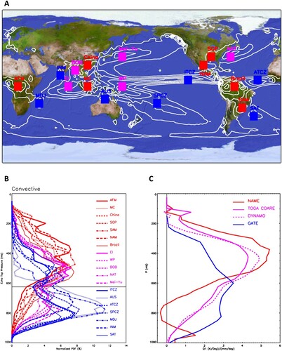
The distribution of deep convective cloud tops exhibits three regimes (Fig. 7b): the continental deep convection, oceanic deep convection, and oceanic congestus convection. The oceanic congestus convection was first discovered by Johnson et al. (1999) over western Pacific warm pool during the pre-conditioning stage of deep convection. Here we found that congestus convection occurs throughout the tropical and subtropical convergence zones over medium sea surface temperature. For example, the tropical eastern Pacific ITCZ has the strongest climatological mean surface precipitation, but the cloud top of deep convection is much lower than over the western Pacific warm pool. The same feature occurs over the eastern Atlantic ITCZ where the GATE experiment was conducted.

The TRMM radar echo top distributions are confirmed by the vertical heating profiles observed during field experiments. The vertical heating profile of atmospheric convection can be derived from heat budgets using sounding array or reanalysis datasets (e.g. Frank et al., 1996; Frank & McBride, 1989; Johnson et al., 2007, 2015; Lin et al., 2004; Lin & Johnson, 1996; Thompson et al., 1979; Yanai et al., 2000). The methods for deriving apparent heat source Q₁ and moisture sink Q₂ were summarized by Yanai and Johnson (1993). Zhang and Lin (1997) later developed a constrained variational analysis method to make the mass, heat, moisture and momentum budgets self-consistent. Figure 7c shows the Q₁ profiles from NAME, TOGA COARE, DYNAMO and GATE, which clearly demonstrate the three regimes of tropical deep convection. It is important to note that deep convection observed during GATE represents the congestus regime, which is different from the deep convection in TOGA COARE/DYNAMO.

The stratiform precipitation is associated with a universally consistent cloud top distribution (Fig. 8a). Q₁ profile in stratiform region is characterized by heating in the upper troposphere, but cooling in the lower troposphere (Houze, 1982, 1997; Johnson & Young, 1983). Given the standard Q₁, Q₂ profiles associated with stratiform precipitation, any Q₁, Q₂ profile could be partitioned into a convective component and a stratiform component provided that the stratiform rainfall fraction and radiative heating profile are known (Fig. 8b; Johnson, 1984; Lin et al., 2004).

Fig. 8 (A) Normalized vertical distribution of TRMM precipitation radar 20 dBZ echo top for stratiform precipitation for regions shown in Fig. 7A. (B) Partitioning of GATE Q₁ profile into convective, stratiform and radiative components (from Johnson, 1984). (C) TRMM PR convective and stratiform precipitation fractions for NH summer (from Yang & Smith, 2008). (D) CMIP5 model convective precipitation fraction for high-resolution and low-resolution ensemble means for NH summer (from Huang et al., 2018).

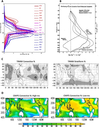
The stratiform precipitation contributes significantly to the tropical precipitation and thus the total latent heating (Schumacher & Houze, 2003; Yang & Smith, 2008; Fig. 8c). Over the tropical oceanic convection centres such as the Indo-Pacific warm pool, ITCZ and SPCZ, the stratiform precipitation fraction is about 40–50%, and the convective precipitation fraction is also 40–50%. Over tropical continents, the stratiform precipitation fraction is about 30–40%, while the convective precipitation fraction is about 60–70%. The global climate models significantly underestimate the stratiform precipitation fraction with most precipitation being convective (Dai, 2006; Huang et al., 2018; Fig. 8d). The CMIP5 low-resolution models produce ∼90% convective precipitation fraction over tropical oceans and continents. The high-resolution models have improved simulations, but still produce >70% convective precipitation fraction over tropical oceans (Huang et al., 2018). The stratiform precipitation in climate models is produced by the large-scale condensation schemes or partly from detrained convective condensate. However, the stratiform heating profile might be different from the observed stratiform heating profile with upper-troposphere heating and lower-troposphere cooling, which is important for generating the “diamond sounding” and suppressing future convection.

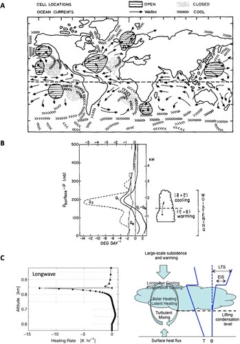
The regions free of deep convection in Fig. 7a (with <1.5 mm/day climatological mean precipitation) are generally covered by shallow cumulus and stratocumulus clouds (Agee et al., 1973; Agee, 1987; Fig. 9a). In cold seasons, the Mei-Yu front region and Gulf Stream front region are also covered by shallow cumulus clouds. There is a transition from deep convection to cumulus, then to stratocumulus when we move from the ascending branch to the descending branch of Hadley circulation and/or Walker circulation. The mesoscale organization tends to be open cells in cumulus clouds, closed cells in stratocumulus clouds, and no cellularity in the polar/subpolar stratus clouds. The heat and moisture budgets of trade wind cumulus have been calculated using sounding array data from several field experiments (Augstein et al., 1973; Betts, 1975; Brummer, 1978; Esbensen, 1975; Johnson & Lin, 1997; Nitta & Esbensen, 1974; Fig. 9b). The Q₁ profile is characterized by warming in the subcloud layer where vertical eddy heat flux convergence exceeds radiative cooling, and cooling in the upper cloud layer caused by radiative cooling and evaporation of condensate. The Q₂ profile shows moistening in the subcloud layer caused by surface evaporation, and strong moistening in the upper cloud layer caused by the evaporation of cloud water. The longwave heating profile is characterized by a strong cooling at cloud top (Larson et al., 2007; Slingo et al., 1982; Fig. 9c). Vertical velocity in trade wind cumulus has been studied using aircraft data, which increases with height in both updrafts and downdrafts and has a magnitude of ∼0.5–2 m/s (Ghate et al., 2010, 2011; Kollias & Albrecht, 2010; Lamer et al., 2015).

Fig. 9 (A) Global climatology of mesoscale cellular convection depicting the most favoured regions of open and closed mesoscale cellular convection over the oceans (from Agee, 1987). (B) Left: The observed Q₁, Q₂, Q_R, and Q₁ − Q_R for the undisturbed BOMEX period 22–26 June 1969 (from Nitta & Esbensen, 1974). Right: Schematic of trade wind cumulus layer showing effects of condensation c and evaporation e on the heat and moisture budgets (from Johnson & Lin, 1997). (C) Left: Longwave heating rate of a stratocumulus-topped boundary layer (from Larson et al., 2007). Right: Schematic depiction of the large-scale forcing and physical processes for a stratocumulus-topped boundary layer. LTS is lower troposphere stability and EIS is estimated inversion strength (adapted from Lin et al., 2014).

Numerous field experiments have been conducted to study shallow cumulus clouds and stratocumulus clouds (Albrecht et al., 1985, 1988, 1995, 2019; Austin et al., 1996; Bretherton et al., 2004b; Brocks, 1972; Curry et al., 2000; Keuttner & Holland, 1969; Lenschow et al., 1988; Lu et al., 2007; Paluch, 1979; Stevens et al., 2003; Verlinde et al., 2007; Wood et al., 2011; Zuidema, 2018; Zuidema et al., 2016). For the stratocumulus-topped boundary layer (STBL, Fig. 9b), convective instability and turbulence are driven mainly by the cloud-top longwave cooling and evaporative cooling, which are partially reduced by shortwave warming and latent heating inside the cloud layer, and the resulting STBL turbulence is enhanced by latent heating in updrafts and cooling in downdrafts. Turbulent eddies and evaporative cooling drives entrainment at the top of the STBL, which tends to deepen the STBL, maintaining it against large-scale subsidence. Drizzle reduces the liquid water path and albedo and can lead to increased mesoscale variability, stratification of the STBL, and in some cases cloud breakup. For a given cloud thickness, polluted clouds tend to produce more and smaller cloud droplets, greater cloud albedo, and drizzle suppression. Feedbacks between radiative cooling, precipitation formation, turbulence, and entrainment help regulate stratocumulus. The stratocumulus cloud cover is well correlated with the lower troposphere stability (LTS) and estimated inversion strength (EIS), both of which are measures of the temperature inversion strength (Klein & Hartmann, 1993; Norris, 1998; Slingo, 1987; Wood & Bretherton, 2006). The liquid water path of the SEP stratocumulus clouds is often close to the adiabatic value, and thus determined by cloud thickness (Zuidema et al. 2005, 2012; Bretherton et al. 2004, 2010). The cloud thickness is primarily maintained by a strongly negative cloud-radiation-turbulent-entrainment feedback (Zhu et al., 2005), and the thickness could vary due to changes in turbulent driving, vertical gradient of moisture and moist static energy, large-scale subsidence, and inversion strength (Brient & Bony, 2013; Bretherton et al., 2013; Caldwell & Bretherton, 2009; Zhang & Bretherton 2008; Zhu et al., 2007).

In global climate models, shallow cumulus clouds are treated either together with deep convection by a single convection scheme, or by a separate shallow convection scheme. Stratocumulus clouds, on the other hand, are treated by the PBL scheme coupled with microphysics and radiation schemes. PBL schemes have evolved through three stages: (1) local schemes (e.g. Louis, 1979) relating the diffusivity to the local stability, which work well for stable conditions but not for unstable conditions; (2) nonlocal schemes (e.g. Holtslag & Boville, 1993) with nonlocal diffusivity whose magnitude is determined by surface forcing, which works well for unstable conditions driven by surface forcing but not for unstable conditions driven by forcing from boundary layer top, such as the stratocumulus-topped boundary layer; and (3) nonlocal schemes with consideration of cloud-top forcing (e.g. Bretherton & Park, 2009; Grenier & Bretherton, 2001; Lock et al., 2000; van Meijgaard & van Ulden, 1998). Lin et al. (2014) examined the stratocumulus clouds and associated cloud feedback in the southeast Pacific simulated by eight CMIP5/CFMIP global climate models and found that two models could capture the observed stratocumulus clouds and associated cloud feedback, which are the only ones using cloud-top radiative cooling to drive boundary layer turbulence.

Convective momentum transport has been diagnosed for various convective systems using sounding array or reanalysis datasets (Gallus & Johnson, 1992; Hsu & Li, 2011; LeMone et al., 1984; LeMone & Moncrieff, 1994; Lin et al., 2005, 2008; Stevens, 1979; Sui & Yanai, 1986; Tung & Yanai, 2002a, 2002b; Wu & Yanai, 1994; Zhang & Lin, 1997). Wu and Yanai (1994) analyzed the momentum budget of MCSs during SEASAME and PRE-STORM experiments and found that convective momentum transport is downgradient in MCCs, but upgradient in the upper level of squall lines for momentum normal to the squall line. Stevens (1979) analyzed the momentum budget of easterly waves during GATE and found that convective momentum transport is an important term in the meridional momentum budget. Lin et al. (2005) calculated the zonal momentum budget for the MJO, but found that convective momentum transport is not a leading term in MJO’s momentum budget. However, Lin et al. (2008) examined the zonal momentum budget of the Walker Circulation (Fig. 10), and discovered that convective momentum transport, together with pressure gradient force, are the two leading forces driving the Walker Circulation. Convective momentum transport has not been included in many convection schemes. The inclusion of convective momentum transport (Zhang & Cho, 1991) in a GCM showed that it had significant effects on the Hadley circulation (Zhang & McFarlane, 1995b). Therefore, including convective momentum transport in convection schemes is very important for simulating a realistic tropical mean climate.

Fig. 10 Zonal momentum budget of the Walker Circulation, as shown by climatological annual mean (a) pressure gradient force, (b) Coriolis force, (c) advective tendency, and (d) convective eddy momentum flux convergence along the equator (5N-5S) derived from 15 years (1979–1993) of NCEP reanalysis data. Unit is m/s/day (from Lin et al., 2008).

c Closure Assumption

A convection scheme generally has two aspects: the cloud model and the closure assumption. Because the closure assumption determines when the convection will happen and how strong the convective fluxes will be, it is generally considered as a more fundamental characteristic of a convection scheme. The closure assumptions of existing convection schemes can be categorized into three groups (Table 1): (1) moisture convergence (Anthes, 1977; Bougeault, 1985; Frank & Cohen, 1987; Krishnamurti et al., 1976; Kuo, 1965, 1974; Molinari, 1985; Tiedtke, 1989); (2) flux-type convective quasi-equilibrium (CQE) (Arakawa & Schubert, 1974; Bechtold et al., 2014; Chikira & Sugiyama, 2010; Donner, 1993; Emanuel, 1995; Grell, 1993; Grell & Devenyi, 2002; Moorthi & Suarez, 1992; Randall & Pan, 1993; Raymond, 1995; Wu, 2012; Zhang, 2002; Zhang & McFarlane, 1995; Zhang & Wang, 2006; Zhao et al., 2018). (3) state-type CQE (Betts, 1986; Emanuel, 1991; Emanuel et al., 1994; Fritsch & Chappell, 1980; Gregory & Rowntree, 1990; Kain, 2004; Kain & Fritsch, 1990, 1992; Khouider & Majda, 2006; Kuang, 2008; Majda & Shefter, 2001; Manabe et al., 1965; Mapes, 2000; Raymond et al., 2007). The three types of closure assumptions were all proposed in the first generation of convection schemes. Then in the late 1980s and early 1990s, the moisture convergence closures were criticized seriously and started to fade from the global climate models. Most of the remaining convection schemes are using either flux-type CQE closure or state-type CQE closure.

There are fundamental differences between the flux-type CQE closure and state-type CQE closure. They are two different ways to decompose and constrain the change of convective available potential energy (CAPE) or the cloud work function. The flux-type CQE decomposes the CAPE change into its large-scale component and convective component and requires that the CAPE change is much smaller than any of the two flux terms. It was first proposed for the full troposphere (Arakawa & Schubert, 1974; Moorthi & Suarez, 1992; Randall & Pan, 1993; Zhang & McFarlane, 1995) and later also applied to the boundary layer (Emanuel, 1995; Raymond, 1995). There is also a variant of the flux-type CQE called free tropospheric CQE by Zhang (2002) and environmental CQE by Bechtold et al. (2014), which is applied only to the free troposphere and tends to decouple the free troposphere from the boundary layer. Observational budget analysis showed that the flux-type CQE generally is not valid at hourly time scales, but becomes valid at daily and longer time scales (Arakawa & Schubert, 1974; Donner & Phillips, 2003; Zhang, 2003). It is important to note that in climate model implementations of the flux-type CQE, a relaxation time is often introduced for convective adjustment (e.g. Moorthi & Suarez, 1992; Zhang & McFarlane, 1995). In this way, the convective instability is not removed instantly, which tends to make the thermodynamic structure of the model atmosphere shift away from the CQE.

The state-type CQE, on the other hand, provides a stricter constraint on the CAPE change by decomposing it into its boundary layer component and free troposphere component, and requires that the CAPE change is much smaller than any of the two state change terms. It was first proposed for the full troposphere (Betts, 1986; Emanuel et al., 1994; Manabe et al., 1965) and later also applied to only the lower troposphere (Khouider & Majda, 2006; Kuang, 2008; Majda & Shefter, 2001; Mapes, 2000; Raymond et al., 2007). The CQE assumption is very attractive for theoretical modelling because it leads to a very simple picture for global atmospheric circulation and climate variability, ranging from the Hadley and Walker circulations to the Madden-Julian oscillation (Emanuel et al., 1994; Emanuel, 2007). However, because the state change terms are generally much smaller than the flux terms, the validity of flux-type CQE does not guarantee the validity of state-type CQE. Brown and Bretherton (1997) examined the co-variability of ship-observed surface state and satellite-derived troposphere-mean temperature. They found that the constants of proportionality between boundary layer MSE and troposphere-mean temperature were only half of the CQE-predicted value even when the data were subject to a strict precipitation window and averaged over a large region for a long time period. Analysis of soundings from several field experiments also showed that the CAPE change is dominated by its boundary layer component (Donner & Phillips, 2003; Yano et al., 2001; Zhang, 2003).

Lin et al. (2015) examined the validity of the state-type CQE hypothesis at different vertical levels using long-term sounding data from tropical heating centres. The results show that the tropical atmosphere is far away from the CQE, with much weaker warming in the middle and upper troposphere associated with the increase of boundary layer moist static energy. This is true for all the time scales resolved by the observational data, ranging from hourly to interannual and decadal variability. It is likely caused by the ubiquitous existence of cumulus congestus and stratiform precipitation, both leading to sign reversal of heating from lower troposphere to upper troposphere and decoupling of the upper troposphere from the boundary layer. The cold pool generated by convective downdrafts and the warm/dry lower troposphere created by mesoscale downdrafts lead to an over-stabilized post-convection environment. Therefore, the oversimplified 2-phase view of the state-type CQE, which leads to instantaneous occurrence of deep convection, should be replaced by the observed 4-phase structure including the cumulus congestus and stratiform precipitation, which is associated with prolonged timescales and makes convection episodic (Fig. 11).

Fig. 11 Schematic depiction of the vertical structure of tropical atmosphere for (upper) CQE’s 2-phase view, and (lower) observed 4-phase structure. The types of convection are represented by the clouds, while the corresponding profiles of saturation moist static energy anomaly are plotted underneath them (adapted from Lin et al., 2015).

3 The ECMWF convection scheme: evolution and challenges

The convection scheme of the European Centre for Medium range Weather Forecast (ECMWF) Integrated Forecast System (IFS) has undergone significant upgrades and improvements since its original formulation and implementation by Tiedtke (1989). The scheme is also operational, and jointly developed, in the ICON model of Deutsche Wetterdienst since 2014 and is prepared for operational implementation in the Arpège global model of Météo France in 2021.

In 2012 Peter Bechtold was asked in an interview with the then new Director general, Alan Thorpe, “why do we still use a convection scheme that is now more than 20 years old”? Peter replied “it is because the basic equations and physical principles are correct and we should keep that”. This settled the issue and now in 2021 we are still using the basic Tiedtke scheme but with many corrections and extensions to better represent important processes like tropical variability, night-time convection, mesoscale convective systems, the diurnal cycle, ice processes and not to forget numerical stability. Importantly, in this decade high-resolution forecasting including at convection permitting resolutions is becoming more and more prominent. We are currently preparing the IFS and the convection scheme for the next resolution upgrade from currently ∼ 9 km for the high-resolution forecast and ∼16 km for the 50-member ensemble to a O (5 km) global ensemble prediction system in 2025–2027. Our aim has always been more accurate and extended predictions of the coupled atmosphere and ocean system. Convection plays a big art in it and hopefully tracing the past evolution of the IFS scheme and discussing the future challenges gives a reasonable idea to what is important and might be possible in global atmospheric prediction.

a Basic Characteristics

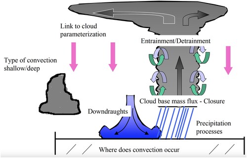
Nowadays all convection schemes used by numerical weather prediction centres are mass flux schemes and so is the IFS scheme which uses the full flux form of the mass flux equations. Such a scheme can be considered as a simplified, but reasonable approximation of the full three-dimensional subgrid convective motions under the assumption of stationarity, the neglect of sub-plume variations and non-hydrostatic pressure forces (Yano et al., 2010; Thuburn et al., 2018). The basic features of the IFS scheme are illustrated in Fig. 12. Shallow or deep convection are represented depending on the cloud depth. If neither of the types can be detected “mid-level”, i.e. local elevated convection is activated when the relative humidity at cloud base exceeds 80% and dynamic lifting is present. The convective drafts consist of a single updraft and downdraft couple that mixes with the environment through detrainment and entrainment. The microphysical processes include mixed phase processes and the generation and fallout of precipitation. Evaporation occurs implicitly through saturated downdrafts and explicitly below cloud base. The convective fluxes are obtained through a rescaling (closure) that for deep convection is based on the convective available energy (CAPE) as introduced by Gregory et al. (2000), while the closure for shallow convection is deduced from the budget of the moist static energy in the sub-cloud layer. The mass flux equations are solved implicitly and the scheme provides convective tendencies for the dry static energy, specific humidity, cloud condensate, rain/snow, momentum and chemical tracers to the IFS. Finally, the link to the prognostic cloud scheme is provided through the detrainment of cloud water/ice that is an important source term and the mass flux subsidence that leads to cloud evaporation. While these basic characteristics are likely rather similar between the different convection schemes used in global models, “details” can have important consequences.

Fig. 12 Schematic of the IFS mass flux convection scheme.

b The Evolution of the IFS Scheme

The evolution of the IFS convection scheme has been driven by the identification of forecast errors at different forecast ranges (e.g. short-range forecast errors in the analysis cycle versus observations or medium-range or seasonal forecast errors versus reanalysis and observations) that can be traced back to the convection scheme.

1 2002/2003 Revised “Trigger Function”

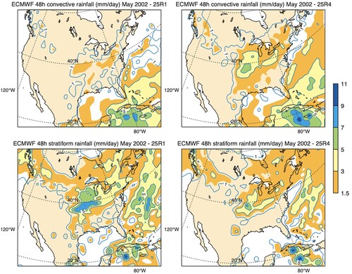
The term trigger function designates a simple procedure to decide on the occurrence of convection and to determine the cloud base properties. The Tiedtke scheme only considered surface based deep convection. Jakob and Siebesma (2003) developed a more realistic sub-cloud model with a strongly entraining parcel departing from the lowest model level. Convection is activated based on the kinetic energy of the parcel at cloud base and the distinction between deep and shallow convection is made depending on a cloud depth threshold of 200 hPa. However, the IFS still strongly underestimated night-time convection over land and instead produced strong grid-scale precipitation, notably during the spring convective season over the continental USA, when the forecasts for Europe were also badly affected by downstream propagating errors. Bechtold et al. (2004) then revised the convective trigger computing convective ascents departing from all model levels below 350 hPa and retaining the first parcel ascent that produces deep convection. As illustrated in Fig. 13 for May 2002 this strongly increased the (night-time) convective precipitation that occurs over the central Great Plains and strongly decreased the excessive grid-scale precipitation, total precipitation is also decreased and in better agreement with observations. Rodwell et al. (2013) concluded that an improved representation of convection over the USA results in improved forecast performance over Europe by strongly reducing the number of bad forecasts. These forecast busts predominantly occur, when there is a strong interaction of convective outflows with the jet stream.

Fig. 13 24–48 h convective and stratiform rainfall (mm day⁻¹) over North America for May 2002 with the operational IFS in 2002 (left column) and with the revised convective initiation allowing convection to depart from any model layer below 350 hPa (right column). This version became operational in 2003.

2 2007 Entrainment, Closure, Numerics

The physics changes in 2007 had probably the largest impact on the tropical forecast performance of the IFS in terms of variability, rainfall distribution and climatology in the last decade. Changes to the shortwave radiation scheme (Morcrette et al., 2008) led to increased convective precipitation over tropical land, while the convection scheme was largely revised as described in Bechtold et al. (2008): the entrainment formulation, consisting of a weak turbulent entrainment and a contribution from moisture convergence was replaced by a relative humidity dependent strong entrainment profile decreasing with height from cloud base values of O (1 km⁻¹) in agreement with large eddy simulations, the detrainment also became relative humidity dependent. Furthermore, the convective adjustment time-scale was no longer constant but computed as the convective turnover time. Finally, an implicit formulation was used to solve for the convective tendencies allowing for large mass fluxes.

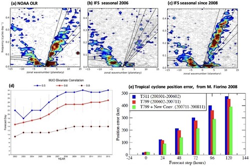
The overall impact of these changes is summarized in Fig. 14. The changes in tropical variability are highlighted by the classical wavenumber frequency spectra of the outgoing longwave radiation (OLR) in the tropical band. While the satellite data display the characteristic equatorially symmetric Kelvin, Rossby and MJO spectral signatures in Fig. 14a, these are very weak in the IFS operational model until November 2007 (Fig. 14b) and in particular the Kelvin wave mode is absent. In contrast, with the revised convection (Fig. 14c) the IFS realistically predicts the main modes of tropical variability. The large-scale tropical precipitation pattern also improved, implying a weaker Hadley cell (less precipitation at the equator) and a more intense Walker cell. Furthermore, the prediction-range of the Madden-Julian oscillation is also strongly increased (Fig. 14d) from about 18 days in 2006 to 24 days in 2008, now in 2020 it is around 30 days (not shown). More on the prediction of the MJO and its teleconnections can be found in Vitart and Molteni (2010). Finally, the prediction of tropical cyclones also strongly improved as the background flow improved, with a reduction in cyclone track error (green bars in Fig. 14e) that comparably is larger than the error reduction obtained by the resolution increase from 40 km in 2005 to 25 km in 2007 (blue and red bars in Fig. 14e).

Fig. 14 Wavenumber frequency spectra of the outgoing longwave radiation from NOAA data (a) and from multi-year integrations with the IFS using the operational cycle in 2006 (b) and with the version that became operational in 2008 (c); the MJO spectral band is highlighted by the black rectangle. (d)–(e) measure the gain in prediction skill: (d) evolution of the prediction skill of the IFS for the MJO between 2002 and 2013 as given by the bivariate correlation with the observed empirical orthogonal functions for wind and outgoing longwave radiation, a value of 0.6 (red line) delimits skillfull forecasts (Vitart & Molteni, 2010), (e) statistics of cyclone positions errors (km) as a function of forecast lead time from the 40 km resolution forecasts in 2005/6 (blue), the 25 km forecasts in 2006/7 (red) and the 25 km forecasts in 2008 (green).

3 2013 Diurnal Cycle

Representing the diurnal cycle of convection over land has been and still is an important and difficult challenge for convection parametrization and even convection permitting models. Resolving the diurnal cycle likely requires convection resolving simulations at 1 km resolution (e.g. Lean et al., 2008). A lot of efforts on this subject have also gone into the IFS. Bechtold et al. (2014) discussed the limits of the convective parcel method and proposed a revised convective closure, where only the fraction of the surface heating/CAPE is released to the free troposphere that does not contribute to boundary-layer mixing. As displayed in Fig. 15 for summer 2012, the revised closure produces a more realistic diurnal cycle of precipitation as a function of local solar time (red line in Fig. 15) compared to radar observations (black line) than the default IFS model before 2013 (sky blue lines) which peaks around noon. The revised scheme was able to shift the convection (CAPE) from a maximum at local noon, coinciding with the maximum in the surface heat fluxes, to a maximum in the late afternoon. However, as also evident in Fig. 15, even with the revised closure there is still a substantial underestimation of convection during night-time in the IFS which is related to difficulties in representing propagating mesoscale convective systems.

Fig. 15 Composite diurnal cycle of precipitation (mm day⁻¹) during JJA 2013 over Europe and continental United States from radar observations (black) and from 24 to 48 h reforecasts with the IFS operational cycle in 2012 (sky blue) and the operational cycle in 2013 (red).

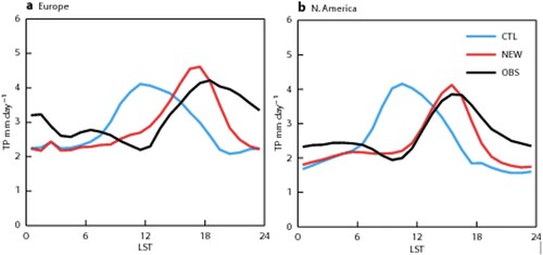
In summary, improvements in the diurnal cycle resulted in better forecasts in regions where the convection and the mean flow are diurnal cycle driven, like the Sahel region of Africa. The quality of the 4-dimensional variational analysis and therefore the initial conditions also benefit from improvements in the diurnal cycle of the model through a better assimilation of time-dependent satellite and conventional data. However, the overall medium-range range forecast performance is only moderately improved by shifts in the diurnal cycle as long as the amplitude, i.e. the total convective heating profile is not altered.

4 2017/2018 Mixed Phase Microphysics

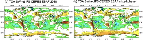
Finally, the last major operational upgrade so far targeted the improvement in convective heating/cooling rates in the upper troposphere and near the melting levels, as well as a reduction in the shortwave radiation errors. Biases in the shortwave radiation penalize both the assimilation of satellite data and the coupled seasonal predictions via the feedback from the sea surface temperatures.

Further improvements in the convective heating rates and the distribution of liquid/ice clouds became possible through: revised mixed phase microphysics, including the glaciation of rain and cloud water in the updraft throughout a revised temperature interval, melting that occurs at the wet bulb temperature, detrainment of the liquid condensate phase only for shallow convection and adding the detrainment of convective rain and snow to the prognostic cloud scheme. The impact of all these changes in terms of annual mean shortwave radiation errors at the top of the atmosphere versus the CERES-EBAF satellite product is shown in Fig. 16. Here we compare annual mean bias from multi-year integrations with the model cycle operational in 2019 (Fig. 16a) and with the same model version, but all ice phase microphysical changes to the convection that have been added between 2017 and 2019 reverted (Fig. 16b). Regions that are particularly affected by the model upgrade are the southern hemisphere storm tracks and to a lesser extent the northern hemisphere storm tracks which all become more reflective through an increase/decrease of the liquid/ice phase in the upper part of the shallow and congestus clouds. Temperature/wind in the upper troposphere and temperatures near the melting level now also better match radiosonde observations (not shown).

Fig. 16 Cloud and radiation evaluation from multi-annual coupled integrations with the IFS Cy47r1. (a)–(b) difference in top of atmosphere net shortwave radiation (W/m²) between the model and the Earth’s Radiant Energy System (CERES) Energy Balanced and Filled (EBAF) product for (a) the operational model version in 2018 and (b) as (a) but with all the changes relating to the mixed phase microphysics added during 2016–2018 removed.

c Mesoscale Convective Systems and Challenges at High Resolution

The lack of night-time convection over land has already been discussed in the context of the diurnal cycle of convection. Today we consider this as the major error in the IFS forecasts of convective activity. That this error is related to the representation of mesoscale convective systems is shown in Fig. 17 which displays the evolution of convection on 12 August 2017 at 15, 18 and 21 UTC over Central Africa and the Sahel region as observed by the 10.8 μm infrared channel of Metsosat-10 (Fig. 17a–c) and the 3-hourly rain accumulations from the TRMM radar product 3B42 (Fig. 17d–f). Consistently, these observations show mesoscale convective systems, notably those near 15°N that intensify during the afternoon and early night-time hours and propagate westward.

Fig. 17 Evolution of continental convective systems over tropical Africa during 12 September 2017 in 3-hourly slots from 15 to 21 UTC as seen by Meteosat-11 infrared image at 10.9 μ wavelength (a,b,c), as well as 3 hourly accumulated rainfall (mm) from 12 to 15, 15 to 18 and 18 to 21 UTC from the TRMM 3B42 product (d,e,f), from the 4 km IFS reforecasts with (g,h,i) (operational version) and without (j,k,l) the deep convection scheme, and with the revised deep convective closure (m,n,o). The IFS reforecasts start at 11 September 2017 at 00 UTC and use the model cycle operational in 2019. There is no TRMM 3B42 data East of 25°E at 21 UTC.

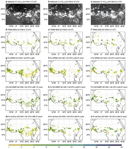
To explore the potential of the IFS at future higher resolutions we have rerun this case with the operational 2019 cycle but at 4 km horizontal resolution with (Fig. 17g–i) and without (Fig. 17j–l) the deep convection parametrisation. As developed through a collaboration with G. Zängl at the DWD (Offenbach) the deep convection scheme includes a smooth reduction of the parametrized convective fluxes (Malardel & Bechtold, 2019), and therefore a transition to resolved convection with increasing resolution (higher than 8 km).

However, with the deep convection parametrisation the rainfall patterns in Fig. 17g–i are too broad scale and the night-time propagating systems at 15°N are absent; similar results are obtained with the operational 9 km horizontal resolution (not shown). In contrast, without the deep convection parametrisation the IFS better simulates the intense westward propagating mesoscale systems. Unfortunately, the amplitude of these systems is too strong as is evident from the comparison with the TRMM data and the global precipitation is overestimated by more than 10%. Also, the root mean square error of precipitation and upper-air forecast skill are significantly degraded with this version of the model.

We therefore further explored the coupling between the convection and the dynamics which is particularly delicate in the case of mesoscale convective systems that propagate and regenerate by producing their own horizontal convergence. Together with Tobias Becker we analysed output from the explicit convection runs over Africa for the whole month of August. It was found that the lack of intense continental convection in the parametrisation can be corrected for by including the vertically integrated advective moisture tendency in the convective instability closure. The results with the revised closure at 4 km are displayed in Fig. 17m–o. Indeed, the convection is now more intense than the current scheme and realistic propagating features develop when compared with the observations in Fig. 17d–f. The revised convective closure now also closely reproduces the satellite observed rainfall distribution (not shown), overall the results are now somewhere in between the current operational scheme with a CAPE closure and the simulations without the deep convection scheme.

Evaluations are ongoing and we plan to implement operationally the above CAPE closure with a moisture convergence term in 2021. As stated in the introduction, we are aiming for a O(5 km) ensemble in 2025–2027 which should also include a revised stochastic physics scheme, namely stochastically perturbed parameters (Leutbecher et al., 2017), where among many parameters from the physical parametrizations, six important parameters of the convection scheme are perturbed. We hope that the ensemble will then be able to largely explore the uncertainties in the predictions and the uncertainties in convection in particular. Ideally, one would aim for a fully prognostic description of convection as has been implemented in a regional model by Gerard (2015). However, such a scheme requires many additional prognostic variables, its closure is not straightforward as is its application in a global model with a 4D-Var data assimilation cycle. There is currently a rapid increase in regional and global applications with explicit deep convection and therefore a fully prognostic convection scheme might eventually never be used in a global model.

IFS operational predictions with explicit deep convection are not likely before 2030, but colleagues (Wedi et al., 2020) are already exploring 1.4 km explicit convection runs of the IFS at the most powerful computer SUMMIT. Preliminary results indicate that the current 9 km model with parametrized convection (effective resolution 30–60 km) and the 1.4 km model give very similar results in terms of spectral energy budget, diurnal cycle etc., with the 1 km model mainly improving scales <100 km. The 9 or 4 km run without deep convection produce however significantly worse results in most aspects including a delayed onset of convection, an overestimation of global precipitation by 5–10% and have difficulties in representing the MJO. Deep convection parametrization seems to remain competitive!

4 The Grell convection scheme

The development of the original Grell convective parameterization began as doctoral work focused on research and science. Since then, the scheme has undergone many transitions, motivated by both research interests and operational constraints. In 1974, Arakawa and Schubert (1974, hereafter AS) and Lord (1978) proposed using a spectrum of updrafts to represent clouds in numerical weather prediction models. Modification of this idealized model served as the basis for the original work that resulted in the Grell scheme. In the first phase of development, the AS scheme was modified to include additional physical processes, most importantly buoyant downdrafts (Grell, 1988). This development was also related to transport of tracers in chemical transport models, where the impact of downdrafts is substantial. Buoyant plumes (positive or negative buoyancy) are very effective transport mechanisms. In a second phase of development (1992–2012), a large effort focused on the simplest and most computationally efficient implementation of convective parameterizations to improve the operational forecasts (Grell, 1993; Grell & Devenyi, 2002; Pan & Wu, 1995). The third phase then focused again on improving the representation of physical processes. This third phase is still ongoing with a resurgent interest from young scientists (Freitas et al., 2021; Grell & Freitas, 2014; Han et al., 2017).

a Modifying and Expanding the Arakawa-Schubert Scheme

As a first step, a parameterization of downdrafts was developed (Grell, 1988) and added to the spectral AS scheme. The downdraft model followed that of an inverted plume (Houze, 1977; Johnson, 1976; Nitta, 1977) driven by the generation of negative buoyant energy, and, therefore, was restricted only to the lower troposphere. The downdraft originating level was assumed to be at the level of minimum moist static energy – in the lowest 300 mb of the atmosphere in the original implementation – to allow the most negatively buoyant downdraft. The original AS parameterization uses a closure that demands a quasi-equilibrium between the “larger scale” and the convection. In AS (1) $\left({\displaystyle \frac{dA}{dt}}\right)={\left({\displaystyle \frac{dA}{dt}}\right)}_{LS}+{\left({\displaystyle \frac{dA}{dt}}\right)}_{CU}\approx 0$(1) where A was defined as the cloud work function, a measure of available buoyancy for a particular cloud type. Subscript $LS$ stands for changes due to the larger scale, subscript $CU$ for changes due to convection. In discretized form this equation became an elegant look (Lord, 1978), but was still complex to solve, since no exact solution existed. Instead, the total change of the cloud work function was minimized using a linear programming method to come to a “quasi” equilibrium. In commonly used applications of the AS scheme, the cloud work function was moved back to climatological values, derived from large observational field campaigns. In Grell-type schemes, Eq. (1) was modified to (2) $\left({\displaystyle \frac{dA}{dt}}\right)={\left({\displaystyle \frac{dA}{dt}}\right)}_{Forc}+{\left({\displaystyle \frac{dA}{dt}}\right)}_{CU}\approx 0.$(2)

In other words, the first term was never perceived as “large” scale, but always as changes to the cloud work function due to impacts from larger scales as well as from other physical processes and the subscript is here replaced by $Forc.$ The most obvious of these physical processes are changes from boundary layer or radiation parameterizations. Later, even changes from convective activity would become part of “Forc”. Additionally, all Grell type schemes – in contrast to the original AS schemes – used forcing functions from the NWP model (large scale advection, PBL parameterization, radiation parameterization) directly to calculate the forcing term. A detailed description of the implementation of the scheme can be found in Grell (1988) and Grell (1993). This version of the parameterization was tested extensively and compared to other parameterizations (Kreitzberg & Perkey, 1976; Krishnamurthi et al., 1980) semi-prognostically using data from the severe midlatitude convective storms field experiment observed during SESAME 1979 (Grell et al., 1991). Additionally, the scheme was tested fully prognostically, again in the mid-latitude severe storm environment, this time with data from the 1985 Pre-STORM experiment (Grell, 1993). The importance of downdrafts was shown for the tests presented in the results. The AS scheme with implemented downdrafts and this application of the “quasi-equilibrium” assumption worked well in the mid-latitude severe storm environment. This included the simulation of a squall line and a mesoscale convective system. A version of the Pennsylvania State University-National Center for Atmospheric Research hydrostatic mesoscale model (MM4; Anthes et al., 1987) was used for this study with 25 km horizontal resolution and 19 vertical levels. To compare to previous studies with a version of the Fritsch and Chappell (1980) scheme (Zhang et al., 1989) the setup was identical to the one chosen by Zhang et al. (1989).

b Improvements Focused on Operational Implementations

Most significant during this time was probably the development of an extremely simple version of the scheme that later was widely used in operations and research and was known as the Grell scheme (hereafter G1). For implementation in operational applications, computational efficiency is essential. In the early 1990s we were looking for a convective parameterization in the Rapid Update Cycle (RUC), which was implemented into operations at the National Center for Environmental Prediction (NCEP) in 1994. The earlier developed version of the AS scheme was too expensive to be used in operations. Hence, the data sets and simulations shown in Grell (1993) were used to simplify the original scheme. The linear programming method solution in the spectral implementation appeared to prefer only a few cloud types. So instead of requiring the quasi-equilibrium, we assumed an equilibrium, and assumed that one cloud type was sufficient to characterize deep convection. Hence (3) ${\left({\displaystyle \frac{dA}{dt}}\right)}_{Forc}=-{\left({\displaystyle \frac{dA}{dt}}\right)}_{CU}$(3) where (4) ${\left({\displaystyle \frac{dA}{dt}}\right)}_{Forc}={\displaystyle \frac{A\left(t+dt\right)-A\left(t\right)}{dt}}$(4) and (5) ${\left({\displaystyle \frac{dA}{dt}}\right)}_{CU}=f\left(CU\right)\ast m_{b\left(CU\right)}$(5) A and f are fairly simple functions in dependence of environmental conditions and assumptions made by the cumulus parameterization. The feedback equations are all normalized by $m_{b\left(CU\right)}$ and can be expressed as (6) ${\displaystyle \frac{\mathrm{\partial }\phi \left(k\right)}{\mathrm{\partial }t}=\varrho \left[\phi \left(z\right)\right]\ast m_{b\left(CU\right)}}$(6) where $\varrho$ is the change of variable $\phi$ per unit of mass. With this simple equation and only one type of cloud allowed, it was realized that the closure is easily changed to other approaches. Stability closures would simply be expressed with (7) ${\displaystyle \frac{A}{\mathrm{\Delta }\tau }=-f\left(CU\right)\ast m_{b\left(CU\right)}}$(7) where $\mathrm{\Delta }\tau$ is some specified time interval over which the instability is removed. Moisture convergence closures were also easy implemented, allowing for direct calculation of the cloud base mass flux, since the total rainfall was related to $m_{b\left(CU\right)}$ with similarly simple equations. Even though the original version of the scheme was oversimplified (no entrainment/detrainment with height), it served as a stepping stone for further developments. At first, different closures were tested and employed for different applications. Giorgi et al. (2012) used the simple scheme in his version of the REGional climate modelling system (REGcm) with different closures.

G1 was also taken by NCEP and modified and implemented as the Simplified Arakawa Schubert (SAS, Pan & Wu, 1995) scheme, of which an improved version is still in operations in various modelling systems at NCEP today. Original modifications by Pan and Wu included simplifying the closure again by assuming that the cloud work function is moved back to a climatological value (as in the original AS approach), but also adding lateral mixing. The SAS scheme went into operation in NCEP’s Global Forecast System (GFS) in 1993. In 2010 the SAS scheme was largely revised by Han and Pan (2011). Some of these revisions were similar to those that were implemented in parallel in Boulder for use in the regional forecast systems (RUC, later the RAP). This included parameterizing the effects of the convection-induced pressure gradient force on convective momentum transport, and the detrainment of cloud condensate into the grid-scale condensate from upper cloud layers above the downdraft initiating level. To deplete more instability in the atmospheric column and result in the suppression of excessive grid-scale precipitation, the scheme was modified to make cumulus convection stronger and deeper by enhancing the maximum allowable cloud base mass flux and by having convective overshooting, respectively.

Another major upgrade for the GFS SAS scheme was made in 2017 (Han et al., 2017). A scale-aware parameterization where the cloud mass flux decreases with increasing grid resolution was developed similar to GF. A simple aerosol-aware parameterization where rain conversion and cloud condensate detrainment in the convective updraft is modified by aerosol concentration number was included. The cloud base mass-flux computation was modified to use convective turnover time as the convective adjustment time scale. The rain conversion rate was modified to decrease with decreasing air temperature above the freezing level, giving rise to more detrainment of cloud condensate in the upper updraft layers and consequently more high clouds. To suppress unrealistically spotty precipitation especially over high terrain during summer time, a convective inhibition in the sub-cloud layer was employed as an additional trigger condition.

In parallel, at NOAA’s Forecast Systems Laboratory (FSL, which is now the Global Systems Laboratory – GSL) the focus for development shifted to the use of different closure assumptions. While all convective parameterizations attempt to statistically represent the interaction between convection and the environment, the closures and assumptions used in individual parameterizations can fundamentally differ. Additionally, some of the parameters used in convective parameterizations are highly sensitive to their assumed value, which can create variability within different iterations of the same convective parameterization (Grell & Devenyi, 2002, GD). While convective parameterizations can be criticized for this variability, GD takes advantage of this diversity. As described above the simple Grell scheme could be used with many different closures, and feedback assumptions were easily changed or modified. Rather than using one set of closures and parameters, GD uses different closures and parameters to create an ensemble. This ensemble is then used to determine the value of cloud base mass flux as well as other feedback properties. The most straightforward and cost-effective approach uses the simple mean of the ensemble. This is the technique that is currently implemented in GD in the Weather and Research Forecast Model (WRF) (Skamarock et al., 2008). GD was implemented into operations in the RUC in 2002.

There are several ways in which GD can be modified so that a more optimal value of cloud base mass flux is selected, since the simple mean is not necessarily the “best” value to choose. For example, a weighted mean of the ensemble members could be calculated. Not only could this weighted mean have different weights assigned to each ensemble member, but those weights could also vary across the domain of the model. Given observational data, techniques such as the linear least squares fitting method, Bayesian data assimilation using probability density function fitting (Grell & Devenyi, 2002), and artificial intelligence could be used to select a better value of cloud base mass flux. Neural networks were also tried to determine better weights with results similar to the least square fitting approach. In a unique approach, the Firefly weighting method proposed by Yang (2008, 2010) was implemented by Dos Santos et al. (2013), based on the bioluminescence process which characterizes firefly mating behaviour. The important aspects that are used in this method by Dos Santos et al. (2013) in determining weights of ensemble members are the light intensity variation and the attractiveness formulation. For simplicity, the attractiveness is determined by the brightness, which in turn is associated with the objective function. For details the reader is referred to Dos Santos et al. (2013).

c Implementing Advanced Physical Processes – for Research and Operations

In parallel to the development of the GD scheme, discussion started about scale-awareness, since horizontal resolution continued to increase in research and operations every year. This led to the development of a three-dimensional application of the GD scheme, which became the G3d parameterization (described also in Grell & Freitas, 2014). The assumption used was that convection, with increased resolution, should impact more than one grid point. Its effects should not be limited to just one grid box, so the parameterization was applied over several grid points (not just one). The ensembles were kept as in GD. G3d became operational in 2012 with the implementation of the first version of the RAPid refresh model (RAPv1).

While the applications of the scheme over neighbouring grid points appeared as the physically most realistic approach, it introduced significant complications, since G3d had to be applied in three dimensions, requiring data communication in parallel applications. Additionally, it was not clear how many grid points would need to be impacted. In parallel, Arakawa et al. (2011) developed an elegant method reobtaining the equation for the vertical eddy transport in terms of the fractional area covered by the active cloud draft and the vertical eddy transport term given by conventional (non-scale aware) tendencies. In that way, the convection parameterization tendencies are simply scaled by a factor that depends on area coverage. Neighbouring grid points are however not impacted. This became one of the foundations of the Grell and Freitas (GF) parameterization, but with many new additional changes and features. This scaling approach is now used in many other convective parameterizations to parameterize scale-awareness, although not all developers claim to follow Arakawa et al. (2011).

GF and G3d scale-aware performance was evaluated many times. Examples are given by Grell and Freitas (2014), Fowler et al. (2016) for variable resolutions, Freitas et al. (2017, 2020, 2021). The paper by Grell and Freitas (2014) showed that the performance of G3d was very similar to GF with respect to scale awareness, but no scaling is applied in G3d. GF used horizontal grid spacings of 20, 10 and 5 km over an area of South America. The full GF scheme (GF-A) was tested on all resolutions and compared to G3d as well as a run without any convection parameterization (NO-CP) and a run with no scale awareness (GF-NS). Each experiment included 15 runs from January 1 to January 15 for 36-hour forecasts, all starting at 00UTC.

When averaged over the domain, a necessary requirement for successful scale-aware applications can usually be seen when comparing resolved versus non-resolved precipitation. This is shown in Fig. 18. With an increase in resolution the precipitation transits from mostly generated by non-resolved to mostly generated by resolved processes (explicit microphysics). In the experiment GF-NS, the parameterized precipitation is much larger than the resolved one, even for a grid spacing of 5 km. Also, the G3d scheme shows a similar ratio to the GF-A formulation.

Fig. 18 Fraction of the resolved precipitation compared to the total precipitation. The 6-hourly model areal mean precipitation rates are averaged for each experiment over the 15 runs.

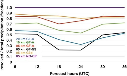
The root mean square error (RMSE) and mean error (Bias) of the precipitation forecasts for the same experiments are seen in Fig. 19. The observed 6-hourly rainfall data were collected at 861 rain-gauge stations distributed over South America. For GF-A on 20, 10, and 5 km horizontal resolutions the daily mean values for RMSE and Bias (in mm/6hr) are (1.85, 0.45), (1.80, 0.32) and (1.81, 0.12), respectively. G3d has very similar performance with daily mean RMSE and Bias of 1.83 and 0.09 mm/6hr, respectively. Turning off the convective parameterization on 5 km (NO CP) leads to a mean Bias of −0.15 mm/6hr and increases the RMSE to 1.98 mm/6hr; larger than the errors of the 10 and 20 km experiments. The GF-NS showed to the worst performance, with a much higher RMSE and Bias.

Fig. 19 As in Fig. 18 except for Root Mean Square Error (RMSE) and mean error (Bias). Units are mm/6hr.

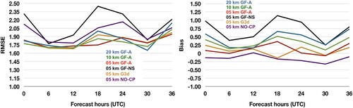
While many other authors also showed impressive performance of this Arakawa et al. (2011) approach as well as other scaling approaches – it was also adapted in the SAS scheme (described above in Section 4.2) – GF never was implemented into the operational storm-scale modelling system, since not only the success but also the flaws of the Arakawa approach became much more visible for storm scale evaluation metrics. Although its application led to improved bias and other commonly used precipitation scores in evaluations, storm-scale verification also depends on realism of precipitation distribution and simulated radar reflectivities. Physically the scaling remains somewhat unrealistic, and this is seen particularly in areas with relatively weak forcing. An example is given in Fig. 20 which shows observed and simulated precipitation over the South East US, using the operational HRRR model with and without the GF scheme, as it was implemented in December of 2020. The scaling leads to wide spread lighter precipitation over Georgia and Alabama. Using no parameterization on the other hand – will lead to a low bias for light precipitation and an over-forecast for large thresholds (Fig. 21). Through tuning (GF employs a threshold when the parameterized clouds are assumed to shrink in size) the bias can be brought in much closer agreement to observation, but the hourly comparison to radar become very unrealistic. Work is now ongoing (see the last section) to bring some of the three dimensionality of G3d back into the GF scheme.

Fig. 20 6hr precipitation forecasts from the HRRR (middle and right panel) for runs without convective parameterizations (middle) and runs with the GF scheme (right panel), compared to observations (right panel) for the same period.

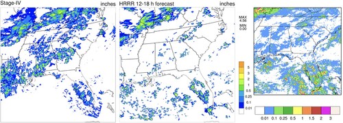
Fig. 21 Frequency BIAS ration for 12hr accumulated precip, August 8–9, a HRRR run without convective parameterizations (blue) and with a version of the GF scheme (red) in dependence of threshold precipitation amounts over the 12 h period ending on August 9, 00z.

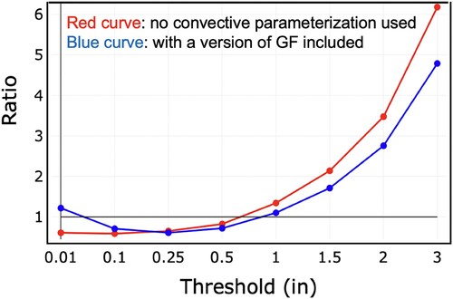
Even more foundational in GF were 2 other changes. (1) The uni-modal approach was replaced with a tri-modal formulation, which allows the three convective modes to exist (Johnson et al., 1999): shallow, congestus, and deep convection. In this unique approach, each of the modes is distinguished by an assumed average size (with a characteristic initial entrainment rate) that strongly controls its vertical depth and profile. (2) While many convective parameterizations use assumptions on entrainment and detrainment to derive a vertical mass flux profile, this was changed in GF by introducing a PDF approach. A characteristic PDF for deep convection is assumed to characterize the vertical mass flux profiles by deep convection in the grid box, and then entrainment and detrainment rates are derived from the vertical mass flux profiles. For deep convection, the maximum of the PDF is given by the stability minimum. For shallow convection, the maximum is just at or above cloud base. Figure 22 shows an example of deep convective mass flux in comparison to observations during the TWP-ICE field experiment. While the closure for deep convection was still using the original ensemble idea from GD, a set of different approaches were introduced to adequately account for the diverse shallow and congestus regimes of convection in a given grid cell. The three modes all transport momentum, tracers, water, and moist static energy. GF also changed the microphysics though inclusion of mixed-phase impacts on buoyancy in the parameterized clouds.

Fig. 22 A Comparison of deep, congestus (mid), and shallow convection massflux profiles for Single Column Model simulations (left) and radar observations (right) during the TWP-ICE field experiment. Observations are from Kumar et al. (2015) showing mass flux profiles derived from windprofilers (black) and CPOL data (red).

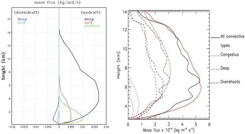
Another new feature is the inclusion of a diurnal cycle closure adapted from Bechtold et al. (2014), which notably improved the simulation of the diurnal cycle of convection and precipitation in Single Column Approaches as well as NASA’s GEOS modelling system (Freitas et al., 2018). Figure 23 compares the net grid-scale vertical moistening (left panels) and heating (right panels) tendencies associated with the three convective modes with (B and D) and without (A and C) the Bechtold closure and for a time dependent SCM run from January to 25 February 1999. Without applying the diurnal cycle closure, the three convective modes coexist and are triggered just a few hours after the sunrise, with the deep convection occurring three to six hours too early, producing a maximum of precipitation about 15 UTC (approximately ∼ 11h local time).

Fig. 23 The time average of the diurnal cycle of the grid-scale vertical moistening (panels A and B) and heating (panels C and D) tendencies associated with the three parameterized convective modes (shaded). The total precipitation and the GF parameterized precipitation from the deep and congestus plumes are shown by the graphic lines: black, green, and purple, respectively. The upper rows show model results without Bechtold’s closure, while in the lower row, this closure is applied (see text for further details).

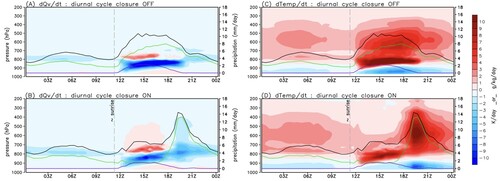
Including the closure (Panels B and D), a smooth and realistic transition is simulated with a late morning and early afternoon low/mid tropospheric moistening by shallow and congestus plumes, followed by a late afternoon and early evening tropospheric drying by the rainfall from the deep cumulus. In this case, the precipitation from the deep penetrative convection is delayed (green contour) with the maximum rate taking place between 18 and 21 UTC, more consistent with the observations of the diurnal cycle over the Amazon region.

d Ongoing and Future Work

Aspects of GF that continue to be actively developed include the treatment of aerosols, inclusion of memory effects, improving microphysics in the parameterized clouds, cold pool generation and movement, and stochastic approaches, as well as further improvements of the scale-awareness (described above). As one implementation of memory effects the parameterization for aerosol wet scavenging has been revised and made proportional to the precipitation efficiency based on Wang et al. (2013). Aerosols in GF can also now be initialized using aerosol optical depth data that varies geographically based on data such as NASA’s Modern-Era Retrospective analysis for Research and Applications, Version 2 (MERRA-2). In the future, for operational applications at NCEP, aerosol optical depth data from NOAA’s global aerosol modelling system could also be used. The coupling of the particle distribution in GF and double moment microphysics parameterizations has also been improved by adding diagnostic estimates of cloud water and cloud ice number concentrations to GF. This modification is designed to diminish the artificial modification of the particle size distribution that occurs when single-moment microphysics from a convective parameterization is used with a double-moment explicit microphysics scheme.

In parallel the SAS scheme is also under continued development. Recently, the scheme was modified to interact with the vertical turbulent mixing scheme in the GFS. Originated from the NCEP SAS scheme in 2010, continuous efforts to improve its performance have been given at the Korea Institute of Atmospheric Prediction Systems (KIAPS). The Korean Integrated Model (KIM) has been operational at the Korea Meteorological Administration (KMA) since April 2020, and a description of the revised SAS scheme in KIM is given in Han et al. (2020).

5 The Zhang-McFarlane convection scheme

The Zhang-McFarlane convection scheme was developed in the early 1990s to replace the moist convective adjustment scheme used in the Canadian Climate Centre General Circulation Model at the time. One of the objectives was to represent convection in a mass flux form so that convective transport could be represented. The paper documenting the scheme and its performance in the model was published a few years later (Zhang & McFarlane, 1995, hereafter ZM scheme). Shortly after, Zhang collaborated with scientists at the National Center for Atmospheric Research (NCAR) and implemented the ZM scheme into the NCAR Community Climate Model version 3 (CCM3) to represent deep convection in the model (Zhang et al., 1998). It has been used since then in subsequent generations of the NCAR model. Over the past quarter century, several modelling centres have also adopted the ZM scheme in their models (Bentsen et al., 2013; Lee et al., 2020; Li et al., 2013; Lin et al., 2020; Xie et al., 2018). Various modifications have also been made to address model simulation deficiencies deemed to be rooted in the parameterization of convection. This section will describe the ZM scheme and its updates.

a The Original Zhang-McFarlane Scheme

The ZM scheme was based on the quasi-equilibrium hypothesis proposed in the classic work of Arakawa and Schubert (1974). It has three main components, the trigger function, a 1-D simplified cloud model and the closure. The trigger function answers the question of whether there will be convection, given the atmospheric conditions. The 1-D cloud model determines the vertical distribution of cloud updraft and downdraft properties and convective heating and drying. The closure determines, in a statistical sense, the amount of convection, often measured in terms of cloud-base convective mass flux.

1 Trigger Conditions

The triggering of convection can depend on many factors. In current convection parameterization schemes, many different convection trigger functions have been used. In the Arakawa and Schubert (1974) scheme a threshold value of cloud work function is used for deep convection trigger. The Tiedtke scheme (Tiedtke, 1989) assumes that convection will be triggered if the atmospheric column has a net moisture convergence and the surface air is buoyant if lifted to the lifting condensation level. In the Kain-Fritsch scheme (Kain, 2004), the trigger function is determined by the vertical velocity and the height of lifting condensation level of parcels lifted from the boundary layer. The convection trigger function in the Donner scheme (Donner, 1993; Donner et al., 2001) requires that the large-scale vertical velocity at the convection initiation level integrated over a time span be able to lift the parcel to the level of free convection (LFC). The Zhang-McFarlane scheme uses a CAPE threshold for convection trigger function. CAPE is defined by (8) $CAPE={\int }_{p_t}^{p_b}{R}_d\left(T_{pv}-T_v\right)d\ln p$(8) where $T_{pv}=T_p\left(1+0.608q_p-q_l\right)$ and ${\overline{T}}_v=\overline{T}\left(1+0.608\overline{q}\right)$ are virtual temperatures of the air parcel and the large-scale mean. p_b and p_t are pressure values at the parcel’s initial level and the neutral buoyancy level, respectively. R_d is gas constant for dry air and q_l is the liquid water condensed following the reversible moist adiabat of the air parcel. The parcel originates at the most unstable layer within the planetary boundary layer. Subscript p stands for the parcel’s properties.

2 The Bulk Cloud Model

The bulk cloud model is based on the idea of entraining plume ensembles, that is, cloud updrafts consist of an ensemble of entraining plumes, each of which has a constant entrainment rate. The plume top is reached when the plume becomes neutrally buoyant. However, instead of determining the cloud properties of each plume individually, the budget equations for the ensemble-mean properties are solved. It is assumed that the plumes are in a steady state. Thus, the budget equations for the updraft ensemble mean are given by (9) ${\displaystyle \frac{\mathrm{\partial }{\eta }_u}{\mathrm{\partial }z}=e_u-d_u}$(9) (10) ${\displaystyle \frac{\mathrm{\partial }{\eta }_u{s}_u}{\mathrm{\partial }z}=e_u\overline{s}-d_u\hat{s}+L\rho c_u}$(10) (11) ${\displaystyle \frac{\mathrm{\partial }{\eta }_u{q}_u}{\mathrm{\partial }z}=e_u\overline{q}-d_u\hat{q}-\rho c_u}$(11) (12) ${\displaystyle \frac{\mathrm{\partial }{\eta }_u{l}_u}{\mathrm{\partial }z}=-d_u{l}_u+\rho c_u-R_u}$(12) where $\eta$ is the cloud mass flux normalized by its value at the cloud base. $e$ and $d$ are normalized entrainment and detrainment rates, respectively. $s=c_{p}T+gz$ is the dry static energy, $q$ is specific humidity, and $l$ is cloud liquid water content. Subscript u denotes updraft. The overbar denotes large-scale grid mean properties in GCMs. $\hat{s}$ and $\hat{q}$ are detrained s and q from updrafts. $c$ is the rate of condensation and $R$ is the rate of conversion of cloud water to rainwater given by (13) $R_u=c_0{\eta }_u{l}_u$(13) where $c_0$ is the conversion coefficient, set to $5.9\times {10}^{-3}{\mathrm{m}}^{-1}$ for land and $4.5\times {10}^{-2}{\mathrm{m}}^{-1}$ for ocean in the NCAR Community Atmosphere Model (CAM). s and q in Eqs. (10) and (11) are often combined to form the moist static energy equation (14) ${\displaystyle \frac{\mathrm{\partial }{\eta }_u{h}_u}{\mathrm{\partial }z}=e_u\overline{h}-d_u\hat{h}}$(14) where $h=s+Lq$ is moist static energy.

The cloud base is treated the same as the convection initiation level, which is at the level of highest moist static energy in the PBL. The cloud top is set at the neutral buoyancy level for each plume. The detrained air is assumed to have the same virtual temperature as the environment and is saturated. The detrained liquid water is assumed to have the same value as that in the updraft.

The vertical profile of the updraft mass flux is specified through fractional entrainment and detrainment rates. For a cloud type with a constant fractional entrainment rate λ its mass flux varies exponentially with height. Integrating over all possible λ’s that contribute to the mass flux at height z gives: (15) $M_u\left(z\right)={\int }_0^{{\lambda }_D\left(z\right)}{m}_b\left(\lambda \right)\exp \left[\left(\lambda \left(z-z_b\right)\right)\right]d\lambda$(15) where $M_u\left(z\right)$ is the total mass flux at height z and $m_b\left(\lambda \right)$ is the mass flux at the cloud base of the plume with entrainment rate $\lambda$. ${\lambda }_D\left(z\right)$ is the fractional entrainment rate of the updrafts that detrain at height z. It is assumed that ${\lambda }_D\left(z\right)$ decreases monotonically with height. Thus, clouds with $\lambda >{\lambda }_D\left(z\right)$ have no contribution to mass flux at height z. In the Arakawa and Schubert (1974) scheme,$m_b\left(\lambda \right)$ was obtained by applying a closure condition to each cloud type. The ZM introduced a simplifying assumption. Note that the bulk cloud base mass flux, denoted by $M_b$, is given by (16) $M_b={\int }_0^{{\lambda }_0}{m}_b\left(\lambda \right)d\lambda$(16) where λ₀ is the maximum fractional entrainment rate corresponding to the shallowest updraft plume of the bulk cloud. The ZM scheme assumes that the cloud base mass flux for each cloud type is independent of the cloud type. Thus, (17) $m_b\left(\lambda \right)={\displaystyle \frac{M_b}{{\lambda }_0}}$(17)

Substituting Eq. (17) into Eq. (16) and carrying out the integration yield (note that ${\eta }_u={\displaystyle \frac{M_u}{M_b}}$): (18) ${\eta }_u\left(z\right)={\displaystyle \frac{1}{{\lambda }_0\left(z-z_b\right)}\exp \left\{{\lambda }_D\left(z\right)\left(z-z_b\right)-1\right\}}$(18)

To determine ${\lambda }_D\left(z\right)$, consider a cloud type with entrainment rate $\lambda$. The moist static energy h_u of the steady-state updraft satisfies: (19) ${\displaystyle \frac{\mathrm{\partial }{h}_u\left(\lambda \right)}{\mathrm{\partial }z}+\lambda \left(h_u\left(\lambda \right)-\overline{h}\right)=0}$(19) This equation can be solved by iteration to obtain ${\lambda }_D\left(z\right)$ such that the air parcel at height z is neutrally buoyant and saturated. At the cloud base, $h_u$ is the same as the large-scale value ${\overline{h}}_b$. The entrainment and detrainment rates can be determined from ${\eta }_u$ and ${\lambda }_D\left(z\right)$.

$s_u$ and $q_u$ can be determined from $h_u$: (20) $s_u=\overline{s}+{\displaystyle \frac{1}{1+\gamma }\left(h_u-{\overline{h}}^{\ast }\right)}$(20) (21) $q_u={\overline{q}}^{\ast }+{\displaystyle \frac{\gamma }{L\left(1+\gamma \right)}\left(h_u-{\overline{h}}^{\ast }\right)}$(21) where $\gamma \equiv \frac{L}{c_p}\frac{\mathrm{\partial }{q}^{\ast }}{\mathrm{\partial }\overline{T}}$. Once $s_u$ and $q_u$ are determined, $c_u$ can be calculated from (10) and then $l_u$ and $R_u$ can be calculated from (12) and (13).

Saturated downdraft produced by precipitation evaporation is assumed to exist when there is precipitation production in the updraft. It starts at the height of minimum saturation moist static energy. The budget equations for bulk downdrafts are given by (22) ${\displaystyle \frac{\mathrm{\partial }{\eta }_d}{\mathrm{\partial }z}=e_d-d_d}$(22) (23) ${\displaystyle \frac{\mathrm{\partial }{\eta }_d{s}_d}{\mathrm{\partial }z}=e_d\overline{s}-d_d{s}_d+L{e}_d}$(23) (24) ${\displaystyle \frac{\mathrm{\partial }{\eta }_d{q}_d}{\mathrm{\partial }z}=e_d\overline{q}-d_d{q}_d-\rho e_d}$(24) (25) ${\displaystyle \frac{\mathrm{\partial }{\eta }_d{h}_d}{\mathrm{\partial }z}=e_d\overline{h}-d_d{h}_d}$(25) where subscript d denotes downdraft. The downdraft mass flux at the downdraft initiation level is assumed to be proportional to mass flux of updraft.

3 The Closure

The closure assumption is a hypothesis that relates convection to the large-scale or model-resolved-scale processes. The original ZM scheme uses a CAPE-based closure. Since the large-scale temperature and moisture changes in both the cloud layer and the subcloud layer due to convective activity are linearly related to the cloud base mass flux, CAPE change due to convection can be written as (26) ${\left({\displaystyle \frac{\mathrm{\partial }CAPE}{\mathrm{\partial }t}}\right)}_{cu}=-F{M}_b,$(26) where F is the CAPE consumption rate by convection per unit cloud base updraft mass flux. To calculate F, one can prescribe a small value of $M_b$ and compute the CAPE change due to this amount of convection. Then F is obtained by dividing the CAPE change by the prescribed value of $M_b$. Alternatively, note that the rate of CAPE change due to convection can be represented in terms of convective tendencies of temperature and moisture in both the free troposphere and the PBL, which are linearly proportional to $M_b$. One can compute convective CAPE change per unit cloud base mass flux, and thus F and it depends on the large-scale thermodynamic profiles and the cloud model. In the ZM scheme, the latter approach is used.

The closure condition is that the CAPE is removed at an exponential rate by convection with a characteristic adjustment time scale τ: (27) ${\left({\displaystyle \frac{\mathrm{\partial }CAPE}{\mathrm{\partial }t}}\right)}_{cu}=-{\displaystyle \frac{CAPE-CAP{E}_0}{\tau }.}$(27)

Thus (28) $M_b={\displaystyle \frac{CAPE-CAP{E}_0}{\tau F},}$(28) where $\tau$ is the relaxation timescale and is set to 2 h in CAM5. $CAP{E}_0$ is the threshold value of CAPE for triggering convection, and is set to 70 J/kg.

b Revisions to the ZM Scheme

There have been a number of updates to the original ZM scheme. Some are revisions to elements in the original scheme, others are additions to enhance the scheme.

1 Diluted CAPE

The CAPE calculation in the original ZM scheme assumes that the air parcel, when lifted, first follows a dry adiabat, and after reaching the lifting condensation level it follows a pseudo-moist adiabat, with no entrainment dilution. This decouples the tropospheric humidity, particularly in the lower troposphere, from convection. As such, it overestimates the frequency of convection, especially when the lower troposphere is dry. To remedy this, Neale et al. (2008) introduced entrainment dilution into the CAPE calculation. It is assumed that the parcel’s air mass is doubled every kilometre from the entrainment of the environmental air as it rises to the neutral buoyancy level. Because of the dilution, the CAPE values can be very small in dry environment even when the undilute CAPE is large (Zhang, 2009), thereby reducing the frequency of fictitious occurrence of convection.

2 dCAPE-Based Closure

The CAPE-based closure often produces too frequent convection, even with diluted CAPE. In addition, since CAPE is tied too closely to the boundary layer temperature and moisture, which are strongly influenced by surface turbulent fluxes, convection in the GCM often occurs too early during the day, leading to the wrong diurnal cycle (Dai, 2006). Zhang (2002, 2003) examined the relationships between convection and the large-scale thermodynamic fields using field observations from the U.S. DOE Atmospheric Radiation Measurement (ARM) programme at the Southern Great Plains site and the Tropical Ocean–Global Atmosphere Coupled Ocean-Atmosphere Response Experiment (TOGA COARE) intensive observation period in the tropical western Pacific. He found that under both tropical maritime and midlatitude continental conditions, convection is highly correlated with the large-scale generation of CAPE in the free troposphere (referred to as dCAPE), and proposed to use dCAPE as closure. dCAPE was first used by Xie and Zhang (2000) as a trigger condition for convection.

The dCAPE closure is based on the fact that CAPE as defined in Eq. (1) is determined by the difference between the parcel’s virtual temperature and that of its environment. Thus, the time rate of change of CAPE is given by the difference of the vertical integral of the time rate of change of the parcel’s virtual temperature and that of the environment. Observations show that CAPE change with time is dominantly (∼90% or more) governed by contributions of the parcel’s virtual temperature, which for undilute parcels is entirely determined by temperature and moisture changes in the PBL. In other words, the contribution to CAPE change from the free troposphere is negligible compared to that from the PBL, that is, (29) ${\displaystyle \frac{\mathrm{\partial }CAP{E}_{ft}}{\mathrm{\partial }t}=-{\int }_{p_t}^{p_b}{R}_d{\displaystyle \frac{\mathrm{\partial }{\overline{T}}_v}{\mathrm{\partial }t}d\ln p\approx 0}}$(29)

This forms the basis of the dCAPE-based closure. Since the net CAPE change can be represented as the sum of changes due to convection and those due to non-convective (i.e. large-scale) processes, formally Eq. (21) becomes (30) ${\left({\displaystyle \frac{\mathrm{\partial }CAP{E}_{ft}}{\mathrm{\partial }t}}\right)}_{cu}=-{\int }_{p_t}^{p_b}{R}_d{\left({\displaystyle \frac{\mathrm{\partial }{\overline{T}}_v}{\mathrm{\partial }t}}\right)}_{cu}d\ln p=-{\left({\displaystyle \frac{\mathrm{\partial }CAP{E}_{ft}}{\mathrm{\partial }t}}\right)}_{ls}={\int }_{p_t}^{p_b}{R}_d{\left({\displaystyle \frac{\mathrm{\partial }{\overline{T}}_v}{\mathrm{\partial }t}}\right)}_{ls}d\ln p$(30)

This is well supported by ARM observations (Fig. 24) during its summer 1997 field campaign. The x-axis represents ${\left(\frac{\mathrm{\partial }CAP{E}_{ft}}{\mathrm{\partial }t}\right)}_{ls}$ and the y-axis represents ${\displaystyle \frac{\mathrm{\partial }CAP{E}_{ft}}{\mathrm{\partial }t}}$.

Fig. 24 Scatter plot of the CAPE change due to the ambient virtual temperature change vs. CAPE change due to large-scale forcing from advection and radiative cooling during the ARM summer 1997 IOP. Triangles are for convective periods, crosses and dots are for non-convective periods, the latter of which are for CIN < −100 J/kg. From Zhang (2002).

Since ${\left(\frac{\mathrm{\partial }CAP{E}_{ft}}{\mathrm{\partial }t}\right)}_{cu}$ is proportional to cloud base mass flux, we have the final expression for the dCAPE-based closure: (31) $M_b=-{\displaystyle \frac{1}{K}{\int }_{p_t}^{p_b}{R}_d{\left({\displaystyle \frac{\mathrm{\partial }{\overline{T}}_v}{\mathrm{\partial }t}}\right)}_{ls}d\ln p}$(31) where (32) $K={\int }_{p_t}^{p_b}\left[\left(1+0.608\overline{q}\right)\left(-\eta {\displaystyle \frac{\mathrm{\partial }s}{\mathrm{\partial }p}}\right)+0.608\overline{T}\left(-\eta {\displaystyle \frac{\mathrm{\partial }\overline{q}}{\mathrm{\partial }p}+d_u\left(q_s-\overline{q}\right)}\right)\right]d\ln p$(32) is similar to F in Eq. (18) except it is the CAPE consumption rate in the free troposphere per unit cloud base mass flux. The integrand in the equation is nothing but virtual temperature change of the convection environment due to convective heating and drying.

This closure significantly improved the simulation of precipitation in the single column model of the NCAR CCM3 compared to the original ZM scheme (Fig. 25). It also produced a much better simulation of Madden Julian oscillation (Zhang & Mu, 2005) in the NCAR CCM3, as well as reduced the double ITCZ bias in the NCAR CCSM3 (Song & Zhang, 2009; Zhang & Song, 2010; Zhang & Wang, 2006).

Fig. 25 Precipitation time series observed (blue line) during the ARM 1997 IOP at the SGP site and simulated by a single column model using the original ZM scheme (dashed line, top) and the revised ZM scheme with dCAPE closure (dashed line, bottom).

c Addition of New Functionalities

1 Convective Cloud Microphysics

In the ZM scheme the formation of precipitation is treated through a tunable conversion coefficient c₀ in the bulk cloud model (Eq. (13)). To more accurately represent the microphysical processes that are involved in the conversion from cloud water to rainwater, Song and Zhang (2011) developed a 2-moment convective microphysics scheme, which was later incorporated in the ZM scheme in the NCAR CAM3 (Song et al., 2012). Instead of folding all microphysical processes into a single tuning parameter, the scheme explicitly treats mass mixing ratio and number concentration of four hydrometeor species (cloud water, cloud ice, rainwater and snow). The microphysical processes considered include cloud droplet activation, freezing, cloud ice nucleation, autoconversion, self-collection, collection between hydrometeor species, and sedimentation (Fig. 26).

Fig. 26 Schematic showing the microphysical processes represented in the convective microphysics parameterization of the ZM scheme.

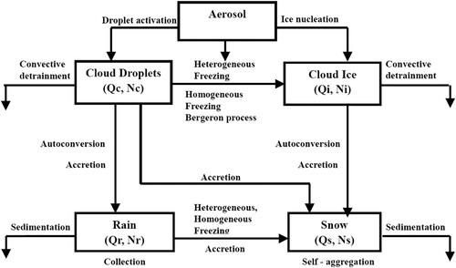
For given convective updraft mass flux (${\eta }_u$) and detrainment rate ($d_u$) from the ZM scheme, the diagnostic budget equations for mass mixing ratio $q_x$ (in units of kg kg⁻¹), and number concentration $N_x$ (in units of kg⁻¹), where the subscript x denotes cloud water, cloud ice, rainwater, or snow in saturated updrafts, can be written as: (33) ${\displaystyle \frac{\mathrm{\partial }{\eta }_u{q}_x}{\mathrm{\partial }z}=-d_u{q}_x+{\sigma }_u{S}_x^q}$(33) (34) ${\displaystyle \frac{\mathrm{\partial }{\eta }_u{N}_x}{\mathrm{\partial }z}=-d_u{N}_x+{\sigma }_u{S}_x^N}$(34) where ${\sigma }_u$ is the fractional area occupied by convective updrafts. $S_x^q$ and $S_x^N$ are the source/sink terms for $q_x$ and $N_x$, respectively, per unit cloud area. They include autoconversion of cloud water/ice to rain/snow; accretion of cloud water by rain; accretion of cloud water, cloud ice, and rain by snow; homogeneous and heterogeneous freezing of cloud water/rain to form ice/snow; Bergeron-Findeisen process; fallout of rain and snow; condensation/deposition; self-collection of rain drops; self-aggregation of snow; activation of cloud condensation nuclei or ice nucleation. Contributions from each of these source/sink terms are parameterized in Song and Zhang (2011). The vertical profiles of hydrometeors within the updrafts are obtained by integrating (33) and (34) from cloud base upward. The detrainment of cloud ice and liquid water (both mass mixing ratio and number concentration) is then added to the grid-scale cloud microphysics scheme.

2 Stochastic Convection

In the ZM scheme, the convective mass flux represents an ensemble mean from a population of convective clouds in a statistical sense. As the model resolution increases, the stochasticity kicks in. To represent the stochasticity in convection, the Plant and Craig (2008) stochastic convection scheme was incorporated into the ZM scheme, such that the probability of the cloud base mass flux is determined by the stochastic scheme while the expected mean of the probability distribution of mass flux in the stochastic scheme is determined by the closure of the ZM scheme. In the stochastic convection scheme, the mass flux of a cloud is assumed to follow an exponential distribution, and thus the average number of clouds having a mass flux between m and m + dm is given by (35) $d\overline{n}\left(m\right)=〈N〉p\left(m\right)dm={\displaystyle \frac{〈N〉}{〈m〉}{e}^{-{\displaystyle \frac{m}{〈m〉}}}dm.}$(35) where $〈N〉$ is the ensemble mean number of clouds and is given by $〈N〉=〈M〉/〈m〉$. $〈M〉$ is the ensemble mean cloud base mass flux and is given by the closure of the ZM scheme, and $〈m〉$ is the mean mass flux of a cloud, which is prescribed as a tuning parameter. The number of clouds with mass flux m follows a Poisson distribution: (36) $p_{N_m}\left(n\right)={\displaystyle \frac{{〈N_m〉}^n{e}^{-〈N_m〉}}{n!}\mathrm{f}\mathrm{o}\mathrm{r}n=0,1,2,\dots }$(36) where $〈N_m〉$ is the average number of clouds with mass flux m. It follows then (37) $p_{d\overline{n}\left(m\right)}\left(n\right)={\displaystyle \frac{d\overline{n}{\left(m\right)}^n{e}^{-d\overline{n}\left(m\right)}}{n!}}$(37)

For small $d\overline{n}\left(m\right)$, (38) $p_{d\overline{n}\left(m\right)}\left(1\right)\approx d\overline{n}\left(m\right)={\displaystyle \frac{〈N〉}{〈m〉}{e}^{-{\displaystyle \frac{m}{〈m〉}}}dm}$(38) and the probability of more than one cloud (i.e. $p_{d\overline{n}\left(m\right)}\left(2\right)$, $p_{d\overline{n}\left(m\right)}\left(3\right)$, …) is of higher order in $d\overline{n}\left(m\right)$ and can be neglected.

A common bias in many GCMs is that light rain occurs too frequently while the frequency of heavy rain occurrence is severely underestimated. The incorporation of stochastic convection into the ZM scheme in the NCAR CAM5 reduced a major bias in the simulated precipitation intensity in the model (Wang et al., 2016). Figure 27 shows an example of such improvements.

Fig. 27 (a) Frequency distributions of precipitation rate and (b) cumulative contribution from each binned precipitation rate based on daily mean precipitation data. The results are for the global belt of 20°S–20°N from the Tropical Rainfall Measurement Mission (TRMM) observation (black line), CTL (blue line) and EXP (red line). From Wang et al. (2016).

6 Parameterization of shallow moist convection

Shallow moist convection, which includes stratus, stratocumulus, and shallow cumulus clouds, exerts a significant impact on the radiative budget of the Earth and strongly affects the vertical transport of enthalpy, moisture, and momentum in the low troposphere. Many problems associated with the simulated variabilities of tropical convection from diurnal to intraseasonal timescales, including a poor simulation of the Madden-Julian Oscillation (MJO) and the diurnal cycle of precipitation over land, are related to the inadequate treatment of sub-grid scale (SGS) processes of shallow moist convection in numerical models (e.g. Grabowski et al., 2006; Hagos et al., 2010). Much of the uncertainty in climate change projections by general circulation models (GCMs) can also be attributed to the parametric treatment of shallow moist convection in the tropics and subtropics (Bony & Dufresne, 2005; Medeiros et al., 2008). To date, a realistic representation of the SGS processes of shallow convection in large-scale models continues to be a challenge. This section reviews how shallow moist convection is parameterized in the state-of-the-art full physics numerical models.

In large-scale models, the shallow cumulus and stratus/stratocumulus are often treated separately by different schemes or modules partially due to the different cloud processes associated with the two types of clouds and partially due to historical reasons. The development of cumulus convection parameterization can be traced back to the pioneer work by Arakawa and Schubert (1974) who constructed the dynamic view of interaction between cumulus and the environment in which the convection is embedded: Down-scaling, the environment controls the convective activities through stabilization/destabilization processes; Up-scaling, cumulus convection alters the thermodynamic structure of the environment through the subsidence induced by the convective updrafts and the detrainment of heat, water vapour, and cloud hydrometers from updrafts. This allowed Arakawa and Schubert (1974) to develop a mass-flux based cumulus scheme by assuming a quasi-equilibrium between the generation of moist convective instability by environmental processes and the stabilizing effect of cumulus convection on the environment. Since then, many convection schemes based on the quasi-equilibrium assumption have been developed. Although these schemes differ in details, they all have three components: (a) a convective cloud model that determines the vertical redistribution of heat, vapour, hydrometeor, and precipitation; (b) an entrainment and detrainment parameterization that describes how the convection interacts with the environment; and (c) a closure at the convection release height that determines when and at what height the convection initiates. Although the quasi-equilibrium assumption and three-component structure were originally proposed for deep convection parameterization, this strategy has been adopted by some sophisticated shallow convection schemes used in GCMs, such as NCAR CAM (Bretherton et al., 2004a), ECMWF (Kohler et al., 2011; Soares et al., 2004) and Météo France (Pergaud et al., 2009).

The most commonly used cloud model in convection schemes is developed under the mass-flux framework in which the kinematic vertical flux of a generic variable $\psi$ is decomposed into four parts following a top-hat distribution, (39) $\overline{w^{\mathrm{\prime }}{\psi }^{\mathrm{\prime }}}=\sigma {\overline{w^{\mathrm{\prime }}{\psi }^{\mathrm{\prime }}}}^u+\left(1-\sigma \right){\overline{w^{\mathrm{\prime }}{\psi }^{\mathrm{\prime }}}}^e+\sigma \left({\overline{w}}^u-\overline{w}\right)\left({\overline{\psi }}^u-\overline{\psi }\right)+\left(1-\sigma \right)\left({\overline{w}}^e-\overline{w}\right)\left({\overline{\psi }}^e-\overline{\psi }\right)$(39) where $w$ is the vertical velocity, overbar and overbar indexed with superscripts u and e indicate the averages over an area, positively buoyant updraft of convection in the area, and environment in which the convective updraft is embedded, respectively, and $\sigma$ is the fraction of convective updraft of the area. The first and second terms on the right-hand side (RHS) of Eq. (39) represent the fluxes induced by the turbulence within the updraft and environment, respectively. The sum of the third and fourth terms on the RHS of Eq. (39) represents the fluxes induced by the coherent updrafts and the associated environment. Assuming that a generic variable also follows the same top-hat distribution, the mean of the variable may be decomposed as $\overline{\psi }=\sigma {\overline{\psi }}^u+\left(1-\sigma \right){\overline{\psi }}^e$, then, the sum of the third and fourth terms on the RHS of Eq. (39) may be rewritten as, (40) ${\overline{w^{\mathrm{\prime }}{\psi }^{\mathrm{\prime }}}}^u=\sigma \left(1-\sigma \right)\left({\overline{w}}^u-{\overline{w}}^e\right)\left({\overline{\psi }}^u-{\overline{\psi }}^e\right)=M_u\left({\overline{\psi }}^u-{\overline{\psi }}^e\right),$(40) where ${\overline{w^{\mathrm{\prime }}{\psi }^{\mathrm{\prime }}}}^u$ is the kinematic vertical flux induced by the coherent features associated with the updraft and environment, and $M_u=\sigma \left(1-\sigma \right)\left({\overline{w}}^u-{\overline{w}}^e\right)$ is known as the kinematic updraft mass flux. The transport induced by the turbulence within the updraft and environment may be appropriately described by local mixing mechanism. Thus, in numerical simulations the vertical fluxes represented by the first and second terms on the RHS of (39) are often handled by a turbulent mixing scheme that also parameterizes the turbulence in the planetary boundary layer (PBL). In contrast, the mixing induced by convection is fundamentally non-local. Thus, a convection scheme is specifically designed to account for the non-local transport represented by ${\overline{w^{\mathrm{\prime }}{\psi }^{\mathrm{\prime }}}}^u$. Note that not all cumulus clouds are positively buoyant. For shallow convection, the negatively buoyant cumulus can be up to 40% according to observations (Taylor & Baker, 1991) and large eddy simulations (LESs, Siebesma & Cuijpers, 1995; Zhu & Albrecht, 2003). Nonetheless, Siebesma and Cuijpers (1995), Wang and Stevens (2000), and Zhu (2015) showed that the coherent updrafts account for 80–90% of the total fluxes in the shallow cumulus layer, indicating that the decomposition of total flux in an area in terms of the positively buoyant updraft is appropriate for parameterizing the vertical transport induced by shallow cumulus convection. In real practice, since cloud fraction $\sigma$ is usually smaller than 20% for shallow cumulus (Siebesma & Cuijpers, 1995), Eq. (40) is often simplified as, (41) ${\overline{w^{\mathrm{\prime }}{\psi }^{\mathrm{\prime }}}}^u\approx \sigma {\overline{w}}^u\left({\overline{\psi }}^u-\overline{\psi }\right)=M_u\left({\overline{\psi }}^u-\overline{\psi }\right),$(41) where it assumes ${\overline{\psi }}^e\approx \overline{\psi }$, ${\overline{w}}^e\approx \overline{w}\approx 0$, and $\sigma \ll 1$. From Eq. (3), it is clear to calculate the cumulus induced vertical fluxes, updraft mass flux $M_u$ and mean updraft property ${\overline{\psi }}^u$ need to be determined. From the conservation law,$M_u$ and ${\overline{\psi }}^u$ should obey the mass continuity equation and dilution equation, respectively (Betts, 1973), (42) ${\displaystyle \frac{\mathrm{\partial }{M}_u}{\mathrm{\partial }z}=E-D,}$(42) (43) ${\displaystyle \frac{\mathrm{\partial }\left(M_u{\overline{\psi }}^u\right)}{\mathrm{\partial }z}=E\overline{\psi }-D{\overline{\psi }}^u,}$(43) where $E$ and $D$ are the lateral entrainment and detrainment mass flux per unit height. Defining $ϵ$ and $\delta$ as the fractional entrainment and detrainment rate, (44) $E=ϵM_u,D=\delta M_u.$(44)

Inserting Eq. (44) into (42) and (43), it yields, (45) ${\displaystyle \frac{1}{M_u}{\displaystyle \frac{\mathrm{\partial }{M}_u}{\mathrm{\partial }z}=ϵ-\delta ,}}$(45) (46) ${\displaystyle \frac{\mathrm{\partial }{\overline{\psi }}^u}{\mathrm{\partial }z}=ϵ\left(\overline{\psi }-{\overline{\psi }}^u\right).}$(46)

Eq. (46) indicates that the change of updraft property is solely caused by entraining environmental air into the updraft.

The cloud model described by (45) and (46) is not closed. To solve the equations, $ϵ$ and $\delta$ need to be determined. For shallow cumulus convection, both observations from the Barbados Oceanographic and Meteorological Experiment (BOMEX, Esbensen, 1978) and LES (Siebesma & Cuijpers, 1995) show that the entrainment and detrainment rate decreases with height from cloud base to cloud top. One of the methods to parametrically determine $ϵ$ and $\delta$ is the buoyancy sorting approach proposed by Kain and Fritsch (1990) and Bretherton et al. (2004a). It assumes that over a small increment of depth $\delta z$ in the cloud layer, equal parts of updraft and environmental air mass flux ${\eta }_0{M}_u\delta z$ are mixed up laterally, where ${\eta }_0$ refers to a fraction of updraft and environmental air close to the cloud edge that is involved in the lateral mixing. The total mixing mass flux is, therefore, $2{\eta }_0{M}_u\delta z$. But the mixing creates a spectrum of mixtures. Some of the mixtures continue to be positively buoyant and keep rising, but the rest becomes negatively buoyant and detrains from the updraft. Thus, to describe the status of a mixture, one may define a fraction index $\chi$ ranging from 0 for the undiluted updraft to 1 for pure environmental air. The probability distribution function (PDF) of a certain mixture with $\chi$ may be described by $\xi \left(\chi \right)$. For all mixtures, there should exist a critical ${\chi }_c$. Mixtures with $\chi <{\chi }_c$ will remain positively buoyant and those with $\chi \ge {\chi }_c$ will be neutral or negatively buoyant. For a certain ${\chi }_c$, the net change of updraft mass flux $\delta M_u$ over a depth $\delta z$will be, (47) $\begin{array}{rl}\delta M_u=& {\int }_0^{{\chi }_c}2{\eta }_0{M}_u\delta z\chi \xi \left(\chi \right)d\chi -{\int }_{{\chi }_c}^{1}2{\eta }_0{M}_u\delta z\left(1-\chi \right)\xi \left(\chi \right)d\chi \\ =& {\eta }_0{M}_u\delta z{\chi }_c^2-{\eta }_0{M}_u\delta z(1-{\chi }_c{)}^2.\end{array}$(47)

The first and second term in Eq. (47) represent the environmental air entrained in the updraft and updraft air detrained in the environment, respectively. Note that to calculate the integrations in Eq. (47), the PDF $\xi \left(\chi \right)$ has been assumed to follow a uniform distribution, i.e. $\xi \left(\chi \right)=1$, (Bretherton et al. 2004). As $\delta z\to 0$, Eq. (47) becomes, (48) ${\displaystyle \frac{1}{M_u}{\displaystyle \frac{\mathrm{\partial }{M}_u}{\mathrm{\partial }z}={\eta }_0{\chi }_c^2-{\eta }_0(1-{\chi }_c{)}^2=ϵ-\delta ={\eta }_0(2{\chi }_c-1).}}$(48)

For a different PDF function $\xi \left(\chi \right)$, the integration of Eq. (47) will be different and will involve complicated calculations. But as pointed out by Bretherton et al. (2004), no observational evidence is available to show the preference of a specific PDF function to others. Thus, for simplicity here we choose the uniform distribution. From (48), it is clear that the entrainment and detrainment rate in a buoyancy sorting model is determined by the fraction of updraft and environmental air involved with the lateral mixing ${\eta }_0$ and the critical mixture index ${\chi }_c$ that makes the mixture buoyant with respect to the environment. Kain and Fritsch (1990) related ${\eta }_0$ to the inverse of the updraft diameter $R^{-1}$. Bretherton et al. (2004) further scaled $R$ to the height of cumulus convection to obtain ${\eta }_0=\frac{c_0}{H}$, where $c_0$ is am empirical coefficient taken as 15 according to the best estimate from LESs, $H$ is the height of cumulus from the previous model time step.

${\chi }_c$ may be estimated from a linear combination of the updraft and environment following Randall (1980) and Deardorff (1980)’s method. Defining liquid water potential temperature as ${\theta }_l=\theta -{\displaystyle \frac{L\theta }{C_{p}T}{q}_l}$ and total water mixing ratio as $q_t=q_v+q_l$, where $T$ is the temperature; $\theta$ is the potential temperature; $q_v$ and $q_l$ are the mixing ratio of water vapour and liquid water; $L$ is the specific latent heat of vaporization; and $C_p$ is the specific heat of dry air at constant pressure. Let $m_u$, ${\theta }_{lu}$, $q_{tu}$, $m_e$, ${\theta }_{le}$, and $q_{te}$ be mass, liquid water potential temperature, and total water mixing ratio of the updraft and environment, respectively. Not that the environment air is unsaturated, thus, ${\theta }_{le}={\theta }_e$ and $q_{te}=q_{ve}$. The liquid water potential temperature and total water mixing ratio of a mixture will be, (49) ${\theta }_{lf}=\left(1-\chi \right){\theta }_{lu}+\chi {\theta }_{le},$(49) (50) $q_{tf}=\left(1-\chi \right)q_{tu}+\chi q_{te},$(50) where $\chi =\frac{m_e}{m_u+m_e}$ is the mixing fraction index with 0 being undiluted updraft and 1 being pure environmental air, and subscript “$f$” indicates the mixture. Now we want to find ${\chi }_s$ so that the mixture is just saturated mixture, i.e. (51) $q_{tf}=q_{sf}\left({\theta }_{lf}\right)=q_{sf}\left[{\theta }_{lu}+{\chi }_s\left({\theta }_{le}-{\theta }_{lu}\right)\right],$(51) where $q_{sf}\left({\theta }_{lf}\right)$ is the saturated mixing ratio of the mixture at ${\theta }_{lf}$. Since $\left({\theta }_{le}-{\theta }_{lu}\right)\ll {\theta }_{lu}$, Eq. (51) may be expanded as the Taylor series. Taking terms of O(${\theta }_{le}-{\theta }_{lu}$), it yields, (52) $q_{tf}=q_{sf}=q_s\left({\theta }_{lu}\right)+{\chi }_s{\displaystyle \frac{\mathrm{\partial }{q}_s}{\mathrm{\partial }{\theta }_l}\left({\theta }_{le}-{\theta }_{lu}\right).}$(52)

Within the range of $[{\theta }_{le},{\theta }_{lu}]$, ${\displaystyle \frac{\mathrm{\partial }{q}_s}{\mathrm{\partial }{\theta }_l}}$ is nearly a constant, thus, Eq. (52) may be rewritten as, (53) $q_{tf}=q_{sf}=q_s\left({\theta }_{lu}\right)+{\chi }_s\left[q_s\left({\theta }_{le}\right)-q_s\left({\theta }_{lu}\right)\right].$(53)

Combining Eq. (15) with Eq. (50), one obtains, (54) ${\chi }_s={\displaystyle \frac{q_{tu}-q_s\left({\theta }_{lu}\right)}{\left[q_{tu}-q_{te}\right]-\left[q_s\left({\theta }_{lu}\right)-q_s\left({\theta }_{le}\right)\right]}.}$(54)

For the mixture that is just buoyant with respect to the environment, one needs to find, (55) ${\theta }_{vf}={\theta }_{ve},$(55) where ${\theta }_{vf}={\theta }_f\left[1+ϵq_{sf}-\left(q_{tf}-q_{sf}\right)\right]$ is the virtual potential temperature of the mixture, $ϵ=R_d/R_v$ is the ratio of gas constant of dry air to water vapour, ${\theta }_{ve}$ is the virtual potential temperature of the environment. ${\theta }_f$ may be expressed as ${\theta }_f={\theta }_{lf}+\pi {\displaystyle \frac{L}{C_p}\left[q_{tf}-q_{sf}\right]}$, where $\pi ={\displaystyle \frac{\theta }{T}={\left({\displaystyle \frac{p_0}{p}}\right)}^{\left(R_d/C_p\right)}}$, $p_0$ is a reference pressure, then, one can theoretically find a ${\chi }_c$ that makes the mixture just buoyant with respect to the environment by solving Eq. (55), but it is not a trivial mathematical problem. In practice, one may utilize the approximate linear relationship among ${\theta }_{vf}$, ${\theta }_{vu}$, and ${\theta }_{ve}$ to provide a good estimate of ${\chi }_c$ as illustrated by Fig. 28, (56) ${\chi }_c={\chi }_s\left(1-{\displaystyle \frac{{\theta }_{ve}-{\theta }_{vfs}}{{\theta }_{vu}-{\theta }_{vfs}}}\right).$(56)

Fig. 28 Virtual potential temperatures for fractional mixtures of updraft and environmental air, where ${\chi }_s$ and ${\chi }_c$ denote the fraction where the mixture is just saturated and just buoyant with respect to the environment. ${\theta }_{vfs}$ is the virtual potential temperature of the mixture that is just saturated.

With an appropriate parameterization of entrainment and detrainment rate, the convection system described by (45) and (46) now can be closed by providing the low boundary conditions at the cumulus base. It describes how convection is initiated. The cloud base may be naturally defined at the lifting condensation level (LCL). However, not all plumes that reach LCL can overcome the convection inhibition (CIN) so that they can develop freely due to their buoyancy. Only those plumes at the cloud base (or LCL) that have vertical velocities greater than a critical value, $w>w_c$, can penetrate the CIN and reach the level of free convection (LFC), from there, they may develop into positively buoyant updrafts. From energy balance perspective, $w_c$ is determined by CIN as, $w_c=\sqrt{2aCIN}$, where $a$ is the virtual mass coefficient, usually taken as $a=1$ (Simpson & Wiggert, 1969), and CIN, following its definition, may be calculate as the enclosed area by the vertical profiles of virtual potential temperature of the environment and an air parcel that undergoes an adiabatic process.

The vertical velocity at the cloud base may be estimated by assuming that the distribution of $w$ follows a Gaussian function, (57) $f\left(w\right)={\displaystyle \frac{1}{\sqrt{2\pi \overline{w^{{}^{\mathrm{\prime }}2}}}}\mathrm{e}\mathrm{x}\mathrm{p}\left(-{\displaystyle \frac{w^2}{2\overline{w^{{}^{\mathrm{\prime }}2}}}}\right),}$(57) where $\overline{w^{{}^{\mathrm{\prime }}2}}$ is the vertical velocity variance. The fraction of updraft and kinetic updraft mass flux at the cloud base are the integration of$f\left(w\right)$ and $wf\left(w\right)$ from $w_c$ to infinity, respectively, (58) ${\sigma }_{cbs}={\int }_{w_c}^{\mathrm{\infty }}f\left(w\right)dw={\displaystyle \frac{1}{2}\mathrm{e}\mathrm{r}\mathrm{f}\mathrm{c}\left({\displaystyle \frac{w_c}{\sqrt{2\overline{w^{{}^{\mathrm{\prime }}2}}}}}\right),}$(58) (59) $M_{u,cbs}={\int }_{w_c}^{\mathrm{\infty }}wf\left(w\right)dw=\sqrt{{\displaystyle \frac{\overline{w^{{}^{\mathrm{\prime }}2}}}{2\pi }}}\exp \left(-{\displaystyle \frac{w_c^2}{2\overline{w^{{}^{\mathrm{\prime }}2}}}}\right).$(59) $\overline{w^{{}^{\mathrm{\prime }}2}}$ may be scaled to either boundary layer mean turbulent kinetic energy (TKE), $\overline{w^{{}^{\mathrm{\prime }}2}}={\text{β}}_e{\overline{e}}_{pbl},$ or Deardorff convective velocity scale, $\overline{w^{{}^{\mathrm{\prime }}2}}={\text{β}}_w{w}_{\ast }$ (Stull, 1988), depending on the specific turbulent mixing scheme used in a model, where ${\text{β}}_e$ and ${\text{β}}_w$ are the empirical coefficients. The cloud base mass flux parameterization described here is based on the maritime trade-wind cumulus convection in which the sub-cloud layer buoyancy production is negligible and buoyancy production in the cloud layer is the main mechanism for maintaining the shallow cumulus layer. However, for continental shallow cumulus, the strong surface forcing causes the sub-cloud layer buoyancy production to be much larger than that in a maritime condition. Zhu and Albrecht (2003) showed that the buoyant production in the sub-cloud layer alone can be sufficient for maintaining a forced cumulus layer. In this case, the CIN and $w_c$ calculation may be adjusted to allow for the forced shallow cumulus in overland conditions (Zhu & Bretherton, 2004).

Compared to the updraft mass flux, the thermodynamic properties of updraft at the cloud base are relatively easy to determine. Observations show that the sub-cloud layer below the cloud base is commonly well mixed, thus, variables conserved for moist adiabatic process, such as, ${\theta }_l$ and $q_t$, at the cloud base may be taken their values in the surface layer with a high accuracy. Once the low boundary condition is specified, (45) and (46) can be solved upward till the height where buoyant updraft disappears, which is considered as the top of cumulus convection. For shallow cumulus convection, precipitation is commonly considered to be less important than that of deep convection. Thus, shallow convection schemes either omit the precipitation process or simply remove the amount of liquid water in the buoyant updraft in excess of an arbitrary valve value as precipitation. Lastly, it should be noted that while nearly all mass-flux cumulus schemes use the same cloud model expressed by (45) and (46), schemes (e.g. Bretherton et al., 2004a; Deng et al., 2003a, 2003b; Pergaud et al., 2009; Soares et al., 2004) do differ in model closure and the ways to determine the entrainment and detrainment rate. Interested readers may refer to specific papers for details.

Unlike a cumulus convection scheme, which works as a standalone physics module in large-scale models, there is usually no separate parameterization scheme to account for the effect of stratus and stratocumulus. In GCMs, such as NCAR CAM the parameterization of vertical transport induced by stratus and stratocumulus is incorporated in the turbulent mixing scheme (e.g. Grenier & Bretherton, 2001; Lock et al., 2000) while in ECMWF stratocumulus are mainly generated by the shallow convection scheme and maintained by radiatively driven turbulent mixing (Kohler et al., 2011). There are two scientific reasons behind this unified parameterization of stratus/stratocumulus and turbulent mixing. First, stratus and stratocumulus are intimately involved with boundary layer turbulent mixing processes and cannot be artificially separated. As illustrated by Fig. 29, in addition to the wind shear and surface sensible and latent heating often known as the bottom-up forcing, the cloud-top longwave radiative cooling and evaporative cooling due to the entrainment of the unsaturated free-atmosphere in the clouds provide an important top-down forcing for driving and maintaining the turbulence in the boundary layer topped by stratocumulus clouds. Thus, a unified parameterization allows for a tight coupling between clouds and turbulence. Second, it is relatively easy to represent the internal stratification or decoupling of stratocumulus topped boundary layer and drizzling process if there is any in a unified framework. In order for a conventional turbulent mixing scheme to appropriately represent the transport processes in the boundary layer topped by stratus/stratocumulus clouds, three modifications or improvements need to be done. First, since the dominant source of TKE in the cloud-topped boundary layer is the buoyancy production in the cloud layer, to appropriately represent the energetics, dynamics, and internal stratification, the turbulent mixing scheme needs to be formulated using the moist thermodynamics based on the variables conserved for moist reversible adiabatic processes, such as ${\theta }_l$ and $q_t$. These schemes are often known as the “moist” turbulent mixing schemes in contrast to the “dry” schemes developed based on the non-conservative variables.

Fig. 29 Schematic vertical structure and physical processes of the stratocumulus topped boundary layer.

Second, a key process that governs the evolution of the stratus/stratocumulus topped boundary layer is the cloud-top entrainment. However, conventional turbulent mixing schemes cannot appropriately account for cloud-top entrainment in large-scale simulations due to the coarse model resolution and lack of consideration of cloud-top radiative cooling and evaporative cooling. A common method to solve this problem is to implement an explicit entrainment parameterization at the diagnosed cloud top to overwrite the turbulent mixing parameterization there. For example, in the NCAR CAM “moist” TKE turbulent mixing scheme (Bretherton & Park, 2009), the eddy exchange coefficients at the cloud top determined by the turbulent mixing scheme are overwritten by the one determined in terms of the cloud-top entrainment rate (60) $K_{h,m}^E=w_E{\mathrm{\Delta }}_{E}Z,$(60) where $K_{h,m}^E$ is the eddy exchange coefficient for heat and momentum at the diagnosed cloud top, respectively; ${\mathrm{\Delta }}_{E}Z$ is the depth of the cloud top entrainment zone, which is usually taken as the vertical model layer in which the diagnosed cloud top resides. $w_E$ is the cloud-top entrainment rate, which may be parameterized by considering a combined effect of boundary layer TKE (or Deardorff convective velocity scale $w_{\ast }$ if TKE is not available), buoyancy discontinuity across the entrainment zone, cloud-top radiative cooling, and evaporative cooling. For example, in the Met Office United Kingdom (METO), and ECMWF models, the entrainment rate is parameterized as (e.g. Lock et al., 2000), (61) $w_E=A_1{\displaystyle \frac{V^3}{\mathrm{\Delta }B}+A_2{\displaystyle \frac{\mathrm{\Delta }F}{\mathrm{\Delta }B},}}$(61) where $V$ is a diagnosed turbulence velocity scaled either to TKE or $w_{\ast }$, $\mathrm{\Delta }B$ is the buoyancy jump across the entrainment zone, $\mathrm{\Delta }F$ is the cloud-top radiative flux divergence, and $A_1$ and $A_2$ are empirical coefficients. NCAR CAM incorporates $\mathrm{\Delta }F$ into the calculation of $V$, and thus, takes $A_2=0$. In this way, the processes that govern the cloud-top entrainment, such as turbulent mixing, radiative cooling, and evaporative cooling, are explicitly included in the cloud top entrainment rate parameterization.

Higher-order closure has been proposed for parametrization of the PBL in climate models (e.g. Bogenschutz et al., 2013; Bougeault, 1981; Golaz et al., 2002; Guo et al., 2015; Lappen et al., 2010; Lappen & Randall, 2001a, 2001b, 2001c; Mellor & Yamada, 1974; Miyakoda & Sirutis, 1977). Higher-order closure provides more detailed representation of PBL processes, and can predict the internal vertical structure of the PBL or a shallow cumulus layer. However, higher-order closure model needs finer vertical grids and correspondingly shorter time steps, which has hindered its application in climate models. Nevertheless, application of higher-order closure has been shown to improve many aspects of the basic state climate, such as the transition of stratocumulus to trade wind cumulus in the subtropical oceans (Bogenschutz et al., 2013).

Finally, the “moist” turbulent mixing scheme and the explicit parameterization of cloud-top entrainment discussed previously were designed to obtain the best result if the entrainment zone can be realistically resolved. However, large-scale models do not have a sufficient vertical resolution to resolve the sharp inversion that caps the stratus/stratocumulus topped boundary layer as shown in Fig. 29. To relax the problem, Grenier and Bretherton (2001) proposed numerical techniques to reconstruct the sharp inversion from the model vertical grids. Interested readers may refer to their paper for details.

7 Summary and discussions

Convective parameterization is the long-lasting bottleneck of global climate modelling and counts for half of the variance of climate sensitivity among the IPCC models. In the past 200 years, numerous observational, theoretical and modelling studies have been conducted on atmospheric convection, which provide the foundation for convective parameterization.

Convective parameterization is not simply a model-resolution problem. The non-hydrostatic high-resolution global cloud-resolving models (Kodama et al., 2015; Fig. 2c) and climate model with super-parameterization (Randall et al., 2016; Fig. 2b) still have large biases in climatological mean precipitation, which are comparable to those in climate models using traditional convective parameterization (Huang et al., 2018; Fig. 2a). Therefore, convective parameterization will be needed for a long time.

In general, the observed convective systems have four components: the always-entraining convective updrafts, unsaturated convective downdrafts, mesoscale updrafts and mesoscale downdrafts (Fig. 6d). The observed convection has self-suppression mechanisms caused by entrainment in convective updrafts, surface cold pool generated by convective downdrafts, and a warm and dry lower troposphere created by mesoscale downdrafts. The post-convection environment is often characterized by “diamond sounding”, which suggests an over-stabilization of the atmosphere rather than barely returning to the neutral state. The pre-convection environment for the future events is then characterized by slow moistening of the lower troposphere forced by surface moisture convergence and other mechanisms. The over-stabilization and slow moistening make the convection events episodic, and decouple the upper troposphere from the boundary layer, making the state-type convective quasi-equilibrium invalid.

The vertical structure of tropical deep convection has three regimes: continental, warm pool, and tropical convergence zone, with the height of heating maximum decreasing from the first one to the third one. Oceanic convection has larger stratiform precipitation fraction (40-50%) than continental convection (30-40%). Convective momentum transport is a leading term in the zonal momentum budget of the Walker circulation in both the deep convection region and shallow convection region.

Right now, the most prominent problem is that the convection schemes are too easy to be turned on, which is linked to double-ITCZ, overly weak MJO variance, precocious diurnal precipitation maximum, and missing stratocumulus clouds. We proposed the following directions for future research:

1. Remove undiluted convective updrafts and improve treatment of entrainment.

2. Add surface convergence trigger and other triggers (e.g. density current, gravity wave).

3. Change saturated convective downdrafts to unsaturated convective downdrafts, which will generate stronger decrease of boundary layer moist static energy and enhance stabilization.

4. Add mesoscale effects. The mesoscale updraft will warm up the upper troposphere and compensate any cold biases caused by suppressing convective updraft height and intensity. The mesoscale downdraft will help to generate the post-convection diamond sounding and make convection more episodic.

5. Add convective momentum transport.

6. Improve the coupling with the dynamics by possibly including some form of convective memory.

7. Develop unified parameterization that can represent PBL, stratocumulus clouds, trade wind cumulus clouds, shallow convection and deep convection in one scheme.

Traditionally, single-column models have been widely used in convection scheme development (Bechtold et al., 1996, 2000; Christensen et al., 2018; Dal Gesso et al., 2015; Davies et al., 2013; Ghan et al., 2000; Grabowski et al., 2006; Guichard et al., 2004; Lenderink et al., 2004; Randall et al., 1996; Svensson et al., 2011; Wing et al., 2018; Woolnough et al., 2010; Wyant et al., 2007; Xie et al., 2002, 2005; Zhang, 2013; Zhu et al., 2005). They are often driven by the constrained variational analysis of sounding array budgets (Zhang & Lin, 1997). However, such datasets are available only from a limited number of field experiments in selected locations and time periods. Here, we propose a new strategy for convection scheme development (Fig. 30):

1. Use reanalysis-driven GCM experiments such as the assimilation runs in weather prediction centres and the decadal prediction runs in climate modelling centres (Boer et al., 2016; Meehl et al., 2014; Merryfield et al., 2020; Smith et al., 2019). This will provide the best possible large-scale environment, and global interactive test of the scheme.

2. Use satellite simulators to directly evaluate the key characteristics such as the convective cloud-top distribution and stratiform precipitation fraction (Bodas-Salcedo et al., 2011; Hashino et al., 2013; Klein & Jakob, 1999; Masunaga et al., 2010; Matsui et al., 2009; Pincus et al., 2008; Roh et al., 2017; Roh & Satoh, 2018; Voors et al., 2007; Webb et al., 2001). In particular, the TRMM and GPM simulators will allow comparison with cloud-top distribution from precipitation radars. Other new diagnostics packages will also reduce the workload of the modellers (Eyring et al., 2016, 2019, 2020).

3. It is important to evaluate the lifecycle of convection and its feedback on the large circulation such as convectively coupled tropical waves and the MJO.

4. The convection scheme development will interact with satellite observations, field experiments and CRM/LES simulations.

5. Convection schemes should be tested and developed for the competitive 10–1 km resolution range where there is benefit from both grid-scale and parametrized representation of convective transport.

Fig. 30 Proposed strategy for convection scheme development. Schematic of convective system is from Zipser (1977). Photos courtesy of NASA and NOAA.

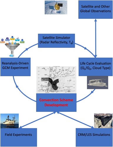
Convective parameterization is one of the most difficult problems in atmospheric sciences and requires long-term tedious work. Right now, most of the modelling centres are short of manpower working on convection scheme development, and the modern “bean counting” academic environment often prevent careful, deep work. It would be great if some fundings are secured to support a limited number of highly qualified researchers to focus on convection scheme development, which will reward global climate modelling in the long run.

Disclosure statement

No potential conflict of interest was reported by the author(s).

Additional information

Funding

Jialin Lin and Taotao Qian were supported by NSF [grant number AGS-1347132]. Part of this work was done by TQ when working in the Department of Geography, The Ohio State University. Guang Zhang was supported by NSF [grant number AGS-2054697]. Ping Zhu is supported by NOAA [grant numbers NA16NWS4680029 and NA18NWS4680057] and NSF [grant number AGS-1822238].

References

- Abercromby, R. (1888). First report of the thunderstorm committee. – On the photographs of lightning flashes. Quarterly Journal of the Royal Meteorological Society, 14, 226–234. https://doi.org/10.1002/qj.4970146707
- Agee, E. M. (1987). Mesoscale cellular convection over the oceans. Dynamics of Atmospheres and Oceans, 10, 317–341. https://doi.org/10.1016/0377-0265(87)90023-6
- Agee, E. M., Chen, T. S., & Dowell, K. E. (1973). A review of mesoscale cellular convection. Bulletin of the American Meteorological Society, 54(10), 1004–1012. https://doi.org/10.1175/1520-0477(1973)054<1004:AROMCC>2.0.CO;2
- Albrecht, B. A., Bretherton, C. S., Johnson, D., Schubert, W. H., & Frisch, A. S. (1995). The Atlantic stratocumulus transition experiment-ASTEX. Bulletin of the American Meteorological Society, 76(6), 889–904. https://doi.org/10.1175/1520-0477(1995)076<0889:TASTE>2.0.CO;2
- Albrecht, B. A., Penc, R. S., & Schubert, W. H. (1985). An observational study of cloud-topped mixed layers. Journal of the Atmospheric Society, 42(8), 800–822. https://doi.org/10.1175/1520-0469(1985)042<0800:AOSOCT>2.0.CO;2
- Albrecht, B. A., Randall, D. A., & Nicholls, S. (1988). Observations of marine stratocumulus during FIRE. Bulletin of the American Meteorological Society, 69(6), 618–626. https://doi.org/10.1175/1520-0477(1988)069<0618:OOMSCD>2.0.CO;2
- Albrecht, B., Ghate, V., Mohrmann, J., Wood, R., Zuidema, P., Bretherton, C., Schwartz, C., Eloranta, E., Glienke, S., Donaher, S., Sarkar, M., McGibbon, J., Nugent, A., Shaw, R. A., Fugal, J., Minnis, P., Paliknoda, R., Lussier, L., Jensen, J., … Schmidt, S. (2019). Cloud system evolution in the trades (CSET): Following the evolution of boundary layer cloud systems with the NSF-NCAR GV. Bulletin of the American Meteorological Society, 100(1), 93–121. https://doi.org/10.1175/BAMS-D-17-0180.1
- Alexander, G. D., & Cotton, W. R. (1998). The use of cloud-resolving simulations of mesoscale convective systems to build a mesoscale parameterization scheme. Journal of the Atmospheric Sciences, 55(12), 2137–2161. https://doi.org/10.1175/1520-0469(1998)055<2137:TUOCRS>2.0.CO;2
- Anderson, C. J., & Arritt, R. W. (1998). Mesoscale convective complexes and persistent elongated convective systems over the United States during 1992 and 1993. Monthly Weather Review, 126(3), 578–599. https://doi.org/10.1175/1520-0493(1998)126<0578:MCCAPE>2.0.CO;2
- Anthes, R. A. (1977). A cumulus parameterization scheme utilizing a one-dimensional cloud model. Monthly Weather Review, 105(3), 270–286. https://doi.org/10.1175/1520-0493(1977)105<0270:ACPSUA>2.0.CO;2
- Anthes, R. A., Hsie, E.-Y., & Kuo, Y. H. (1987). Description of the Penn State / NCAR Mesoscale Model Version 4(MM4). NCAR Tech. Rep. NCAR/TN-282+STR, 66 pp.
- Arakawa, A., Jung, J.-H., & Wu, C.-M. (2011). Toward unification of the multiscale modeling of the atmosphere. Atmos. Chem. Phys, 11(8), 3731–3742. https://doi.org/10.5194/acp-11-3731-2011
- Arakawa, A., & Schubert, W. H. (1974). Interaction of a cumulus cloud ensemble with the large-scale environment, Part I. Journal of the Atmospheric Sciences, 31(3), 674–701. https://doi.org/10.1175/1520-0469(1974)031<0674:IOACCE>2.0.CO;2
- Ashley, W. S., Mote, T. L., Dixon, P. G., Trotter, S. L., Powell, E. J., Durkee, J. D., & Grundstein, A. J. (2003). Distribution of mesoscale convective complex rainfall in the United States. Monthly Weather Review, 131(12), 3003–3017. https://doi.org/10.1175/1520-0493(2003)131<3003:DOMCCR>2.0.CO;2
- Augstein, E., Riehl, H., Ostapoff, F., & Wagner, V. (1973). Mass and energy transports in an undisturbed Atlantic trade-wind flow. Monthly Weather Review, 101(2), 101–111. https://doi.org/10.1175/1520-0493(1973)101<0101:MAETIA>2.3.CO;2
- Augustine, J. A., & Howard, K. W. (1988). Mesoscale convective complexes over the United States during 1985. Monthly Weather Review, 116(3), 685–701. https://doi.org/10.1175/1520-0493(1988)116<0685:MCCOTU>2.0.CO;2
- Austin, P. M., Rauber, R. M., Ochs IIIH. T., & Miller, L. J. (1996). Trade-wind clouds and Hawaiian rainbands. Monthly Weather Review, 124(10), 2126–2151. https://doi.org/10.1175/1520-0493(1996)124<2126:TWCAHR>2.0.CO;2
- Barnes, G. M., & Garstang, M. (1982). Subcloud layer energetics of precipitating convection. Monthly Weather Review, 110(2), 102–117. https://doi.org/10.1175/1520-0493(1982)110<0102:SLEOPC>2.0.CO;2
- Bechtold, P., Chaboureau, J. P., Beljaars, A., Betts, A. K., Kĥler, M., Miller, M., & Redelsperger, J. L. (2004). The simulation of the diurnal cycle of convective precipitation over land in a global model. Quarterly Journal of the Royal Meteorological Society, 130(604), 3119–3137. https://doi.org/10.1256/qj.03.103
- Bechtold, P., Kĥler, M., Jung, T., Leutbecher, M., Rodwell, M., Vitart, F., & Balsamo, G. (2008). Advances in predicting atmospheric variability with the ECMWF model from synoptic to decadal time-scales. Quarterly Journal of the Royal Meteorological Society, 134(634), 1337–1351. https://doi.org/10.1002/qj.289
- Bechtold, P., Krueger, S. K., Lewellen, W. S., van Meijgaard, E., Moeng, C.-H., Randall, D. A., van Ulden, A., & Wang, S. (1996). Modeling a stratocumulus-topped PBL: Intercompari- son among different one-dimensional codes and with large eddy simulation. Bulletin of the American Meteorological Society, 77(9), 2033–2042. https://doi.org/10.1175/1520-0477-77.9.2033
- Bechtold, P., Redelsperger, J.-L., Beau, I., Blackburn, M., Brinkop, S., Grandper, J.-Y., Grant, A., Gregory, D., Guichard, F., How, C., & Ioannidou, E. (2000). A GCSS model intercomparison for a tropical squall line observed during TOGA-COARE. II: Intercomparison of single-column models and a cloud-resolving model. Quarterly Journal of the Royal Meteorological Society, 126(564), 865–888. https://doi.org/10.1002/qj.49712656405
- Bechtold, P., Semane, N., Lopez, P., Chaboureau, J., Beljaars, A., & Bormann, N. (2014). Representing equilibrium and nonequilibrium convection in large-scale models. Journal of the Atmospheric Sciences, 71(2), 734–753. https://doi.org/10.1175/JAS-D-13-0163.1
- Becker, T., Bretherton, C. S., Hohenegger, C., & Stevens, B. (2018). Estimating bulk entrainment with unaggregated and aggregated convection. Geophysical. Research Letter, 45(1), 455–462. https://doi.org/10.1002/2017GL076640
- Becker, T., & Hohenegger, C. (2021). Entrainment and its dependency on environmental conditions and convective organization in convection-permitting simulations. Monthly Weather Review, 149(2), 537–550. https://doi.org/10.1175/MWR-D-20-0229.1
- Benard, H. (1900). Les tourbillons cellulaires dans une nappe liquide. Revue Generale des Sciences Pures et Appliquees, 11, 1261–1271 and 1309–1328.
- Bent, A. E. (1946). Radar detection of precipitation. Journal of the Atmospheric Sciences, 3(3), 78–84. https://doi.org/10.1175/1520-0469(1946)003<0078:RDOP>2.0.CO;2
- Bentsen, M., Bethke, I., Debernard, J. B., Iversen, T., KirkevÂg, A., Seland, ÿ., Drange, H., Roelandt, C., Seierstad, I. A., Hoose, C., & Kristjánsson, J. E. (2013). The Norwegian Earth System Model, NorESM1-M – Part 1: Description and basic evaluation of the physical climate. Geoscientific Model Development, 6, 687–720. https://doi.org/10.5194/gmd-6-687-2013
- Betts, A. K. (1973). Non-precipitating cumulus convection and its parameterization. Quarterly Journal of the Royal Meteorological Society, 99, 178–196. https://doi.org/10.1002/qj.49709941915
- Betts, A. K. (1975). Parametric interpretation of trade-wind cumulus budget studies. Journal of the Atmospheric Sciences, 32(10), 1934–1945. https://doi.org/10.1175/1520-0469(1975)032<1934:PIOTWC>2.0.CO;2
- Betts, A. K. (1986). A new convective adjustment scheme. Part I: Observational and theoretical basis. Quarterly Journal of the Royal Meteorological Society, 112(473), 677–691. https://doi.org/10.1002/qj.49711247307
- Betts, A. K., & Silva Dias, M. F. (1979). Unsaturated downdraft thermo- dynamics in cumulonimbus. Journal of the Atmospheric Sciences, 36(6), 1061–1071. https://doi.org/10.1175/1520-0469(1979)036<1061:UDTIC>2.0.CO;2
- Bjerknes, J. (1938). Saturated-adiabatic ascent of air through dry-adiabatically descending environment. Quarterly Journal of the Royal Meteorological Society, 64, 325–330.
- Bjerknes, J. (1969). Atmospheric teleconnections from the equatorial Pacific. Monthly Weather Review, 97(3), 163–172. https://doi.org/10.1175/1520-0493(1969)097<0163:ATFTEP>2.3.CO;2
- Black, M. L., Burpee, R. W., & Marks Jr, F. D. (1996). Vertical motion characteristics of tropical cyclones determined with airborne Doppler radial velocities. Journal of the Atmospheric Sciences, 53(13), 1887–1909. https://doi.org/10.1175/1520-0469(1996)053<1887:VMCOTC>2.0.CO;2
- Blamey, R. C., & Reason, C. J. C. (2013). The role of Mesoscale convective complexes in Southern Africa summer rainfall. Journal of Climate, 26(5), 1654–1668. https://doi.org/10.1175/JCLI-D-12-00239.1
- Blanchard, D. O. (1990). Mesoscale convective patterns of the Southern high plains. Bulletin of the American Meteorological Society, 71(7), 994–1005. https://doi.org/10.1175/1520-0477(1990)071<0994:MCPOTS>2.0.CO;2
- Bluestein, H. B., & Jain, M. H. (1985). Formation of mesoscale lines of precipitation: Severe squall lines in Oklahoma during the spring. Journal of the Atmospheric Sciences, 42(16), 1711–1732. https://doi.org/10.1175/1520-0469(1985)042<1711:FOMLOP>2.0.CO;2
- Bluestein, H. B., & Parks, C. R. (1983). Synoptic and photographic climatology of low-precipitation severe thunderstorms in the southern plains. Monthly Weather Review, 111(10), 2034–2046. https://doi.org/10.1175/1520-0493(1983)111<2034:ASAPCO>2.0.CO;2
- Bodas-Salcedo, A., Webb, M. J., Bony, S., Chepfer, H., Dufresne, J.-L., Klein, S. A., Zhang, Y., Marchand, R., Haynes, J. M., Pincus, R., & John, V. O. (2011). COSP satellite simulation software for model assessment. Bulletin of the American Meteorological Society, 92(8), 1023–1043. https://doi.org/10.1175/2011BAMS2856.1
- Boer, G. J., Smith, D. M., Cassou, C., Doblas-Reyes, F., Danabasoglu, G., Kirtman, B., Kushnir, Y., Kimoto, M., Meehl, G. A., Msadek, R., Mueller, W. A., Taylor, K. E., Zwiers, F., Rixen, M., Ruprich-Robert, Y., & Eade, R. (2016). The decadal climate prediction project (DCPP) contribution to CMIP6. Geoscientific Model Development, 9(10), 3751–3777. https://doi.org/10.5194/gmd-9-3751-2016
- Bogenschutz, P. A., Gettelman, A., Morrison, H., Larson, V. E., Craig, C., & Schanen, D. P. (2013). Higher-order turbulence closure and its impact on climate simulations in the Community Atmosphere Model. Journal of Climate, 26(23), 9655–9676. https://doi.org/10.1175/JCLI-D-13-00075.1
- Bony, S., & Dufresne, J. L. (2005). Marine boundary layer clouds at the heart of tropical cloud feedback uncertainties in climate models. Geophysical Research Letter, 32(20), L20806. https://doi.org/10.1029/2005GL023851
- Bony, S., Stevens, B., Frierson, D. M. W., Jakob, C., Kageyama, M., Pincus, R., Shepherd, T. G., Sherwood, S. C., Pier Siebesma, A., Sobel, A. H., Watanabe, M., & Webb, M. J. (2015). Clouds, circulation and climate sensitivity. Nature Geoscience, 8, 261–268. https://doi.org/10.1038/ngeo2398
- Bougeault, P. (1981). Modeling the trade-wind cumulus boundary layer. Part II: Ahigher-order one-dimensional model. Journal of the Atmospheric Sciences, 38(11), 2429–2439. https://doi.org/10.1175/1520-0469(1981)038<2429:MTTWCB>2.0.CO;2
- Bougeault, P. (1985). A simple parameterization of the large-scale effects of cumulus convection. Monthly Weather Review, 113(12), 2108–2121. https://doi.org/10.1175/1520-0493(1985)113<2108:ASPOTL>2.0.CO;2
- Bretherton, C., et. al. (2004). The EPIC 2001 stratocumulus study. Bulletin of American Meteorological Society, 85, 967–977. doi:10.1175/BAMS-85-7-967
- Bretherton, C. S., Blossey, P. N., & Jones, C. (2013). Mechanisms of marine low cloud sensitivity to idealized climate perturbations: A single-LES exploration extending the CGILS cases. Journal of Advanced Modeling of Earth System, 5, 316–337. doi:10.1002/jame.20019
- Bretherton, C. S., Blossey, P. N., & Khairoutdinov, M. (2005). An energy-balance analysis of deep convective self- aggregation above uniform SST. Journal of the Atmospheric Sciences, 62(12), 4273–4292. https://doi.org/10.1175/JAS3614.1
- Bretherton, C. S., George, R., Wood, R., Allen, G., Leon, D., & Albrecht, B. (2010). Southeast Pacific stratocumulus clouds, precipitation and boundary layer structure sampled along 20S during VOCALS-REx. Atmospheric Chemistry and Physics, 10, 10639–10654. doi:10.5194/acp-10-10639-2010
- Bretherton, C. S., McCaa, J. R., & Grenier, H. (2004a). A new parameterization for shallow cumulus convection and its application to marine subtropical cloud-topped boundary layers. Part I: Description and 1D results. Monthly Weather Review, 132(4), 864–882. https://doi.org/10.1175/1520-0493(2004)132<0864:ANPFSC>2.0.CO;2
- Bretherton, C. S., & Park, S. (2009). A new moist turbulence parameterization in the Community Atmospheric Model. Journal of Climate, 22(12), 3422–3448. https://doi.org/10.1175/2008JCLI2556.1
- Bretherton, C. S., Uttal, T., Fairall, C. W., Yuter, S. E., Weller, R. A., Baumgardner, D., Comstock, K., & Wood, R. (2004b). The EPIC 2001 stratocumulus study. Bulletin of the American Meteorological Society, 85(7), 967–977. https://doi.org/10.1175/BAMS-85-7-967
- Brient, F., & Bony, S. (2013). Interpretation of the positive low-cloud feedback predicted by a climate model under global warming. Climate Dynamics, 40, 2415–2431. doi:10.1007/s00382-011-1279-7
- Brocks, K. (1972). Die Atlantische Expedition 1969 (GARP) mit dem Atlantischen Passat Experiment (APEX). Meteor-Forschung- sergebnisse, Ser. A, No. 9.
- Brown, R. G., & Bretherton, C. S. (1997). A test of the strict quasi- equilibrium theory on long time and space scales. Journal of the Atmospheric Sciences, 54(5), 624–638. https://doi.org/10.1175/1520-0469(1997)054<0624:ATOTSQ>2.0.CO;2
- Brown, R. G., & Zhang, C. (1997). Variability of midtropospheric moisture and its effect on cloud-top height distribution dur- ing TOGA COARE. Journal of the Atmospheric Sciences, 54(23), 2760–2774. https://doi.org/10.1175/1520-0469(1997)054<2760:VOMMAI>2.0.CO;2
- Browning, K. A. (1964). Airflow and precipitation trajectories within severe local storms which travel to the right of the winds. Journal of the Atmospheric Sciences, 21(6), 634–639. https://doi.org/10.1175/1520-0469(1964)021<0634:AAPTWS>2.0.CO;2
- Brummer, B. (1978). Mass and energy budgets of a 1-km high atmospheric box over the GATE C-scale triangle during undis- turbed and disturbed weather conditions. Journal of the Atmospheric Sciences, 35(6), 997–1011. https://doi.org/10.1175/1520-0469(1978)035<0997:MAEBOA>2.0.CO;2
- Bryan, G. H., & Parker, M. D. (2010). Observations of a squall line and its near environment using high- frequency rawinsonde launches during VORTEX2. Monthly Weather Review, 138(11), 4076–4097. https://doi.org/10.1175/2010MWR3359.1
- Byers, H. R., & Battan, L. J. (1949). Some effects of vertical wind shear on thunderstorm structure. Bulletin of the American Meteorological Society, 30(5), 168–175. https://doi.org/10.1175/1520-0477-30.5.168
- Byers, H. R., & Braham, R. R. (1948). Thunderstorm circulation and structure. Journal of Meteorology, 5(3), 71–86. https://doi.org/10.1175/1520-0469(1948)005%3C0071:TSAC%3E2.0.CO;2
- Byers, H. R., Holzman, B. G., & Maynard, R. H. (1946). A project on thunderstorm microstructure. Bulletin of the American Meteorological Society, 27(4), 143–146. https://doi.org/10.1175/1520-0477-27.4.143
- Byers, H. R., & Hull, E. (1949). Inflow patterns of thunderstorms as shown by winds aloft. Bulletin of the American Meteorological Society, 30(3), 90–96. https://doi.org/10.1175/1520-0477-30.3.90
- Byers, H. R., & Rodebush, H. R. (1948). Causes of thunderstorms of the Florida peninsula. Journal of Meteorology, 5(6), 275–280. https://doi.org/10.1175/1520-0469(1948)005%3C0275:COTOTF%3E2.0.CO;2
- Caldwell, P., & Bretherton, C. S. (2009). Response of a subtropical stratocumulus-capped mixed layer to climate and aerosol changes. Journal of Climate, 22, 20–38. doi:10.1175/2008JCLI1967.1
- Cao, G., & Zhang, G. J. (2017). Role of vertical structure of convective heating in MJO simulation in NCAR CAM5.3. Journal of Climate, 30(18), 7423–7439. https://doi.org/10.1175/JCLI-D-16-0913.1
- Chikira, M., & Sugiyama, M. (2010). A cumulus parameterization with state-dependent entrainment rate. Part I: Description and sensitivity to temperature and humidity profiles. Journal of the Atmospheric Sciences, 67(7), 2171–2193. https://doi.org/10.1175/2010JAS3316.1
- Christensen, H. M., Dawson, A., & Holloway, C. E. (2018). Forcing single-column models using high-resolution model simulations. Journal of Advances Modeling Earth Systems, 10(8), 1833–1857. https://doi.org/10.1029/2017MS001189
- Cotton, W. R., Lin, M. S., McAnelly, R. L., & Tremback, C. J. (1989). A composite model of mesoscale convective complexes. Monthly Weather Review, 117(4), 765–783. https://doi.org/10.1175/1520-0493(1989)117<0765:ACMOMC>2.0.CO;2
- Covey, C., Gleckler, P. J., Doutriaux, C., Williams, D. N., Dai, A., Fasullo, J., Trenberth, K., & Berg, A. (2016). Metrics for the diurnal cycle of precipitation: Toward routine benchmarks for climate models. Journal of Climate, 29(12), 4461–4471. https://doi.org/10.1175/JCLI-D-15-0664.1
- Curry, J. A., Hobbs, P. V., King, M. D., Randall, D. A., Minnis, P., Isaac, G. A., Pinto, J. O., Uttal, T., Bucholtz, A., Cripe, D. G., Gerber, H., Fairall, C. W., Garrett, T. J., Hudson, J., Intrieri, J. M., Jakob, C., Jensen, T., Lawson, P., Marcotte, D., … Wylie, D. (2000). FIRE Arctic clouds experiment. Bulletin of the American Meteorological Society, 81(1), 5–29. https://doi.org/10.1175/1520-0477(2000)081<0005:FACE>2.3.CO;2
- Dai, A. (2006). Precipitation characteristics in eighteen coupled climate models. Journal of Climate, 19(18), 4605–4630. https://doi.org/10.1175/JCLI3884.1
- Dal Gesso, S., van der Dussen, J. J., Siebesma, A. P., de Roode, S. R., Boutle, I. A., Kamae, Y., Roehrig, R., & Vial, J. (2015). A single-column model intercomparison on the stratocumulus representation in present-day and future climate. Journal of Advances in Modeling Earth Systems, 7(2), 617–647. https://doi.org/10.1002/2014MS000377
- D’Andrea, F., Gentine, P., Betts, A. K., & Lintner, B. R. (2014). Triggering deep convection with a probabilistic plume model. Journal of the Atmospheric Sciences, 71(11), 3881–3901. https://doi.org/10.1175/JAS-D-13-0340.1
- Das, P., & Subba Rao, M. C. (1972). The unsaturated downdraft. Indian Journal of Meteorological Geophysics, 23, 135–144.
- Davies, L., Jakob, C., Cheung, K., Del Genio, A., Hill, A., Hume, T., Keane, R. J., Komori, T., Larson, V. E., Lin, Y., Liu, X., Nielsen, B. J., Petch, J., Plant, R. S., Singh, M. S., Shi, X., Song, X., Wang, W., Whitall, M. A., … Zhang, G. (2013). A single-column model ensemble approach applied to the TWP-ICE experiment. Journal of Geophysical Research, 118(12), 1–20. https://doi.org/10.1002/jgrd.50450
- Deardorff, J. W. (1980). Cloud top entrainment instability. Journal of the Atmospheric Sciences, 37(1), 131–147. https://doi.org/10.1175/1520-0469(1980)037<0131:CTEI>2.0.CO;2
- Del Genio, A. D., & Wu, J. (2010). The role of entrainment in the diurnal cycle of continental convection. Journal of Climate, 23(10), 2722–2738. https://doi.org/10.1175/2009JCLI3340.1
- Del Genio, A. D., & Yao, M. S. (1993). Efficient cumulus pa- rameterization for long-term climate studies: The GISS scheme. The Representation of Cumulus Convection in Numerical Models, Meteorological Monographs, 46, 181–184. American Meteorological Society.
- Deng, A., Seaman, N. L., & Kain, J. S. (2003a). A shallow-convection parameterization for mesoscale models Part I: Sub-model description and preliminary applications. Journal of the Atmospheric Sciences, 60(1), 34–56. https://doi.org/10.1175/1520-0469(2003)060<0034:ASCPFM>2.0.CO;2
- Deng, A., Seaman, N. L., & Kain, J. S. (2003b). A shallow-convection parameterization for mesoscale models Part II. Verification and sensitivity studies. Journal of the Atmospheric Sciences, 60(1), 57–78. https://doi.org/10.1175/1520-0469(2003)060<0057:ASCPFM>2.0.CO;2
- Derbyshire, S. H., Beau, I., Bechtold, P., Grandpeix, J. Y., Piriou, J. M., Redelsperger, J. L., & Soares, P. M. M. (2004). Sensitivity of moist convection to environmental humidity. Quarterly Journal of the Royal Meteorological Society, 130(604), 3055–3079. https://doi.org/10.1256/qj.03.130
- de Rooy, W., Bechtold, P., Frohlich, K., Hohenegger, C., Jonker, H., Mironov, S., Teixeira, J., & Yano, J. I. (2013). Entrainment and detrainment in cumulus convection: An overview. Quarterly Journal of the Royal Meteorological Society, 139, 1–19. https://doi.org/10.1002/qj.1959
- de Szoeke, S. P., Skyllingstad, E. D., Zuidema, P., & Chandra, A. S. (2017). Cold pools and their influence on the tropical marine boundary layer. Journal of the Atmospheric Sciences, 74(4), 1149–1168. https://doi.org/10.1175/JAS-D-16-0264.1
- Donner, L. J. (1993). A cumulus parameterization including mass fluxes, vertical momentum dynamics, and mesoscale effects. Journal of the Atmospheric Sciences, 50(6), 889–906. https://doi.org/10.1175/1520-0469(1993)050<0889:ACPIMF>2.0.CO;2
- Donner, L. J., O’Brien, T. A., Rieger, D., Vogel, B., & Cooke, W. F. (2016). Are atmospheric updrafts a key to unlocking climate forcing and sensitivity? Atmospheric Chemistry Physics, 16(20), 12,983–12,992. https://doi.org/10.5194/acp-16-12983-2016
- Donner, L. J., & Phillips, V. T. (2003). Boundary layer control on convective available potential energy: Implications for cumulus parameterization. Journal of Geophysical Research, 108(D22), 4701. https://doi.org/10.1029/2003JD003773
- Donner, L. J., Phillips, V. T., Hemler, R. S., & Fan, S. (2001). A cumulus parameterization including mass fluxes, convective vertical velocities, and mesoscale effects: Thermodynamic and hydrological aspects in a general circulation model. Journal of Climate, 14(16), 3444–3463. https://doi.org/10.1175/1520-0442(2001)014<3444:ACPIMF>2.0.CO;2
- Donner, L. J., Wyman, B. L., Hemler, R. S., Horowitz, L. W., Ming, Y., Zhao, M., Golaz, J.-C., Ginoux, P., Lin, S.-J., Schwarzkopf, M. D., Austin, J., Alaka, G., Cooke, W. F., Delworth, T. L., Freidenreich, S. M., Gordon, C. T., Griffies, S. M., Held, I. M., Hurlin, W. J., … Zeng, F. (2011). The dynamical core, physical parameterizations, and basic simulation characteristics of the atmospheric component AM3 of the GFDL global coupled model CM3. Journal of Climate, 24(13), 3484–3519. https://doi.org/10.1175/2011JCLI3955.1
- Dos Santos, A. F., de Campos Velho, H. F., Luz, E. F. P., Saulo, F. R., Grell, G., & Gan, M. A. (2013). Firefly optimization to determine the precipitation field on South America. Inverse Problems in Science and Engineering, 21(3), 451–466. https://doi.org/10.1080/17415977.2012.712531
- Durkee, J. D., Mote, T. L., & Sheppard, J. M. (2009). The contribution of meso-scale convective complexes to rainfall across subtropical South America. Journal of Climate, 22(17), 4590–4605. https://doi.org/10.1175/2009JCLI2858.1
- Emanuel, K. (1995). The behavior of a simple hurricane model using a convective scheme based on subcloud layer entropy equilibrium. Journal of the Atmospheric Sciences, 52(22), 3960–3968. https://doi.org/10.1175/1520-0469(1995)052<3960:TBOASH>2.0.CO;2
- Emanuel, K. (2007). Quasi-equilibrium dynamics of the tropical atmosphere. In T. Schneider & A. Sobel (Eds.), The Global Circulation of the Atmosphere (pp. 186–218). Princeton University Press.
- Emanuel, K. A. (1981). A similarity theory for unsaturated downdrafts within clouds. Journal of the Atmospheric Sciences, 38(8), 1541–1557. https://doi.org/10.1175/1520-0469(1981)038<1541:ASTFUD>2.0.CO;2
- Emanuel, K. A. (1991). A scheme for representing cumulus convection in large-scale models. Journal of the Atmospheric Sciences, 48(21), 2313–2335. https://doi.org/10.1175/1520-0469(1991)048<2313:ASFRCC>2.0.CO;2
- Emanuel, K., Neelin, J. D., & Bretherton, C. S. (1994). On large-scale circulation in convective atmospheres. Quarterly Journal of the Royal Meteorological Society, 120, 1111–1143. https://doi.org/10.1002/qj.49712051902
- Engerer, N. A., Stensrud, D. J., & Coniglio, M. C. (2008). Surface characteristics of observed cold pools. Monthly Weather Review, 136(12), 4839–4849. https://doi.org/10.1175/2008MWR2528.1
- Esbensen, S. (1975). An analysis of subcloud-layer heat and moisture budgets in the western Atlantic trades. Journal of the Atmospheric Sciences, 32(10), 1921–1933. https://doi.org/10.1175/1520-0469(1975)032<1921:AAOSLH>2.0.CO;2
- Esbensen, S. (1978). Bulk thermodynamic effects and properties of small tropical cumuli. Journal of the Atmospheric Sciences, 35(5), 826–837. https://doi.org/10.1175/1520-0469(1978)035<0826:BTEAPO>2.0.CO;2
- Eyring, V., Bock, L., Lauer, A., Righi, M., Schlund, M., Andela, B., Arnone, E., Bellprat, O., Brötz, B., Caron, L.-P., Carvalhais, N., Cionni, I., Cortesi, N., Crezee, B., Davin, E. L., Davini, P., Debeire, K., de Mora, L., Deser, C., … Zimmermann, K. (2020). Earth System Model evaluation Tool (ESMValTool) v2.0 – an extended set of large-scale diagnostics for quasi-operational and comprehensive evaluation of Earth system models in CMIP. Geoscientific Model Development, 13(7), 3383–3438. https://doi.org/10.5194/gmd-13-3383-2020
- Eyring, V., Cox, P. M., Flato, G. M., Gleckler, P. J., Abramowitz, G., Caldwell, P., Collins, W. D., Gier, B. K., Hall, A. D., & Hoffman, F. M. J. N. C. C. (2019). Taking climate model evaluation to the next level. Nature Climate Change, 9, 102–110. https://doi.org/10.1038/s41558-018-0355-y
- Eyring, V., Gleckler, P. J., Heinze, C., Stouffer, R. J., Taylor, K. E., Balaji, V., Guilyardi, E., Joussaume, S., Kindermann, S., Lawrence, B. N., Meehl, G. A., Righi, M., & Williams., D. N. (2016). Towards improved and more routine Earth system model evaluation in CMIP. Earth System Dynamics, 7(4), 813–830. https://doi.org/10.5194/esd-7-813-2016
- Feynman, R. P., Leighton, R. B., & Sands, M. (1965). The Feynman lectures on physics vol. 2. Addison-Wesley. 538pp.
- Ficker, H. V. (1936). Bemerkungen uber den Warmeumstaz innerhalb der Passatzirkulation. Vcrlag Akademische WissenSchaften.
- Fortune, M. A., Cotton, W. R., & McAnelly, R. L. (1992). Frontal-wave-like evolution in some mesoscale convective complexes. Monthly Weather Review, 120(7), 1279–1300. https://doi.org/10.1175/1520-0493(1992)120<1279:FWLEIS>2.0.CO;2
- Fovell, R. G., & Ogura, Y. (1988). Numerical simulation of a midlatitude squall line in two dimensions. Journal of the Atmospheric Sciences, 45(24), 3846–3879. https://doi.org/10.1175/1520-0469(1988)045<3846:NSOAMS>2.0.CO;2
- Fowler, L. D., Skamarock, W. C., Grell, G. A., Freitas, S. R., & Duda, M. G. (2016). Analyzing the Grell–Freitas convection scheme from hydrostatic to nonhydrostatic scales within a global model. Monthly Weather Review, 144(6), 2285–2306. https://doi.org/10.1175/MWR-D-15-0311.1
- Frank, W. M., & Cohen, C. (1987). Simulation of tropical convective systems. Part I: A cumulus parameterization. Journal of the Atmospheric Sciences, 44(24), 3787–3799. https://doi.org/10.1175/1520-0469(1987)044<3787:SOTCSP>2.0.CO;2
- Frank, W. M., & McBride, J. L. (1989). The vertical distribution of heating in AMEX and GATE cloud clusters. Journal of the Atmospheric Sciences, 46(22), 3464–3478. https://doi.org/10.1175/1520-0469(1989)046<3464:TVDOHI>2.0.CO;2
- Frank, W. M., Wang, H., & McBride, J. L. (1996). Rawinsonde budget analyses during the TOGA COARE IOP. Journal of the Atmospheric Sciences, 53(13), 1761–1780. https://doi.org/10.1175/1520-0469(1996)053<1761:RBADTT>2.0.CO;2
- Franklin, C. N., Protat, A., Leroy, D., & Fontaine, E. (2016). Controls on phase composition and ice water content in a convection- permitting model simulation of a tropical mesoscale convective system. Atmospheric Chemistry Physics, 16(14), 8767–8789. https://doi.org/10.5194/acp-16-8767-2016
- Freitas, S. R., Grell, G. A., & Li, H. (2021). The GF convection parameterization: Recent developments, extensions, and applications. Geoscientific Model Development, 14(9), 5393–5411. https://doi.org/10.5194/gmd-14-5393-2021
- Freitas, S. R., Grell, G. A., Molod, A., Thompson, M. A., Putman, W. M., Silva, S. e., & Souza, C. M., & P, E. (2018). Assessing the Grell-Freitas convection parameterization in the NASA GEOS modeling system. Journal of Advances in Modeling Earth Systems, 10(6), 1266–1289. https://doi.org/10.0.1029/2017MS001251
- Freitas, S. R., Panetta, J., Longo, K. M., Rodrigues, L. F., Moreira, D. S., Rosário, N. E., Dias, P. L. S., Dias, M. A. F. S., Souza, E. P., Freitas, E. D., Longo, M., Frassoni, A., Fazenda, A. L., M, C., Silva, S. e., Pavani, C. A. B., Eiras, D., França, D. A., Massaru, D., … Martins, L. D. (2017). The Brazilian developments on the regional atmospheric modeling system (BRAMS 5.2): An integrated environmental model tuned for tropical areas. Geoscientific Model Development, 10(1), 189–222. [10.5194/gmd-10-189-2017].
- Freitas, S. R., Putman, W. M., Arnold, N. P., Adams, D. K., & Grell, G. A. (2020). Cascading toward a kilometer-scale GCM: Impacts of a scale-aware convection parameterization in the Goddard earth observing system GCM. Geophysical Research Letter, 47, e2020GL087682. https://doi.org/10.1029/2020GL087682
- Fridlind, A. M., Li, X., Wu, D., van Lier-Walqui, M., Ackerman, A. S., Tao, W.-K., McFarquhar, G. M., Wu, W., Dong, X., Wang, J., Ryzhkov, A., Zhang, P., Poellot, M. R., Neumann, A., & Tomlinson, J. M. (2017). Derivation of aerosol profiles for MC3E convection studies and use in simulations of the 20 May squall line case. Atmospheric Chemistry Physics, 17(9), 5947–5972. https://doi.org/10.5194/acp-17-5947-2017
- Fritsch, J. M., & Chappell, C. F. (1980). Numerical prediction of convectively driven mesoscale pressure systems. Part I: Convective parameterization. Journal of the Atmospheric Sciences, 37(8), 1722–1733. https://doi.org/10.1175/1520-0469(1980)037<1722:NPOCDM>2.0.CO;2
- Fujita, T. (1958). Mesoanalysis of the Illinois tornadoes of 9 April 1953. Journal of Meteorology, 15(3), 288–296. https://doi.org/10.1175/1520-0469(1958)015%3C0288:MOTITO%3E2.0.CO;2
- Fujiwhara, S. (1939). The law of disturbance. Proceedings of the Imperial Academy, 15(9), 292–297. https://doi.org/10.2183/pjab1912.15.292
- Gallus, W. A., & Johnson, R. H. (1991). Heat and moisture budgets of an intense midlatitude squall line. Journal of the Atmospheric Sciences, 48(1), 122–146. https://doi.org/10.1175/1520-0469(1991)048<0122:HAMBOA>2.0.CO;2
- Gallus, W. A., & Johnson, R. H. (1992). The momentum budget of an intense midlatitude squall line. Journal of the Atmospheric Sciences, 49(5), 422–450. https://doi.org/10.1175/1520-0469(1992)049<0422:TMBOAI>2.0.CO;2
- Gamache, J. F., & Houze, R. A. (1983). Water budget of a mesoscale convective system in the tropics. Journal of the Atmospheric Sciences, 40(7), 1835–1850. https://doi.org/10.1175/1520-0469(1983)040<1835:WBOAMC>2.0.CO;2
- Gates, W. L., Boyle, J. S., Covey, C., Dease, C. G., Doutriaux, C. M., Drach, R. S., Fiorino, M., Gleckler, P. J., Hnilo, J. J., Marlais, S. M., Phillips, T. J., Potter, G. L., Santer, B. D., Sperber, K. R., Taylor, K. E., & Williams, D. N. (1999). An overview of the results of the Atmospheric Model Intercomparison Project (AMIP-I). Bulletin of the American Meteorological Society, 80(1), 29–55. https://doi.org/10.1175/1520-0477(1999)080<0029:AOOTRO>2.0.CO;2
- Gentine, P., Pritchard, M., Rasp, S., Reinaudi, G., & Yacalis, G. (2018). Could machine learning break the convection parameterization deadlock? Geophysical Research Letter, 45(11), 5742–5751. https://doi.org/10.1029/2018GL078202
- Gerard, L. (2015). Bulk mass-flux perturbation formulation for a unified approach of deep convection at high resolution. Monthly Weather Review, 143(10), 4038–4063. https://doi.org/10.1175/MWR-D-15-0030.1
- Ghan, S., Randall, D., Xu, K.-M., Cederwall, R., Cripe, D., Hack, J., Iacobellis, S., Klein, S., Krueger, S., Lohmann, U., Pedretti, J., Robock, A., Rotstayn, L., Somerville, R., Stenchikov, G., Sud, Y., Walker, G., Xie, S., Yio, J., & Zhang, M. (2000). A comparison of single column model simulations of summertime midlatitude continental convection. Journal of Geophysical Research, 105(D2), 2091–2124. https://doi.org/10.1029/1999JD900971
- Ghate, V. P., Albrecht, B. A., & Kollias, P. (2010). Vertical velocity struc- ture of nonprecipitating continental boundary layer stratocumulus clouds. Journal of Geophysical Research, 115(D13), D13204. https://doi.org/10.1029/2009JD013091
- Ghate, V. P., Miller, M. A., & DiPretore, L. (2011). Vertical velocity structure of marine boundary layer trade wind cumulus clouds. Journal of Geophysical Research, 116(D16), 2156–2202. https://doi.org/10.1029/2010JD015344
- Giangrande, S. E., Collis, S., Straka, J., Protat, A., Williams, C., & Krueger, S. (2013). A summary of convective-core vertical velocity properties using ARM UHF wind profilers in Oklahoma. Journal of Applied Meteorological Climatology, 52(10), 2278–2295. https://doi.org/10.5194/acp-17-14519-2017
- Giangrande, S. E., Toto, T., Jensen, M. P., Bartholomew, M. J., Feng, Z., Protat, A., Williams, C. R., Schumacher, C., & Machado, L. (2016). Convective cloud vertical velocity and mass-flux characteristics from radar wind profiler observations during GoAmazon2014/5. Journal of Geophysics Research, 121(21), 12,891–12,913. https://doi.org/10.1002/2016JD025303
- Giblett, M. A. (1923). Upper air conditions after a line-squall. Nature, 112, 863–864.
- Gidel, L. T. (1983). Cumulus cloud transport of transient tracers. Journal of Geophysical Research - Oceans, 88(C11), 6587–6599. https://doi.org/10.1029/JC088iC11p06587
- Giorgi, F., Coppola, E., Solmon, F., Mariotti, L., Sylla, M. B., Bi, X., Elguindi, N., Diro, G. T., Nair, V., Giuliani, G., Turuncoglu, U. U., Cozzini, S., Güttler, I., O’Brien, T. A., Tawfik, A. B., Shalaby, A., Zakey, A. S., Steiner, A. L., Stordal, F., & Sloan, L. C. (2012). RegCM4: Model description and preliminary tests over multiple CORDEX domains. Climate Research, 52, 7–29. https://doi.org/10.3354/cr01018
- Golaz, J. C., Larson, V. E., & Cotton, W. R. (2002). A pdf-based model for boundary layer clouds: Part I. Method and model description. Journal of the Atmospheric Sciences, 59(24), 3540–3551. https://doi.org/10.1175/1520-0469(2002)059<3540:APBMFB>2.0.CO;2
- Goswami, B., Khouider, B., Phani, R., Mukhopadhyay, P., & Majda, A. (2017). Improving synoptic and intraseasonal variability in cfsv2 via stochastic representation of organized convection. Geophysical Research Letter, 44(2), 1104–1113. https://doi.org/10.1002/2016GL071542
- Grabowski, W. W., Bechtold, P., Cheng, A., Forbes, R., Halliwell, C., Khairoutdinov, M., Lang, S., Nasuno, T., Petch, J., Tao, W.-K., Wong, R., Wu, X., & Xu, K.-M. (2006). Daytime convective development over land: A model intercomparison based on LBA observations. Quarterly Journal of the Royal Meteorological Society, 132, 317–344. https://doi.org/10.1256/qj.04.147
- Grandpeix, J., & Lafore, J. (2010). A density current parameterization coupled with Emanuel’s convection scheme. Part I: The models. Journal of the Atmospheric Sciences, 67(4), 881–897. https://doi.org/10.1175/2009JAS3044.1
- Grandpeix, J., Lafore, J., & Cheruy, F. (2010). A density current parameterization coupled with Emanuel’s convection scheme. Part II: 1D simulations. Journal of the Atmospheric Sciences, 67(4), 898–922. https://doi.org/10.1175/2009JAS3045.1
- Grandpeix, J. Y., Phillips, V., & Tailleux, R. (2004). Improved mixing representation in Emanuel's convection scheme. Quarterly Journal of the Royal Meteorological Society, 130(604), 3207–3222. https://doi.org/10.1256/qj.03.144
- Gregory, D., Morcrette, J. J., Jakob, C., Beljaars, A., & Stockdale, T. (2000). Revision of convection, radiation and cloud schemes in the ECMWF integrated forecasting system. Quarterly Journal of the Royal Meteorological Society, 134(586), 1337–1351. https://doi.org/10.1002/qj.49712656607
- Gregory, D., & Rowntree, P. R. (1990). A mass flux convection scheme with representation of cloud ensemble characteristics and stability-dependent closure. Monthly Weather Review, 118(7), 1483–1506. https://doi.org/10.1175/1520-0493(1990)118<1483:AMFCSW>2.0.CO;2
- Grell, G. A. (1988). Semi-prognostic tests of cumulus parameterization schemes in the middle latitudes [PhD dissertation]. University of Miami, Coral Gables, Florida, 225 pp.
- Grell, G. A. (1993). Prognostic evaluation of assumptions used by cumulus parameterizations. Monthly Weather Review, 121(3), 764–787. https://doi.org/10.1175/1520-0493(1993)121<0764:PEOAUB>2.0.CO;2
- Grell, G. A., & Devenyi, D. (2002). A generalized approach to parameterizing convection combining ensemble and data assimilation techniques. Geophysical Research Letter, 29, 38-1–38-4. https://doi.org/10.1029/2002GL015311
- Grell, G. A., & Freitas, S. R. (2014). A scale and aerosol aware stochastic convective parameterization for use in weather and air quality modelling. Atmospheric Chemistry Physics, 14, 5233–5250. https://doi.org/10.1007/978-94-007-5577-2_60
- Grell, G. A., Kuo, Y. H., & Pasch, R. (1991). Semi-prognostic tests of cumulus parameterization schemes in the middle latitudes. Monthly Weather Review, 119(1), 5–31. https://doi.org/10.1175/1520-0493(1991)119<0005:STOCPS>2.0.CO;2
- Grenier, H., & Bretherton, C. S. (2001). A moist PBL parame- terization for large-scale models and its application to sub- tropical cloud-topped marine boundary layers. Monthly Weather Review, 129(3), 357–377. https://doi.org/10.1175/1520-0493(2001)129,0357:AMPPFL.2.0.CO;2
- Grim, J. A., Rauber, R. M., McFarquhar, G. M., & Jewett, B. F. (2009). Development and forcing of the rear inflow jet in a rapidly developing and decaying squall line during BAMEX. Monthly Weather Review, 137(4), 1206–1229. https://doi.org/10.1175/2008MWR2503.1
- Gu, J. F., Plant, R. S., Holloway, C. E., Jones, T. R., Stirling, A., Clark, P. A., … Webb, T. L. (2020). Evaluation of the bulk mass flux formulation using large-eddy simulations. Journal of the Atmospheric Sciences, 77(6), 2115–2137. https://doi.org/10.1175/JAS-D-19-0224.1
- Guichard, F., Petch, J. C., Redelsperger, J.-L., Bechtold, P., Chaboureau, J.-P., Cheinet, S., Grabowski, W., Grenier, H., Jones, C. G., Köhler, M., Piriou, J.-M., Tailleux, R., & Tomasini, M. (2004). Modelling the diurnal cycle of deep precipitating convection over land with cloud-resolving models and single-column models. Quarterly Journal of the Royal Meteorological Society, 130(604C), 3139–3172. https://doi.org/10.1256/qj.03.145
- Guo, H., Golaz, J. C., Donner, L. J., Wyman, B., Zhao, M., & Ginoux, P. (2015). CLUBB as a unified cloud parameterization: Opportunities and challenges. Geophysical Research Letter, 42, 4540–4547. https://doi.org/10.1002/2015GL063672
- Hadley, G. (1735). Concerning the cause of the general trade-winds. Philosophical Transactions, The Royal Society, 39(437), 58–62. https://doi.org/10.1098/rstl.1735.0014
- Hagos, S., Feng, Z., Plant, R. S., Houze, J. R. A., & Xiao, H. (2018). A stochastic framework for modeling the population dynamics of convective clouds. Journal of Advances in Modeling Earth Systems, 10(2), 448–465. https://doi.org/10.1002/2017MS001214
- Hagos, S., Leung, L. R., & Dudhia, J. (2010). Thermodynamics of Madden Julian Oscillation in a regional model with constrained moistening. Journal of the Atmospheric Sciences, 68(9), 1974–1989. https://doi.org/10.1175/2011JAS3592.1
- Hamilton, R. A., & Archbold, J. W. (1945). Meteorology of Nigeria and adjacent territory. Quarterly Journal of the Royal Meteorological Society, 71(309–310), 231–262. https://doi.org/10.1002/qj.49707130905
- Han, B., Fan, J., Varble, A., Morrison, H., Williams, C. R., Chen, B., Dong, X., Giangrande, S. E., Khain, A., Mansell, E., Milbrandt, J. A., Shpund, J., & Thompson, G. (2019). Cloud-resolving model intercomparison of an MC3E squall line case: Part II. Stratiform precipitation properties. Journal of Geophysical Research, 124(2), 1090–1117. https://doi.org/10.1029/2018JD029596
- Han, J., & Pan, H. L. (2011). Revision of convection and vertical diffusion schemes in the NCEP global forecast system. Weather and Forecasting, 26(4), 520–533. https://doi.org/10.1175/WAF-D-10-05038.1
- Han, J., Wang, W., Kwon, Y. C., Hong, S. Y., Tallapragada, V., & Yang, F. (2017). Updates in the NCEP GFS cumulus convection schemes with scale and aerosol awareness. Weather and Forecasting, 32(5), 2005–2017. https://doi.org/10.1175/WAF-D-17-0046.1
- Han, J. Y., Hong, S. Y., & Kwon, Y. C. (2020). The performance of a revised Simplified Arakawa-Schubert (SAS) convection scheme in the medium-range forecasts of the Korean Integrated Model (KIM). Weather and Forecasting, 35(3), 1113–1128. https://doi.org/10.1175/WAF-D-19-0219.1
- Hannah, W. M. (2017). Entrainment versus dilution in tropical deep convection. Journal of the Atmospheric Sciences, 74(11), 3725–3747. https://doi.org/10.1175/JAS-D-16-0169.1
- Hashino, T., Satoh, M., Hagihara, Y., Kubota, T., Matsui, T., Nasuno, T., & Okamoto, H. (2013). Evaluating cloud micro- physics from NICAM against CloudSat and CALIPSO. Journal of Geophysical Research, 118(13), 7273–7292. https://doi.org/10.1002/jgrd.50564
- Held, I. M., Hemler, R. S., & Ramaswamy, V. (1993). Radiative-convective equilibrium with explicit two-dimen- sional moist convection. Journal of the Atmospheric Sciences, 50(23), 3909–3927. https://doi.org/10.1175/1520-0469(1993)050<3909:RCEWET>2.0.CO;2
- Hersbach, H., Bell, B., Berrisford, P., Hirahara, S., Horányi, A., Muñoz-Sabater, J., Nicolas, J., Peubey, C., Radu, R., Schepers, D., Simmons, A., Soci, C., Abdalla, S., Abellan, X., Balsamo, G., Bechtold, P., Biavati, G., Bidlot, J., Bonavita, M., … Thépaut, J.-N. (2020). The ERA5 global reanalysis. Quarterly Journal of the Royal Meteorological Society, 146(730), 1999–2049. https://doi.org/10.1002/qj.3803
- Heymsfield, G. M., & Schotz, S. (1985). Structure and evolution of a severe squall line over Oklahoma. Monthly Weather Review, 113(9), 1563–1589. https://doi.org/10.1175/1520-0493(1985)113<1563:SAEOAS>2.0.CO;2
- Hinrichs, G. (1883). Notes on the Cloud Forms and Climate of Iowa. Bulletin of Iowa Weather Service.
- Hinrichs, G. (1888a). Tornadoes and derechos. American Meteorological Journal, 5, 306–317.
- Hinrichs, G. (1888b). Tornadoes and derechos (continued). American Meteorological Journal, 5, 341–349.
- Hogan, R. J., & Illingworth, A. J. (2003). Parameterizing ice cloud inhomogeneity and the overlap of inhomogeneities using cloud radar data. Journal of the Atmospheric Sciences, 60(5), 756–767. https://doi.org/10.1175/1520-0469(2003)060<0756:PICIAT>2.0.CO;2
- Hohenegger, C., & Bretherton, C. S. (2011). Simulating deep convection with a shallow convection scheme. Atmospheric Chemistry Physics, 11, 10389–10406. https://doi.org/10.5194/acp-11-10389-2011
- Holloway, C. E., Wing, A. A., Bony, S., Muller, C., Masunaga, H., L’Ecuyer, T. S., Turner, D. D., & Zuidema, P. (2017). Observing convective aggregation. Surveys in Geophysics, 38, 1199–1236. https://doi.org/10.1007/s10712-017-9419-1
- Holtslag, A. A. M., & Boville, B. A. (1993). Local versus nonlocal boundary layer diffusion in a global climate model. Journal of Climate, 6, 1825–1842. https://doi.org/10.1175/1520-0442(1993)006,1825:LVNBLD.2.0.CO;2
- Houze, R. A. (1977). Structure and dynamics of a tropical squall-line system. Monthly Weather Review, 105(12), 1540–1567. https://doi.org/10.1175/1520-0493(1977)105<1540:SADOAT>2.0.CO;2
- Houze, R. A. (1982). Cloud clusters and large-scale vertical motions in the tropics. Journal of Meteorological Society of Japan, 60, 396–410. https://doi.org/10.2151/jmsj1965.60.1_396
- Houze, R. A. (1997). Stratiform precipitation in regions of convection: A meteorological paradox? Bulletin of the American Meteorological Society, 78(10), 2179–2196. https://doi.org/10.1175/1520-0477(1997)078<2179:SPIROC>2.0.CO;2
- Houze Jr, R. A., Rasmussen, K. L., Zuluaga, M. D., & Brodzik, S. R. (2015). The variable nature of convection in the tropics and subtropics: A legacy of 16 years of the Tropical Rainfall Measuring Mission satellite. Reviews of Geophysics, 53, 994–1021. https://doi.org/10.1002/2015RG000488
- Houze, R. A., Rutledge, S. A., Biggerstaff, M. I., & Smull, B. F. (1989). Interpretation of Doppler weather radar displays of mid-latitude mesoscale convective systems. Bulletin of the American Meteorological Society, 70(6), 608–619. https://doi.org/10.1175/1520-0477(1989)070<0608:IODWRD>2.0.CO;2
- Hsu, P. C., & Li, T. (2011). Interactions between boreal summer intraseasonal oscillations and synoptic-scale disturbances over the western North Pacific. Part II: Apparent heat and moisture sources and eddy momentum transport. Journal of Climate, 24(3), 942–961. https://doi.org/10.1175/2010JCLI3834.1
- Huang, D. Q., Yan, P., Zhu, J., Zhang, Y., Kuang, X., & Cheng, J. (2018). Uncertainty of global summer precipitation in the CMIP5 models: A comparison between high-resolution and low-resolution models. Theoretical and Applied Climatology, 132, 55–69. https://doi.org/10.1007/s00704-017-2078-9
- Hung, M. P., Lin, J. L., Wang, W., Kim, D., Shinoda, T., & Weaver, S. J. (2013). MJO and convectively coupled equatorial waves simulated by CMIP5 climate models. Journal of Climate, 26(17), 6185–6214. https://doi.org/10.1175/JCLI-D-12-00541.1
- Igau, R. C., LeMone, M. A., & Wei, D. Y. (1999). Updraft and downdraft cores in TOGA COARE: Why so many buoyant downdraft cores? Journal of the Atmospheric Sciences, 56(13), 2232–2245. https://doi.org/10.1175/1520-0469(1999)056<2232:UADCIT>2.0.CO;2
- Jabouille, P., Redelsperger, J., & Lafore, J. (1996). Modification of surface fluxes by atmospheric convection in the TOGA COARE region. Monthly Weather Review, 124(5), 816–837. https://doi.org/10.1175/1520-0493(1996)124<0816:MOSFBA>2.0.CO;2
- Jakob, C., & Siebesma, A. P. (2003). A new subcloud model for mass-flux convection schemes: Influence on triggering, updraft properties, and model climate. Monthly Weather Review, 131(11), 2765–2778. https://doi.org/10.1175/1520-0493(2003)131<2765:ANSMFM>2.0.CO;2
- Jeevanjee, N., & Romps, D. M. (2015). Effective buoyancy, inertial pressure, and the mechanical generation of boundary layer mass flux by cold pools. Journal of the Atmospheric Sciences, 72(8), 3199–3213. https://doi.org/10.1175/JAS-D-14-0349.1
- Jensen, M. P., & Del Genio, A. D. (2006). Factors limiting convective cloud-top height at the ARM Nauru Island climate research facility. Journal of Climate, 19(10), 2105–2117. https://doi.org/10.1175/JCLI3722.1
- Jirak, I. L., Cotton, W. R., & McAnelly, R. L. (2003). Satellite and radar survey of mesoscale convective system development. Monthly Weather Review, 131(10), 2428–2449. https://doi.org/10.1175/1520-0493(2003)131<2428:SARSOM>2.0.CO;2
- John, V. O., & Soden, B. J. (2007). Temperature and humidity biases in global climate models and their impact on climate feedbacks. Geophysical Research Letter, 34(18), L18704. https://doi.org/10.1029/2007gl030429
- Johnson, R. H. (1976). The role of convective – scale precipitation downdrafts in cumulus and synoptic – scale interactions. Journal of the Atmospheric Sciences, 33(10), 10. https://doi.org/10.1175/1520-0469(1976)033<1890:TROCSP>2.0.CO;2
- Johnson, R. H. (1984). Partitioning tropical heat and moisture budgets into cumulus and mesoscale components: Implication for cumulus parameterization. Monthly Weather Review, 112(8), 1590–1601. https://doi.org/10.1175/1520-0493(1984)112<1590:PTHAMB>2.0.CO;2
- Johnson, R. H., Ciesielski, P. E., McNoldy, B. D., Rogers, P. J., & Taft, R. K. (2007). Multiscale variability of the flow during the North American monsoon experiment. Journal of Climate, 20(9), 1628–1648. https://doi.org/10.1175/JCLI4087.1
- Johnson, R. H., Ciesielski, P. E., Ruppert Jr, J. H., & Katsumata, M. (2015). Sounding-based thermodynamic budgets for DYNAMO. Journal of the Atmospheric Sciences, 72(2), 598–622. https://doi.org/10.1175/JAS-D-14-0202.1
- Johnson, R. H., & Hamilton, P. J. (1988). The relationship of surface pressure features to the precipitation and air flow structure of an intense midlatitude squall line. Monthly Weather Review, 116(7), 1444–1472. https://doi.org/10.1175/1520-0493(1988)116<1444:TROSPF>2.0.CO;2
- Johnson, R. H., & Lin, X. (1997). Episodic trade wind regimes over the western Pacific warm pool. Journal of the Atmospheric Sciences, 54(15), 2020–2034. https://doi.org/10.1175/1520-0469(1997)054<2020:ETWROT>2.0.CO;2
- Johnson, R. H., & Nicholls, M. E. (1983). A composite analysis of the boundary layer accompanying a tropical squall line. Monthly Weather Review, 111(2), 308–319. https://doi.org/10.1175/1520-0493(1983)111,0308:ACAOTB.2.0.CO;2
- Johnson, R. H., Rickenbach, T. M., Rutledge, S. A., Ciesielski, P. E., & Schubert, W. H. (1999). Trimodal characteristics of tropical convection. Journal of Climate, 12(8), 2397–2418. https://doi.org/10.1175/1520-0442(1999)012<2397:TCOTC>2.0.CO;2
- Johnson, R. H., & Young, G. S. (1983). Heat and moisture budgets of tropical mesoscale anvil clouds. Journal of the Atmospheric Sciences, 40(9), 2138–2147. https://doi.org/10.1175/1520-0469(1983)040<2138:HAMBOT>2.0.CO;2
- Jorgensen, D. P., & LeMone, M. A. (1989). Vertical velocity characteristics of oceanic convection. Journal of the Atmospheric Sciences, 46(5), 621–640. https://doi.org/10.1175/1520-0469(1989)046<0621:VVCOOC>2.0.CO;2
- Jorgensen, D. P., Zipser, E. J., & LeMone, M. A. (1985). Vertical motions in intense hurricanes. Journal of the Atmospheric Sciences, 42(8), 839–856. https://doi.org/10.1175/1520-0469(1985)042<0839:VMIIH>2.0.CO;2
- Kain, J. S. (2004). The Kain-Fritsch convective parameterization: An update. Journal of Applied Meteorology and Climatology, 43(1), 170–181. https://doi.org/10.1175/1520-0450(2004)043<0170:TKCPAU>2.0.CO;2
- Kain, J. S., & Fritsch, J. M. (1990). A one-dimensional entraining/ detraining plume model and its application in convective parameterization. Journal of the Atmospheric Sciences, 47(23), 2784–2802. https://doi.org/10.1175/1520-0469(1990)047<2784:AODEPM>2.0.CO;2
- Kain, J. S., & Fritsch, J. M. (1992). The role of the convective “trigger function” in numerical forecasts of mesoscale convective systems. Meteorology and Atmospheric Physics, 49, 93–106. https://doi.org/10.1007/BF01025402
- Kamburova, P. L., & Ludlam, F. H. (1966). Rainfall evaporation in thunderstorm downdrafts. Quarterly Journal of the Royal Meteorological Society, 92, 510–518. https://doi.org/10.1002/QJ.49709239407
- Kane Jr, R. J., Chelius, C. R., & Fritsch, J. M. (1987). Precipitation characteristics of mesoscale convective weather systems. Journal of Applied Meteorology an Climatology, 26(10), 1345–1357. https://doi.org/10.1175/1520-0450(1987)026<1345:PCOMCW>2.0.CO;2
- Keane, R. J., Craig, G. C., Keil, C., & Zangl, G. (2014). The Plant-Craig stochastic convection scheme in ICON and its scale adaptivity. Journal of the Atmospheric Sciety, 71(9), 3404–3415. https://doi.org/10.1175/JAS-D-13-0331.1
- Keane, R. J., Plant, R. S., & Tennant, W. J. (2016). Evaluation of the Plant-Craig stochastic convection scheme (v2.0) in the ensemble forecasting system MOGREPS-R (24 km) based on the unified model (v7.3). Geoscience Model Development, 9(5), 1921–1935. https://doi.org/10.5194/gmd-9-1921-2016
- Keane, R., & Plant, R. (2012). Large-scale length and time-scales for use with stochastic convective parametrization. Quarterly Journal of the Royal Meteorological Society, 138(666), 1150–1164. https://doi.org/10.1002/qj.992
- Keuttner, J. P., & Holland, J. (1969). The BOMEX project. Bulletin of the American Meteorological Society, 50(6), 394–402. https://doi.org/10.1175/1520-0477-50.6.394
- Khouider, B., Biello, J., & Majda, A. J. (2010). A stochastic multicloud model for tropical convection. Communications in Mathematical Sciences, 8(1), 187–216.
- Khouider, B., & Majda, A. J. (2006). A simple multicloud parameterization for convectively coupled tropical waves. Part I: Linear analysis. Journal of the Atmospheric Sciences, 63(4), 1308–1323. https://doi.org/10.1175/JAS3677.1
- Khouider, B., & Moncrieff, M. W. (2015). Organized convection parameterization for the ITCZ. Journal of the Atmospheric Sciences, 72(8), 3073–3096. https://doi.org/10.1175/JAS-D-15-0006.1
- Kingsmill, D. E., & Wakimoto, R. M. (1991). Kinematic, dynamic, and thermodynamic analyses of a weakly sheared severe thunderstorm over northern Alabama. Monthly Weather Review, 119(2), 262–297. https://doi.org/10.1175/1520-0493(1991)119<0262:KDATAO>2.0.CO;2
- Klein, S. A., & Hartmann, D. L. (1993). The seasonal cycle of low stratiform clouds. Journal of Climate, 6(8), 1587–1606. https://doi.org/10.1175/1520-0442(1993)006<1587:TSCOLS>2.0.CO;2
- Klein, S. A., & Jakob, C. (1999). Validation and sensitivities of frontal clouds simulated by the ECMWF model. Monthly Weather Review, 127(10), 2514–2531. https://doi.org/10.1175/1520-0493(1999)127<2514:VASOFC>2.0.CO;2
- Knupp, K. R. (1987). Downdrafts within high plains cumulonimbi. Part I: General kinematic structure. Journal of the Atmospheric Sciences, 44(6), 987–1008. https://doi.org/10.1175/1520-0469(1987)044<0987:DWHPCP>2.0.CO;2
- Knupp, K. R. (1988). Downdrafts within High Plains cumulonimbi. Part II: Dynamics and thermodynamics. Journal of the Atmospheric Sciences, 45(44), 3965–3982. https://doi.org/10.1175/1520-0469(1988)045<3965:DWHPCP>2.0.CO;2
- Knupp, K. R., & Cotton, W. R. (1985). Convective cloud downdraft structure: An interpretive study. Review of Geophysics, 23, 183–215. https://doi.org/10.1029/RG023i002p00183
- Kodama, C., Yamada, Y., Noda, A. T., Kikuchi, K., Kajikawa, Y., Nasuno, T., Tomita, T., Yamaura, T., Takahashi, H. G., Hara, M., Kawatani, Y., Satoh, M., & Sugi, M. (2015). A 20-year climatology of a NICAM AMIP-type simulation. Journal of the Meteorological Society of Japan, 93(4), 393–424. https://doi.org/10.2151/jmsj.2015-024
- Kohler, M., Ahlgrimm, M., & Beljaars, A. (2011). Unified treatment of dry convective and stratocumulus-topped boundary layers in the ECMWF model. Quarterly Journal of the Royal Meteorological Society, 137(654), 43–57. https://doi.org/10.1002/qj.713
- Kollias, P., & Albrecht, B. A. (2010). Vertical velocity statistics in fair- weather cumuli at the ARM TWP Nauru climate research facility. Journal of Climate, 23(24), 6590–6604. https://doi.org/10.1175/2010JCLI3449.1
- Kreitzberg, C. W., & Perkey, D. J. (1976). Release of potential instability: Part I. A sequential plume model within a hydrostatic primitive equation model. Journal of the Atmospheric Sciety, 33(3), 456–475. https://doi.org/10.1175/1520-0469(1976)033<0456:ROPIPI>2.0.CO;2
- Krishnamurti, T. N., Kanamitsu, M., Godbole, R., Chang, C. B., Carr, F., & Chow, J. H. (1976). Study of a monsoon depression (II). Dynamical Structure. Journal of Meteorological Society of Japan, 54(4), 208–225. https://doi.org/10.2151/jmsj1965.54.4_208
- Krishnamurti, T. N., Ramanathan, Y., Pan, H. L., Pasch, R. J., & Molinari, J. (1980). Cumulus parameterization and rainfall rates I. Monthly Weather Review, 108(4), 465–472. https://doi.org/10.1175/1520-0493(1980)108<0465:CPARRI>2.0.CO;2
- Kuang, Z. (2008). Modeling the interaction between cumulus con- vection and linear gravity waves using a limited-domain cloud system-resolving model. Journal of the Atmospheric Sciences, 65(2), 576–591. https://doi.org/10.1175/2007JAS2399.1
- Kumar, V. V., Jakob, C., Protat, A., Williams, C., & May, P. (2015). Mass-Flux Characteristics of Tropical Cumulus Clouds from Wind Profiler Observations at Darwin, Australia. Journal of the Atmospheric Sciences, 72(5), 1837-1855. doi:10.1175/jas-d-14-0259.1
- Kuo, H. L. (1960). On convection and heat transfer. Proc. I. C. N. W. P.
- Kuo, H. L. (1965). On formation and intensification of tropical cyclones through latent heat release by cumulus convection. Journal of the Atmospheric Sciences, 22(1), 40–63. https://doi.org/10.1175/1520-0469(1965)022<0040:OFAIOT>2.0.CO;2
- Kuo, H. L. (1974). Further studies of the parameterization of the influence of cumulus convection on large-scale flow. Journal of the Atmospheric Sciences, 31(5), 1232–1240. https://doi.org/10.1175/1520-0469(1974)031<1232:FSOTPO>2.0.CO;2
- Laing, A. G., & Fritsch, J. M. (1997). The global population of mesoscale convective complexes. Quarterly Journal of the Royal Meteorological Society, 123(538), 389–405. https://doi.org/10.1002/qj.49712353807
- Laing, A. G., Fritsch, J. M., & Negri, A. J. (1999). Contribution of mesoscale convective complexes to rainfall in Sahelian Africa: Estimates from geostationary infrared and passive microwave data. Journal of Applied Meteorology and Climatology, 38(7), 957–964. https://doi.org/10.1175/1520-0450(1999)038<0957:COMCCT>2.0.CO;2
- Lamer, K., Kollias, P., & Nuijens, L. (2015). Observations of the variability of shallow trade wind cumulus cloudiness and mass flux. Journal of Geophysical Research – Atmospheres, 120(12), 6161–6178. https://doi.org/10.1002/2014JD022950
- Lang, S., Tao, W. K., Simpson, J., & Ferrier, B. (2003). Modeling of convective-stratiform precipitation processes: Sensitivity to partitioning methods. Journal of Applied Meteorology and Climatology, 42(4), 505–527. https://doi.org/10.1175/1520-0450(2003)042<0505:MOCSPP>2.0.CO;2
- Lappen, C. L., & Randall, D. A. (2001a). Toward a unified parameterization of the boundary layer and moist convection. Part I: A new type of mass-flux model. Journal of the Atmospheric Sciences, 58(15), 2021–2036. https://doi.org/10.1175/1520-0469(2001)058<2021:TAUPOT>2.0.CO;2
- Lappen, C. L., & Randall, D. A. (2001b). Toward a unified parameterization of the boundary layer and moist convection. Part II: Lateral mass exchanges and subplume-scale fluxes. Journal of the Atmospheric Sciences, 58(15), 2037–2051. https://doi.org/10.1175/1520-0469(2001)058<2037:TAUPOT>2.0.CO;2
- Lappen, C. L., & Randall, D. A. (2001c). Toward a unified parameterization of the boundary layer and moist convection. Part III: Simulations of clear and cloudy convection. Journal of the Atmospheric Sciences, 58(15), 2052–2072. https://doi.org/10.1175/1520-0469(2001)058<2052:TAUPOT>2.0.CO;2
- Lappen, C. L., Randall, D. A., & Yamaguchi, T. (2010). A higher-order closure model with an explicit PBL top. Journal of the Atmospheric Sciences, 67(3), 834–850. https://doi.org/10.1175/2009JAS3205.1
- Larson, V. E., Kotenberg, K. E., & Wood, N. B. (2007). An analytic longwave radiation formula for liquid layer clouds. Monthly Weather Review, 135(2), 689–699. https://doi.org/10.1175/MWR3315.1
- Laws, J. O., & Parsons, D. A. (1943). The relation of raindrop size to intensity. Transactions American Geophysical Union, 24(2), 452–460. https://doi.org/10.1029/TR024i002p00452
- Lean, H., Clark, P. A., Dixon, M., Roberts, N., Fitch, A., Forbes, R., & Halliwell, C. (2008). Characteristics of high-resolution versions of the met office unified model for forecasting convection over the United Kingdom. Monthly Weather Review, 136(9), 3408–3424. https://doi.org/10.1175/2008MWR2332.1
- Leary, C. A., & Rappaport, E. N. (1987). The life cycle and internal structure of a mesoscale convective complex. Monthly Weather Review, 115(8), 1503–1527. https://doi.org/10.1175/1520-0493(1987)115<1503:TLCAIS>2.0.CO;2
- Lee, S. S., Donner, L. J., & Phillips, V. T. (2009). Impacts of aerosol chemical composition on microphysics and precipitation in deep convection. Atmospheric Research, 94(2), 220–237. https://doi.org/10.1016/j.atmosres.2009.05.015
- Lee, W. L., Wang, Y. C., Shiu, C. J., Tsai, I., Tu, C. Y., Lan, Y. Y., Chen, J. P., Pan, H. L., & Hsu, H. H. (2020). Taiwan earth system model version 1: Description and evaluation of mean state. Geoscientific Model Development, 13(9), 3887–3904. https://doi.org/10.5194/gmd-13-3887-2020
- Lemon, L. R., & Doswell IIIC. A. (1979). Severe thunderstorm evolution and mesocyclone structure as related to tornadogenesis. Monthly Weather Review, 107(9), 1184–1197. https://doi.org/10.1175/1520-0493(1979)107<1184:STEAMS>2.0.CO;2
- LeMone, M. A., Barnes, G. B., & Zipser, E. J. (1984). Momentum flux by lines of cumulonimbus over the tropical oceans. Journal of the Atmospheric Sciences, 41(12), 1914–1932. https://doi.org/10.1175/1520-0469(1984)041<1914:MFBLOC>2.0.CO;2
- LeMone, M. A., & Moncrieff, M. W. (1994). Momentum and mass transport by convective bands: Comparisons of highly idealized dynamical models to observations. Journal of the Atmospheric Sciences, 51(2), 281–305. https://doi.org/10.1175/1520-0469(1994)051<0281:MAMTBC>2.0.CO;2
- LeMone, M. A., & Zipser, E. J. (1980). Cumulonimbus vertical velocity events in GATE. Part I: Diameter, intensity, and mass flux. Journal of the Atmospheric Sciences, 37(11), 2444–2457. https://doi.org/10.1175/1520-0469(1980)037<2444:CVVEIG>2.0.CO;2
- Lenderink, G., Pier Siebesma, A., Cheinet, S., Irons, S., Jones, C. G., Marquet, P., Üller, F. M., Olmeda, D., Calvo, J., Sánchez, E., & Soares, P. M. M. (2004). The diurnal cycle of shallow cumulus clouds over land: A single-column model intercomparison study. Quarterly Journal of the Royal Meteorological Society, 130(604), 3339–3364. https://doi.org/10.1256/qj.03.122
- Lenschow, D. H., Paluch, I. R., Bandy, A. R., Pearson Jr, R., Kawa, S. R., Weaver, C. J., Huebert, B. J., Kay, J. G., Thornton, D. C., & Driedger III, A. R. (1988). Dynamics and Chemistry of Marine Stratocumulus (DYCOMS) experiment. Bulletin of the American Meteorological Society, 69(9), 1058–1067. https://doi.org/10.1175/1520-0477(1988)069<1058:DACOMS>2.0.CO;2
- Leutbecher, M., Lock, S.-J., Ollinaho, P., Lang, S. T. K., Balsamo, G., Bechtold, P., Bonavita, M., Christensen, H. M., Diamantakis, M., Dutra, E., English, S., Fisher, M., Forbes, R. M., Goddard, J., Haiden, T., Hogan, R. J., Juricke, S., Lawrence, H., MacLeod, D., … Weisheimer, A. (2017). Stochastic representations of model uncertainties at ECMWF: State of the art and future vision. Quarterly Journal of the Royal Meteorological Society, 143(707), 2315–2339. https://doi.org/10.1002/qj.3094
- Ley, W. C. (1878). The Euridice squall. Meteorological Magazine, CXLVII, 20–22.
- Ley, W. C. (1883). Squalls. Nature, 28, 132–133. https://doi.org/10.1038/028132a0
- Li, L., Wang, B., Dong, L., Liu, L., Shen, S., Hu, N., Sun, W., Wang, Y., Huang, W., Shi, X., Pu, Y., & Yang, G. (2013). Evaluation of grid-point atmospheric model of IAP LASG version 2 (GAMIL2). Advances in Atmospheric Sciences, 30, 855–867. https://doi.org/10.1007/s00376-013-2157-5
- Ligda, M. G. H. (1956). The radar observations of mature prefrontal squall lines in the midwestern United States. Sixth OSTIV Congress, Publ. IV, Federation Aeronautique Internationale, St-Yan, France, https://journals.sfu.ca/ts/index.php/op/article/download/1364/1297
- Lilly, D. K. (1960). On the theory of disturbances in a conditionally unstable atmosphere. Monthly Weather Review, 88(1), 1–17. https://doi.org/10.1175/1520-0493(1960)088<0001:OTTODI>2.0.CO;2
- Lin, J.-L., Kiladis, G. N., Mapes, B. E., Weickmann, K. M., Sperber, K. R., Lin, W., Wheeler, M., Schubert, S. D., Del Genio, A., Donner, L. J., Emori, S., Gueremy, J.-F., Hourdin, F., Rasch, P. J., Roeckner, E., & Scinocca, J. F. (2006). Tropical intraseasonal variability in 14 IPCC CMIP3 climate models. Part I: Convective signals. Journal of Climate, 19(12), 2665–2690. https://doi.org/10.1175/JCLI3735.1
- Lin, J. L. (2007). The double-ITCZ problem in IPCC AR4 coupled GCMs: Ocean-atmosphere feedback analysis. Journal of Climate, 20(18), 4497–4525. https://doi.org/10.1175/JCLI4272.1
- Lin, J. L., & Mapes, B. E. (2004). Wind shear effects on cloud-radiation feedback in the western Pacific warm pool. Geophysical Research Letter, 31, L16118. https://doi.org/10.1029/2004GL020199
- Lin, J. L., Mapes, B. E., & Han, W. (2008). What are the sources of mechanical damping in Matsuno–Gill-type models? Journal of Climate, 21(2), 165–179. https://doi.org/10.1175/2007JCLI1546.1
- Lin, J. L., Mapes, B. E., Zhang, M. H., & Newman, M. (2004). Stratiform precipitation, vertical heating profiles, and the Madden–Julian oscillation. Journal of the Atmospheric Sciences, 61(3), 296–309. https://doi.org/10.1175/1520-0469(2004)061<0296:SPVHPA>2.0.CO;2
- Lin, J. L., Qian, T., & Shinoda, T. (2014). Stratocumulus clouds in southeastern Pacific simulated by eight CMIP5 CFMIP global climate models. Journal of Climate, 27(8), 3000–3022. https://doi.org/10.1175/JCLI-D-13-00376.1
- Lin, J. L., Qian, T., Shinoda, T., & Li, S. (2015). Is the tropical atmosphere in convective quasi-equilibrium? Journal of Climate, 28(11), 4357–4372. https://doi.org/10.1175/JCLI-D-14-00681.1
- Lin, J. L., Zhang, M. H., & Mapes, B. (2005). Zonal momentum budget of the Madden-Julian oscillation: The source and strength of equivalent linear damping. Journal of the Atmospheric Sciences, 62(7), 2172–2188. https://doi.org/10.1175/JAS3471.1
- Lin, X., & Johnson, R. H. (1996). Heating, moistening, and rain over the western Pacific warm pool during TOGA COARE. Journal of the Atmospheric Sciences, 53(22), 3367–3383. https://doi.org/10.1175/1520-0469(1996)053<3367:HMAROT>2.0.CO;2
- Lin, Y., Huang, X., Liang, Y., Qin, Y., Xu, S., Huang, W., Xu, F., Liu, L., Wang, Y., Peng, Y., Wang, L., Xue, W., Fu, H., Zhang, G. J., Wang, B., Li, R., Zhang, C., Lu, H., Yang, K., … Gong, P. (2020). Community Integrated Earth System Model (CIESM): description and evaluation. Journal of Advances in Modeling Earth Systems, 12(8), e2019MS002036. https://doi.org/10.1029/2019MS002036
- Liu, C., Zipser, E., & Nesbitt, J., & W, S. (2007). Global distribution of tropical deep convection: Different perspectives from TRMM infrared and radar data. Journal of Climate, 20(3), 489–503. https://doi.org/10.1175/JCLI4023.1
- Liu, C., & Zipser, E. J. (2005). Global distribution of convection penetrating the tropical tropopause. Journal of Geophysical Research, 110(D23), D23104. https://doi.org/10.1029/2005JD006063
- Liu, C., & Zipser, E. J. (2015). The global distribution of largest, deepest, and most intense precipitation systems. Geophysical Research Letter, 42, 3591–3595. https://doi.org/10.1002/2015GL063776
- Lock, A. P., Brown, A. R., Bush, M. R., Martin, G. M., & Smith, R. N. B. (2000). A new boundary layer mixing scheme. Part I: Scheme description and single-column model tests. Monthly Weather Review, 128(9), 3187–3199. https://doi.org/10.1175/1520-0493(2000)128<3187:ANBLMS>2.0.CO;2
- Lord, S. (1978). Development and observational verification of a cumulus cloud parameterization [PhD dissertation]. University of California, Los Angeles, 359 pp.
- Louis, J.-F. (1979). A parametric model of vertical eddy fluxes in the atmosphere. Boundary-Layer Meteorology, 17, 187–202. https://doi.org/10.1007/BF00117978
- Lu, C., Sun, C., Liu, Y., Zhang, G. J., Lin, Y., Gao, W., Niu, S., Yin, Y., Qiu, Y., & Jin, L. (2018). Observational relationship between entrainment rate and environmental relative humidity and implications for convection parameterization. Geophysical Research Letter, 45, 13495–13504. https://doi.org/10.1029/2018GL080264
- Lu, M. L., Conant, W. C., Jonsson, H. H., Varutbangkul, V., Flagan, R. C., & Seinfeld, J. H. (2007). The Marine Stratus/Stratocumulus Experiment (MASE): Aerosol-cloud relationships in marine stratocumulus. Journal of Geophysical Research, 112(D10), D10209. https://doi.org/10.1029/2006JD007985
- Lucas, C., Zipser, E. J., & LeMone, M. A. (1994). Vertical velocity in oceanic convection off tropical Australia. Journal of the Atmospheric Sciences, 51(21), 3183–3193. https://doi.org/10.1175/1520-0469(1994)051<3183:VVIOCO>2.0.CO;2
- Luo, Y., Wang, Y., Wang, H., Zheng, Y., & Morrison, H. (2010). Modeling convective-stratiform precipitation processes on a Mei-Yu front with the weather research and forecasting model: Comparison with observations and sensitivity to cloud microphysics parameteri- zations. Journal of Geophysical Research, 115(D18), D18117. https://doi.org/10.1029/2010JD013873
- Madden, R. A., & Julian, P. R. (1971). Detection of a 40–50 day oscillation in the zonal wind in the tropical Pacific. Journal of the Atmospheric Sciences, 28(5), 702–708. https://doi.org/10.1175/1520-0469(1971)028<0702:DOADOI>2.0.CO;2
- Maddox, R. A. (1980). Mesoscale convective complexes. Bulletin of the American Meteorological Society, 61, 1374–1387.
- Maddox, R. A. (1983). Large-scale meteorological conditions associated with midlatitude, mesoscale convective complexes. Monthly Weather Review, 111(7), 1475–1493. https://doi.org/10.1175/1520-0493(1983)111<1475:LSMCAW>2.0.CO;2
- Majda, A. J., & Shefter, M. G. (2001). Models for stratiform instability and convectively coupled waves. Journal of the Atmospheric Sciences, 58(12), 1567–1584. https://doi.org/10.1175/1520-0469(2001)058<1567:MFSIAC>2.0.CO;2
- Malardel, S., & Bechtold, P. (2019). The coupling of deep convection with the resolved flow via the divergence of mass flux. Quarterly Journal of the Royal Meteorological Society, 145(722), 1832–1845. https://doi.org/10.1002/qj.3528
- Manabe, S., Smagorinsky, J. S., & Strickler, R. F. (1965). Simulated climatology of a general circulation model with a hydrological cycle. Monthly Weather Review, 93(12), 769–798. https://doi.org/10.1175/1520-0493(1965)093<0769:SCOAGC>2.3.CO;2
- Mapes, B. E. (2000). Convective inhibition, subgrid-scale triggering energy, and stratiform instability in a toy tropical wave model. Journal of the Atmospheric Sciences, 57(10), 1515–1535. https://doi.org/10.1175/1520-0469(2000)057<1515:CISSTE>2.0.CO;2
- Mapes, B. E., & Lin, J. L. (2005). Doppler radar observations of mesoscale wind divergence in regions of tropical convection. Monthly Weather Review, 133(7), 1808–1824. https://doi.org/10.1175/MWR2941.1
- Mapes, B. E., & Neale, R. B. (2011). Parameterizing convective organization. Journal of Advances in Modeling. Earth Systems, 3, M06004. https://doi.org/10.1029/2011MS000042
- Mareiott, W. (1890). Second report of the thunderstorm committee. Distribution of thunderstorms over England and Wales, 1871–1887. Quarterly Journal of the Royal Meteorological Society, 16, 1–12.
- Markowski, P. A. (2002). Hook echoes and rear-flank downdrafts: A review. Monthly Weather Review, 130(4), 852–876. https://doi.org/10.1175/1520-0493(2002)130<0852:HEARFD>2.0.CO;2
- Markowski, P. M., Hatlee, T., & Richardson, Y. (2018). Tornadogenesis in the 12 May 2010 supercell thunderstorm intercepted by VORTEX2 near Clinton, Oklahoma. Monthly Weather Review, 146(11), 3623–3650. https://doi.org/10.1175/MWR-D-18-0196.1
- Markowski, P. M., & Richardson, Y. P. (2009). Tornadogenesis: Our current understanding, forecasting considerations, and questions to guide future research. Atmospheric Research, 93, 3–10. https://doi.org/10.1016/j.atmosres.2008.09.015
- Markowski, P. N., & Straka, J. M. (2002). Direct surface thermodynamic observations within the rear-flank downdrafts of nontornadic and tornadic supercells. Monthly Weather Review, 130(7), 1692–1721. https://doi.org/10.1175/1520-0493(2002)130<1692:DSTOWT>2.0.CO;2
- Marquis, J. M., Richardson, Y., Wurman, J., & Markowski, P. (2008). Single- and dual-Doppler analysis of a tornadic vortex and surrounding storm- scale flow in the Crowell, TX, supercell of 30 April 2000. Monthly Weather Review, 136(12), 5017–5043. https://doi.org/10.1175/2008MWR2442.1
- Masunaga, H., Matsui, T., Tao, W.-k., Hou, A. Y., Kummerow, C. D., Nakajima, T., Bauer, P., Olson, W. S., Sekiguchi, M., & Nakajima, T. Y. (2010). Satellite data simulator unit: A multi- sensor, multispectral satellite simulator package. Bulletin of the American Meteorological Society, 91(12), 1625–1632. https://doi.org/10.1175/2010BAMS2809.1
- Matsui, T., Zeng, Z., Tao, W. K., Masunaga, H., Olson, W. S., & Lang, S. (2009). Evaluation of long-term cloud- resolving model simulations using satellite radiance observations and multifrequency satellite simulators. Journal of Atmospheric and Oceanic Technology, 26(7), 1261–1274. https://doi.org/10.1175/2008JTECHA1168.1
- May, P. T., & Rajopadhyaya, D. K. (1999). Vertical velocity characteristics of deep convection over Darwin, Australia. Monthly Weather Review, 127(6), 1056–1071. https://doi.org/10.1175/1520-0493(1999)127<1056:VVCODC>2.0.CO;2
- Maynard, R. H. (1945). Radar and weather. Journal of Meteorology, 2(4), 214-226. https://doi.org/10.1175/1520-0469(1945)002<0214:RAW>2.0.CO;2
- McAnelly, R. L., & Cotton, W. R. (1989). The precipitation life cycle of mesoscale convective complexes over the central United States. Monthly Weather Review, 117(4), 784–808. https://doi.org/10.1175/1520-0493(1989)117<0784:TPLCOM>2.0.CO;2
- McCumber, M., Tao, W. K., Simpson, J., Penc, R., & Soong, S.-T. (1991). Comparison of ice-phase microphysical parameterization schemes using numerical simulations of tropical convection. Journal of Applied Meteorology and Climatology, 30(7), 985–1004. https://doi.org/10.1175/1520-0450-30.7.985
- Medeiros, B., Stevens, B., Held, I. M., Zhao, M., Williamson, D. L., Olson, J. G., & Bretherton, C. S. (2008). Aquaplanets, climate sensitivity, and low clouds. Journal of Climate, 21(19), 4974–4991. https://doi.org/10.1175/2008JCLI1995.1
- Meehl, G. A., Goddard, L., Boer, G., Burgman, R., Branstator, G., Cassou, C., Corti, S., Danabasoglu, G., Doblas-Reyes, F., Hawkins, E., Karspeck, A., Kimoto, M., Kumar, A., Matei, D., Mignot, J., Msadek, R., Navarra, A., Pohlmann, H., Rienecker, M., … Yeager, S. (2014). Decadal climate prediction: An update from the trenches. Bulletin of the American Meteorological Society, 95(2), 243–267. https://doi.org/10.1175/BAMS-D-12-00241.1
- Mellor, G. L., & Yamada, T. (1974). A hierarchy of turbulence closure models for planetary boundary layers. Journal of the Atmospheric Sciences, 31(7), 1791–1806. https://doi.org/10.1175/1520-0469(1974)031<1791:AHOTCM>2.0.CO;2
- Merryfield, W. J., Baehr, J., Batte, L., Becker, E. J., Butler, A. H., Coelho, C. A., Danabasoglu, G., Dirmeyer, P. A., DoblasReyes, F. J., Domeisen, D. I., Ferranti, L., Ilynia, T., Kumar, A., Muller, W. A., Rixen, M., Robertson, A. W., Smith, D. M., Takaya, Y., Tuma, M., … Yeager, S. (2020). Current and emerging developments in subseasonal to decadal prediction. Bulletin of the American Meteorological Society, 101(6), E869–E896. https://doi.org/10.1175/BAMS-D-19-0037.1
- Miyakoda, K., & Sirutis, J. (1977). Comparative integrations of global models with various parameterized processes of subgridscale vertical transports: Description of the parameterizations. Beitrage zur Physik Atmosphere, 50, 445–487.
- Molinari, J. (1985). A general form of Kuo’s cumulus parameterization. Monthly Weather Review, 113(8), 1411–1416. https://doi.org/10.1175/1520-0493(1985)113<1411:AGFOKC>2.0.CO;2
- Moncrieff, M. W., Liu, C., & Bogenschutz, P. (2017). Simulation, modelling, and dynamically based parameterization of organized tropical convection for global climate models. Journal of the Atmospheric Sciences, 74(5), 1363–1380. https://doi.org/10.1175/JAS-D-16-0166.1
- Moorthi, S., & Suarez, M. J. (1992). Relaxed Arakawa-Schubert: A parameterization of moist convection for general circulation models. Monthly Weather Review, 120(6), 978–1002. https://doi.org/10.1175/1520-0493(1992)120<0978:RASAPO>2.0.CO;2
- Morcrette, J. J., Barker, H., Cole, J., Iacono, M., & Pincus, R. (2008). Impact of a new radiation package, McRad, in the ECMWF integrated forecasting system. Monthly Weather Review, 136(12), 4773–4798. https://doi.org/10.1175/2008MWR2363.1
- Morrison, H. (2016a). Impacts of updraft size and dimensionality on the perturbation pressure and vertical velocity in cumulus convection. Part I: Simple, generalized analytic solutions. Journal of the Atmospheric Sciences, 73(4), 1441–1454. https://doi.org/10.1175/JAS-D-15-0040.1
- Morrison, H. (2016b). Impacts of updraft size and dimensionality on the perturbation pressure and vertical velocity in cumulus convection. Part II: Comparison of theoretical and numerical solutions and fully dynamical simulations. Journal of the Atmospheric Sciences, 73(4), 1455–1480. https://doi.org/10.1175/JAS-D-15-0040.1
- Morrison, H., Milbrandt, J. A., Bryan, G. H., Ikeda, K., Tessendorf, S. A., & Thompson, G. (2015). Parameterization of cloud microphysics based on the prediction of bulk ice particle properties. Part II: Case study comparisons with observations and other schemes. Journal of the Atmospheric Sciences, 72(1), 312–339. https://doi.org/10.1175/JAS-D-14-0066.1
- Muller, C. J., & Held, I. M. (2012). Detailed investigation of the self-aggregation of convection in cloud-resolving simulations. Journal of the Atmospheric Sciences, 69(8), 2551–2565. https://doi.org/10.1175/JAS-D-11-0257.1
- Neale, R. B., Richter, J. H., & Jochum, M. (2008). The impact of convection on ENSO: From a delayed oscillator to a series of events. Journal of Climate, 21(22), 5904–5924. https://doi.org/10.1175/2008JCLI2244.1
- Neiburger, M. (1941). Vorticity analysis of a thunderstorm situation. Bulletin of the American Meteorological Society, 22, 1–5. https://doi.org/10.1175/1520-0477-22.1.1
- Newton, C. W. (1950). Structure and mechanism of the prefrontal squall line. Journal of the Atmospheric Sciences, 7(3), 210–222. https://doi.org/10.1175/1520-0469(1950)007<0210:SAMOTP>2.0.CO;2
- Nitta, T. (1977). Response of cumulus updraft and downdraft to GATE A/B-scale motion systems. Journal of the Atmospheric Sciences, 34(8), 1163–1186. https://doi.org/10.1175/1520-0469(1977)034<1163:ROCUAD>2.0.CO;2
- Nitta, T., & Esbensen, S. (1974). Heat and moisture budget analyses using BOMEX data. Monthly Weather Review, 102(1), 17–28. https://doi.org/10.1175/1520-0493(1974)102<0017:HAMBAU>2.0.CO;2
- Norris, J. R. (1998). Low cloud type over the ocean from surface observations. Part I: Relationship to surface meteorology and the vertical distribution of temperature and moisture. Journal of Climate, 11(3), 369–382. https://doi.org/10.1175/1520-0442(1998)011<0369:lctoto>2.0.co;2
- O'Gorman, P. A., & Dwyer, J. G. (2018). Using machine learning to parameterize moist convection: Potential for modeling of climate, climate change, and extreme events. Journal of Advances in Modeling Earth Systems, 10(10), 2548–2563. https://doi.org/10.1029/2018MS001351
- Paluch, I. R. (1979). The entrainment mechanism in Colorado cumuli. Journal of the Atmospheric Sciences, 36(12), 2467–2478. https://doi.org/10.1175/1520-0469(1979)036<2467:TEMICC>2.0.CO;2
- Pan, H.-L., & Wu, W.-S. (1995). Implementing a mass flux convective parameterization package for the NMC Medium-Range Forecast model. NMC Office Note 409, 40 pp.
- Park, S. (2014). A Unified Convection Scheme (UNICON). Part I: Formulation. Journal of Atmospheric Sciences, 71(11), 3902–3930. https://doi.org/10.1175/JAS-D-13-0233.1
- Park, S. (2014). A Unified Convection Scheme (UNICON). Part II: Simulation. Journal of the Atmospheric Sciences, 71(11), 3931–3973. https://doi.org/10.1175/JAS-D-13-0234.1
- Pergaud, J., Masson, V., Malardel, S., & Couvreux, F. (2009). A parameterization of dry thermals and shallow cumuli for mesoscale numerical weather prediction. Boundary-Layer Meteorology, 132, 83–106. https://doi.org/10.1007/s10546-009-9388-0
- Peters, J. M. (2016). The impact of effective buoyancy and dynamic pressure forcing on vertical velocities within two-dimensional updrafts. Journal of the Atmospheric Sciences, 73(11), 4531–4551. https://doi.org/10.1175/JAS-D-16-0016.1
- Peters, K., Crueger, T., Jakob, C., & Mobis, B. (2017). Improved mjo-simulation in echam 6.3 by coupling a stochastic multicloud model to the convection scheme. Journal of Advances in Modeling Earth Systems, 9(1), 193–219. https://doi.org/10.1002/2016MS000809
- Petterssen, S. (1939). Contributions to the theory of convection. Geofys. Publikasjoner, Norske Videnskaps-Akad. Oslo, 12(9), 1–23.
- Pincus, R., Batstone, C. P., Patrick-Hofmann, R. J., Taylor, K. E., & Gleckler, P. E. (2008). Evaluating the present-day simulation of clouds, precipitation and radiation in climate models. Journal of Geophysical Research, 133(D14), D14209. https://doi.org/10.1029/2007JD009334
- Planer, J. J. (1782). Obs. Oscillationis Mercurii in Tubo Torricelliano Erfordise institula. Acta Acad. Moguntinae.
- Plant, R., & Craig, G. C. (2008). A stochastic parameterization for deep convection based on equilibrium statistics. Journal of the Atmospheric Sciences, 65(1), 87–105. https://doi.org/10.1175/2007JAS2263.1
- Qian, L., Young, G. S., & Frank, W. M. (1998). A convective wake parameterization scheme for use in general circulation models. Monthly Weather Review, 126(2), 456–469. https://doi.org/10.1175/1520-0493(1998)126%3c0456:ACWPSF%3e2.0.CO;2
- Randall, D. A. (1980). Conditional instability of the first kind upsidedown. Journal of the Atmospheric Sciences, 37(1), 125–130. https://doi.org/10.1175/1520-0469(1980)037<0125:CIOTFK>2.0.CO;2
- Randall, D. A., DeMott, C., Stan, C., Khairoutdinov, M., Benedict, J., McCrary, R., Thayer-Calder, K., & Branson, M. (2016). Simulations of the tropical general circulation with a multiscale global model. Multiscale Convection-Coupled Systems in the Tropics: A Tribute to Dr. Michio Yanai, Meteorological Monographs, American Meteorological Society, 56, 15.1-15.15. https://doi.org/10.1175/AMSM-D-15-0016.1
- Randall, D. A., Khairoutdinov, M., Arakawa, A., & Grabowski, W. (2003). Breaking the cloud parameterization deadlock. Bulletin of the American Meteorological Society, 84(11), 1547–1564. https://doi.org/10.1175/BAMS-84-11-1547
- Randall, D. A., & Pan, D. M. (1993). Implementation of the Arakawa-Schubert cumulus parameterization with a prog- nostic closure. The Representation of Cumulus Convection in Numerical Models, Meteorological Monographs, American Meteorological Society, 46, 137–144.
- Randall, D. A., Xu, K. M., Somerville, R. J. C., & Iacobellis, S. (1996). Single-column models and cloud ensemble models as links between observations and climate models. Journal of Climate, 9(8), 1683–1697. https://doi.org/10.1175/1520-0442(1996)009<1683:SCMACE>2.0.CO;2
- Rayleigh, L. (1916). On convective currents in a horizontal layer of fluid when the higher temperature is on the under side. Philosophical. Magazine, 32, 529–546. https://doi.org/10.1080/14786441608635602
- Raymond, D. J. (1995). Regulation of moist convection over the west Pacific warm pool. Journal of the Atmospheric Sciences, 52(22), 3945–3959. https://doi.org/10.1175/1520-0469(1995)052<3945:ROMCOT>2.0.CO;2
- Raymond, D. J., & Blyth, A. M. (1986). A stochastic model for non-precipitating cumulus clouds. Journal of the Atmospheric Sciences, 43(22), 2708–2718. https://doi.org/10.1175/1520-0469(1986)043<2708:ASMMFN>2.0.CO;2
- Raymond, D. J., Solomon, R., & Blyth, A. M. (1991). Mass fluxes in New Mexico mountain thunderstorms from radar and aircraft measurements. Quarterly Journal of the Royal Meteorological Society, 117(499), 587–621. https://doi.org/10.1002/qj.49711749909
- Raymond, D., Sessions, S. L., & Fuchs, Z. (2007). A theory for the spinup of tropical depressions. Quarterly Journal of the Royal Meteorological Society, 133(628), 1743–1754. https://doi.org/10.1002/qj.125
- Redelsperger, J. L., Guichard, F., & Mondon, S. (2000). A parameterization of mesoscale enhancement of surface fluxes for large-scale models. Journal of Climate, 13(2), 402–421. https://doi.org/10.1175/1520-0442(2000)013<0402:APOMEO>2.0.CO;2
- Riehl, H. (1950). A model of hurricane formation. Journal of Applied Physics, 21(9), 917–925. https://doi.org/10.1063/1.1699784
- Riehl, H., Yeh, C., Malkus, J. S., Seur, L., & Noel, E. (1951). The north-east trade of the Pacific Ocean. Quarterly Journal of the Royal Meteorological Society, 77(334), 598–626. https://doi.org/10.1002/qj.49707733405
- Rio, C., Del Genio, A. D., & Hourdin, F. (2019). Ongoing breakthroughs in convective parameterization. Current Climate Change Report, 5, 95. https://doi.org/10.1007/s40641-019-00127-w
- Rio, C., Grandpeix, J. Y., Hourdin, F., Guichard, F., Couvreux, F., Lafore, J. P., Fridlind, A., Mrowiec, A., Roehrig, R., Rochetin, N., Lefebvre, M. P., & Idelkadi, A. (2013). Control of deep convection by sub-cloud lifting processes: The ALP closure in the LMDZ5B general circulation model. Climate Dynamics, 40, 2271–2292. https://doi.org/10.1007/s00382-012-1506-x
- Rio, C., Hourdin, F., Grandpeix, J. Y., & Lafore, J. P. (2009). Shifting the diurnal cycle of parameterized deep convection over land. Geophysical Research Letter, 36, 7. https://doi.org/10.1029/2008GL036779
- Rochetin, N., Couvreux, F., Grandpeix, J. Y., & Rio, C. (2014a). Deep convection triggering by boundary layer thermals. Part I: LES analysis and stochastic triggering formulation. Journal of the Atmospheric Sciences, 71(2), 496–514. https://doi.org/10.1175/JAS-D-12-0336.1
- Rochetin, N., Grandpeix, J. Y., Rio, C., & Couvreux, F. (2014b). Deep convection triggering by boundary layer thermals. Part II: Stochastic triggering parameterization for the LMDZ GCM. Journal of the Atmospheric Sciences, 71(2), 515–538. https://doi.org/10.1175/JAS-D-12-0337.1
- Rodwell, M., Magnusson, L., Bauer, P., Bechtold, P., Bonavita, M., Cardinali, C., & Diamantakis, M. (2013). Characteristics of occasional poor medium-range weather forecasts over Europe. Bulletin of the American Meteorological Society, 94(9), 1393–1405. https://doi.org/10.1175/BAMS-D-12-00099.1
- Roh, W., & Satoh, M. (2018). Extension of a multisensor satellite radiance-based evaluation for cloud system resolving models. Journal of Meteorological Society of Japan, 96, 55–63. https://doi.org/10.2151/jmsj.2018-002
- Roh, W., Satoh, M., & Nasuno, T. (2017). Improvement of a cloud microphysics scheme for a global nonhydrostatic model using TRMM and a satellite simulator. Journal of the Atmospheric Sciences, 74(1), 167–184. https://doi.org/10.1175/JAS-D-16-0027.1
- Romps, D. M. (2010). A direct measure of entrainment. Journal of the Atmospheric Sciences, 67(6), 1908–1927. https://doi.org/10.1175/2010JAS3371.1
- Romps, D. M. (2016). The stochastic parcel model: A deterministic parameterization of stochastically entraining convection. Journal of Advances in Modeling Earth Systems, 8(1), 319–344. https://doi.org/10.1002/2015MS000537
- Romps, D. M., & Kuang, Z. (2010). Nature versus nurture in shallow convection. Journal of the Atmospheric Sciences, 67(5), 1655–1666. https://doi.org/10.1175/2009JAS3307.1
- Rosenthal, G. E. (1786). Merkmale fur das Herannalien d. Gewitter. Mag. Neueste Physik, 4, Part I.
- Roux, F., Testud, J., Payen, M., & Pinty, B. (1984). West African squall-line thermodynamic structure retrieved from dual-Doppler radar observations. Journal of the Atmospheric Sciences, 41(21), 3104–3121.https://doi.org/10.1175/1520-0469(1984)041<3104:WASLTS>2.0.CO;2
- Ryde, J. W. (1946). The attenuation and radar echoes produced at centimeter wave-lengths by various meteorological phenomena. Meteorological Factors in Radio-Wave Propagation, Proceeding of the Physical Society of London, 169–188.
- Sanderson, B. M., Shell, K. M., & Ingram, W. (2010). Climate feedbacks determined using radiative kernels in a multi-thousand member ensemble of AOGCMs. Climate Dynamics, 35, 1219–1236. https://doi.org/10.1007/s00382-009-0661-1
- Saxen, T. R., & Rutledge, S. A. (2000). Surface rainfall-cold cloud fractional coverage relationship in TOGA COARE: A function of vertical wind shear. Monthly Weather Review, 128(2), 407–415. https://doi.org/10.1175/1520-0493(2000)128<0407:SRCCFC>2.0.CO;2
- Saxen, T., & Rutledge, S. (1998). Surface fluxes and boundary layer recovery in TOGA COARE: Sensitivity to convective organization. Journal of the Atmospheric Sciences, 55(17), 2763–2781. https://doi.org/10.1175/1520-0469(1998)055<2763:SFABLR>2.0.CO;2
- Schiro, K. A., & Neelin, J. D. (2018). Tropical continental downdraft characteristics: Mesoscale systems versus unorganized convection. Atmospheric Chemistry Physics, 18, 1997–2010. https://doi.org/10.5194/acp-18-1997-2018
- Schneider, T., Lan, S., Stuart, A., & Teixeira, J. (2017). Earth system modeling 2.0: A blueprint for models that learn from observations and targeted high-resolution simulations. Geophysical Research Letter, 44(24), 12,396–12,417. https://doi.org/10.1002/2017GL076101
- Schumacher, C., & Houze Jr, R. A. (2003). Stratiform rain in the tropics as seen by the TRMM precipitation radar. Journal of Climate, 16(11), 1739–1756. https://doi.org/10.1175/1520-0442(2003)016<1739:SRITTA>2.0.CO;2
- Scott, J. D., & Rutledge, S. A. (1995). Doppler radar observations of an asymmetric mesoscale convective system and associated vortex couplet. Monthly Weather Review, 123(12), 3437–3457. https://doi.org/10.1175/1520-0493(1995)123<3437:DROOAA>2.0.CO;2
- Sherwood, S., Bony, S., & Dufresne, J. L. (2014). Spread in model climate sensitivity traced to atmospheric convective mixing. Nature, 505, 37–42. https://doi.org/10.1038/nature12829
- Siebesma, A. P., & Cuijpers, J. W. M. (1995). Evaluation of parametric assumptions for shallow cumulus convection. Journal of the Atmospheric Sciences, 52(6), 650–666. https://doi.org/10.1175/1520-0469(1995)052<0650:EOPAFS>2.0.CO;2
- Simpson, J., Adler, R. F., & North, G. R. (1988). A proposed Tropical Rainfall Measuring Mission (TRMM) satellite. Bulletin of the American Meteorological Society, 69(3), 278–295. https://doi.org/10.1175/1520-0477(1988)069<0278:APTRMM>2.0.CO;2
- Simpson, J., & Wiggert, V. (1969). Models of precipitating cumulus towers. Monthly Weather Review, 97(7), 471–489. https://doi.org/10.1175/1520-0493(1969)097<0471:MOPCT>2.3.CO;2
- Skamarock, W. C., Klemp, J. B., Dudhia, J., Gill, D. O., Liu, Z., Berner, J., … Huang, X.-y. (2008). A description of the advanced research WRF version 3. NCAR Technical Note NCAR/TN-475+STR, 113pp. https://doi.org/10.5065/D68S4MVH
- Slingo, A. (1987). The development and verification of a cloud prediction scheme for the ECMWF model. Quarterly Journal of Royal Meteorological Society, 113, 899–927. doi:10.1002/qj.49711347710
- Slingo, A. (1990). Sensitivity of the earth's radiation budget to changes is low clouds. Nature, 343, 49–51. https://doi.org/10.1038/343049a0
- Slingo, A., Brown, R., & Wrench, C. L. (1982). A field-study of nocturnal stratocumulus. 3. High-resolution radiative and microphysical observations. Quarterly Journal of the Royal Meteorological Society, 108(455), 145–165. https://doi.org/10.1002/qj.49710845509
- Smith, D. M., Eade, R., Scaife, A. A., Caron, L.-P., Danabasoglu, G., DelSole, T. M., Delworth, T., Doblas-Reyes, F. J., Dunstone, N. J., Hermanson, L., Kharin, V., Kimoto, M., Merryfield, W. J., Mochizuki, T., Müller, W. A., Pohlmann, H., Yeager, S., & Yang, X. (2019). Robust skill of decadal climate predictions. NPJ Climate and Atmospheric Science, 2, 13. https://doi.org/10.1038/s41612-019-0071-y
- Smull, B. F., & Augustine, J. A. (1993). Multiscale analysis of a mature mesoscale convective complex. Monthly Weather Review, 121(1), 103–132. https://doi.org/10.1175/1520-0493(1993)121<0103:MAOAMM>2.0.CO;2
- Smull, B. F., & Houze Jr, R. A. (1987). Dual-Doppler analysis of a midlatitude squall line with a trailing region of stratiform rain. Journal of the Atmospheric Sciences, 44(15), 2128–2148. https://doi.org/10.1175/1520-0469(1987)044<2128:DDRAOA>2.0.CO;2
- Soares, P. M. M., Miranda, P. M. A., Siebesma, A. P., & Teixeira, J. (2004). An eddy diffusivity/mass-flux parameterization for dry and shallow cumulus convection. Quarterly Journal of the Royal Meteorological Society, 130(604), 3365–3383. https://doi.org/10.1256/qj.03.223
- Song, X., & Zhang, G. J. (2009). Convection parameterization, tropical Pacific double ITCZ, and upper-ocean biases in the NCAR CCSM3. Part I: Climatology and atmospheric feedback. Journal of Climate, 22, 4299–4315. https://doi.org/10.1175/2009JCLI2642.1
- Song, X., & Zhang, G. J. (2011). Microphysics parameterization for convective clouds in a global climate model: Description and single-column model tests. Journal of Geophysical Research, 116(D2), D02 201. https://doi.org/10.1029/2010JD014833
- Song, X., Zhang, G. J., & Li, J. L. F. (2012). Evaluation of microphysics parameterization for convective clouds in the NCAR community atmosphere model CAM5. Journal of Climate, 25(24), 8568–8590. https://doi.org/10.1175/JCLI-D-11-00563.1
- Stainforth, D. A., Aina, T., Christensen, C., Collins, M., Faull, N., Frame, D. J., Kettleborough, J. A., Knight, S. H. E., Martin, A., Murphy, J. M., Piani, C., Sexton, D. M. H., Smith, L., Spicer, R., Thorpe, A., & Allen, M. R. (2005). Uncertainty in predictions of the climate response to rising levels of greenhouse gases. Nature, 433(7024), 403–406. https://doi.org/10.1038/nature03301
- Stanfield, R. E., Su, H., Jiang, J. H., Freitas, S. R., Molod, A. M., Luo, Z. J., Huang, L., & Luo, M. (2019). Convective entrainment rates estimated from aura CO and CloudSat/ CALIPSO observations and comparison with GEOS-5. Journal of Geophysics Research, 124(17–18), 9796–9807. https://doi.org/10.1029/2019JD030846
- Stevens, B., Lenschow, D. H., Vali, G., Gerber, H., Bandy, A., Blomquist, B., Brenguier, J.-L., Bretherton, C. S., Burnet, F., Campos, T., Chai, S., Faloona, I., Friesen, D., Haimov, S., Laursen, K., Lilly, D. K., Loehrer, S. M., Malinowski, S. P., Morley, B., … van Zanten, M. C. (2003). Dynamics and Chemistry of Marine Stratocumulus-DYCOMS II. Bulletin of the American Meteorological Society, 84(5), 579–593. https://doi.org/10.1175/BAMS-84-5-579
- Stevens, D. E. (1979). Vorticity, momentum and divergence budgets of synoptic-scale wave disturbances in the tropical Eastern Atlantic. Monthly Weather Review, 107(5), 535–550. https://doi.org/10.1175/1520-0493(1979)107<0535:VMADBO>2.0.CO;2
- Stewart, B. (1863). On the sudden squalls of 30th October and 21st November 1863. Proceedings Royal Society of London, 13, 51–52.
- Stout, G. E., & Huff, F. A. (1953). Radar records Illinois tornadogenesis. Bulletin of the American Meteorological Society, 34, 281–284. https://doi.org/10.1175/1520-0477-34.6.281
- Strehlke, F. (1830). Ueber d. Einfluss d. Gewitter auf den Barometerstand. Poggendorff's Annalen, 19, p. 148.
- Stull, R. B. (1988). An introduction to boundary layer meteorology. Springer, 684 pp.
- Sui, C. H., & Yanai, M. (1986). Cumulus ensemble effects on the large-scale vorticity and momentum fields of GATE. Part I: Observational evidence. Journal of the Atmospheric Sciences, 43(15), 1618–1642. https://doi.org/10.1175/1520-0469(1986)043<1618:CEEOTL>2.0.CO;2
- Sun, J., Braun, S., Biggerstaff, M. I., Fovell, R. G., & Houze Jr, R. A. (1993). Warm upper-level downdrafts associated with a squall line. Monthly Weather Review, 121(10), 2919–2927. https://doi.org/10.1175/1520-0493(1993)121<2919:WULDAW>2.0.CO;2
- Suselj, K., Teixeira, J., & Chung, D. (2013). A unified model for moist convective boundary layers based on a stochastic eddy-diffusivity/mass-flux parameterization. Journal of the Atmospheric Sciences, 70(7), 1929–1953. https://doi.org/10.1175/JAS-D-12-0106.1
- Svensson, G., Holtslag, A. A. M., Kumar, V., Mauritsen, T., Steeneveld, G. J., Angevine, W. M., Bazile, E., Beljaars, A., de Bruijn, E. I. F., Cheng, A., Conangla, L., Cuxart, J., Ek, M., Falk, M. J., Freedman, F., Kitagawa, H., Larson, V. E., Lock, A., Mailhot, J., … Zampieri, M. (2011). Evaluation of the diurnal cycle in the atmospheric boundary layer over land as represented by a variety of single- column models: The second GABLS experiment. Boundary-Layer Meteorology, 140, 177–206. https://doi.org/10.1007/s10546-011-9611-7
- Sverdrup, H. U. (1917). Der nordatlantische Passatinversion. Veroffentl. d. Geoph. Inst. d. Univ. Leipzig, Bd. II, Heft I.
- Symons, G. J. (1889). Results of an investigation of the phenomena of English Thunderstorms during the years 1857–59. https://doi.org/10.1002/qj.4970156901.
- Symons, G. J. (1890). On barometric oscillations during thunderstorms, and on the barometer, an instrument designed to facilitate their study. Proceeding Royal Society. London, 48, 59–68.
- Tang, S., Gleckler, P., Xie, S., Lee, J., Ahn, M.-S., Covey, C., & Zhang, C. (2021). Evaluating diurnal and semi-diurnal cycle of precipitation in CMIP6 models using satellite- and ground- based observations. J. Climate, 34(8), 3189–3210. https://doi.org/10.1175/JCLI-D-20-0639.1
- Taylor, G. R., & Baker, M. B. (1991). Entrainment and detrainment in cumulus clouds. Journal of the Atmospheric Sciences, 48(1), 112–120. https://doi.org/10.1175/1520-0469(1991)048<0112:EADICC>2.0.CO;2
- Thompson, A. M., Tao, W. K., Pickering, K. E., Scala, J. R., & Simpson, J. (1997). Tropical deep convection and ozone formation. Bulletin of the American Meteorological Society, 78(6), 1043–1054. https://doi.org/10.1175/1520-0477(1997)078<1043:TDCAOF>2.0.CO;2
- Thompson, R. M., Payne, S. W., Recker, E. E., & Reed, R. J. (1979). Structure and properties of synoptic-scale wave disturbances in the intertropical convergence zone of the eastern Atlantic. Journal of the Atmospheric Sciences, 36(1), 53–72. https://doi.org/10.1175/1520-0469(1979)036<0053:SAPOSS>2.0.CO;2
- Thomson, J. (1882). On a changing tesselated structure in certain liquids. Proceeding of the Philosophical Society of Glasgow, 13, 464–468.
- Thuburn, J., Weller, H., Vallis, G. K., Beare, R. J., & Whitall, M. (2018). A framework for convection and boundary-layer parameterization derived from conditional filtering. Journal of the Atmospheric Sciences, 75(3), 965–981. https://doi.org/10.1175/JAS-D-17-0130.1
- Tian, B., Fetzer, E. J., Kahn, B. H., Teixeira, J., Manning, E., & Hearty, T. (2013). Evaluating CMIP5 models using AIRS tropospheric air temperature and specific humidity climatology. Journal of Geophysical Research - Atmosphere, 118(1), 114–134. https://doi.org/10.1029/2012JD018607
- Tiedtke, M. (1989). A comprehensive mass flux scheme for cumulus parameterization in large-scale models. Monthly Weather Review, 117(8), 1779–1800. https://doi.org/10.1175/1520-0493(1989)117<1779:ACMFSF>2.0.CO;2
- Toaldo, G. (1794). Dei moti del Barometro nei Temporali. Giornale Astro-Meteorologico.
- Tobin, I., Bony, S., Holloway, C. E., Grandpeix, J. Y., Sèze, G., Coppin, D., Woolnough, S. J., & Roca, R. (2013). Does convective aggregation need to be represented in cumulus parameterizations? Journal of Advances in Modeling Earth Systems, 5(4), 692–703. https://doi.org/10.1002/jame.20047
- Tobin, I., Bony, S., & Roca, R. (2012). Observational evidence for relationships between the degree of aggregation of deep convection, water vapor, surface fluxes, and radiation. Journal of Climate, 25(20), 6885–6904. https://doi.org/10.1175/JCLI-D-11-00258.1
- Tokioka, T., Yamazaki, K., Kitoh, A., & Ose, T. (1988). The equatorial 30–60-day oscillation and the Arakawa-Schubert penetrative cumulus parameterization. Journal of Meteorological Society of Japan, 66(6), 883–901. https://doi.org/10.2151/jmsj1965.66.6_883
- Torri, G., & Kuang, Z. (2016). A Lagrangian study of precipitation-driven downdrafts. Journal of the Atmospheric Sciences, 73(2), 839–854. https://doi.org/10.1175/JAS-D-15-0222.1
- Tung, W. W., & Yanai, M. (2002a). Convective momentum transport observed during the TOGA COARE IOP. Part I: General features. Journal of the Atmospheric Sciences, 59(11), 1857–1871. https://doi.org/10.1175/1520-0469(2002)059<1857:CMTODT>2.0.CO;2
- Tung, W. W., & Yanai, M. (2002b). Convective momentum transport observed during the TOGA COARE IOP. Part II: Case studies. Journal of the Atmospheric Sciences, 59(17), 2535–2549. https://doi.org/10.1175/1520-0469(2002)059<2535:CMTODT>2.0.CO;2
- van Meijgaard, E., & van Ulden, A. P. (1998). A first-order mixing- condensation scheme for nocturnal stratocumulus. Atmospheric Research, 45, 253–273. https://doi.org/10.1016/S0169-8095(97)00080-X
- Varble, A., Fridlind, A., Zipser, E. J., Ackerman, A., Chaboureau, J.-P., Fan, J., Hill, A., McFarlane, S. A., Pinty, J.-P., & Shipway, B. (2011). Evaluation of cloud-resolving model intercomparison simulations using TWP-ICE observations: Precipitation and cloud structure. Journal of Geophysical Research, 116(D12), D12206. https://doi.org/10.1029/2010JD015180
- Varble, A., Zipser, E. J., Fridlind, A. M., Zhu, P., Ackerman, A. S., Chaboureau, J.-P., Fan, J., Hill, A., Shipway, B., & Williams, C. (2014). Evaluation of cloud-resolving and limited area model intercomparison simulations using TWP-ICE observations: 2. Precipitation microphysics. Journal of Geophysical Research, 119(24), 13,919–13,945. https://doi.org/10.1002/2013JD021372
- Verlinde, J., Harrington, J. Y., McFarquhar, G. M., Yannuzzi, V. T., Avramov, A., Greenberg, S., Johnson, N., Zhang, G., Poellot, M. R., Mather, J. H., Turner, D. D., Eloranta, E. W., Zak, B. D., Prenni, A. J., Daniel, J. S., Kok, G. L., Tobin, D. C., Holz, R., Sassen, K., … Schofield, R. (2007). The mixed-phase Arctic cloud experiment. Bulletin of the American Meteorological Society, 88(2), 205–221. https://doi.org/10.1175/BAMS-88-2-205
- Vitart, F., & Molteni, F. (2010). Simulation of the Madden-Julian oscillation and its teleconnections in the ECMWF forecast system. Quarterly Journal of the Royal Meteorological Society, 136(649), 842–855. https://doi.org/10.1002/qj.623
- Voors, R., Donovan, D., Acarreta, J., Eisinger, M., Franco, R., Lajas, D., Moyano, R., Pirondini, F., Ramos, J., & Wehr, T. (2007). ECSIM: The simulator framework for EarthCARE. Sensors, Systems, and Next-Generation Satellites XI, R. Meynart et al., Eds., International Society for Optical Engineering (SPIE Proceedings, Vol. 6744). 67441Y, https://doi.org/10.1117/12.737738.
- Wakimoto, R. M., & Liu, C. (1998). The Garden City, Kansas, storm during VORTEX 95. Part II: The wall cloud and tornado. Monthly Weather Review, 126(2), 393–408. https://doi.org/10.1175/1520-0493(1998)126<0393:TGCKSD>2.0.CO;2
- Walker, G. T. (1923). Correlation in seasonal variations of weather. VIII: A preliminary study of world weather. Memoirs of the India Meteorological Department, Poona: Meteorological Office, 24, 75–131.
- Wallace, J. M. (1992). Effect of deep convection on the regulation of tropical sea surface temperature. Nature, 357, 230–231. https://doi.org/10.1038/357230a0
- Wang, D., Giangrande, S. E., Feng, Z., Hardin, J. C., & Prein, A. F. (2020a). Updraft and downdraft core size and intensity as revealed by radar wind profilers: MCS observations and idealized model comparisons. Journal of Geophysics Research, 125(11), https://doi.org/10.1029/2019JD031774
- Wang, D., Jensen, M. P., D’Iorio, J. A., Jozef, G., Giangrande, S. E., Johnson, K. L., Luo, Z. J., Starzec, M., & Mullendore, G. L. (2020b). An observational comparison of level of neutral buoyancy and level of maximum detrainment in tropical deep convective clouds. Journal of Geophysics Research, 125(16), e2020JD032637. https://doi.org/10.1029/2020JD032637
- Wang, H., Easter, R. C., Rasch, P. J., Wang, M., Liu, X., Ghan, S. J., Qian, Y., Yoon, J. H., Ma, P. L., & Vinoj, V. (2013). Sensitivity of remote aerosol distributions to representation of cloud-aerosol interactions in a global climate model. Geoscientific Model Development, 6(3), 765–782. https://doi.org/10.5194/gmd-6-765-2013
- Wang, S., & Stevens, B. (2000). Top-hat representation of turbulence statistics in cloud-topped boundary layers: A large-eddy simulation study. Journal of the Atmospheric Sciences, 57(3), 423–441. https://doi.org/10.1175/1520-0469(2000)057<0423:THROTS>2.0.CO;2
- Wang, Y., & Zhang, G. J. (2016). Global climate impacts of stochastic deep convection parameterization in the NCAR CAM5. Journal of Advances in Modeling Earth Systems, 8(4), 1641–1656. https://doi.org/10.1002/2016MS000756
- Wang, Y., Zhang, G. J., & Craig, G. (2016). Stochastic convective parameterization improving the simulation of tropical precipitation variability in the NCAR CAM5. Geophysical Research Letter, 43, 6612–6619. https://doi.org/10.1002/2016GL069818
- Ward, R. A. (1936). Pressure distribution in relation to thunderstorm occurrence on Oregon and Washington national forests. Monthly Weather Review, 64, 37–45. https://doi.org/10.1175/1520-0493(1936)64<37:PDIRTT>2.0.CO;2
- Webb, M., Senior, C., Bony, S., & Morcrette, J. J. (2001). Combining ERBE and ISCCP data to assess clouds in the Hadley Centre, ECMWF and LMD atmospheric climate models. Climate Dynamics, 17, 905–922. https://doi.org/10.1007/s003820100157
- Wedi, N. P., Polichtchouk, I., Dueben, P., Anantharaj, V. G., Bauer, P., Boussetta, S., Browne, P., Deconinck, W., Gaudin, W., Hadade, I., Hatfield, S., Iffrig, O., Lopez, P., Maciel, P., Mueller, A., Saarinen, S., Sandu, I., Quintino, T., & Vitart, F. (2020). A baseline for global weather and climate simulations at 1 km resolution. Journal of Advances in Modeling Earth Systems, 12(11), e2020MS002192. https://doi.org/10.1029/2020MS002192
- Weisman, M. L. (2001). Bow echoes: A tribute to T. T. Fujita. Bulletin of the American Meteorological Society, 82(1), 97–116. https://doi.org/10.1175/1520-0477(2001)082<0097:BEATTT>2.3.CO;2
- Wetzel, P. J., Cotton, W. R., & McAnelly, R. L. (1983). A long- lived mesoscale convective complex. Part II: Evolution and structure of the mature complex. Monthly Weather Review, 111(10), 1919–1937. https://doi.org/10.1175/1520-0493(1983)111<1919:ALLMCC>2.0.CO;2
- Wexler, R. (1947). Radar detection of a frontal storm, 18 June 1946. Journal of the Atmospheric Sciences, 4(1), 38–44. https://doi.org/10.1175/1520-0469(1947)004<0038:RDOAFS>2.0.CO;2
- Wexler, R. (1948). Rain intensities by radar. Journal of the Atmospheric Sciences, 5(4), 171–173. https://doi.org/10.1175/1520-0469(1948)005<0171:RIBR>2.0.CO;2
- Wexler, R., & Swingle, D. (1947). Radar storm detection. Bulletin of the American Meteorological Society, 28, 159–167. https://doi.org/10.1175/1520-0477-28.4.159
- Wilcox, E. M., & Donner, L. J. (2007). The frequency of extreme rain events in satellite rain-rate estimates and an atmospheric general circulation model. Journal of Climate, 20(1), 53–69. https://doi.org/10.1175/JCLI3987.1
- Wing, A. A., Emanuel, K., Holloway, C., & Muller, C. (2017). Convective self-aggregation in numerical simulations: A review. Surveys in Geophysics, 38, 1173–1197. https://doi.org/10.1007/s10712-017-9408-4
- Wing, A. A., Reed, K. A., Satoh, M., Stevens, B., Bony, S., & Ohno, T. (2018). Radiative-convective equilibrium model intercomparison project. Geoscientific Model Development, 2017, 1–34. https://doi.org/10.5194/gmd-11-793-2018
- Wood, R., & Bretherton, C. S. (2006). On the relationship between stratiform low cloud cover and lower-tropospheric stability. Journal of Climate, 19, 6425–6432. doi:10.1175/JCLI3988.1
- Wood, R., Mechoso, C. R., Bretherton, C. S., Weller, R. A., Huebert, B., Straneo, F., Albrecht, B. A., Coe, H., Allen, G., Vaughan, G., Daum, P., Fairall, C., Chand, D., Gallardo Klenner, L., Garreaud, R., Grados, C., Covert, D. S., Bates, T. S., Krejci, R., … Bower, K. N. (2011). The VAMOS ocean-cloud-atmosphere-land study regional experiment (VOCALS-REx): Goals, platforms, and field operations. Atmospheric Chemistry Physics, 11, 627–654. https://doi.org/10.5194/acp-11-627-2011
- Woolnough, S. J., Blossey, P. N., Xu, K.-M., Bechtold, P., Chaboureau, J.-P., Hosomi, T., Iacobellis, S. F., Luo, Y., Petch, J. C., Wong, R. Y., & Xie, S. (2010). Modelling convective processes during the suppressed phase of a Madden-Julian oscillation: Comparing single-column models with cloud-resolving models. Quarterly Journal of the Royal Meteorological Society, 136(647), 333–353. https://doi.org/10.1002/qj.568
- Wu, D., Dong, X., Xi, B., Feng, Z., Kennedy, A., Mullendore, G., Gilmore, M., & Tao, W.-K. (2013). Impacts of microphysical scheme on convective and stratiform characteristics in two high precipitation squall line events. Journal of Geophysical Research, 118(19), 11,119–11,135. https://doi.org/10.1002/jgrd.50798
- Wu, T. (2012). A mass-flux cumulus parameterization scheme for large-scale models: Description and test with observations. Climate Dynamics, 38, 725–744. https://doi.org/10.1007/s00382-011-0995-3
- Wu, X., & Yanai, M. (1994). Effects of vertical wind shear on the cumulus transport of momentum: Observations and parameterization. Journal of the Atmospheric Sciences, 51(12), 1640–1660. https://doi.org/10.1175/1520-0469(1994)051<1640:EOVWSO>2.0.CO;2
- Wyant, M. C., Bretherton, C. S., Chlond, A., Griffin, B. M., Kitagawa, H., Lappen, C.-L., Larson, V. E., Lock, A., Park, S., de Roode, S. R., Uchida, J., Zhao, M., & Ackerman, A. S. (2007). A single column model intercomparison of a heavily drizzling stratocumulus topped boundary layer. Journal of Geophysical Research, 112(D24), D24204. https://doi.org/10.1029/2007JD008536
- Wyatt, B. H. (1923). Temperature and humidity aloft relative to the pressure gradient over the southwest portion of california. Bulletin of the American Meteorological Society, 4, 154–157.
- Xie, S., Lin, W., Rasch, P. J., Ma, P.-L., Neale, R., Larson, V. E., Qian, Y., Bogenschutz, P. A., Caldwell, P., Cameron-Smith, P., Golaz, J.-C., Mahajan, S., Singh, B., Tang, Q., Wang, H., Yoon, J.-H., Zhang, K., & Zhang, Y. (2018). Understanding cloud and convective characteristics in version 1 of the E3SM atmosphere model. Journal of Advances in Modeling Earth Systems, 10(10), 2618–2644. https://doi.org/10.1029/2018ms001350
- Xie, S., Xu, K.-M., Cederwall, R. T., Bechtold, P., Del Genio, A. D., Klein, S. A., Cripe, D. G., Ghan, S. J., Gregory, D., Iacobellis, S. F., Krueger, S. K., Lohmann, U., Petch, J. C., Randall, D. A., Rotstayn, L. D., Somerville, R. C. J., Sud, Y. C., Von Salzen, K., Walker, G. K., … Zhang, M. (2002). Intercomparison and evaluation of cumulus parametrizations under summertime midlatitude continental conditions. Quarterly Journal of the Royal Meteorological Society, 128(582), 1095–1136. https://doi.org/10.1256/003590002320373229
- Xie, S., & Zhang, M. (2000). Impact of the convection triggering function on single-column model simulations. Journal of Geophysical Research, 105(D11), 14983–14996. https://doi.org/10.1029/2000JD900170
- Xie, S., Zhang, M., Branson, M., Cederwall, R. T., Del Genio, A. D., Eitzen, Z. A., Ghan, S. J., Iacobellis, S. F., Johnson, K. L., Khairoutdinov, M., Klein, S. A., Krueger, S. K., Lin, W., Lohmann, U., Miller, M. A., Randall, D. A., Somerville, R. C. J., Sud, Y. C., Walker, G. K., … Zhang, J. (2005). Simulations of midlatitude frontal clouds by single- column and cloud-resolving models during the Atmospheric Radiation Measurement March 2000 cloud intensive operational period. Journal of Geophysical Research, 110(D15), D15S03. https://doi.org/10.1029/2004JD005119
- Yanai, M., Chen, B., & Tung, W. W. (2000). The Madden-Julian oscillation observed during the TOGA COARE IOP: Global view. Journal of the Atmospheric Sciences, 57(15), 2374–2396. https://doi.org/10.1175/1520-0469(2000)057<2374:TMJOOD>2.0.CO;2
- Yanai, M., & Johnson, R. H. (1993). Impact of cumulus convection on thermodynamic fields. The Representation of Cumulus Convection in Numerical Models, Meteorological Monographs, American Meteorological Society, 46, 36–62.
- Yang, S., & Smith, E. A. (2008). Convective–stratiform precipitation variability at seasonal scale from 8 yr of TRMM observations: Implications for multiple modes of diurnal variability. Journal of Climate, 21(16), 4087–4114. https://doi.org/10.1175/2008JCLI2096.1
- Yang, X. S. (2008). Nature-inspired metaheuristic algorithms. Luviner Press.
- Yang, X. S. (2010). Firefly algorithm, stochastic test functions and design optimisation. International Journal of Bio-Inspired Computation, 2, 78–84. https://doi.org/10.48550/arXiv.1003.1409
- Yano, J. I., Bènard, P., Couvreux, F., & Lahellec, A. (2010). NAM-SCA: A nonhydrostatic anelastic model with segmentally constant approximations. Monthly Weather Review, 138(5), 1957–1974. https://doi.org/10.1175/2009MWR2997.1
- Yano, J. I., Fraedrich, K., & Blender, B. (2001). Tropical convective variability as 1/f noise. Journal of Climate, 14(17), 3608–3616. https://doi.org/10.1175/1520-0442(2001)014<3608:TCVAFN>2.0.CO;2
- Yano, J. I., & Moncrieff, M. W. (2016). Numerical archetypal parameterization for mesoscale convective systems. Journal of the Atmospheric Sciences, 73(7), 2585–2602. https://doi.org/10.1175/JAS-D-15-0207.1
- Yano, J. I., & Moncrieff, M. W. (2018). Convective organization in evolving large-scale forcing represented by a highly truncated numerical archetype. Journal of the Atmospheric Sciences, 75(8), 2827–2847. https://doi.org/10.1175/JAS-D-17-0372.1
- Yoshimura, H., Mizuta, R., & Murakami, H. (2015). A spectral cumulus parameterization scheme interpolating between two convective updrafts with semi-Lagrangian calculation of transport by compensatory subsidence. Monthly Weather Review, 143, 597–621. doi:10.1175/MWR-D-14-00068.1
- Young, G. S., Perugini, S. M., & Fairall, C. W. (1995). Convective wakes in the equatorial western Pacific during TOGA. Monthly Weather Review, 123(1), 110–123. https://doi.org/10.1175/1520-0493(1995)123,0110:CWITEW.2.0.CO;2
- Yuan, J., & Houze Jr, R. A. (2010). Global variability of mesoscale convective system anvil structure from A-train satellite data. Journal of Climate, 23(21), 5864–5888. https://doi.org/10.1175/2010JCLI3671.1
- Yuter, S. E., & Houze Jr, R. A. (1995a). Three-dimensional kinematic and microphysical evolution of Florida cumulonimbus. Part I: Spatial distribution of updrafts, downdrafts, and precipitation. Monthly Weather Review, 123(7), 1921–1940. https://doi.org/10.1175/1520-0493(1995)123<1921:TDKAME>2.0.CO;2
- Yuter, S. E., & Houze Jr, R. A. (1995b). Three dimensional kinematic and microphysical evolution of Florida cumulonimbus. Part II: Frequency distributions of vertical velocity, reflectivity, and differential reflectivity. Monthly Weather Review, 123(7), 1941–1963. https://doi.org/10.1175/1520-0493(1995)123<1941:TDKAME>2.0.CO;2
- Yuter, S. E., & Houze Jr, R. A. (1995c). Three-dimensional kinematic and microphysical evolution of Florida cumulonimbus. Part III: Vertical mass transport, mass divergence, and synthesis. Monthly Weather Review, 123(7), 1964–1983. https://doi.org/10.1175/1520-0493(1995)123<1964:TDKAME>2.0.CO;2
- Zhang, D.-L., Gao, K., & Parsons, D. B. (1989). Numerical simulation of an intense squall line during 10–11 June 1985. Part I: Model verification. Mon. Wea. Rev, 117(5), 960–994. https://doi.org/10.1175/1520-0493(1989)117<0960:NSOAIS>2.0.CO;2
- Zhang, G. J. (2002). Convective quasi-equilibrium in midlatitude continental environment and its effect on convective parameterization. Journal of Geophysical Research, 107, ACL 12-1-ACL 12-16. https://doi.org/10.1029/2001JD001005
- Zhang, G. J. (2003). Convective quasi-equilibrium in the tropical western Pacific: Comparison with midlatitude continental environment. Journal of Geophysical Research, 108, 4592. https://doi.org/10.1029/2003JD003520
- Zhang, G. J. (2009). Effects of entrainment on convective available potential energy and closure assumptions in convection parameterization. Journal of Geophysical Research, 114, D07109. https://doi.org/10.1029/2008JD010976
- Zhang, G. J., & Cho, H.-R. (1991). Parameterization of the vertical transport of momentum by cumulus clouds. Part I: Theory. Journal of the Atmospheric Sciences, 48(12), 1483–1492. https://doi.org/10.1175/1520-0469(1991)048<1483:POTVTO>2.0.CO;2
- Zhang, G. J., Kiehl, J. T., & Rasch, P. J. (1998). Response of climate simulation to a new convective parameterization in the National Center for Atmospheric Research Community Climate Model (CCM3). Journal of Climate, 11(8), 2097–2115. https://doi.org/10.1175/1520-0442(1998)011<2097:ROCSTA>2.0.CO;2
- Zhang, G. J., & McFarlane, N. A. (1995). Sensitivity of climate simulations to the parameterization of cumulus convection in the Canadian Climate Centre general circulation model. Atmosphere-Ocean, 33(3), 407–446. https://doi.org/10.1080/07055900.1995.9649539
- Zhang, G. J., & McFarlane, N. A. (1995b). Role of convective scale momentum transport in climate simulation. Journal of Geophysical Research, 100, 1417–1426. https://doi.org/10.1029/94JD02519
- Zhang, G. J., & Mu, M. (2005). Simulation of the Madden-Julian oscillation in the NCAR CCM3 using a revised Zhang-McFarlane convection parameterization scheme. Journal of Climate, 18(19), 4046–4064. https://doi.org/10.1175/JCLI3508.1
- Zhang, G. J., & Song, X. (2010). Convection parameterization, tropical Pacific double ITCZ, and upper-ocean biases in the NCAR CCSM3. Part II: Coupled feedback and the role of ocean heat transport. Journal of Climate, 23(3), 800–812. https://doi.org/10.1175/2009JCLI3109.1
- Zhang, G. J., & Wang, H. (2006). Toward mitigating the double ITCZ problem in NCAR CCSM3. Geophysical Research Letter, 33, L06709. https://doi.org/10.1029/2005GL025229
- Zhang, G. J., Wu, X., Zeng, X., & Mitovski, T. (2016). Estimation of convective entrainment properties from a cloud-resolving model simulation during TWP-Ice. Climate Dynamics, 47(7–8), 2177–2192. https://doi.org/10.1007/s00382-015-2957-7
- Zhang, M. (2013). CGILS: Results from the first phase of an international project to understand the physical mechanisms of low cloud feedbacks in single column models. Journal of Advances in Modeling Earth Systems, 5(4), 826–842. https://doi.org/10.1002/2013MS000246
- Zhang, M., & Bretherton, C. S. (2008). Mechanisms of low cloud climate feedback in idealized single-column simulations with the Community Atmospheric Model, version 3 (CAM3). Journal of Climate, 21, 4859–4878. doi:10.1175/2008JCLI2237.1
- Zhang, M. H., & Lin, J. L. (1997). Constrained variational analysis of sounding data based on column-integrated budgets of mass, heat, moisture, and momentum: Approach and application to ARM measurements. Journal of the Atmospheric Sciences, 54(11), 1503–1524. https://doi.org/10.1175/1520-0469(1997)054<1503:CVAOSD>2.0.CO;2
- Zhao, M. (2014). An investigation of the connections among convection, clouds, and climate sensitivity in a global climate model. Journal of Climate, 27(5), 1845–1862. https://doi.org/10.1175/JCLI-D-13-00145.1
- Zhao, M., Golaz, J.-C., Held, I. M., Guo, H., Balaji, V., Benson, R., Chen, J.-H., Chen, X., Donner, L. J., Dunne, J. P., Dunne, K. A., Durachta, J., Fan, S.-M., Freidenreich, S. M., Garner, S. T., Ginoux, P., Harris, L. M., Horowitz, L. W., Krasting, J. P., … Xiang, B. (2018). The GFDL global atmosphere and land model AM4.0/LM4.0: 2. Model description, sensitivity studies, and tuning strategies. Journal of Advances in Modeling Earth Systems, 10(3), 735–769. https://doi.org/10.1002/2ik017MS001209
- Zhu, P. (2015). On the mass-flux representation of vertical transport in moist convection. Journal of the Atmospheric Sciences, 72(12), 4445–4468. https://doi.org/10.1175/JAS-D-14-0332.1
- Zhu, P., & Albrecht, B. A. (2003). Large eddy simulations of continental shallow cumulus convection. Journal of Geophysical Research, 108(D15), 4453. https://doi.org/10.1029/2002JD003119
- Zhu, P., & Bretherton, C. S. (2004). A simulation study of shallow moist convection and its impact on the atmospheric boundary layer. Monthly Weather Review, 132(10), 2391–2409. https://doi.org/10.1175/1520-0493(2004)132<2391:ASSOSM>2.0.CO;2
- Zhu, P., Bretherton, C. S., Köhler, M., Cheng, A., Chlond, A., Geng, Q., Austin, P., Golaz, J.-C., Lenderink, G., Lock, A., & Stevens, B. (2005). Intercomparison and interpretation of single-column model simulations of a nocturnal stratocumulus-topped marine boundary layer. Monthly Weather Review, 133, 2741–2758. https://doi.org/10.1175/MWR2997.1
- Zhu, P., Hack, J., Kiehl, J., & Bretherton, C. S. (2007). Climate sensitivity of tropical and subtropical marine low clouds to ENSO and global warming due to doubling CO2. Journal of Geophysical Research, 112(D17), https://doi.org/10.1029/2006JD008174
- Zipser, E. J. (1977). Mesoscale and convective-scale downdrafts as distinct components of squall-line circulation. Monthly Weather Review, 105(12), 1568–1589. https://doi.org/10.1175/1520-0493(1977)105<1568:MACDAD>2.0.CO;2
- Zipser, E. J., Cecil, D. J., Liu, C., Nesbitt, S. W., & Yorty, D. P. (2006). Where are the most intense thunderstorms on earth? Bulletin of the American Meteorological Society, 87(8), 1057–1071. https://doi.org/10.1175/BAMS-87-8-1057
- Zipser, E. J., & LeMone, M. A. (1980). Cumulonimbus vertical velocity events in GATE. Part II: Synthesis and model core structure. Journal of the Atmospheric Sciences, 37(11), 2458–2469. https://doi.org/10.1175/1520-0469(1980)037<2458:CVVEIG>2.0.CO;2
- Zuidema, P. (2018). Layered Atlantic Smoke Interactions with Clouds (LASIC) field campaign report, DOE/ARM F. Campaign Rep., 37.
- Zuidema, P., Leon, D., Pazmany, A., & Cadeddu, M. (2012). Aircraft millimeter-wave passive sensing of cloud liquid water and water vapor during VOCALS-REx. Atmospheric Chemistry and Physics, 12, 355–369. doi:10.5194/acp-12-355-2012
- Zuidema, P., Redemann, J., Haywood, J., Wood, R., Piketh, S., Hipondoka, M., & Formenti, P. (2016). Smoke and clouds above the southeast Atlantic: Upcoming field campaigns probe absorbing aerosols impact on climate. Bulletin of the American Meteorological Society, 97(7), 1131–1135. https://doi.org/10.1175/BAMS-D-15-00082.1
- Zuidema, P., Torri, G., Muller, C., & Chandra, A. (2017). A survey of precipitation-induced atmospheric cold pools over oceans and their interactions with the larger-scale environment. Surveys in Geophysics, 38(6), 1283–1305. https://doi.org/10.1007/s10712-017-9447-x
- Zuidema, P., Westwater, E. R., Fairall, C., & Hazen, D. (2005). Shipbased liquid water path estimates in marine stratocumulus. Journal of Geophysical Research, 110, D20206. doi:10.1029/2005JD005833