Performance of the Canadian Arctic Prediction System during the YOPP Special Observing Periods

ABSTRACT

As a contribution to the Year of Polar Prediction (YOPP), Environment and Climate Change Canada (ECCC) developed the Canadian Arctic Prediction System (CAPS), a high-resolution (3-km horizontal grid-spacing) deterministic Numerical Weather Prediction (NWP) system that ran in real-time from February 2018 to November 2021. During YOPP, ECCC was also running two other operational systems that cover the Arctic: the 10-km Regional Deterministic Prediction System (RDPS) and the 25-km Global Deterministic Prediction System (GDPS). The performance of these three systems over the Arctic was monitored and routinely compared during 2018, both subjectively and with objective verification scores. This work provides a description of CAPS and compares the surface variable objective verification for the Canadian deterministic NWP systems operational during YOPP, focusing on the Arctic winter and summer Special Observing Periods (Feb-March and July-Aug-Sept, 2018). CAPS outperforms RDPS and GDPS in predicting near-surface temperature, dew-point temperature, wind and precipitation, in both seasons and domains. All three systems exhibit a diurnal cycle in the near-surface temperature biases, with maxima at night and minima in day-time. In order to mitigate representativeness issues associated with complex topography, model tile temperatures are adjusted to the station elevation by applying a standard atmosphere lapse-rate: especially for the coarse-resolution models, the lapse-rate adjustment reduces the temperature cold biases characterising mountain terrains. Verification of winter precipitation is performed by adjusting solid precipitation measurement errors from the undercatch in windy conditions: the Canadian models’ systematic positive bias, which was artificially inflated by the undercatch, is reduced by the adjustment, to attain neutral bias. These YOPP dedicated intense verification activities have identified some strengths, weaknesses and systematic behaviours of the Canadian deterministic prediction systems at high latitudes: these results can serve as a benchmark, for comparison and further development. Moreover, this YOPP verification exercise has revealed some issues related to the verification of surface variables and has led to the development of better verification practices for the polar regions (and beyond).

RÉSUMÉ

À titre de contribution à l'Année de la prévision polaire (APP), Environnement et Changement climatique Canada (ECCC) a mis au point le Système de prévision de l'Arctique canadien (CAPS), un système déterministe de prévision numérique du temps (PNT) à haute résolution (maillage horizontal de 3 km) qui a fonctionné en temps réel de février 2018 à novembre 2021. Au cours de l'APP, ECCC exploitait également deux autres systèmes opérationnels qui couvrent l'Arctique : le système régional de prévision déterministe (RDPS) de 10 km et le système mondial de prévision déterministe (GDPS) de 25 km. Le rendement de ces trois systèmes au-dessus de l'Arctique a été surveillé et comparé régulièrement au cours de 2018, à la fois subjectivement et avec des scores de vérification objective. Ce travail fournit une description du CAPS et compare la vérification objective des variables de surface pour les systèmes déterministes canadiens de PNT opérationnels pendant l'APP, en se concentrant sur les périodes d'observation spéciales d'hiver et d'été de l'Arctique (février-mars et juillet-août-septembre, 2018). Le CAPS surpasse le RDPS et le GDPS dans la prévision de la température près de la surface, de la température du point de rosée, du vent et des précipitations, dans les deux saisons et domaines. Les trois systèmes présentent un cycle diurne dans les biais de température proche de la surface, avec des maxima la nuit et des minima le jour. Afin d'atténuer les problèmes de représentativité associés à une topographie complexe, les températures des tuiles du modèle sont ajustées à l'altitude de la station en appliquant un gradient adiabatique de l'atmosphère standard : en particulier pour les modèles à résolution grossière, l'ajustement du gradient adiabatique réduit les biais de température froide caractérisant les terrains montagneux. La vérification des précipitations hivernales est effectuée en ajustant les erreurs de mesure des précipitations solides provenant de la sous-couverture dans des conditions venteuses : le biais positif systématique des modèles canadiens, qui était artificiellement gonflé par la sous-couverture, est réduit par l'ajustement, pour atteindre un biais neutre. Ces activités de vérification intensives dédiées à l'APP ont permis de déterminer certaines forces, faiblesses et comportements systématiques des systèmes canadiens de prévision déterministe à des latitudes élevées : ces résultats peuvent servir de référence, pour la comparaison et le développement futur. De plus, cet exercice de vérification de l'APP a révélé certains problèmes liés à la vérification des variables de surface et a mené à l'élaboration de meilleures pratiques de vérification pour les régions polaires (et au-delà).

KEYWORDS:

• CAPS
• YOPP
• verification
• solid precipitation undercatch
• lapse-rate adjustment

1 Introduction

Polar regions, because of their remoteness, harsh environment and low population density, are some of the least studied regions of our planet. Polar weather, however, can heavily influence mid-latitudes, e.g. with cold-air outbreaks and polar intrusions, bringing disruptions to transportations and other human activities (Coumou et al., 2018; D. M. Smith et al., 2022). Likewise, human activities at lower latitudes are causing global changes, and due to the Arctic amplification within the climate signal, the Arctic environment is facing dramatic changes, season by season, often brought northward by mid-latitude weather (Pithan et al., 2018; D. M. Smith et al., 2019). The weakening of the polar vortex as seen, for example, in the Arctic oscillation index, is associated with more frequent exchanges of weather systems between the Poles and mid-latitudes (NRC, 2014 and references therein). Understanding polar processes and enhancing environmental prediction in polar regions (and beyond) is one of the pressing challenges for climate and weather science. In recognition of the need to address this gap, in 2013 the World Meteorological Organization (WMO) has initiated the decadal Polar Prediction Project (PPP, https://www.polarprediction.net, Goessling et al., 2016). Flagship of the PPP core-phase is the Year of Polar Prediction (YOPP), which consists of an extended period (from mid-2017 to mid-2019) of coordinated intense observation, modelling, verification, user-engagement and educational activities.

As a contribution to YOPP, Environment and Climate Change Canada (ECCC) has developed an experimental high-resolution (3 km horizontal grid spacing) deterministic Numerical Weather Prediction (NWP) system, named the Canadian Arctic Prediction System (CAPS). CAPS has been running operationally at the ECCC Canadian Centre for Meteorological and Environmental Prediction (CCMEP) since February 2018, and has become a coupled system with the Regional Ice and Ocean Prediction System (RIOPS) in June 2018. During YOPP, the CCMEP has also been running two other operational deterministic prediction systems that cover the Arctic: the Regional Deterministic Prediction System (RDPS, 10 km grid spacing) and the Global Deterministic Prediction System (GDPS, 25 km grid spacing), the latter also being a coupled system, with the Global Ice and Ocean Prediction System (GIOPS). The performance of these three NWP systems over the Arctic has been monitored and routinely compared during 2018, both subjectively and with objective verification scores.

This work presents the surface variable objective verification for the three Canadian deterministic prediction systems running operationally during the YOPP Arctic Special Observing Periods (SOPs, Feb-March and July-Aug-Sept 2018), with the following main objectives:

• This work provides a description of CAPS and illustrates how this Arctic-tailored high resolution prediction system compares to its lower resolution ECCC counterparts. The aim of this verification exercise is to identify strengths, weaknesses and systematic behaviours of the Canadian deterministic prediction systems at high latitudes.

• These results can serve as a benchmark, for comparison and further development, since they provide an overview of the Canadian deterministic prediction systems’ performance over the Arctic during the YOPP SOPs, which are becoming the future reference periods at the international level for NWP evaluation in polar regions.

• Finally, these YOPP dedicated verification activities are exploited as a testbed for improving verification practices of surface variables in the polar regions (and beyond). Our verification approach follows and expands upon the recently published guidance of the WMO Commission for Basic Systems (CBS) for surface variables (WMO-485 manual), with the aim of providing recommendations for improved operational verification standards.

We tackle two of the major issues encountered in (surface variable) verification: observation uncertainty and representativeness. The effects of observation uncertainty on verification results are analysed in the context of verification of winter precipitation. Solid precipitation measurements are affected by undercatch in windy conditions (Nitu et al., 2018), which artificially inflates model biases towards over-forecast. This undercatch, can be corrected by applying an adjustment as a function of temperature and wind speed (e.g. Kochendorfer et al., 2018; Wolff et al., 2015). This adjustment allows us to attain more reliable verification results (Køltzow et al., 2020). Still, these adjustment functions introduce a source of uncertainty (Buisan et al., 2020), which needs to be considered in the interpretation of the verification results. In this work, we adjust the solid precipitation undercatch and present verification results with a confidence range, which represents an estimate of the adjustment uncertainty.

The representativeness mismatch arising from the comparison of model grid values with (essentially) point observations is a complex function of terrain characteristics, time of day, time of year, and the specific meteorological situation. Here we address a very specific representativeness issue due to coarse topography representation, in the context of surface temperature verification. Over mountainous terrain, model tiles are usually at higher (and colder) elevations than their corresponding verifying stations, which are generally located in the below-standing (unresolved) warmer valleys. Model temperatures are therefore artificially shifted towards a cold bias, purely due to this elevation (representativeness) mismatch. In this study, model temperatures are adjusted to the station elevation by applying both the WMO recommended standard atmosphere lapse-rate (WMO-485 manual), as well as an inversion lapse-rate in still and clear nights. We show that the lapse-rate adjustment can significantly affect the model performance and ranking between high- and low-resolution models.

This article is organised as follows: Section 2 describes CAPS; Section 3 provides an overview of the verification domains and the verification statistics evaluated; Section 4 illustrates the generic verification results for near-surface air temperature, dew point temperature and wind, during the summer and winter SOPs; Section 5 shows the verification of precipitation, and how this can be affected by operational quality controls and undercatch of solid precipitation measurements; Section 6 illustrates the effects of the model-to-station elevation mismatch on verification results and how these can be partially compensated by adjusting the model tile temperatures to the station elevation with a standard atmosphere lapse-rate; finally, Section 7 provides the article conclusions and discusses future research directions.

2 The Canadian Arctic prediction system

As a contribution to YOPP, the ECCC Meteorological Research Division developed CAPS, which ran in experimental mode at the CCMEP from February 2018 to November 2021. CAPS was run uncoupled prior to the 28th of June 2018, after which it was coupled with RIOPS. In summer 2019, the CAPS-RIOPS domain was enlarged to include the North-Pacific waters south of the Bering straight.

For the atmospheric component, CAPS uses the Canadian Global Environmental Multiscale (GEM) model (Coté, Desmarais, et al., 1998; Coté, Gravel, et al., 1998; Girard et al., 2014). GEM is a non-hydrostatic atmospheric model that solves the fully compressible Navier-Stokes equations, on limited-area or global grids. CAPS has a limited-area domain with horizontal grid spacing of approximately 3 km and a rotated longitude-latitude projection which covers the entire Arctic Basin (Fig. 1). The vertical grid of GEM uses Charney-Phillips (sigma hybrid) coordinates with staggered momentum and thermodynamic levels: CAPS has 62 levels, with the lowest momentum (thermodynamic) level at approximately 40 m (20 m) above the surface.

Fig. 1 The Canadian Arctic Prediction System domain and topography field (grey line and colour-scale). Superimposed are the stations used for evaluating the verification statistics, over the Fennoscandia (497 stations) and the North America North domain (140 stations). The contour of the Regional Deterministic Prediction System is also superimposed (grey line).

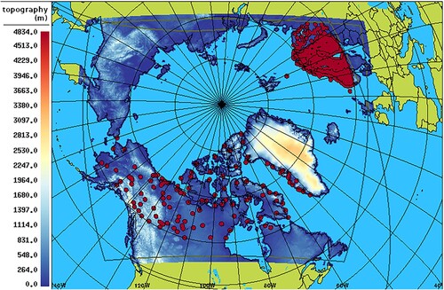
The initial and boundary conditions for CAPS atmospheric fields are downscaled from the 25-km GDPS (Buehner et al., 2015), which is coupled to GIOPS (G. C. Smith et al., 2016). While downscaling from the 10-km RDPS would have enabled a smaller resolution jump, the RDPS domain does not fully cover the CAPS and RIOPS domains (e.g. along the Euro-Asian coasts), therefore the GDPS was used. The uncoupled CAPS (prior to the 28th of June 2018) uses persisted sea-ice and ocean conditions, inherited from the coupled global prediction systems (3DVar ice analysis, Buehner et al., 2016; and CCMEP ice analysis, Brasnett, 2008). Since the 29th of June 2018, CAPS is fully coupled with RIOPS (Dupont et al., 2015; Lemieux et al., 2016), with initial ice-ocean conditions downscaled from GIOPS, using a spectral nudging method, and blended with a regional 3DVar ice analysis (Lemieux et al., 2016).

RIOPS uses the Nucleus for European Modeling of the Ocean (NEMO, Madec et al., 2008) model (version 3.1) and the Los Alamos Community Ice Code (CICE, Hunke & Lipscomb, 2010) version 4.0. The domain covers the Arctic Ocean and North Atlantic Ocean northwards of 26°N with a spatial resolution varying from 8 km in the south to 3 km in the Arctic. Additional details on the ice-ocean modelling components can be found in Dupont et al. (2015) and G. C. Smith et al. (2018, 2021).

Coupling between the NEMO-CICE ice-ocean model and GEM is made using the CCMEP coupler. Fluxes are calculated by NEMO and exchanged with GEM at every common model time-step (see G. C. Smith et al., 2018 for details on coupling methodology). Since the GEM and NEMO-CICE model grids are not aligned, a hybrid-approach is taken to calculate surface fluxes. For the part of the RIOPS domain in the North Atlantic Ocean that extends beyond the CAPS atmospheric domain, fluxes are calculated using surface atmospheric fields taken from the GDPS. Likewise, for the area in the North Pacific for which there is no RIOPS ocean model, the CAPS atmospheric component calculates fluxes using ocean surface conditions from GIOPS. The same flux routines are employed in both GEM and NEMO to ensure consistency.

For clouds and precipitation CAPS uses a “hot” start approach, where prognostic hydrometeor fields at the initial time-step come from the 12-hour forecast of the previous integration. CAPS uses the single-ice-category configuration of the Predicted Particle Properties (P3) microphysics scheme (Milbrandt & Morrison, 2016; Morrison & Milbrandt, 2015) to predict grid-scale clouds and precipitation. In the P3 scheme, all ice-phase hydrometeors (ice crystals, snow, graupel, etc.) are represented by a single “free” ice category, whose physical properties (e.g. density and fall speed) evolve continuously in time and space. Cloud droplets and rain are also explicitly prognosed (from which drizzle vs. rain and freezing vs. non-freezing can be diagnosed). Because P3 is a full and detailed microphysics scheme, CAPS captures the effects of hydrometeor drift (the horizontal advection of hydrometeors as they fall), which impacts the timing and location of precipitation at the surface. This is in contrast to the GDPS and RDPS which use the comparatively simple Sundqvist grid-scale condensation scheme with diagnostic precipitation (Pudykiewicz et al., 1992; Sundqvist, 1978). The benefits of representing hydrometeor drift in operational NWP systems that use P3 versus Sundqvist are examined in detail in Mo et al. (2019).

The land-surface scheme used in CAPS is the Interaction between Soil, Biosphere and Atmosphere (ISBA, Bélair, Brown, et al., 2003; Bélair, Crevier, et al., 2003; Noilhan & Planton, 1989). Upper-level boundary conditions (“lid-nesting”, McTaggart-Cowan et al., 2011) come from the GDPS.

3 Verification domains and statistics

The WMO CBS provides worldwide guidance to National Meteorological Centres, for the evaluation and international exchange of global model verification scores (WMO-485 manual). The verification domains, aggregation strategy and verification statistics considered in this study are partially inspired by these CBS directives.

The CBS standards recommend that surface variable scores are exchanged for all stations and aggregated over monthly periods, whereas upper-air variable scores are aggregated over predefined domains and evaluated daily. In this study, we assess the overall model performance aggregating surface variable scores both spatially and temporally (Sections 4 and 5). However, we show maps with individual station scores when analysing specific aspects (e.g. regionalisation and representativeness issues) of the model performance (Section 6).

Operational CBS exchange of global model verification scores for upper-air variables over the Arctic is performed over the whole North Pole domain, defined as all latitudes greater than 60^oN. In this study, however, we do not consider the whole North Pole domain for the following reasons:

1. While GDPS has global coverage, CAPS and RDPS do not cover the whole North Pole domain; in order to properly compare the three models, verification is limited to common sub-domains.

2. Several variables exhibit a diurnal cycle in their scores: such signal would be damped and hidden when considering a domain encompassing a too large range of longitudes.

3. Fennoscandia is characterised by a very dense network, which would dominate the scores for the whole North Pole Regions.

Verification is therefore performed over two sub-domains (Fig. 1): North America North (NAN), which includes 140 stations, and spans all latitudes greater than 60°N and longitudes between 170^oW and 50^oW, and Fennoscandia, which includes 497 stations, and spans the latitudes between 60^oN and 75^oN and longitudes between 0° and 40°E. Note that the NAN domain, despite being larger, is characterised by a smaller verification sample (both for stations and number of monthly recorded observations) than Fennoscandia; therefore, NAN verification statistics are noisier, their confidence intervals exhibit larger uncertainty, and the verification results are overall less robust.

Unless otherwise specified, verification is performed against the WMO synoptic observations that were available on the WMO Global Telecommunication System during the winter and summer SOPs and that were harvested by the CCMEP. As per the CBS directives (WMO-485 manual), solely observations from WMO white-listed stations, and solely observations not rejected by the in-house CCMEP data assimilation systems are used for verification. Station observations are paired with the nearest grid-point model value. Raw model output, with no post-processing or adjustment (unless specified), on the original model grid is considered.

Near-surface air temperature and dew-point temperature are verified using traditional continuous scores (Jolliffe & Stephenson, 2012, chapter 5). As summary of the model performance, we show the bias and error standard deviation (e.g. Figs. 2 and 4). When comparing the forecast (F) to the corresponding observations (O), the bias is the average of the errors (E = F-O), stratified for each individual lead-time and aggregated over the whole verification period and for all the stations within the verification domain. The error standard deviation is defined as: (1) $\mathrm{stdev}[E]=\sqrt{\mathrm{mean}[{(E-\mathrm{mean}[E])}^2]}=\sqrt{\mathrm{var}[E]}$(1) and is evaluated again for each individual lead-time, aggregating over the whole verification period and domain. The error standard deviation is often preferred over other accuracy measures since it assesses the model accuracy independently from the bias. In fact, since the Mean Square Error (MSE) can be written as: (2) $\mathrm{MSE}=\mathrm{mean}[E^2]=(\mathrm{mean}[E]{)}^2+\mathrm{mean}[{(E-\mathrm{mean}[E])}^2]=\mathrm{bia}{\mathrm{s}}^2+\mathrm{var}[E]$(2) then the error standard deviation is considered to be the un-biased component of the Root Mean Square Error (RMSE).

Precipitation was verified for 6-hour accumulations, with traditional categorical scores (Jolliffe & Stephenson, 2012, chapter 3) evaluated from the contingency table entries for fixed precipitation thresholds. Given that the Arctic is characterised by an arid climate, we show solely the 0.2 (trace), and 1 mm thresholds: results obtained for 2 mm or larger thresholds are qualitatively similar to those for 1 mm, but exhibit larger uncertainty and noisy behaviours due to the increasingly smaller sample. As summary performance measures we show the Frequency Bias Index (FBI), which is the ratio between the number of forecast and observed events, and the Threat Score (TS) and Heidke Skill Score (HSS) as measures of accuracy and skill. These are computed as: (3) $\mathrm{FBI}=(a+b)/(a+c)$(3) (4) $\mathrm{TS}=a/(a+b+c)$(4) (5) $\mathrm{HSS}=(a+d-a_r-d_r)/(a+b+c+d-a_r-d_r)$(5) where a, b, c and d are the hits, false alarms, misses and nils (correct rejections) estimated from the contingency table entries, and (6) $a_r=(a+b)(a+c)/(a+b+c+d)$(6) (7) $d_r=(d+b)(d+c)/(a+b+c+d)$(7) are the hits and nils that one would expect from random chance (see Jolliffe & Stephenson, 2012, chapter 3, for full explanation).

Wind is a circular vectorial variable, characterised by a magnitude (the wind speed) and a direction. To verify wind forecasts in an exhaustive fashion we verify:

1. The wind speed, by evaluating its bias and error standard deviation (as for the temperatures, these assess the accuracy separately from the bias).

2. The wind direction, by evaluating its Mean Absolute Error (MAE), i.e. the average of the absolute values of the difference (in degrees) between forecast and observed wind directions.

3. The wind overall performance is evaluated with the modulus ($||$) of the vectorial difference of the forecast ($\overrightarrow{f}$) and observed ($\overrightarrow{o}$) wind vectors: (8) $|\overrightarrow{e}|=\sqrt{{(f_x-o_x)}^2+{(f_y-o_y)}^2}$(8) where f_x, o_x and f_y, o_y are the x and y components of the forecast and observed wind vectors, respectively.

This latter score evaluated over the whole verification sample (for i = 1, … , n, where the index i represent the individual forecast-observation pair), (9) $\mathrm{VRMSE}=\sqrt{{\displaystyle \frac{1}{n}\sum _{i=1}^n[{(f_x^i-o_x^i)}^2+{(f_y^i-o_y^i)}^2]}}$(9) corresponds to the Root Mean Square of the modulo of the Error vectors $|\overrightarrow{e}|$, and it is therefore referred to as the vector RMSE. Note that the vector RMSE is sensitive to errors in both wind speed and wind direction. Moreover, the vectorial difference of two wind vectors with slightly offset directions tends to be larger for larger wind speeds; therefore, the vector RMSE implicitly penalises model errors for strong winds more severely.

The wind direction and wind vector RMSE are evaluated for observed wind speeds exceeding 3 m/s, to eliminate the noisy signal of weak winds (which usually do not have a well-defined direction). The CBS recommends this unilateral condition (applied solely to observed wind speeds), in order to compare models from different centres using the same observation dataset. In Section 4 we evaluate the wind direction and vector RMSE by also applying the bilateral condition, when both observed and forecast wind speed exceed 3 m/s, and we compare the results obtained.

Verification statistics are aggregated over all stations within the domains considered (Fennoscandia and North America North) during the two periods of February–March 2018 (winter SOP) and July-August-September 2018 (summer SOP). All statistics are stratified and shown in function of the forecast lead-time. Scores are evaluated with a frequency of 3 hours (6-hour accumulations for precipitation), up to the CAPS 48-hour lead-time (RDPS and GDPS run for longer lead-times, but since the scope of the article is to compare CAPS with the other Canadian deterministic prediction systems, we show solely the common lead-time). Scores are shown solely for the 00 UTC run: scores for the 12 UTC run behave very similarly and therefore are not shown.

Statistical significance of the performance difference between CAPS and RDPS, and between CAPS and GDPS is assessed by evaluating the 90% confidence intervals of the score difference, with a block bootstrapping technique of paired datasets (Efron & Tibshirani, 1993). Bootstrap methods involve a random selection of cases from the original (verification) dataset, to obtain a resample with a number of cases similar to that of the original data sample. If the random selection is performed with replacement, an individual case might be selected (and belong to the resample) multiple times, which enables a smoother approximation of the (aggregated score) distribution. In this study, a resampling with replacement was performed over all dates within the verification period, 5000 times, and aggregated scores were evaluated for each of the 5000 resamples. Blocks of 3 days were considered in the resampling, to reduce the effect of forecast performance autocorrelation within the verification-period time-series. In each re-sampling, the same pairs of forecast and observation over the same dates are sampled for the two models compared, to obtain paired aggregated scores. The 5000 differences of these paired aggregated scores constitute the distribution of score differences from which the 90% confidence intervals are evaluated.

4 Canadian deterministic prediction systems overall performance

a Summer Performance

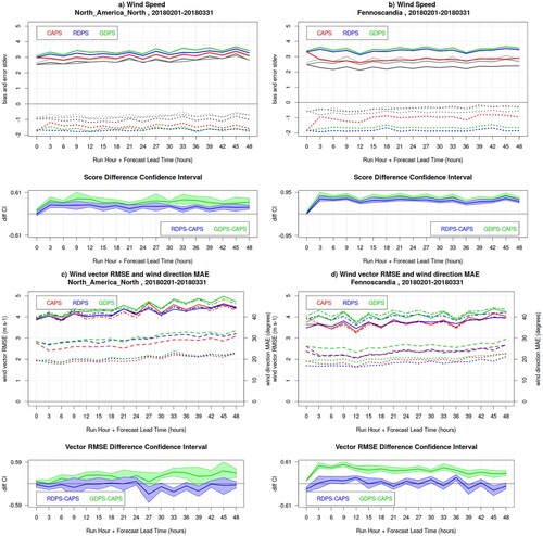
Figures 2 and 3 show the verification results for near-surface temperature, dew-point temperature and wind for the 00Z runs of CAPS, RDPS and GDPS, for the summer SOP, over North America North and Fennoscandia.

Fig. 2 Bias (dotted lines) and error standard deviation (solid lines) for near-surface air temperature (panels a and b) and dew-point temperature (panels c and d) for the 00Z runs of CAPS (red), RDPS (blue), GDPS (green) models, for the summer SOP, over North America North (left panels) and Fennoscandia (right panels). In the bottom sub-panels, the blue and green lines are the RDPS-CAPS and GDPS-CAPS score difference for the error standard deviation, with its associated bootstrap 90% confidence interval (blue and green shading): positive values indicate a statistically significant better score for CAPS.

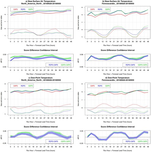
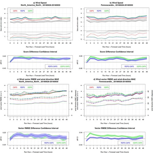
Fig. 3 Wind verification results for the 00Z runs of CAPS (red), RDPS (blue), GDPS (green) models, for the summer SOP, over North America North (left panels) and Fennoscandia (right panels). Panels a and b show the bias (dotted lines) and error standard deviation (solid lines) for wind speed; grey curves (dark for CAPS, medium for RDPS, light for GDPS) show the same statistics obtained solely for forecast and observed winds exceeding 3 m/s (bilateral condition). In the lower sub-panels, the blue and green lines are the RDPS-CAPS and GDPS-CAPS error standard deviation difference, with its associated bootstrap 90% confidence interval (blue and green shading): positive values indicate a statistically significant better score for CAPS. Panels c and d show the wind vector RMSE and the wind direction MAE (with scale values on the right vertical axis), when both forecast and observed wind speeds are larger than 3 m/s (solid and dotted lines, respectively), and when observed wind speeds (only) are larger than 3 m/s (dot-dashed and dashed lines, respectively). In the lower sub-panels, the blue and green lines are the RDPS-CAPS and GDPS-CAPS vector RMSE score difference for the statistics obtained with the bilateral condition, with its associated bootstrap 90% confidence interval (blue and green shading): positive values indicate a statistically significant better score for CAPS.

Summer near-surface air temperature biases (Fig. 2(a,b), dotted lines) over both domains exhibit a sinusoidal behaviour, with an overall negative sign and a strong diurnal cycle, with a maxima in the night and a minima in the day. The behaviour of the temperature bias is analysed in detail in Section 6. The diurnal cycle in the bias aligns with a systematic error in NWP systems, which have the tendency of not being able to reproduce the amplitude of the temperature diurnal cycle (they do not attain the daily minimum and maximum temperatures), so that night-time minima are too warm and day-time maxima are too cold. CAPS exhibits a smaller error (Fig. 2(a,b), solid lines), especially at night-time, compared to RDPS and GDPS, which is significant with 90% confidence (Fig. 2(a,b), lower sub-panels, green and blue shading).

Note that the bias curves for the NAN domain compared to those for Fennoscandia are shifted in their phase by approximately 9 hours, due to the time zone difference between the two regions (in Fennoscandia the night-time minimum temperature occurs around 0:00–3:00 UTC, whereas in North America the night-time minimum occurs around 9:00–12:00 UTC). Moreover, the amplitude of the bias diurnal cycle is possibly more pronounced for Fennoscandia, because its domain spans only 40 degrees longitude, as opposed to the 120 degrees longitudes spanned by the NAN domain (on the NAN domain the bias diurnal cycle is damped while aggregating a larger range of longitudes).

Summer dew-point temperatures (Fig. 2(c,d)) exhibit also a sinusoidal behaviour, with an overall negative bias for RDPS and GDPS (the models are too dry), a positive bias for CAPS (the model is too humid), and a diurnal cycle opposite to that of the air temperature, indicating models more humid (less dry) during the day and more dry (less humid) during the night. CAPS exhibits a significantly better bias and a significantly smaller error at night-time, compared to RDPS and GDPS (again with 90% confidence).

Summer wind speeds are underestimated (Fig. 3(a,b), dotted lines) and the bias exhibits a diurnal cycle, with stronger underestimation during the day (whereas during the night the models are more windy). RDPS and GDPS are systematically less windy than CAPS. CAPS exhibits a significantly smaller error in wind speed (Fig. 3(a,b), solid lines), compared to RDPS and GDPS. When considering solely forecast and observed wind speeds exceeding 3 m/s (grey lines), both bias and error are reduced, indicating that a large portion of the error is attributed to weak winds. For wind direction and overall wind prediction (as assessed by the vector RMSE) CAPS exhibits better or comparable performance to the RDPS and GDPS.

When assessing the wind direction (Fig. 3(c,d), dotted and dashed lines), the bilateral condition (observed and forecast wind speed greater than 3 m/s) exhibits better wind direction performance than the unilateral condition (observed wind speed greater than 3 m/s). While sustained winds (greater than 3 m/s) have smaller directional errors, the performance assessed applying solely the unilateral condition is worsened because dominated by a large number of directional errors of weak forecast winds. The vector RMSE (Fig. 3(c,d), dash-dotted and solid lines) is less affected when applying the bilateral versus unilateral condition, since the score is by definition not strongly affected by errors associated to weak winds. The score differences and ranking between the models slightly change when applying the unilateral versus bilateral condition.

The summer scores often cluster model behaviours, with CAPS on one side and RDPS and GDPS on the other: CAPS outperforms the two other models for temperature, dew-point temperature, and wind representation, over both domains. The 12Z runs exhibit a very similar behaviour and therefore are not shown.

b Winter Performance

Figures 4 and 5 show the verification results for near-surface temperature, dew-point temperature and wind for the 00Z runs of CAPS, RDPS and GDPS, for the winter SOP, over North America North and Fennoscandia. Winter verification results are consistent with summer results.

Fig. 4 Bias (dotted lines) and error standard deviation (solid lines) for near-surface air temperature (panels a and b) and dew-point temperature (panels c and d) for the 00Z runs of CAPS (red), RDPS (blue), GDPS (green) models, for the winter SOP, over North America North (left panels) and Fennoscandia (right panels). For Fennoscandia, the error standard deviation for February-March 2019 (dot-dashed lines) and 2020 (dashed lines) is also illustrated. In the bottom sub-panels, the blue and green lines are the RDPS-CAPS and GDPS-CAPS score difference for the error standard deviation, with its associated bootstrap 90% confidence interval (blue and green shading): positive values indicate a statistically significant better score for CAPS.

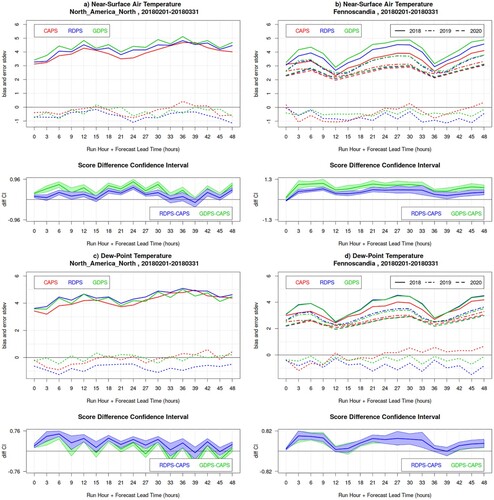
Fig. 5 As Figure 3, but for the winter SOP.

As in the summer, winter near-surface air temperature bias (Fig. 4 (a,b), dotted lines) exhibits an overall negative sign and a diurnal cycle with a maxima in the night and a minima in the day (as if the models do not attain the maxima and minima of the temperature diurnal cycle, on top of an overall cold bias). CAPS exhibits a significantly smaller error (Fig. 4(a,b), solid lines) compared to RDPS and GDPS, especially during the night for Fennoscandia.

Winter dew-point temperature bias (Fig. 4(c,d), dotted lines) exhibits a less remarkable diurnal cycle than for the summer bias. RDPS exhibits an overall negative bias (too dry), the GDPS is less dry and attains neutral bias in the NAN domain, while CAPS exhibits an increase in humidity with lead-time, switching from negative to positive bias. CAPS exhibits an overall significantly smaller error compared to RDPS and GDPS (with 90% confidence), especially during night-time for Fennoscandia.

The temperature error standard deviations for February–March 2019 and 2020 are also shown in Fig. 4, for Fennoscandia. All three models exhibit improvement with time, which mirrors the steady advancements of operational NWP systems (Bauer et al., 2015). GDPS and RDPS had two major implementations in September 2018 and July 2019 (McTaggart-Cowan et al., 2019; Separovic et al., 2019; see also the ECCC-MSC website https://eccc-msc.github.io/open-data/msc-data/changelog_nwp_en/ hosting the history of the Canadian models and their updates), which are reflected in an important error reduction (the two coarse-resolution models approach the performance of the high-resolution model in winter 2020). CAPS exhibits an important error reduction from winter 2018, when it was still uncoupled, to 2019, when it was coupled with RIOPS: this shows the added value of coupling. On the other hand, 2019–2020 exhibits a smaller jump in performance, since no major changes were performed into CAPS in that time period. Improvements over NAN are similar to those in Fennoscandia, but with scores less neatly separated, and hence are not shown.

Winter wind speed (Fig. 5(a,b), dotted lines) is again underpredicted and exhibits a very mild diurnal cycle (less remarkable than for the summer). Again, RDPS and GDPS are systematically more biased than CAPS, and CAPS exhibits a significantly smaller error in wind speed (Fig. 5(a,b), solid lines). When applying the bilateral condition (grey lines), both bias and error are reduced, indicating again that weak winds are associated with a large portion of the forecast error. As for the summer, the MAE for wind direction and the vector RMSE show that CAPS exhibits similar or better performance than the RDPS and GDPS. Again, applying the bilateral condition reduce remarkably the error in wind direction (otherwise dominated by the large number of directional errors associated with weak forecast winds), while the vector RMSE is less affected.

c Effects of the Sample Size on Verification Results

Table 1 lists the sample size of the measurements associated with the temperature and wind summary statistics shown in Figs. 2–5. Fennoscandia has a larger number of measurements than the NAN domain, of approximately a factor of 4. The number of summer measurements is approximately double than the number of winter measurements. Wind measurements are half than temperature measurements and applying the bilateral condition (e.g. for scoring the wind direction) further diminish the sample size. The different sample sizes are reflected in the width of the confidence intervals (blue and green shading in Figs. 2–5), which are generally larger for winter versus summer, for NAN versus Fennoscandia, for winds versus temperatures.

Table 1. Measurement sample sizes associated with the temperature and wind summary statistics shown in Figures 2–5. The wind direction reduced sample includes solely cases when both observed and forecast winds are stronger than 3 m/s.

	North America North	Fennoscandia
Temperature summer	10,600	44,000
Temperature winter	6,600	28,400
Wind speed summer	6,600	19,600
Wind speed winter	2,900	9,700
Wind direction summer	3,800	10,000
Wind direction winter	1,500	4,800

Surface synoptic observations exhibit slightly more reports for 00, 06, 12, 18 UTC than for 03, 09, 15, 21 UTC, which results in a saw-tooth behaviour of some scores (e.g. Fig. 4(a,c), and Fig. 5), which is more pronounced when the sample size is small (e.g. in winter, for NAN, for the winds). The change in the sampled stations affects the results because of the change in geographical coverage (the station network does not represent nor sample homogeneously the full geographical domain). There are slightly less synoptic observations in the evening and at night-time (over both domains), with mild effects on the summary statistics.

For wind direction and the wind vector RMSE (Figs. 3 and 5, panels c and d), the bi-lateral condition of observed and forecast winds stronger than 3 m/s was used in the verification (in order to filter out the possibly misleading signal of weak winds). Statistics were therefore computed over a reduced sample size (last two rows of Table 1). The sample size for winds exceeding 3 m/s has a strong diurnal cycle, with fewer events during the night. This, combined with the smaller number of night-time synoptic records, results in a more noisy signal of the wind scores at night-time (e.g. Figs. 3 and 5, panels a and c) over the NAN domain (which has a smaller sample size to start with).

For some statistics in Figures 2–5, there is a jump from 0 to 3-hour lead-time, which is due to the CAPS initialisation (downscaling) from the GDPS and subsequent spin-up.

5 Precipitation

a NWP Precipitation Overestimation

Precipitation accumulated over 6 hours was verified against observations from two station networks: the synoptic network used for reporting surface observations from land-based stations, either staffed or automatic (ECCC-MANOBS, 2019), and the station network assimilated into the Canadian Precipitation Analysis (CaPA, Fortin et al., 2018), which includes the synoptic stations and other regional networks, such as the stations of Hydro-Quebec. Precipitation was verified with traditional categorical scores evaluated from the contingency table entries for fixed precipitation thresholds.

For summer precipitation (Fig. 6), CAPS exhibits nearly no bias for small thresholds (0.2 mm) and a positive bias (FBI approximately 1.2) for larger thresholds. RDPS and GDPS exhibits larger positive biases (FBI approximately 1.3–1.4) than CAPS, for all lead-times and thresholds, and on both verification domains. The three models exhibit similar accuracy (in terms of TS, not shown) and skill (in terms of HSS) for all lead-times and on both verification domains (with RDPS and GDPS marginally better than CAPS for 1 and 2 mm thresholds).

Fig. 6 Frequency Bias Index (FBI) and Heidke Skill Score (HSS) of the CAPS (red) RDPS (blue) and GDPS (green) models, evaluated against precipitation measurements of the CaPA station network, for 6 h precipitation accumulation exceeding 0.2 mm (left column panels), 1.0 mm (central column panels) and 2.0 mm (right column panels), for Fennoscandia and North America North, during the summer SOP.

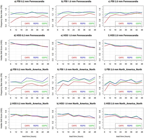
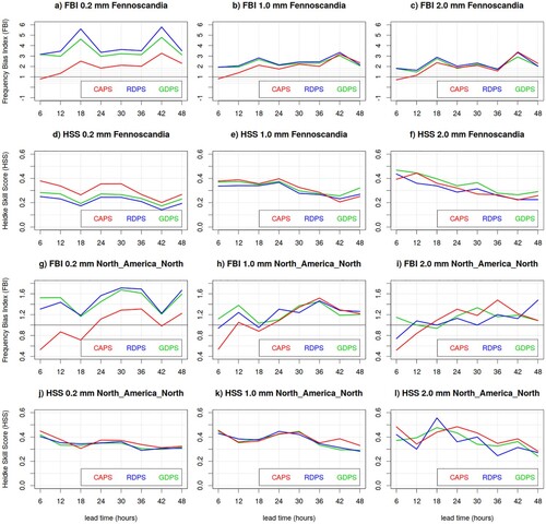
For winter precipitation (Fig. 7), CAPS exhibits a smaller bias and better skill (over Fennoscandia) than RDPS and GPDS for small thresholds (0.2 mm). For higher thresholds, the three models exhibit similar accuracy and skill and a positive bias (marginally better for CAPS), for all lead-times and thresholds, and over both verification domains. The particularly large positive bias over Fennoscandia is due to the solid precipitation undercatch (possibly enhanced over Fennoscandia due to the larger sample size with respect to the NAN domain), which is explained and addressed in Sections 5.2 and 5.3.

Fig. 7 Frequency Bias Index (FBI) and Heidke Skill Score (HSS) of the CAPS (red) RDPS (blue) and GDPS (green) models, evaluated against precipitation measurements of the CaPA station network, for 6 h precipitation accumulation exceeding 0.2 mm (left column panels), 1.0 mm (central column panels) and 2.0 mm (right column panels), for Fennoscandia and North America North, during the winter SOP.

Coarse resolution models, such as RDPS and GDPS, are often affected by the overestimation of trace precipitation (i.e. precipitation amount of less than 0.1 mm). This is partially due to the lack of precipitation trace recording in station measurements, and partially due to a representativeness issue: since their coarse resolution does not allow representation of small-scale precipitation events, the water equivalent is spread over the entire model tile, producing a trace signal. The better performance of CAPS for small thresholds is partially due to its finer resolution. In addition, the P3 microphysics in CAPS allows for hydrometeor drift, thus light precipitation, which sediments slowly, can be transported horizontally before reaching the surface. A better timing and location of light precipitation can then possibly contribute to a more accurate prediction. CAPS (and sometimes RDPS) bias in the initial lead-times is drier than for the overall forecast run, due to the precipitation spin-up.

b Solid Precipitation Undercatch and Operational Quality Controls

Precipitation measurements from standard instrumentation at synoptic stations are affected by the undercatch of solid precipitation in windy conditions. Kochendorfer et al. (2017) estimated a 24% undercatch for Single Alter gauges, and a 34% undercatch for unshielded gauges. This represents a severe problem for precipitation forecast verification, especially at high latitudes and in winter, since the undercatch might artificially inflate the NWP precipitation overestimation.

Quality control of NWP verification systems often flags solid precipitation measurements in windy conditions, so that they do not get included in the calculation of verification scores. However, the removal of solid precipitation measurements by quality control procedures leads to an important reduction of the verification sample size. This can result in giving more weight to wind-sheltered regions. Moreover, this selective quality control systematically eliminates major snow events (which usually occur under windy conditions).

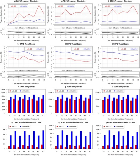
We quantify the effects of the quality controls verifying the Canadian NWP systems against precipitation measurements of the CaPA network (Fig. 8). For Fennoscandia in February–March 2018, the verification sample size is reduced by 20% (Fig. 8, panels c, g and k), and the precipitation events are reduced by over 80% (Fig. 8, panels d, h and l): this indicates that in the 20% of the verification sample rejected by the quality control, 80% of the precipitation events occurred. The verification results are significantly affected by the selective quality control. As expected (since quality control removes observed snow events), frequency bias against quality-controlled measurements exhibits a larger over-forecast than frequency bias against not quality-controlled measurements (Fig. 8, panels a, e and i). The threat score against quality-controlled measurements exhibits worse performance than against non-quality-controlled measurements (Fig. 8, panels b, f and j), due to the elimination of most of the hit events (occurring during the major snow storms) from the verification sample. Also miss events are removed from the verification samples, but in lesser proportion than the hits, and the forecast performance thus becomes dominated by the false alarms (which are not affected by this quality control procedure).

Fig. 8 Frequency Bias Index (top row panels a, e and i), Threat Score (second row panels b, f and j), verification sample size (third row panels c, g and k) and base rate (number of observed events exceeding the 1 mm threshold, bottom row panels d, h and l) evaluated against precipitation measurements of the CaPA station network, for 6 h precipitation accumulation exceeding 1.0 mm, for the CAPS (left panels), RDPS (central panels) and GDPS (right panels) in Fennoscandia during the winter SOP. In each graph, red curves and bars are obtained from quality controlled data (with QC), whereas blue curves and bars are obtained from non-quality controlled data (without QC); the lower sub-panels of a, b, e, f, i and j show the score difference (black line) with its associated bootstrap 90% confidence interval (grey shading).

For North America North again in February–March 2018 (not shown), the scores for quality-controlled against non-quality-controlled precipitation measurements exhibit a similar behaviour as Fennoscandia (smaller over-forecast and better performance for non-quality controlled measurements), but the effects were less important, possibly due to the smaller verification sample available for the NAN domain.

c Adjustment for Solid Precipitation Undercatch

The WMO Solid Precipitation Inter-Comparison Experiment (SPICE) has performed a multi-site inter-comparison and evaluation of instruments for measuring solid precipitation. Comparison with Double Fence Automated Reference installations enabled the quantification of the undercatch. The WMO-SPICE report (Nitu et al., 2018), and Kochendorfer et al. (2017, 2018) provide recommendations for adjustment functions to correct the solid precipitation undercatch under windy conditions.

In this work, we adjust the solid precipitation undercatch by dividing the observed measurements with the Catch Efficiency (CE), evaluated following Kochendorfer et al. (2017), Eq. (3): (10) $\mathrm{CE}=e^{[-a\cdot UV\cdot (1-{\tan }^{-1}(b\cdot TT)+c)]}$(10) where UV is the wind speed, TT is the air temperature, and the parameters a, b and c are estimated parameters which depends on the wind shield of the installation, the height of the wind measurements (gauge height or 10 m), and the local climatology of the station. Adjustments for wind speeds beyond a threshold th are kept constant because the increasingly smaller sample size with increasing UV thresholding did not permit a sufficiently reliable estimation (J. Kochendorfer, personal communication, June 2020).

Figure 9(a) shows the CE theoretical curve for the universal parameters a, b, c, and th estimated by Kochendorfer et al. (2017), aggregating results for several WMO-SPICE locations. The catch efficiency depends on the type of gauge and height of wind measurements: as expected, catch efficiency for Single Alter shielded gauges is better than for unshielded gauges (the CE curve for Single Alter shielding is nearer to one). Similarly, the adjustment for 10 m winds is smaller than for gauge-height winds. The shielding characteristics have more impact on the catch efficiency than the height of the wind measurements.

Fig. 9 Solid precipitation undercatch adjustment function proposed by Kochendorfer et al. (2017), where the Catch Efficiency (y-axis) is plotted as function of wind speed (x-axis). The top panel shows the Universal adjustment for different gauge shields and heights of wind measurements, whereas the bottom panel compares the adjustments for different locations and temperatures, for installations with Single Alter shielding and wind measurements at 10 m. The circles in the top panel and vertical lines in the bottom panel correspond to the wind speed thresholds beyond which the adjustment is kept constant.

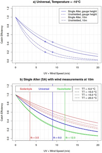
Figure 9(b) shows the CE theoretical curves for Single Alter shielded installations with wind measurements at 10 m, which is the most common setting at the synoptic stations, for different temperatures. Along with the universal adjustment, we also show the catch efficiency for Sodankyla (Finland) and Haukeliseter (Norway), which are two of the WMO-SPICE sites located in Arctic environment. The parameters a, b, c, and th estimated for these two locations were provided by E. Mekis and J. Kochendorfer (personal communication, June 2020) and are shown in Table 2. Sodankyla is characterised by a forested (naturally shielded) environment, hence a milder adjustment. Haukeliseter, on the other hand, is located in mountain terrain with a very windy climatology, therefore, it is characterised by a stronger adjustment. Sodankyla’s adjustment is more temperature-dependent than Haukeliseter adjustment. Given that the typical instrument errors for temperature are 0.1°C and for wind are 0.5 m/s, Figure 9(b) shows that the local climatology has a stronger impact on the adjustment (the curves for the different sites are well separated), than the temperature and wind measurement uncertainty.

Table 2. Estimates of the parameters a, b and c and threshold th associated with the catch efficiency for installations with Single Alter (SA) versus unshielded (Un) gauges, with 10 m versus gauge-height (gh) wind measurements, used to obtain the Universal, Sodankyla and Haukeliseter adjustment function.

Parameter	Installation type	Universal	Sodankyla	Haukeliseter
a	SA, 10m	0.0281	0.04005	0.05068
a	SA, gh	0.0348	0.05421	0.05450
a	Un, 10m	0.0623	0.09763	0.07138
a	Un, gh	0.0785	0.13210	0.07675
b	SA, 10m	1.628	0.06113	0.9753
b	SA, gh	1.366	0.06096	0.9753
b	Un, 10m	0.776	0.05700	1.0930
b	Un, gh	0.729	0.05699	1.0930
c	SA, 10m	0.837	0.00000000029	0.3435
c	SA, gh	0.779	0.00000029700	0.3435
c	Un, 10m	0.431	0.00000533700	0.4591
c	Un, gh	0.407	0.00000229600	0.4590
th	SA, 10m	9.0	3.5	12.0
th	SA, gh	7.2	3.0	9.0
th	Un, 10m	9.0	3.5	12.0
th	Un, gh	7.2	3.0	9.0

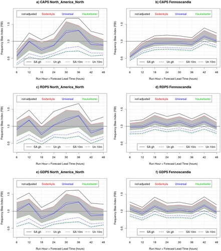
Figure 10 shows the 6-hour accumulated precipitation FBI for 1 mm threshold, evaluated against the adjusted solid precipitation measurements from the synoptic station network, for CAPS, RDPS and GDPS over North America North and Fennoscandia during the winter SOP. The NWP systematic positive bias for winter precipitation is significantly reduced when considering adjusted measurements. For the synoptic network we consider Single Alter shielding with 10 m wind measurements the most suitable adjustment (dotted lines in Fig. 10), since this is the most common type of installation at synoptic stations. The universal Single Alter 10 m adjustment leads to a neutral bias, with an uncertainty spanning from over- to under- forecast (grey shading in Fig. 10), depending on the station climatology. The FBI could, however, become negative if more aggressive adjustments would be considered (e.g. for unshielded gauges and/or extremely windy climatologies, such as in Haukeliseter).

Fig. 10 Frequency Bias Index for the CAPS (top panels) RDPS (central panels) and GDPS (bottom panels) model, evaluated against precipitation measurements of the synoptic station network, for 6 h precipitation accumulation exceeding 1.0 mm, over North America North (left column panels) and Fennoscandia (right column panels), during the winter SOP. The black curve is obtained against unadjusted measurements, whereas colour curves are obtained against adjusted solid precipitation measurements for Single Alter (SA) versus unshielded (Un) gauges, with 10 m versus gauge-height (gh) wind measurements, and applying the universal (blue lines), Sodankyla (red lines) or Haukeliseter (green lines) adjustment function.

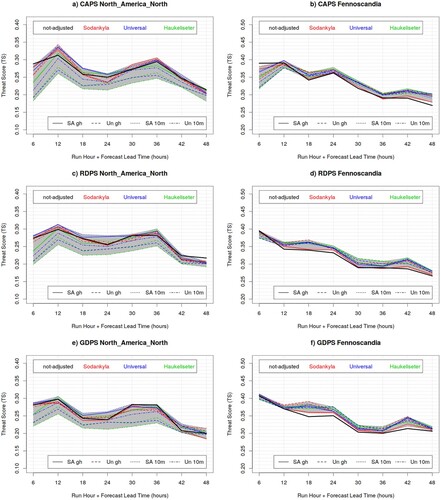
Figure 11 shows the 6-hour accumulated precipitation Threat Score for 1 mm threshold, evaluated against the adjusted solid precipitation measurements from the synoptic station network, for CAPS, RDPS and GDPS over North America North and Fennoscandia during the winter SOP. Over Fennoscandia the TS against the adjusted solid precipitation measurements is better than that evaluated against non-adjusted measurements (black thick line); stronger adjustments (e.g. Haukeliseter green curves) lead to a better performance than weak adjustments (e.g. Sodankyla red curve). Over the NAN domain, on the other hand, the adjustments do not lead to a consistent improvement. This might be related to the use of a unique adjustment for manned versus automated stations. Strong adjustments are associated with a poorer performance, and solely the universal adjustment consistently improve (mostly day-time) performance over the NAN domain.

Fig. 11 Threat Score for the CAPS (top panels) RDPS (central panels) and GDPS (bottom panels) model, evaluated against precipitation measurements of the synoptic station network, for 6 h precipitation accumulation exceeding 1.0 mm, over North America North (left column panels) and Fennoscandia (right column panels), during the winter SOP. The black curve is obtained against unadjusted measurements, whereas colour curves are obtained against adjusted solid precipitation measurements for Single Alter (SA) versus unshielded (Un) gauges, with 10 m versus gauge-height (gh) wind measurements, and applying the universal (blue lines), Sodankyla (red lines) or Haukeliseter (green lines) adjustment function.

The span associated with the adjustment in Figures 10 and 11 is large, and ought to be considered an overestimated uncertainty. Here a unique adjustment was applied at all stations, as preliminary study to quantify the adjustment effects and associated uncertainty. Future work at ECCC will apply individual adjustments for individual stations, according to each station climatology and instalment characteristics, both for verification practices and for data assimilation into the CaPA analysis (Franck Lespinas, personal communication, June 2020).

6 Temperature lapse-rate adjustment

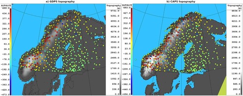
Gridded models cannot always fully resolve the complex topography associated with complex mountain terrains (Fig. 12). Model tiles in mountain terrains are often situated at a higher elevation than observing stations, which are typically located in the valleys. This leads to an enhanced NWP cold bias for surface temperatures (consistently with our findings in Section 4), since model tiles represent temperatures at (often glacier capped) mountain tops, whereas observations are taken in warmer valleys at lower elevation.

Fig. 12 (left) GDPS and (right) CAPS topography (grey shading, metres) over Fennoscandia, and altitude difference between the model topography and station elevations (colour dots, metres).

Temperature in a standard atmosphere decreases with altitude with a lapse-rate of approximately 0.0065°C/m. The CBS standards for verification of surface variables, therefore, recommend adjusting model tile temperature to the verifying station elevation by applying this lapse-rate adjustment (WMO-485 manual, Appendix 2.2.34). We tested this lapse-rate adjustment over the Fennoscandia domain.

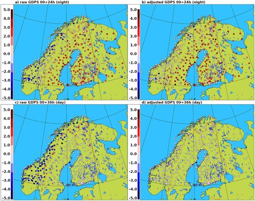
Figure 13 shows the maps of GDPS surface temperature bias, for the summer SOP over Fennoscandia, valid at 24 and 36 UTC (night-time and day-time respectively), before and after the model tile temperature adjustment to station elevation. The cold bias characterising the Norwegian mountain terrain is significantly reduced when applying the lapse-rate adjustment, both for day and night temperatures.

Fig. 13 GDPS surface temperature bias, for the summer SOP over Fennoscandia, at 24 and 36 UTC (night-time and day-time respectively), before and after the model tile temperature adjustment to station elevation.

Figure 14 shows the GDPS surface temperature bias, error standard deviation and RMSE as a function of lead-time, again for the summer SOP over Fennoscandia, before and after the temperature lapse-rate adjustment. The temperature-adjusted bias curves are higher for all lead-times, indicating a systematic warming of the model temperatures due to the adjustment (i.e. stations are on average at a lower elevation than model tiles). The bias is improved (is less cold) during the day but deteriorates (it is too warm) during the night. The error standard deviation improves systematically, for all lead-times. The RMSE, on the other hand, shows significant improvement solely for day-time adjustments, whereas during the night it exhibits mild to no improvement, mainly due to the too warm night-time bias.

Fig. 14 GDPS surface temperature RMSE (panel a), bias and error standard deviation (panel b, dotted and solid lines, respectively) as function of lead-time (x-axis), for the summer SOP over Fennoscandia, before (red and green curves) and after (blue and grey curves) the temperature lapse-rate adjustment. Statistics evaluated over the subset “altdiffmax500” of stations which differ at the most 500 m in altitude from the corresponding (nearest) model tile elevation are labelled “500” (blue and green curves). The bottom panel shows the difference between error standard deviations (grey) and RMSE (magenta) for the GDPS raw model output (red curves) versus the GDPS adjusted temperatures for tiles within 500 m from the station altitude (blue curves), with their associated bootstrap 90% confidence interval (grey and pink shading): negative values indicates a statistically significant better score for lapse-rate adjusted temperatures evaluated over the “altdiffmax500” subset of stations.

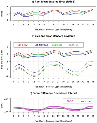
It is worth noting that the systematic improvement of the error standard deviation is due to the spatial aggregation of a more homogeneous error across the verification domain. In fact, the lapse-rate adjustment performs a bias correction which is constant for each individual station. Therefore, the error standard deviation for the individual stations does not change (not shown) because the standard deviation is invariant with respect to any additive constant, and therefore insensitive to the bias. However, when aggregating over the whole domain the error standard deviation improves because the lapse-rate adjustment, while decreasing the mountain station bias, renders the error geographically more homogeneous. For this reason, we show the RMSE along with the error standard deviation, when discussing the effects of the lapse-rate adjustment.

Figure 14 shows both statistics aggregated over all stations, and statistics for the subset of stations which differ by at most 500 m in altitude from the corresponding (nearest) model tile elevation. We label this subset of stations as “altdiffmax500” (sample size was reduced from approximately 45,000 to approximately 43,000 events). We analyse the behaviour of the verification statistics evaluated on this subset to determine if it is desirable to apply the temperature lapse-rate adjustment up to a maximum altitude difference (e.g. 500 m) between station and model tile. Prior to adjustment, the statistics differ significantly (green versus red curves), indicating that stations which are located at an altitude considerably different from the model tile elevation (larger than 500 m) contribute significantly to the model error. After applying the temperature lapse-rate adjustment (blue versus grey curves), on the other hand, the verification statistics evaluated over all stations do not differ significantly from those evaluated over the altdiffmax500 station subset. This result strengthens confidence in the lapse-rate adjustment and suggests there is no strong need to limit a model-tile versus station altitude difference.

The enhancement of the night-time warm bias by the lapse-rate adjustment might be partially due to the presence of temperature inversions, which often occur in clear and still nights. In these cases, temperatures in the valleys are colder than those at higher elevations, and the standard lapse-rate adjustment, instead of correcting the model tile representation, inflates the forecast error towards a warm bias. We, therefore, performed an additional experiment to test the behaviour of the verification statistics under inversion conditions.

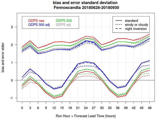
Figure 15 shows the GDPS surface temperature bias and error standard deviation evaluated over all stations with wind and cloud measurements (solid lines), for the summer SOP over Fennoscandia. The verification sample size was reduced from 45,000 to 36,000 events (from 43,000 to 34,000 for the altdiffmax500 subset), but the behaviour of the statistics is similar to that over the whole station network (Fig. 14). For these stations, we re-evaluate the verification statistics considering solely events with either some clouds (observed cloud cover greater than 1 okta) or some wind (observed wind speed greater than or equal to 3 m/s), in order to exclude many inversion cases. (The verification sample for inversion conditions exhibits a diurnal cycle with a maximum of approximately 4000 events at night, and a minima of 2000 events during the day). The verification statistics evaluated excluding inversion conditions (dotted lines) show better performance, especially at night, reinforcing our hypothesis that a large portion of the model error is associated with night-time inversion conditions. We then apply a lapse-rate adjustment with an inversion lapse-rate of −0.0032°C/m for the night temperatures (21, 24, 27 UTC; 18 and 30 UTC use a 0 lapse-rate as transition from the standard to the inversion lapse-rate) when inversion conditions are observed (observed cloud cover smaller than or equal to 1 okta and observed wind speed less than 3 m/s), for stations with elevation lower than the corresponding model tile. There is a very mild improvement in the statistics (dashed lines), which, however, does not explain all model error associated with inversions (estimated by the difference between the solid and dotted curves). A more in-depth analysis on the temperature vertical profiles and night inversions might help address this gap.

Fig. 15 GDPS surface temperature bias (lower curves) and error standard deviation (upper curves) as function of lead-time (x-axis), for the summer SOP over Fennoscandia. Solid lines show verification statistics evaluated over all stations with wind and cloud measurements; dotted lines show verification statistics evaluated excluding events with inversion conditions. Green and blue curves are evaluated over the subset “altdiffmax500” of stations which differ at the most 500 m in altitude from the corresponding (nearest) model tile elevation. Red and green curves are obtained against raw model output, whereas blue and grey curves are obtained by applying a temperature lapse-rate adjustment. Dashed blue curves are obtained applying a temperature adjustment with inversion lapse-rate of −0.0032°C/m when night-time inversion conditions occurred.

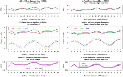
Figure 16 shows the Canadian deterministic prediction systems verification, again evaluated over all stations with wind and cloud measurements, for the summer SOP over Fennoscandia, before and after the model tile temperature adjustment to station elevation. The lapse-rate adjustment changes the ranking of the models: prior to adjustment, the higher resolution CAPS outperforms the coarser RDPS and GDPS. After applying the temperature lapse-rate adjustment (with night inversions), on the other hand, RDPS and GDPS score significantly better than CAPS during the day, and CAPS outperforms the coarser models solely during the night.

Fig. 16 Surface temperature RMSE (panels a and d), bias and error standard deviation (dotted and solid lines, respectively, in panels b and e), for the CAPS (red), GDPS (green) and RDPS (blue) as function of lead-time (x-axis), during the summer SOP over Fennoscandia. Verification statistics are evaluated over all stations with wind and cloud measurements: the left panels show results for raw model output, whereas the right panel shows results obtained after applying the temperature lapse-rate adjustment (with night inversions). The bottom panels shows the difference between the CAPS and GDPS error standard deviations (grey) and RMSE (magenta), with their associated bootstrap 90% confidence interval (grey and pink shading): positive values indicates a statistically significant better score for CAPS.

Lapse-rate adjustments of winter temperatures lead to very similar results as the ones shown for the summer temperature, just slightly less remarkable (and therefore they are not shown).

7 Discussion and conclusions

This work presents objective verification for near-surface variables (temperature, dew-point temperature, wind and precipitation) for the three Canadian deterministic NWP systems running operationally at the CCMEP during YOPP: the 25-km GDPS, the 10-km RDPS, and the 3-km CAPS, which was developed by the ECCC Meteorological Research Division explicitly for the WMO PPP/YOPP project. The verification covers the YOPP Arctic SOPs (Feb-March and July-Aug-Sept 2018). Verification methodology follows (and expands) the CBS directives for surface variables (WMO-485 manual).

Routine verification shows that overall CAPS outperforms RDPS and GDPS in predicting near-surface temperature, dew-point temperature, wind and precipitation, in both seasons and verification domains. All three systems exhibit a diurnal cycle in the near-surface temperature biases, with maxima at night and minima during the day. This systematic behaviour is found also in other NWP and climate models, which tend to underestimate the diurnal temperature range (Flato et al., 2013; Mearns et al., 1995). All three systems underestimate the wind speed, however, as weak winds are excluded from the verification sample bias and error are reduced substantially. All the three models have undergone some significant operational upgrades in the past two years: we illustrate that every major implementation corresponds to a jump in the performance statistics (e.g. for winter temperatures) and CAPS exhibits its major improvement when changing from uncoupled to a coupled system with RIOPS. Finally, all three systems seem to systematically over-predict precipitation; CAPS performs marginally better than the other two coarser resolution models and exhibits almost neutral bias for light precipitation.

Analysing more in-depth the precipitation over-prediction, we found that the NWP systems’ systematic over-forecast of winter precipitation at high latitude is artificially inflated by the wind-induced undercatch of solid precipitation measurements. To mitigate the effects of the solid precipitation undercatch, we apply the WMO-SPICE adjustment function provided by Kochendorfer et al. (2017) prior to verification. The Canadian NWP systems over-forecast is reduced, to attain neutral bias, after the adjustment.

Operational quality control flags solid precipitation measurements in windy conditions (rather than adjusting them) and removes them from the verification sample prior to the calculation of verification scores. This selective screening eliminates major snowstorms and reduces dramatically the sampled precipitation events (up to 80% of reduction), which significantly alters the verification results (Section 5.2). Our recommendation for operational environments is to adjust the solid precipitation measurements, rather than remove the observations from the verification sample.

There is a large uncertainty associated with the WMO-SPICE adjustment, which translates into uncertainty associated with the verification results against adjusted precipitation (Section 5.3). The largest source of uncertainty is associated with the local characteristics of the individual stations, and ideally adjustments should be adapted to these local climatologies. Future work at ECCC will apply individual adjustments for individual stations, both for data assimilation into the CaPA analysis, and for ECCC routine operational verification. We consider verification against the adjusted precipitation more reliable and informative than against the unadjusted and quality controlled (removed) precipitation. While individual station adjustments are being developed, the universal adjustment applied to the whole network provides possibly a better bias estimate, since the under- and over- adjustments (as shown by the Haukeliseter and Sodankyla stations) compensate when applied to a large network encompassing several stations with different installations and climatologies.

The undercatch is sensitive to the different types of hydrometeors, their shape and their microphysics (e.g. particle fall velocity is different if we consider snowflakes versus partially melted snow, or ice pellets). In the WMO-SPICE adjustment function used in this study this is possibly reflected in the temperature dependence of the adjustment and the different adjustments used for different locations characterised by different climatologies (where different hydrometeors might be the most recurring hydrometeors). Transfer functions dependent on precipitation intensity have been recently developed (Colli et al., 2020). Future research could evolve towards analysing the behaviour of the adjustment function stratifying for different hydrometeors (rather than locations). The use of numerical models that explicitly represent the hydrometeor microphysics (including shape, phase and advection), such as CAPS with the P3 parametrization scheme, might pave the way towards a better understanding of the role of the different hydrometeors in the solid precipitation undercatch.

The behaviour of surface variables is partially driven by large scale flow, though they are also strongly influenced by (model sub-tile) local surface characteristics. Surface variable verification is, therefore, strongly affected by representativeness issues, more than upper-air verification, especially for coarse resolution models. As an illustrative example, we show that the GDPS exhibits an enhanced cold bias over the Norwegian mountains, due to its coarse representation of the topography. In fact, over mountainous terrain the model tiles tend to represent (cold) temperatures at high elevations, whereas the verifying stations are usually located in the warmer below-standing valleys (not resolved by the model). In order to mitigate this representativeness issue, the model tile temperatures are adjusted to the station elevation by applying a standard atmosphere lapse-rate (as recommended by the CBS standards) of 0.0065°C/m. The lapse-rate adjustment reduces dramatically the temperature cold biases and also reduces the forecast error, especially during the day.

The temperature lapse-rate adjustment results illustrate also to what extent representativeness issues can affect the ranking between high- and low-resolution models: prior to the lapse-rate adjustment, CAPS outperforms the coarser resolution models, whereas after applying the lapse-rate adjustment, RDPS and GDPS exhibit better performance with respect to CAPS during the day, and CAPS outperforms the other two models solely at night. When comparing models with very different resolutions, the lapse-rate adjustment partially compensates coarse resolution constraints and enables a fairer comparison.

Polar regions, especially during the long polar winter, can be affected by strong temperature inversions. We show that inversion conditions play an important role in deteriorating the NWP night-time performance (e.g. for the GDPS in Fennoscandia). The standard atmosphere lapse-rate adjustment is not suitable in inversion conditions since it would artificially inflate the model error towards a warmer bias. We test an adjustment with an inversion lapse-rate of −0.0032°C/m for clear and still night conditions. Verification only marginally improves when the inversion lapse-rate is applied, while a large proportion of the model error remains unexplained. We feel that future work is needed for (i) understanding the systematic weaknesses (common to most NWP systems) in the representation of the inversions; and (ii) developing a more dynamical lapse-rate adjustment, perhaps model-driven, which reflects the local weather conditions.

In this study we evaluate temperature and humidity errors independently. Since we are looking at dew point temperature rather than relative humidity, there is no direct effect of temperature errors on humidity errors. However, temperature and humidity errors are often physically coupled due to boundary-layer physics. For example, under conditions close to saturation, a cold bias in 2 m temperature can lead to a dry bias for dew point temperature (as in Figs. 2 and 4). Over- or underestimation of vertical mixing can affect temperature and humidity in opposite directions (a behaviour seen also in Fig. 2). Opposing biases of temperature and humidity can also be caused by errors in the partitioning of energy into surface fluxes of sensible and latent heat (Bowen ratio). It would be useful in future verification studies to analyse errors in multiple variables concurrently, to see whether the processes relating these variables are well represented in numerical models. Another open issue regarding humidity verification is that the CBS directives for surface verification (WMO-485 manual) recommend an adjustment to station elevation also for the 2 m dew-point temperature, using a constant lapse-rate of 0.0012°C/m. This approximates the dew-point lapse-rate in an atmosphere with a temperature lapse-rate of 0.0065°C/m and constant specific humidity. In this study, we have not tested the dew-point adjustment, since we feel that the assumption of the constant specific humidity in the vertical profile is too strong, in addition to questioning the standard atmosphere lapse-rate for polar regions. Future studies should investigate more in-depth the dew-point temperature lapse-rate (in polar regions and beyond), in concert with the temperature lapse-rate and humidity vertical profiles.

In conclusion, the WMO recommended standard atmosphere lapse-rate adjustment addresses the issue of station-model tile altitude mismatch, improves our understanding of the model biases, enables a fairer comparison between low- and high-resolution models, and is suitable to be applied in most situations. However, in polar regions as well as in mountain terrains, inversions need to be accounted for, and a dynamical lapse-rate adjustment could be more suitable (also for several other weather conditions). Future developments could include the use of a model lapse-rate: we should/could verify the model lapse-rate, as a prime.

These YOPP dedicated intense verification activities have revealed some issues related to the verification of surface variables: namely, the undercatch of solid precipitation measurements in windy conditions, which mislead into diagnosing model over-prediction, and representativeness issues due to coarse topography representation, which distort temperature bias estimation and low-to-high resolution model ranking. While these are two specific examples, they are representative of two major challenges, the two looming elephants standing in the verification room: observation uncertainty and representativeness! The performance of modern environmental prediction systems is so improved with respect to a few decades ago, that now these issues can dominate the verification signal. Verification practices ought to be conducted in full awareness of these issues; interpretation of verification results should always be challenged in light of these two sources of uncertainty; and novel verification approaches are and should be further developed to address these issues and incorporate their inherited uncertainty within verification metrics.

Disclosure statement

No potential conflict of interest was reported by the author(s).

References

- Bauer, P., Thorpe, A., & Brunet, G. (2015). The quiet revolution of numerical weather prediction. Nature, 525(7567), 47–55. https://doi.org/10.1038/nature14956
- Bélair, S., Brown, R., Mailhot, J., Bilodeau, B., & Crevier, L.-P. (2003). Operational implementation of the ISBA land surface scheme in the Canadian regional weather forecast model. Part II: Cold season results. Journal of Hydrometeorology, 4, 371–386. https://doi.org/10.1175/1525-7541(2003)4<371:OIOTIL>2.0.CO;2
- Bélair, S., Crevier, L.-P., Mailhot, J., Bilodeau, B., & Delage, Y. (2003). Operational implementation of the ISBA land surface scheme in the Canadian regional weather forecast model. Part I: Warm season results. Journal of Hydrometeorology, 4, 352–370. https://doi.org/10.1175/1525-7541(2003)4<352:OIOTIL>2.0.CO;2
- Brasnett, B. (2008). The impact of satellite retrievals in a global sea-surface-temperature analysis. Quarterly Journal of the Royal Meteorological Society, 134(636), 1745–1760. https://doi.org/10.1002/qj.319
- Buehner, M., Caya, A., Carrieres, T., & Pogson, L. (2016). Assimilation of SSMIS and ASCAT data and the replacement of highly uncertain estimates in the environment Canada regional ice prediction system. Quarterly Journal of the Royal Meteorological Society, 142(695), 562–573. https://doi.org/10.1002/qj.2408
- Buehner, M., McTaggart-Cowan, R., Beaulne, A., Charette, C., Garand, L., Heilliette, S., Lapalme, E., Laroche, S., Macpherson, S. R., Morneau, J., & Zadra, A. (2015). Implementation of deterministic weather forecasting systems based on ensemble–variational data assimilation at environment Canada. Part I: The global system. Monthly Weather Review, 143(7), 2532–2559. https://doi.org/10.1175/MWR-D-14-00354.1
- Buisan, S. T., Smith, C. D., Ross, A., Kochendorfer, J., Collado, J. L., Alastrue, J., Wolff, M., Roulet, Y.-A., Earle, M. E., Laine, T., Rasmussen, R., & Nitu, R. (2020). The potential for uncertainty in numerical weather prediction model verification when using solid precipitation observations. Atmospheric Science Letters, 21(7), e976. https://doi.org/10.1002/asl.976
- Colli, M., Stagnaro, M., Lanza, L. G., Rasmussen, R., & Thériault, J. M. (2020). Adjustments for wind-induced undercatch in snow-fall measurements based on precipitation intensity. Journal of Hydrometeorology, 21(5), 1039–1050. https://doi.org/10.1175/JHM-D-19-0222.1
- Coté, J., Desmarais, J.-G., Gravel, A., Méthot, A., Patoine, A., Roch, M., & Staniforth, A. (1998). The operational CMC–MRB global environmental multiscale (GEM) model. Part II: Results. Monthly Weather Review, 126(6), 1397–1418. https://doi.org/10.1175/1520-0493(1998)126<1397:TOCMGE>2.0.CO;2
- Coté, J., Gravel, A., Méthot, A., Patoine, A., Roch, M., & Staniforth, A. (1998). The operational CMC-MRB global environmental multiscale (GEM) model. Part I: Design considerations and formulation. Monthly Weather Review, 126, 1373–1395. https://doi.org/10.1175/1520-0493(1998)126<1373:TOCMGE>2.0.CO;2
- Coumou, D., Di Capua, G., Vavrus, S., Wang, L., & Wang, S. (2018). The influence of Arctic amplification on mid-latitude summer circulation. Nature Communications, 9(1), 2959. https://doi.org/10.1038/s41467-018-05256-8
- Dupont, F., Higginson, S., Bourdallé-Badie, R., Lu, Y., Roy, F., Smith, G. C., Lemieux, J.-F., Garric, G., & Davidson, F. (2015). A high-resolution ocean and sea-ice modelling system for the Arctic and North Atlantic oceans. Geoscientific Model Development, 8(5), 1577–1594. https://doi.org/10.5194/gmd-8-1577-2015
- ECCC-MANOBS. (2019). Environment and climate change Canada (ECCC) manual of surface weather observation standards (8th ed.). https://www.canada.ca/en/environment-climate-change/services/weather-manuals-documentation/manobs-surface-observations.html
- ECCC-MSC website. Changes to the Canadian meteorological center (CMC) operational system. https://eccc-msc.github.io/open-data/msc-data/changelog_nwp_en
- Efron, B., & Tibshirani, R. J. (1993). An introduction to the bootstrap. Monographs on statistics and applied probability, 57(1).
- Flato, G., Marotzke, J., Abiodun, B., Braconnot, P., Chou, S. C., Collins, W., Cox, P., Driouech, F., Emori, S., Eyring, V., Forest, C., Gleckler, P., Guilyardi, E., Jakob, C., Kattsov, V., Reason, C., & Rummukainen, M. (2013). Evaluation of climate models. In T. F. Stocker, D. Qin, G.-K. Plattner, M. Tignor, S. K. Allen, J. Boschung, A. Nauels, Y. Xia, V. Bex, & P. M. Midgley (Eds.), Climate change 2013: The physical science basis. Contribution of working group I to the fifth assessment report of the intergovernmental panel on climate change (pp. 741–866). Cambridge University Press.
- Fortin, V., Roy, G., Stadnyk, T., Koenig, K., Gasset, N., & Mahidjiba, A. (2018). Ten years of science based on the Canadian precipitation analysis: A CaPA system overview and literature review. Atmosphere-Ocean, 56(3), 178–196. https://doi.org/10.1080/07055900.2018.1474728
- Girard, C., Plante, A., Desgagné, M., McTaggart-Cowan, R., Coté, J., Charron, M., Gravel, S., Lee, V., Patoine, A., Qaddouri, A., Roch, M., Spacek, L., Tanguay, M., Vaillancourt, P. A., & Zadra, A. (2014). Staggered vertical discretization of the Canadian environmental multiscale (GEM) model using a coordinate of the log-hydrostatic-pressure type. Monthly Weather Review, 142(3), 1183–1196. https://doi.org/10.1175/MWR-D-13-00255.1
- Goessling, H. F., Jung, T., Klebe, S., Baeseman, J., Bauer, P., Chen, P., Chevallier, M., Dole, R., Gordon, N., Ruti, P., Bradley, A., Bromwich, D. H., Casati, B., Chechin, D., Day, J. J., Massonnet, F., Mills, B., Renfrew, I., Smith, G., & Tatusko, R. (2016). Paving the way for the year of polar prediction. Bulletin of the American Meteorological Society, 97(4), ES85–ES88. https://doi.org/10.1175/BAMS-D-15-00270.1
- Hunke, E. C., & Lipscomb, W. H. (2010). CICE: The Los Alamos sea ice model documentation and software user’s manual version 4.1 (Technical Report LA-CC-06-012). Los Alamos National Laboratory.
- Jolliffe, I. T., & Stephenson, D. B. (Eds.). (2012). Forecast verification: a practitioner's guide in atmospheric science. John Wiley & Sons.
- Kochendorfer, J., Nitu, R., Wolff, M., Mekis, E., Rasmussen, R., Baker, B., Earle, M. E., Reverdin, A., Wong, K., Smith, C. D., Yang, D., Roulet, Y.-A., Buisan, S., Laine, T., Lee, G., Aceituno, J. L. C., Alastrué, J., Isaksen, K., Meyers, T., … Poikonen, A. (2017). Analysis of single-alter-shielded and unshielded measurements of mixed and solid precipitation from WMO-SPICE. Hydrology and Earth System Sciences, 21(7), 3525–3542. https://doi.org/10.5194/hess-21-3525-2017
- Kochendorfer, J., Nitu, R., Wolff, M., Mekis, E., Rasmussen, R., Baker, B., Earle, M. E., Reverdin, A., Wong, K., Smith, C. D., Yang, D., Roulet, Y.-A., Meyers, T., Buisan, S., Isaksen, K., Brækkan, R., Landolt, S., & Jachcik, A. (2018). Testing and development of transfer functions for weighing precipitation gauges in WMO-SPICE. Hydrology and Earth System Sciences, 22(2), 1437–1452. https://doi.org/10.5194/hess-22-1437-2018
- Køltzow, M., Casati, B., Haiden, T., & Valkonen, T. (2020). Verification of solid precipitation forecasts from numerical weather prediction models in Norway. Weather and Forecasting, 35(6), 2279–2292. https://doi.org/10.1175/WAF-D-20-0060.1
- Lemieux, J. F., Beaudoin, C., Dupont, F., Roy, F., Smith, G. C., Shlyaeva, A., Buehner, M., Caya, A., Chen, J., Carriers, T., Pogson, L., DeRepentigny, P., Plante, A., Pestieau, P., Pellerin, P., Ritchie, H., Garric, G., & Ferry, N. (2016). The regional ice prediction system (RIPS): Verification of forecast sea ice concentration. Quarterly Journal of the Royal Meteorological Society, 142(695), 632–643. https://doi.org/10.1002/qj.2526
- Madec, G., & the NEMO team. (2008). NEMO ocean engine. Note du Pole de modélisation, de l’Institut Pierre-Simon Laplace (IPSL, France) No 27, ISSN No 1288–1619.
- McTaggart-Cowan, R., Girard, C., Plante, A., & Desgagné, M. (2011). The utility of upper-boundary nesting in NWP. Monthly Weather Review, 139(7), 2117–2144. https://doi.org/10.1175/2010MWR3633.1
- McTaggart-Cowan, R., Vaillancourt, P. A., Zadra, A., Chamberland, S., Charron, M., Corvec, S., Milbrandt, J. A., Paquin-Ricard, D., Patoine, A., Roch, M., Separovic, L., & Yang, J. (2019). Modernization of atmospheric physics parameterization in Canadian NWP. Journal of Advances in Modeling Earth Systems, 11(11), 3593–3635. https://doi.org/10.1029/2019MS001781
- Mearns, L. O., Giorgi, F., McDaniel, L., & Shields, C. (1995). Analysis of variability and diurnal range of daily temperature in a nested regional climate model: Comparison with observations and doubled CO2 results. Climate Dynamics, 11(4), 193–209. https://doi.org/10.1007/BF00215007
- Milbrandt, J. A., & Morrison, H. (2016). Parameterization of cloud microphysics based on the prediction of bulk Ice particle properties. Part III: Introduction of multiple free categories. Journal of the Atmospheric Sciences, 73(3), 975–995. https://doi.org/10.1175/JAS-D-15-0204.1
- Mo, R., Brugman, M. M., Milbrandt, J. A., Goosen, J., Geng, Q., Emond, C., Bau, J., & Erfani, A. (2019). Impacts of hydrometeor drift on orographic precipitation: Two case studies of landfalling atmospheric rivers in British Columbia, Canada. Weather and Forecasting, 34(5), 1211–1237. https://doi.org/10.1175/WAF-D-18-0176.1
- Morrison, H., & Milbrandt, J. A. (2015). Parameterization of cloud microphysics based on the prediction of bulk Ice particle properties. Part I: Scheme description and idealized tests. Journal of the Atmospheric Sciences, 72(1), 287–311. https://doi.org/10.1175/JAS-D-14-0065.1
- National Research Council. (2014). Linkages between Arctic warming and mid-latitude weather patterns: Summary of a workshop. The National Academies Press. https://doi.org/10.17226/18727
- Nitu, R., Roulet, Y. A., Wolff, M., Earle, M., Reverdin, A., Smith, C., Kochendorfer, J., Morin, S., Rasmussen, R., Wong, K., Alastrué, J., Arnold, L., Baker, B., Buisán, S., Collado, J. L., Colli, M., Collins, B., Gaydos, A., Hannula, H. R., … Senese, A. (2018). WMO solid precipitation intercomparison experiment (SPICE) (2012–2015). World Meteorological Organization Instruments and Observing Methods Report No. 131, Geneva, Switzerland. https://library.wmo.int/index.php?lvl=notice_display&id=20742.
- Noilhan, J., & Planton, S. (1989). A simple parameterization of land surface processes for meteorological models. Monthly Weather Review, 117(3), 536–549. https://doi.org/10.1175/1520-0493(1989)117<0536:ASPOLS>2.0.CO;2
- Pithan, F., Svensson, G., Caballero, R., Checin, D., Cronin, T. W., Ekman, A. M. L., Neggers, R., Shupe, M. D., Solomon, A., Tjernstrom, M., & Wendisch, M. (2018). Role of air-mass transformations in exchange between the Arctic and mid-latitudes. Nature Geoscience, 11(11), 805–812. https://doi.org/10.1038/s41561-018-0234-1
- Pudykiewicz, J., Benoit, R., & Mailhot, J. (1992). Inclusion and verification of a predictive cloud-water scheme in a regional numerical weather prediction model. Monthly Weather Review, 120(4), 612–626. https://doi.org/10.1175/1520-0493(1992)120<0612:IAVOAP>2.0.CO;2
- Separovic, L., Corvec, S., & Patoine, A. (2019). Changes to the regional deterministic prediction system (RDPS) from version 6.0.0 to version 7.0.0. Environment and Climate Change Canada – Canadian Meteorological Centre (ECCC-CMC). https://collaboration.cmc.ec.gc.ca/cmc/cmoi/product_guide/docs/tech_notes/technote_rdps-700_20190703_e.pdf.
- Smith, D. M., Eade, R., Andrews, M. B., Ayres, H., Clark, A., Chripko, S., Deser, C., Dunstone, N. J., Garcia-Serrano, J., Gastineau, G., Graff, L. S., Hardiman, S. C., He, B., Hermanson, L., Jung, T., Knight, J., Levine, X., Magnusdottir, G., Manzini, E., … Walsh, A. (2022). Robust but weak winter atmospheric circulation response to future Arctic sea ice loss. Nature Communications, 13(1), 727. https://doi.org/10.1038/s41467-022-28283-y
- Smith, D. M., Screen, J. A., Deser, C., Cohen, J., Fyfe, J. C., García-Serrano, J., Jung, T., Kattsov, V., Matei, D., Msadek, R., Peings, Y., Sigmond, M., Ukita, J., Yoon, J. H., & Zhang, X. (2019). The Polar amplification model intercomparison project (PAMIP) contribution to CMIP6: Investigating the causes and consequences of polar amplification. Geoscientific Model Development, 12(3), 1139–1164. https://doi.org/10.5194/gmd-12-1139-2019
- Smith, G. C., Bélanger, J.-M., Roy, F., Pellerin, P., Ritchie, H., Onu, K., Roch, M., Zadra, A., Colan, D. S., Winter, B., Fontecilla, J.-S., & Deacu, D. (2018). Impact of coupling with an Ice-ocean model on global medium-range NWP forecast skill. Monthly Weather Review, 146(4), 1157–1180. https://doi.org/10.1175/MWR-D-17-0157.1
- Smith, G. C., Liu, Y., Benkiran, M., Chikhar, K., Surcel Colan, D., Gauthier, A.-A., Testut, C.-E., Dupont, F., Lei, J., Roy, F., Lemieux, J.-F., & Davidson, F. (2021). The regional ice ocean prediction system v2: A pan-Canadian ocean analysis system using an online tidal harmonic analysis. Geoscientific Model Development, 14(3), 1445–1467. https://doi.org/10.5194/gmd-14-1445-2021
- Smith, G. C., Roy, F., Reszka, M., Surcel Colan, D., He, Z., Deacu, D., Belanger, J.-M., Skachko, S., Liu, Y., Dupont, F., Lemieux, J. F., Beaudoin, C., Tranchant, B., Drévillion, M., Garric, G., Testut, C.-E., Lellouche, J.-M., Pellerin, P., Ritchie, H., … Lajoie, M. (2016). Sea ice forecast verification in the Canadian global ice ocean prediction system. Quarterly Journal of the Royal Meteorological Society, 142(695), 659–671. https://doi.org/10.1002/qj.2555
- Sundqvist, H. (1978). A parameterization scheme for non-convective condensation including prediction of cloud water content. Quarterly Journal of the Royal Meteorological Society, 104(441), 677–690. https://doi.org/10.1002/qj.49710444110
- WMO-485. Manual on the global data processing and forecasting systems (World Meteorological Organization Manual n. 485). https://library.wmo.int/doc_num.php?explnum_id=11339
- Wolff, M. A., Isaksen, K., Petersen-Overleir, A., Odemark, K., Reitan, T., & Braekkan, R. (2015). Derivation of a new continuous adjustment function for correcting wind-induced loss of solid precipitation: Results of a Norwegian field study. Hydrology and Earth System Sciences, 19(2), 951–967. https://doi.org/10.5194/hess-19-951-2015