Risk Measure Inference

Abstract

We propose a bootstrap-based test of the null hypothesis of equality of two firms’ conditional risk measures (RMs) at a single point in time. The test can be applied to a wide class of conditional risk measures issued from parametric or semiparametric models. Our iterative testing procedure produces a grouped ranking of the RMs, which has direct application for systemic risk analysis. Firms within a group are statistically indistinguishable from each other, but significantly more risky than the firms belonging to lower ranked groups. A Monte Carlo simulation demonstrates that our test has good size and power properties. We apply the procedure to a sample of 94 U.S. financial institutions using ΔCoVaR, MES, and %SRISK. We find that for some periods and RMs, we cannot statistically distinguish the 40 most risky firms due to estimation uncertainty.

KEY WORDS:

• Bootstrap
• Estimation risk
• Grouped ranking

1. INTRODUCTION

Financial risk management is fundamentally based on the comparison of risk measures across different assets, portfolios, or financial institutions. Examples include the comparison of total risk of two portfolios measured by their volatility, of tail risk measured by the value-at-risk (VaR) or the expected shortfall (ES), of systematic risk measured by the beta, or the comparison of systemic risk scores of two financial institutions, and many others. Comparing unconditional risk measures can be done using a variety of parametric or nonparametric tests. However, most risk measures are expressed conditionally on an information set and the corresponding forecasts are generally issued from a dynamic parametric or semiparametric model. For instance, a (M-)GARCH model can be used to produce conditional VaR or ES forecasts, or a DCC can be used to estimate a dynamic conditional beta (Engle 2012). As a consequence, the conditional distribution of the estimated risk measure is generally unknown and depends on the estimation procedure used.

In this article, we propose a general testing methodology that takes into account estimation uncertainty to statistically test for equality of conditional risk measures for different assets, portfolios, or firms at a single point in time. We propose two types of tests. The first one is a bootstrap-based comparison test of two risk measures. This test can be applied to a wide class of conditional risk measures and (semi)parametric models. For example, it can be used to compare conditional measures of volatility, VaR, or ES for two assets or two portfolios at a particular time. It can also be used to test the relative level of systemic risk for two banks on a given day. Additionally, it can be used to test the equality of two conditional risk measures (for instance two VaRs) issued from two different models (e.g., GARCH and RiskMetrics) for the same asset or the same portfolio.

The second test is a procedure that allocates a large set of assets, portfolios, or firms into groups of elements that are statistically indistinguishable from each other in terms of riskiness, given a conditional risk measure. This method, inspired by the model confidence set (MCS) of Hansen, Lunde, and Nason (2011) can be applied to any type of risk measure. However, it is particularly well suited to identify buckets of Global Systemically Important Banks (G-SIBs) that have similar contribution to systemic risk. The intuition is in line with what the Financial Stability Board (FSB) does each year when it publishes its five-bucket list of G-SIBs to set extra capital requirement (Basel Committee on Banking Supervision 2013). By doing so, the FSB recognizes the inevitable estimation uncertainty in their estimated riskiness and do not fully rely on point estimates.

Many measures of systemic risk have been proposed in the academic literature over the past years, the most well-known being the marginal expected shortfall (MES) and the systemic expected shortfall (SES) of Acharya et al. (2010), the systemic risk measure (SRISK) of Acharya et al. (2012) and Brownlees and Engle (2012), and the delta conditional value-at-risk (ΔCoVaR) of Adrian and Brunnermeier (2014). These measures are designed to summarize the systemic risk contribution of each financial institution into a single figure. The appeal is that there exists a ranking of financial institutions according to their systemic risk measures that can be displayed in real time with a daily or weekly frequency (see, for instance, the V-Lab website of the Volatility Institute, NYU Stern). However, claiming that firm A is more risky than firm B because its systemic risk measure is higher, implies that risk is estimated without error. This is certainly not the case, since these measures typically rely on dynamic parametric models that require sophisticated estimation techniques. Even if the model is correctly specified, replacing the true parameters of the dynamic model by their estimates has an impact on the estimation accuracy of the risk measure itself. Indeed, there is convincing evidence that systemic risk measures are subject to substantial estimation risk (e.g., Danielsson et al. 2011; Guntay and Kupiec 2015). If this is taken into account, it is unlikely that one can discern such an absolute ranking.

To the best of our knowledge, there is only one alternative test for equality of systemic risk measures. Castro and Ferrari (2014) proposed a method for testing whether two firms differ in terms of their ΔCoVaR. However, their approach is specific to ΔCoVaR and to the linear quantile regression. In contrast, our method is more general as it works with any conditional risk measure (SRISK, SES, VaR, ES, etc.) and is not specific to any particular estimation method.

Our study is related to the literature on estimation risk in dynamic risk models, which is generally assessed through asymptotic confidence intervals. For instance, Chan et al. (2007) and Francq and Zakoïan (2015) derived the asymptotic confidence intervals for the conditional VaR estimator in the specific context of heavy-tailed GARCH models. Gouriéroux and Zakoïan (2013) considered a different approach based on an Estimation adjusted VaR (EVaR). Alternatively, several articles propose resampling methods to carry out inference on risk measures. Hartz, Mittnik, and Paolella (2006) introduced a bootstrap approach to correct the estimation bias and to improve the VaR forecasting ability of the normal-GARCH model. Robio (1999), Reeves (2005), Christoffersen and Gonçalves (2005), and Pascual, Romo, and Ruiz (2006) proposed a more general approach to assess the estimation error of volatility, VaR and ES forecasts. Their resampling techniques allow the computation of bootstrap-based confidence intervals around the risk forecasts issued from historical simulation methods or GARCH-type models. Finally, Escanciano and Olmo (2010, 2011) implemented robust backtests for the VaR, using resampling methods.

Unlike previous studies, we do not focus on the inference for a single financial asset. Our testing strategy is designed to compare the riskiness of two or more assets, given the estimation risk of the corresponding risk measures. In that sense, our study can also be related to the literature on forecast comparison tests (Diebold and Mariano 1995; West 1996, 2006). However, our null hypothesis, and therefore our test, differs in some important ways. First, in most cases, we do not compare two models, but the riskiness of two assets, portfolios, or financial institutions, measured with the same measure and the same model. Second, we do not compare a forecast to an ex-post observation. Finally, and most importantly, we test for equality of two or more conditional risk measures at time t, for which we have only one estimate each. We do not test the equality of these measures over the full sample.

There are also some similarities with the literature devoted to the volatility forecast comparison, in case our test is used to compare the forecasts of the same risk measure issued from two alternative models (Hansen and Lunde 2006; Patton 2011). However, our comparison test does not require the use of a proxy variable since it is not designed to determine the “best” model.

The remainder of the article is structured as follows. Section 2 introduces a general definition for the conditional risk measures and gives some examples. Section 3 presents two types of tests: a comparison test of two risk measures, and a bucketing procedure. The bucketing procedure is a multiple testing problem, making it important to control the number of false rejections. For that, we consider two alternative methods based on the false discovery rate (FDR) and the family wise error rate (FWE). Section 4 discusses the bootstrap implementation and Section 5 presents some Monte Carlo simulation results for both tests. In Section 6, we propose an empirical application for three systemic risk measures, namely, the MES, the SRISK, and the ΔCoVaR, based on a panel of 94 U.S. financial institutions. Finally, Section 7 concludes and suggests extensions.

2. FRAMEWORK AND RISK MEASURE DEFINITIONS

Consider an asset, a portfolio, or a firm indexed by i and an ${\mathcal{F}}_{i,t-1}$-conditional risk measure (denoted RM) issued from a dynamic parametric or semiparametric model, where ${\mathcal{F}}_{i,t-1}$ denotes the information set available at time t − 1. Formally, we define RM at time t as follows: (1) $$\begin{array}{c}\hfill {\text{RM}}_{i,t}=f_i\left({\theta }_i,\omega ;X_{i,t-1}\right),\end{array}$$(1) where f_i(.) denotes a functional form that depends on (i) the risk measure itself (for instance, the VaR) and (ii) the parametric or semiparametric model used to produce the corresponding forecast (for instance, a GARCH model). X_{i, t − 1} is a set of variables belonging to ${\mathcal{F}}_{i,t-1}$, θ_i is the vector of model parameters, and ω is a vector of parameters specific to the risk measure itself. The latter parameters are determined by the user. For instance, in the case of the VaR, it corresponds to the risk level, generally fixed to 1% or 5% by convention. The framework can easily be extended to test the equality of risk measure forecasts for a horizon h > 1, by considering the information set ${\mathcal{F}}_{t-h}$ rather than ${\mathcal{F}}_{t-1}$.

The notation for ${\text{RM}}_{i,t}$ encompasses a wide class of (semi)parametric models and conditional risk measures. For instance, ${\text{RM}}_{i,t}$ can be a measure of price variation (conditional volatility), a systematic risk measure (conditional beta), a tail risk measure (VaR, ES), or a systemic risk measure (MES, SRISK, ΔCoVaR). The model could be a univariate or a multivariate GARCH model, a quantile or a linear regression model, etc. Thus, this notation can be viewed as a generalization of that used by Gouriéroux and Zakoïan (2013) for parametric VaR models.

As examples of the notation, we consider (i) a conditional VaR based on a Student-GARCH model, (ii) the conditional MES of Acharya et al. (2010) and Brownlees and Engle (2012), (iii) the SRISK of Acharya et al. (2012) and Brownlees and Engle (2012), and (iv) the ΔCoVaR of Adrian and Brunnermeier (2014). These are also the risk measures used throughout the article.

Example 1 (VaR-GARCH).

Consider a demeaned return process r_{i, t} associated with an asset indexed by i. Assuming a t-GARCH(1,1) model for r_{i, t}, the corresponding conditional VaR for a coverage rate τ ∈ [0, 1] can be expressed as a linear function of the conditional volatility σ_{i, t} of the returns as follows: $$\begin{array}{c}\hfill f_i^{\text{VaR}}\left({\theta }_i,\omega ;X_{i,t-1}\right)=-t_{\nu }^{-1}\left(\tau \right)\sqrt{\frac{v-2}{v}}{\sigma }_{i,t},\end{array}$$with σ²_{i, t} = γ_i + α_ir²_{i, t − 1} + β_iσ²_{i, t − 1}. t^{− 1}_ν(τ) denotes the τ-quantile of the standardized Student cdf with ν degrees of freedom. As such θ_i = (γ_i, α_i, β_i, ν)′, ω = τ, and $X_{i,t-1}=\left\{{\underset{\_}{r}}_{i,t-1}\right\}$, where ${\underset{\_}{r}}_{i,t-1}$ is the set of return observations for firm i up to time t − 1.

Example 2 (MES).

The MES measures how firm i’s risk taking adds to the financial system risk (measured by the ES). Let us denote the market return as $r_{m,t}={\sum }_{i=1}^n{w}_{i,t}{r}_{i,t}$, with w_{i, t} the value-weight of firm i = 1, …, n at time t, and r_{i, t} the demeaned firm returns. The conditional MES is defined by the first derivative $-\partial {\mathbb{E}}_{t-1}(r_{m,t}\mid r_{m,t}<C)/\partial w_{i,t},$ where C is a threshold. If the vector process (r_{i, t} r_{m, t})′ follows a GARCH-DCC, Brownlees and Engle (2012) showed that $$\begin{array}{ccc}\hfill f_i^{\text{MES}}\left({\theta }_i,\omega ;X_{i,t-1}\right)& =& -{\sigma }_{i,t}{\rho }_{im,t}{\mathbb{E}}_{t-1}\left({ϵ}_{m,t}\right|{ϵ}_{m,t}<C/{\sigma }_{m,t})\hfill \\ & & -{\sigma }_{i,t}\sqrt{1-{\rho }_{im,t}^2}{\mathbb{E}}_{t-1}\left({ϵ}_{i,t}\right|{ϵ}_{m,t}<C/{\sigma }_{m,t}),\hfill \end{array}$$where σ²_{i, t} = γ_i + α_ir²_{i, t − 1} + β_iσ²_{i, t − 1}, ${\rho }_{im,t}=Q_{im,t}/\sqrt{Q_{ii,t}{Q}_{mm,t}}$ with Q_{ij, t} the (i, j)th element of the so-called pseudo correlation matrix Q_t, and $Q_t=(1-{\alpha }_C-{\beta }_C)\bar{Q}+{\alpha }_C{ϵ}_{t-1}{ϵ}_{t-1}^{\text{'}}+{\beta }_C{Q}_{t-1}$, with ε_{i, t} = r_{i, t}/σ_{i, t}. Brownlees and Engle (2012) considered a nonparametric estimator (Scaillet 2004, 2005) for the tail expectations of the standardized returns ε_t. Then, we have ${\theta }_i={({\gamma }_i,{\gamma }_m,{\alpha }_i,{\alpha }_m,{\beta }_i,{\beta }_m,\bar{Q},{\alpha }_C,{\beta }_C)}^{\text{'}},$ ω = C, and $X_{i,t-1}=\left\{{\underset{\_}{r}}_{i,t-1},{\underset{\_}{r}}_{m,t-1}\right\}.$

Example 3 (SRISK).

The SRISK is defined as the expected capital shortfall of a given financial institution i, conditional on a crisis affecting the whole financial system. Acharya, Engle, and Richardson (2012) defined the SRISK as follows: $$\begin{array}{ccc}& & f_i^{\text{SRISK}}\left({\theta }_i,\omega ;X_{i,t-1}\right)\hfill \\ & & =max\left(0;k{D}_{i,t-1}-\left(1-k\right)W_{i,t-1}\left(1-{\text{LRMES}}_{i,t}\right)\right),\hfill \end{array}$$where D_{i, t} and W_{i, t} denote the book value of total liabilities and the market value of the financial institution, respectively, and k is a prudential capital ratio. ${\text{LRMES}}_{i,t}$ denotes the long-run MES, that is, the expectation of the firm equity multi-period return conditional on the systemic event. The LRMES can be approximated as ${\text{LRMES}}_{i,t}=1-exp(-18{\text{MES}}_{i,t})$, where ${\text{MES}}_{i,t}$ is the estimate of the MES for firm i at time t as defined in Example 2 (Acharya, Engle, and Richardson 2012). Then, we have ω = (C, k)′ and $X_{i,t-1}=\left\{{\underset{\_}{r}}_{i,t-1},{\underset{\_}{r}}_{m,t-1},D_{i,t-1},W_{i,t-1}\right\}$. The vector θ_i is similar to that obtained in Example 2. The individual SRISK is generally expressed as a percentage of the aggregate SRISK: $$\begin{array}{c}\hfill f_i^{\%\text{SRISK}}=f_i^{\text{SRISK}}/\sum _{j=1}^n{f}_j^{\text{SRISK}}.\end{array}$$

Example 4 (ΔCoVaR).

The ΔCoVaR is a systemic risk measure based on the CoVaR, that is, the conditional VaR of market returns given an event $\mathbb{C}\left(r_{i,t}\right)$ observed for firm i: (2) $$\begin{array}{c}\hfill Pr\left(r_{m,t}\le {\text{CoVaR}}_{i,t}^{m\left|\mathbb{C}\right(r_{i,t})}\mid \mathbb{C}\left(r_{i,t}\right)\right)=\alpha .\end{array}$$(2) The ΔCoVaR is the difference between the VaR of the financial system conditional on the distress firm i and the VaR of the system conditional on the median state of that same firm. Adrian and Brunnermeier (2014) suggested using $r_{i,t}={\text{VaR}}_{i,t}\left(\tau \right)$ as conditioning event and estimating the CoVaR using a quantile regression model, r_{m, t} = μ_τ + γ_τr_{i, t}. We then get (3) $$\begin{array}{c}\hfill f_i^{\Delta \text{CoVaR}}({\theta }_i,\omega ;X_{i,t-1})={\gamma }_{\tau }{\sigma }_{i,t}\left(F^{-1}\left(\tau \right)-F^{-1}(0.5)\right),\end{array}$$(3) where F^{− 1}(τ) is the τ-quantile of the standardized returns. Hence, θ_i = {γ_i, α_i, β_i, γ_τ}, ω = τ, and $X_{i,t-1}=\left\{{\underset{\_}{r}}_{i,t-1},{\underset{\_}{r}}_{m,t-1}\right\}$.

Notice that the functional form f_i(.) in Equation (1(1) $$\begin{array}{c}\hfill {\text{RM}}_{i,t}=f_i\left({\theta }_i,\omega ;X_{i,t-1}\right),\end{array}$$(1) ) is indexed by i. Indeed, even if we consider the same risk measure for two assets i and j, one may use two different parametric models to produce the corresponding forecasts. For instance, the notation allows for the comparison of the conditional VaR for Bank of America obtained from a GARCH model, and the conditional VaR for Citigroup, obtained using an internal model based on RiskMetrics. On the contrary, if the functional form f_i(.) is equivalent to that of f_j(.), it means that both firms use the same type of parametric model to produce the risk forecasts. However, in all cases, the vectors of parameters θ_i and θ_j are generally different for i ≠ j.

3. HYPOTHESES OF INTEREST AND TEST

We propose a general framework to statistically test for equality of conditional risk measures obtained for, at least, two different assets, portfolios, or financial institutions at a particular point in time. In this section, we present two types of tests: (i) a comparison test of two risk measures and (ii) a bucketing procedure. The latter is a form of sequential testing that allocates assets/firms to multiple buckets of equal risk.

3.1 Comparison Test of Risk Measures

We wish to test whether two assets or firms indexed by i and j, respectively, present the same level of risk at time t with respect to the conditional risk measure ${\text{RM}}_t$. Such a risk comparison test may be useful in many contexts. For instance, it allows a fund manager to test the equality of two assets’ volatilities on a particular date, to implement a risk parity investment strategy. It also allows a risk manager to test if the VaR of portfolio i is equal to the VaR of another portfolio j, on a given day. A third example of when this would be useful is when a regulator wishes to compare the SRISK of bank i, say Bank of America, and the SRISK of bank j, say Citigroup, on a single day, for example, on September 15th 2008, given the information set available prior to this date.

If there is no model uncertainty, that is, if the functional forms f_i(.) and f_j(.) are known, this test consists of comparing ${\text{RM}}_{i,t}=f_i\left({\theta }_i,\omega ;X_{i,t-1}\right)$ to ${\text{RM}}_{j,t}=f_j\left({\theta }_j,\omega ;X_{j,t-1}\right)$, where θ_i and θ_j denote the true value of the parameters. Given the common information set ${\mathcal{F}}_{t-1}={\mathcal{F}}_{i,t-1}\cup {\mathcal{F}}_{j,t-1}$ for both assets, the two conditional risk measures are observed. Then, the null hypothesis of equal risk at time t can be defined as (4) $$\begin{array}{c}\hfill H_{0,t}:{\text{RM}}_{i,t}={\text{RM}}_{j,t}.\end{array}$$(4) The null hypothesis is indexed by t, to stress the fact that we are testing the equality of two conditional risk measures on a single date t given the information set ${\mathcal{F}}_{t-1}$. Contrary to the forecast comparison tests (Diebold and Mariano 1995; West 1996) for instance, we do not test for ${\text{RM}}_{i,t}={\text{RM}}_{j,t}$ over the full sample t = 1, …, T, or over a sequence of out-of-sample forecasts. Thus, the alternative hypothesis $H_{1,t}:{\text{RM}}_{i,t}\ne {\text{RM}}_{j,t}$ means that the risk of asset i is different from the risk of asset j at time t given ${\mathcal{F}}_{t-1}$, according to the risk measure ${\text{RM}}_t$.

The need for statistical inference comes the fact that ${\text{RM}}_{i,t}$ and ${\text{RM}}_{j,t}$ are not observed, since the parameters θ_i and θ_j are generally unknown and replaced by their estimators ${\widehat{\theta }}_i$ and ${\widehat{\theta }}_j$. So, the null hypothesis is based on the true risk measure implied by f_i(.), ${\text{RM}}_{i,t}=f_i({\theta }_i,\omega ;X_{i,t-1})$, while the estimated value ${\widehat{\text{RM}}}_{i,t}=f_i({\widehat{\theta }}_i,\omega ,X_{i,t-1})$ is affected by estimation risk. Our test boils down to the question of whether $\left[f_i({\widehat{\theta }}_i,\omega ;X_{i,t-1})-f_j({\widehat{\theta }}_j,\omega ;X_{j,t-1})\right]$ is large enough relative to parameter estimation error coming from $\{{\widehat{\theta }}_i,{\widehat{\theta }}_j\}$ to reject the null.

Relating our setup to that of the forecast comparison literature, note that the tests of Diebold and Mariano (1995) ignore parameter uncertainty, which is justified asymptotically as the forecast error dominates parameter uncertainty for increasing sample size. On the other hand, West (1996) explicitly considered both uncertainty arising from the forecast errors, which occurs due to the approximation of the unconditional expectation of the loss function by a sample mean, and uncertainty from parameter estimation. As noted above, as we consider conditional risk measures at a single date, we do not take sample averages to approximate the unconditional expectation considered in West (1996). Therefore compared to his setup all uncertainty in our case comes from the estimation of the parameters.

Testing the null hypothesis H_{0, t} is challenging, as the conditional distribution of the estimated risk measure ${\widehat{\text{RM}}}_{i,t}$ is generally unknown and may be difficult to obtain depending on the model used to estimate the risk measure. Typically, the estimates are obtained using (M-)GARCH models, whose estimates’ distribution is widely unknown. Furthermore, even in the cases where the distribution is known (Chan et al. 2007; Gouriéroux and Zakoïan 2013), the joint distribution of ${\widehat{\text{RM}}}_{i,t}$ and ${\widehat{\text{RM}}}_{j,t}$ is almost surely not, except for the trivial, but unlikely case of independence between the two risk measures. As a consequence, traditional testing methods are not directly applicable and a new testing procedure is needed. To achieve this, we use the assumed data-generating process (DGP) to bootstrap the conditional risk measures and obtain their distribution at time t. We propose the following two-sided test statistic: (5) $$\begin{array}{c}\hfill T\left(\alpha \right)\equiv \frac{|{\widehat{x}}_{ij,t}|}{c_{ij,t}^{*}\left(\alpha \right)},\end{array}$$(5) where ${\widehat{x}}_{ij,t}={\widehat{\text{RM}}}_{i,t}-{\widehat{\text{RM}}}_{j,t}$ and c*_{ij, t}(α) is the bootstrap critical value obtained from the absolute null-value shifted bootstrap distribution of ${\widehat{x}}_{ij,t}$. The use of the critical value means that the α% rejection point for all combinations (i, j) is scaled to 1. Rejection thus occurs at the α% level if T(α) > 1. Ex-post, one may draw conclusions on which firm is the riskiest based on the sign of x_{ij, t}. The bootstrap is assumed to be asymptotically valid for the risk measures considered, in the sense that it correctly reproduces the asymptotic distribution of the risk measure estimator (see Section 4.2).

3.2 Bucketing Procedure

When considering more than two assets, pairwise comparisons become challenging. One could test for the significance of the difference between each pair, appropriately taking into account the multiple testing problems that arise. However, without adding some additional structure, the set of rejections is unlikely to lead to a cohesive ranking. Instead, we propose an iterative bucketing procedure that can be used to obtain a grouped ranking of assets. The objective is to get a complete ranking by means of a procedure inspired by the model confidence set of Hansen, Lunde, and Nason (2011). Our procedure produces buckets of equally risky assets, in the sense that we cannot statistically distinguish the assets within one bucket in terms of their riskiness. This testing procedure can be applied to any type of conditional risk measure, but it has particular application in the context of the systemic risk where the goal is to rank the financial institutions according to their systemic risk contribution.

Consider the set of all financial institutions ${\mathcal{N}}^0$. We start with the identification of the set of most risky firms, defined at time t as (6) $$\begin{array}{c}\hfill {\mathcal{N}}_t^{\left(1\right)}\equiv \{i\in {\mathcal{N}}^0:x_{ij,t}\ge 0\forall j\in {\mathcal{N}}^0\}.\end{array}$$(6) The goal is to find the set ${\mathcal{N}}_t^{\left(1\right)}$. This is achieved through a sequence of comparison tests where objects in ${\mathcal{N}}^0$ are removed from the set under consideration if they are found to be less risky. The null we are testing is therefore (7) $$\begin{array}{c}\hfill H_{0,t,\mathcal{N}}:x_{ij,t}=0\forall i,j\in \mathcal{N},\end{array}$$(7) with $\mathcal{N}\subseteq {\mathcal{N}}^0$, the subset containing the not yet eliminated firms. The null hypothesis states that all firms in the final set, after the elimination procedure, should be equally risky. For any set $\mathcal{N}$ this can be tested using an equivalence test and an elimination rule (see Section 3.4.1). If the equivalence test is rejected, we use the elimination rule to remove the most significantly different firm, reducing the size of $\mathcal{N}$, and follow with reapplying the equivalence test. Our set of most risky firms is the subset of ${\mathcal{N}}^0$ that contains ${\mathcal{N}}_t^{\left(1\right)}$ with a certain probability that can be controlled. This procedure identifies the most risky set only. To obtain the full ranking, we apply the procedure on the set ${\mathcal{N}}^0\setminus {\widehat{\mathcal{N}}}_t^{\left(1\right)}$ to obtain a second bucket, ${\widehat{\mathcal{N}}}_t^{\left(2\right)}$. This process is repeated until all firms have been allocated to a bucket.

3.3 Procedure Implications

Of course, there are many different ways to obtain buckets of equally risky financial institutions, and even to rank them. However, the implications of our procedure are ideally suited to ranking systemic firms.

First, the approach is one directional, which means we only control the Type I error of the null of equal risk, in one direction as well. Since we consider a top-down approach (from the bucket of the most risky firms to the less risky ones), a false rejection leads to a firm being assigned to a less risky cluster in the next iteration. Underestimating the risk is, in our opinion, much more hazardous than the reverse, and this is controlled.

Second, the Type II error of failing to eliminate a firm results in assignment to a too risky bucket. In practice, what might happen is that a firm with a low point estimate but a high standard error might be assigned to a riskier bucket than a firm with a higher point estimate, but a low standard error. In some sense, these firms are loose cannons. Their return series have characteristics that make it difficult to estimate their true risk with accuracy. Again, due to the top-down approach, the resulting ranking will be prudent; in case of large uncertainty, a firm is always put in the most risky bucket.

Finally, we want to emphasize that the number of buckets is not specified ex-ante. This is the main difference with the approach proposed by the Basel Committee on Banking Supervision (BCBS). Ex-post, the number of buckets ranges between one and the total number of firms, depending on the precision of the estimates. Therefore, our testing procedure endogenously strikes a balance between compression and accuracy of the ranking.

3.4 FWE and FDR

The bucketing procedure is clearly a multiple testing problem, and as such it is important to control the number of false rejections. We consider two alternative controlling methods that may result in different allocations (see, e.g., Bajgrowicz and Scaillet 2012).

The family wise error rate (FWE) is defined as the probability of rejecting at least one of the true null hypotheses. Controlling the FWE requires that the FWE be no bigger than the significance level α, at least asymptotically. In many applications one might be willing to tolerate a larger number of false rejections if there is a large number of total rejections. Instead of allowing a fixed amount of false rejections, we tolerate a certain proportion of false rejections out of total rejections. This can be achieved by controlling the false discovery proportion (FDP). Let F be the number of false rejections made by a multiple testing method, and let R be the total number of rejections. The FDP is defined as $\text{FDP}=F/R$ if R > 0 and 0 otherwise. Benjamini and Hochberg (1995) suggested controlling the false discovery rate (FDR), the expected value of the FDP. A testing method is said to control the $\text{FDR}$ at level α if $\text{FDR}=\mathbb{E}\left(\text{FDP}\right)\le \alpha$, for any sample size T. A testing method is said to control the FDR asymptotically at level α if ${lim}_{T\to \infty }sup\text{FDR}\le \alpha$.

The next two sections outline the methods to control either the FWE or the FDR. When the number of hypotheses to be tested becomes very large, the FWE loses a lot of power, making it difficult to reject any hypothesis at all. Romano, Shaikh, and Wolf (2008b) argued that the number of false hypotheses rejected may even tend to zero if the number of hypotheses tested increases. Common practice is to control the FWE in “small” problems, and control the FDR in “large” settings. What is small and what is large greatly varies by application. We will shed some light on the performance of our newly proposed test, in the simulation exercise.

3.4.1 FWE Controlling Method

To carry out the bucketing procedure we need an equivalence test and an elimination rule. In case of equivalence, we have that x_{ij, t} = 0 for all $i,j\in \mathcal{N}$. We propose the following test statistic: (8) $$\begin{array}{c}\hfill T^{\text{max}}\left(\alpha \right)\equiv \underset{i,j\in \mathcal{N}}{max}\frac{|{\widehat{x}}_{ij,t}|}{c_{ij,t}^{*}\left(\alpha \right)}.\end{array}$$(8) Here, the need for standardization of the statistic becomes evident, as we want to identify the firm that is most likely to be different from the rest. If there is a significant difference, an elimination rule follows naturally. We eliminate the firm $arg{max}_{i,j\in \mathcal{N}}{\widehat{x}}_{ij,t}/c_{ij,t}^{*}\left(\alpha \right)$, or put simply, the most significantly rejected firm. Once we can no longer reject a null hypothesis, all firms are equally risky and we identified a bucket.

The FWE can be controlled by obtaining an appropriate critical value for the $T^{\text{max}}\left(\alpha \right)$ statistic. Its critical value d*_t(α) is chosen such that (9) $$\begin{array}{c}\hfill d_t^{*}\left(\alpha \right)=inf\left\{x\in \mathbb{R}:P(T^{\text{max}}\left(\alpha \right)\ge x)\le \alpha \right\}.\end{array}$$(9) In practice, the probability distribution P is unknown, and we replace it with a suitable bootstrap estimate P*, discussed in Section 4. The asymptotic results in White (2000) and Romano and Wolf (2005) imply that our bootstrap method controls FWE asymptotically, provided that the bootstrap is asymptotically valid. This FWE-controlling test bears clear similarities to the Reality Check of White (2000), who proposed a method to test whether one of a set of models significantly outperforms a benchmark.

3.4.2 FDR Controlling Method

Romano, Shaikh, and Wolf (2008a) proposed a method to control the FDR in a bootstrap setting. The intuition is as follows. Consider the ordered series of test statistics, denoted T_{(k), t}, such that T_{(1), t} ⩽ ⋅⋅⋅ ⩽ T_{(s), t}, with H_{(k), t} the corresponding null hypothesis. Define T_{(k: l), t} as the kth largest of the l test statistics T_{(1), t}, …, T_{(l), t}. The idea is to reject all $H_{\left(s\right),t},\dots ,H_{(s-h^{*}),t}$, where h* is the largest integer h satisfying T_{(s), t} ⩾ c_{s, t}, …, T_{(s − h), t} ⩾ c_{s − h, t}. Again, controlling the FDR is a matter of choosing the appropriate critical values c_{k, t}. Romano, Shaikh, and Wolf (2008a) showed that to control the FDR at level α, the critical values are defined recursively as follows. Having determined ${\widehat{c}}_{1,t},\dots ,{\widehat{c}}_{h-1,t}$, compute ${\widehat{c}}_{h,t}$ according to (10) $$\begin{array}{ccc}\hfill {\widehat{c}}_{h,t}& =& inf\{x\in \mathbb{R}:\sum _{s-h+1\le r\le s}\frac{r-s+h}{r}\hfill \\ & & \times P\left(T_{(h:h),t}\ge x,\dots ,T_{(s-r+1:h),t}\ge {\widehat{c}}_{s-r+1},T_{(s-r:h),t}\right.\hfill \\ & <& \left.{\widehat{c}}_{s-r}\right)\le \alpha \},\hfill \end{array}$$(10) with (11) $$\begin{array}{c}\hfill {\widehat{c}}_{1,t}=inf\left\{x\in \mathbb{R}:\frac{1}{s}P\left(T_{\left(1\right),t}\ge x\right)\le \alpha \right\}.\end{array}$$(11) Again, the probability distribution P will be approximated by a bootstrap counterpart.

Having obtained the critical values, starting with T_{(s), t} and working downward, we check whether $T_{\left(r\right),t}\ge {\widehat{c}}_{r,t}$ and if the null is rejected, we eliminate the significantly less risky firm from the set. The firms that remain after the h* rejected hypotheses are statistically equally risky and form a bucket. Romano, Shaikh, and Wolf (2008a) proved that this bootstrap approach asymptotically controls the FDR conditionally on the bootstrap being asymptotically valid.

4. BOOTSTRAP IMPLEMENTATION

This section describes how to obtain c*_{ij, T} and P* at particular date T. Consider N assets or firms, and assume a general multivariate DGP for the corresponding returns, $r_t=g(\theta ,{ϵ}_t|{\mathcal{F}}_{t-1})$, with r_t and ε_t vectors of dimension N, and θ the set of model parameters. We assume ε_t = (ε_{1, t}, …, ε_{N, t}) to have zero mean and covariance matrix equal to the identity matrix. In this article, we assume iid innovations, such that an iid bootstrap suffices. This assumption can be relaxed to allow for, for example, serial correlation, but the bootstrap method has to be adapted to the assumption. In the case of serial correlation, one could use a block bootstrap instead.

Notice that this representation allows for nonlinear cross-sectional dependence across the ε_{i, t} elements. We define the inverse, ${ϵ}_t=g^{-1}(\theta ,r_t|{\mathcal{F}}_{t-1})$, which retrieves the innovations from the observed return process. For instance, consider a single asset (N = 1), with demeaned returns $r_t=g(\theta ,{ϵ}_t|{\mathcal{F}}_{t-1})={\sigma }_t{ϵ}_t$, where σ_t follows a GARCH process with parameters θ. Then, ${ϵ}_t=g^{-1}(\theta ,r_t|{\mathcal{F}}_{t-1})=r_t/{\sigma }_t$ simply corresponds to the standardized return.

To obtain the bootstrap distribution, we employ a multivariate version of the methodology suggested by Pascual, Romo, and Ruiz (2006) and Christoffersen and Gonçalves (2005) for GARCH forecasts. The approach is as follows. First estimate θ on the original series r_t for t = 1, …, T − 1. Generate bootstrap series, r*, using $\widehat{\theta }$, and innovations drawn with replacement from the empirical distribution of the centered residuals. Estimate the same model on the bootstrap series, to obtain ${\widehat{\theta }}^{*}$. The bootstrap risk measures, ${\text{RM}}_{i,T}^{*}=f_i^{*}\left({\widehat{\theta }}^{*},\omega ;X_{i,T-1}\right)$ are computed for each asset i = 1, …, N, based on the original past return series ${\underset{\_}{r}}_{T-1}$ and bootstrap parameter estimates ${\widehat{\theta }}^{*}$. The use of the original return series in ${\text{RM}}_{i,T}^{*}$, instead of the bootstrapped ones, ensures that the current state of the returns is taken into account in the bootstrap RM forecast. As such, the bootstrap only measures the estimation uncertainty.

4.1 Bootstrap Algorithm

We propose the following algorithm:

1. Estimate the models to obtain $\widehat{\theta }$. Use the parameter estimates to estimate ${\widehat{x}}_{ij,T}$, for all pairs (i, j) ∈ {1, …, N}².

2. Compute the residuals ${\widehat{ϵ}}_t=g^{-1}(\widehat{\theta },r_t|{\mathcal{F}}_{t-1})$ for all t = 1, …, T − 1.

3. Draw s₁, …, s_{T − 1} iid from the uniform ${\mathcal{U}}_{\{1,T-1\}}$ distribution and construct the bootstrap errors from the centered residuals ${ϵ}_t^{*b}={\widehat{ϵ}}_{s_t}$, ∀ t = 1, …, T − 1.

4. Construct the bootstrap return series $r_t^{*b}=g(\widehat{\theta },{ϵ}_t^{*b}|{\mathcal{F}}_{t-1})$.

5. Estimate the model on the bootstrapped series to obtain ${\widehat{\theta }}^{*b}$. Compute ${\widehat{\text{RM}}}_{i,T}^{*b}$ using $f_i({\widehat{\theta }}_i^{*b},\omega ;X_{i,T-1})$ and similarly for ${\widehat{\text{RM}}}_{j,T}^{*b}$ to obtain ${\widehat{x}}_{ij,T}^{*b}$.

6. Repeat Steps 3 to 5 B times, obtaining bootstrap statistics x*^b_{ij, T}, b = 1, …, B.

Two remarks have to be made concerning this bootstrap algorithm. First, note that in Step 3, we resample cross-sectional vectors of residuals. The time-concordant sampling ensures that the potential cross-sectional dependence in the innovations is preserved. Second, the critical values c*_{ij, T} and d*_{ij, T} are obtained as the α-quantiles of the “null-value shifted” series $|{\widehat{x}}_{ij,T}^{*b}-{\widehat{x}}_{ij,T}|$ and $T_{ij,T}^{\text{max}*b}-T_{ij,T}^{\text{max}}$, respectively. Romano, Shaikh, and Wolf (2008b, p. 412) argued that using these “null-value shifted” series is equivalent to inverting bootstrap multiple confidence regions, and therefore a valid approach. For a detailed description on how to obtain the bootstrap critical values in the FDR procedure from the bootstrap distribution, we refer to Romano, Shaikh, and Wolf (2008a).

4.2 Bootstrap Validity

A formal proof of the asymptotic validity of the bootstrap—in the sense that the bootstrap correctly reproduces the asymptotic distribution of the risk measure estimator—is outside the scope of this article, as the general setup for the risk measures cannot be treated uniformly with regards to the bootstrap. Bootstrap validity has to be considered for each case separately, and doing so explicitly would complicate the article. Instead, we provide some general guidelines for checking bootstrap validity. First, the most important condition for the validity of the bootstrap is that it correctly replicates the asymptotic distribution of the estimators of the parameters θ. If the parametric model assumed to estimate θ is correct, and the estimators of θ are “well-behaved,” for instance by being $\sqrt{T}$-consistent and asymptotically normal, then it can typically be shown that the bootstrap is asymptotically valid for these parameters. For instance, Hidalgo and Zaffaroni (2007) and Shimizu (2013) explicitly derived the bootstrap validity for the parameters of stationary (ARMA-)GARCH models.

Our setting contains two additional difficulties. First, the distribution of the model parameter estimators is only an intermediate step in obtaining the distribution of ${\widehat{\text{RM}}}_{i,t}$. As argued by Francq and Zakoïan (2015), given the distribution of these parameter estimators, an application of the Delta method allows the derivation of the asymptotic distribution of the risk measure estimate. The same Delta method argument can be applied to the bootstrap and suggests that validity of the bootstrap parameter estimators suffices for establishing bootstrap validity of the risk measure. However, a formal proof requires one to deal with the subtleties involved with conditioning on the past for constructing the conditional risk measure. Second, we need the joint distribution of ${\widehat{\text{RM}}}_{i,t}$ and ${\widehat{\text{RM}}}_{j,t}$, which may be more difficult to obtain even if the univariate distributions are known. For these two reasons, we believe that formal proofs of bootstrap validity for a general class of risk measures deserve separate attention and are outside the scope of the article. In what follows, we therefore work under the assumption that the bootstrap method chosen for a particular risk measure is appropriate. For our specific choices of bootstrap methods and risk measures, we return to this issue in the simulation study where we study their small sample performance. The results we find there do not give us a reason to doubt the validity of our bootstrap approach.

5. SIMULATION STUDY

We use Monte Carlo simulations to study the properties of both the single test and the bucketing procedure. The Monte Carlo simulation is performed on 1000 replications and for the bootstrap we generate B = 999 samples. We always compare the conditional risk measures at time T and estimate them over the sample 1 to T − 1. We apply the comparison test to the VaR, and both the single test and the bucketing procedure to the MES, as defined in Examples 1 and 2, respectively. All the results are generated using Ox version 7.00 (see Doornik 2012) and the G@RCH package version 7.0 (Laurent 2013).

5.1 Simulation Design

For the VaR, we consider two assets, indexed by i = 1, 2, and the following DGP: (12) $$\begin{array}{ccc}\hfill r_{i,t}& =& {\sigma }_{i,t}{ϵ}_{i,t}\hfill \end{array}$$(12) (13) $$\begin{array}{ccc}\hfill {ϵ}_{i,t}& \stackrel{\text{iid}}{\sim }& ST\left(0,1,{\nu }_i\right),\hfill \end{array}$$(13) where σ²_{i, t} follows a GARCH(1,1) model with parameters (γ, α₁, β₁) = (0.05, 0.10, 0.85) for both return series. The innovations follow a Student distribution with zero mean, unit variance, and degrees of freedom ν_i. Under the null, the τ-VaRs are equal for both series, ${\text{VaR}}_{1,T}\left(\tau \right)={\text{VaR}}_{2,T}\left(\tau \right)\iff t_{{\nu }_1}^{-1}\left(\tau \right)\sqrt{({\nu }_1-2)/{\nu }_1}{\sigma }_{1,T}=t_{{\nu }_2}^{-1}\left(\tau \right)\sqrt{({\nu }_2-2)/{\nu }_2}{\sigma }_{2,T}$. To impose this equality, we simulate processes and rescale the returns ex-post such that the volatilities at time T, σ_{1, T} and σ_{2, T}, imply the equality of both VaRs. We consider two cases in which the degrees of freedom ν₁ and ν₂ are equal or different. In the former case, the volatility at time T is equal for both firms, in the latter case the volatility will be higher for the firm with higher degrees of freedom. For the case with equal degrees of freedom, we set ν₁ = ν₂ = 5. We set σ_{1, T} = 2 and define σ_{2, T} relative to that as Δσ = σ_{2, T} − σ_{1, T}. We use Δσ = {0.0, 0.1, 0.2} to simulate under the null hypothesis (Δσ = 0) and alternatives (Δσ > 0). In the case of different degrees of freedom, we set ν₁ = 5 and ν₂ = 7, where again σ_{1, T} = 2. We scale σ_{2, T} such that the VaRs at time T have the same value under the null, that is, ${\sigma }_{2,T}=\frac{t_5^{-1}\left(\tau \right)}{t_7^{-1}\left(\tau \right)}\sqrt{21/25}({\sigma }_{1,T}+\Delta \sigma )$. In all cases, the coverage rate for the VaR is fixed at 5%, that is, τ = 0.05.

For the MES, we consider the general DGP proposed by Brownlees and Engle (2012), that is, (14) $$\begin{array}{cc}\hfill r_{m,t}& ={\sigma }_{m,t}{ϵ}_{m,t}\\ \hfill r_{i,t}& ={\sigma }_{i,t}\left({\rho }_{i,t}{ϵ}_{m,t}+\sqrt{1-{\rho }_{i,t}^2}{\xi }_{i,t}\right)\\ \hfill ({ϵ}_{m,t},{\xi }_{i,t})& \sim F,\end{array}$$(14) where σ_{m, t} and σ_{i, t} follow GARCH processes, while ρ_{i, t} follows a DCC as described in Example (3(3) $$\begin{array}{c}\hfill f_i^{\Delta \text{CoVaR}}({\theta }_i,\omega ;X_{i,t-1})={\gamma }_{\tau }{\sigma }_{i,t}\left(F^{-1}\left(\tau \right)-F^{-1}(0.5)\right),\end{array}$$(3) ). F is a general zero mean, unit variance distribution with unspecified nonlinear dependence structures. For the Monte Carlo simulations, we restrict the model to a multivariate Gaussian conditional distribution and constant correlations, that is, ρ_{i, t} = ρ_t (CCC model). Of course, both assumptions will be relaxed in the empirical application. We have done simulations using DCC correlations for a few parameter settings with a small number of replications and found very similar results to those reported here.

Since the innovations are iid and all dependence between firms and the market is captured by the correlation, then the MES can be written as (15) $$\begin{array}{ccc}\hfill {\text{MES}}_{i,t}\left(\tau \right)& =& {\beta }_{i,t}E{S}_{m,t}\left(\tau \right),\hfill \end{array}$$(15) where β_{i, t} = ρ_iσ_{i, t}/σ_{m, t} denotes the conditional beta of the firm i and ${\text{ES}}_{m,t}\left(\tau \right)$ is the ES of the market returns. Under the normality assumption, the ES has a closed form expression. Denote by φ(.) and Φ(.) the standard normal univariate pdf and cdf, respectively. The MES can be written as follows: (16) $$\begin{array}{ccc}\hfill {\text{MES}}_{i,t}\left(\tau \right)& =& {\beta }_{i,t}{\sigma }_{m,t}\lambda \left({\Phi }^{-1}\left(\tau \right)\right)={\rho }_{i,t}{\sigma }_{i,t}\lambda \left({\Phi }^{-1}\left(\tau \right)\right),\hfill \end{array}$$(16) where λ(z) = φ(z)/Φ(z) is the Mills ratio. Therefore, the MES solely depends on the volatility of the firm and its correlation with the market. Under these assumptions, two firms have equal MES if the product of conditional volatilities and conditional correlations with the market, at time T, is equal. We use this result to control the relative risk of simulated firms.

The GARCH parameters (γ, α₁, β₁)′ are set to (0.05, 0.10, 0, 85)′ for each series. To simulate the returns under the null and the alternative, we rescale the simulated process to control for the value of the MES at time T. For the single test, we generate the returns for two firms and the market. The market has σ_{m, T} = 1, and the first firm has σ_{1, T} = 2 and ρ₁ = 0.4. We vary the volatility and correlation of the second firm. We choose Δσ = {0, 0.1, 0.2} and Δρ = {0, 0.0125, 0.0250}, where Δρ = ρ₂ − ρ₁. The distance between the MES of firms 1 and 2 is therefore a function of the parameters (Δσ, Δρ). For instance, setting (Δσ, Δρ) = (0.1, 0.0125) results in ${\text{MES}}_{1,T}=1.650$ and ${\text{MES}}_{2,T}=1.787$. The null hypothesis of equal MES is obtained for (Δσ, Δρ) = (0, 0).

For the bucketing procedure, we generate the returns for N firms and the market. To obtain firms that satisfy the null hypothesis of equal systemic risk, we give all firms within the same bucket identical variance and correlation. To illustrate the trade-off between the FWE and FDR tests, we simulate N = 10, 20, 40, 60, 80, 100 firms. In each simulation there are c = N/5 buckets, each containing five firms. The market again has σ_{m, T} = 1. All firms i in bucket 1 have σ⁽¹⁾_{i, T} = 2, ρ_i⁽¹⁾ = 0.4. All firms i in bucket k = 2, …, c have σ^(k)_{i, T} = 2 + (k − 1)Δσ and ρ^(k)_i = 0.4 + (k − 1)Δρ. The difference between two successive buckets in terms of volatility and correlation is therefore equal to that between the two firms in the single test of equal MES. We also take the same values for {Δσ, Δρ}.

5.2 Pairwise Comparison Test

Table 1 reports the rejection frequencies of the null hypothesis of equal VaR and equal MES for T = 1000 and 2000 observations at the 5% significance level. The empirical size of the test corresponds to the case Δσ = Δρ = 0. Results suggest that for both risk measures, and for all the DGPs we consider, the test does not suffer from any size distortion. Indeed, the rejection rates are remarkably close to the nominal size even for T = 1000.

The other entries in Table 1 correspond to power. We first consider the VaR. When the second VaR is 5% bigger than the first one (Δσ = 0.1), power already exceeds 50%, and it is close to 70% when the difference is twice as big. Power is increasing with the sample size, and interestingly, power is bigger when the two series have different distributions.

Table 1 Rejection frequencies of the single test of equal RM

	VaR
	T = 1000				T = 2000
ν2\Δσ	0.0	0.1	0.2		0.0	0.1	0.2
5	0.045	0.523	0.652		0.049	0.613	0.846
7	0.052	0.544	0.721		0.050	0.671	0.844
	MES
	T = 1000				T = 2000
Δρ\Δσ	0.0	0.1	0.2		0.0	0.1	0.2
0.0000	0.046	0.414	0.763		0.048	0.592	0.850
0.0125	0.069	0.612	0.854		0.112	0.789	0.891
0.0250	0.199	0.791	0.888		0.310	0.877	0.920

NOTE: The table contains the rejection rates of a single test of equal VaR and MES. Nominal size is 5%.

Power for the MES test is comparable to the power of the single test for the VaR. The values are very close to those of the VaR, when Δρ = 0. Small changes in the correlation are more difficult to precisely estimate than changes in volatility, and as such, power is much lower in the direction of increasing correlation compared to increasing volatility. But the differences do stack up: when both Δρ and Δσ are large, power exceeds 90%.

5.3 Bucketing Procedure

To save space, we only report the results for T = 2000 and choose a significance level for both the FDR and FWE of α = 0.05%. It is difficult to evaluate the bucketing procedure in terms of size and power. This is mainly because an error in any of the iterations has an impact on the next steps. Indeed, the composition of the second bucket will be affected by the composition of the first one, and so on. Moreover, we may overestimate the number of buckets if, for instance, the first bucket is split up into two separate buckets, such that the third estimated bucket is in fact the second bucket implied by the DGP. As such, we do not expect to always have a one-to-one correspondence between the generated ranking and the estimated ranking.

We therefore summarize the performance of our bucketing procedure in five numbers, three based on the first bucket only, and two on the full ranking. The first two are the actual FWE and FDR, computed on the first bucket. Next we consider the power of the test, defined as the fraction of less risky firms that are successfully rejected. Finally, to assess the accuracy of the complete ranking, we present the Spearman rank correlation between the true and estimated rankings, as well as the total number of buckets found. The latter should be close to N/5 when the bucketing procedure has an ideal trade-off between Type I and Type II errors.

Table 2 Simulation results bucketing procedure

		FWE controlling procedure						FDR controlling procedure
N		10	20	40	60	80	100	10	20	40	60	80	100
Δρ	Δσ	FWE
0.0125	0.0	0.098	0.144	0.250	0.291	0.332	0.375	0.186	0.225	0.324	0.358	0.404	0.436
0.0250	0.0	0.074	0.096	0.111	0.182	0.274	0.291	0.228	0.304	0.348	0.444	0.496	0.481
0.0000	0.1	0.055	0.062	0.064	0.083	0.100	0.084	0.133	0.185	0.334	0.437	0.532	0.553
0.0125	0.1	0.053	0.059	0.064	0.079	0.093	0.082	0.154	0.186	0.414	0.501	0.621	0.636
0.0250	0.1	0.052	0.054	0.062	0.071	0.083	0.078	0.185	0.208	0.406	0.583	0.587	0.653
0.0000	0.2	0.047	0.047	0.048	0.068	0.088	0.080	0.134	0.272	0.437	0.530	0.601	0.647
0.0125	0.2	0.048	0.047	0.048	0.065	0.078	0.077	0.164	0.336	0.503	0.565	0.657	0.679
0.0250	0.2	0.048	0.047	0.048	0.062	0.071	0.074	0.194	0.417	0.547	0.649	0.747	0.752
		FDR
0.0125	0.0	0.254	0.187	0.139	0.087	0.063	0.048	0.259	0.186	0.137	0.086	0.064	0.050
0.0250	0.0	0.122	0.084	0.054	0.044	0.041	0.031	0.112	0.100	0.081	0.074	0.061	0.048
0.0000	0.1	0.123	0.053	0.013	0.009	0.008	0.005	0.160	0.076	0.067	0.040	0.036	0.029
0.0125	0.1	0.098	0.042	0.012	0.007	0.009	0.006	0.107	0.064	0.050	0.041	0.035	0.031
0.0250	0.1	0.063	0.041	0.012	0.008	0.006	0.004	0.088	0.059	0.051	0.045	0.036	0.044
0.0000	0.2	0.055	0.038	0.013	0.007	0.005	0.004	0.094	0.072	0.061	0.048	0.039	0.034
0.0125	0.2	0.053	0.044	0.010	0.005	0.003	0.003	0.081	0.061	0.055	0.050	0.041	0.042
0.0250	0.2	0.032	0.032	0.009	0.003	0.002	0.001	0.058	0.052	0.051	0.047	0.048	0.051
		Power
0.0125	0.0	0.090	0.156	0.227	0.283	0.340	0.369	0.178	0.239	0.301	0.353	0.410	0.437
0.0250	0.0	0.106	0.166	0.499	0.513	0.675	0.591	0.212	0.248	0.370	0.482	0.789	0.737
0.0000	0.1	0.141	0.323	0.565	0.689	0.758	0.781	0.265	0.503	0.829	0.915	0.946	0.955
0.0125	0.1	0.166	0.375	0.571	0.761	0.786	0.818	0.348	0.610	0.886	0.944	0.982	0.986
0.0250	0.1	0.254	0.448	0.649	0.806	0.811	0.831	0.446	0.705	0.929	0.981	0.983	0.992
0.0000	0.2	0.236	0.541	0.720	0.788	0.825	0.842	0.407	0.826	0.940	0.961	0.974	0.978
0.0125	0.2	0.283	0.613	0.795	0.803	0.840	0.881	0.469	0.874	0.966	0.986	0.977	0.995
0.0250	0.2	0.377	0.645	0.828	0.867	0.883	0.926	0.480	0.904	0.972	0.991	0.993	1.000
		Spearman Rank correlation
0.0125	0.0	0.643	0.431	0.371	0.318	0.278	0.267	0.613	0.409	0.352	0.312	0.289	0.279
0.0250	0.0	0.706	0.464	0.395	0.366	0.333	0.350	0.660	0.430	0.434	0.389	0.368	0.354
0.0000	0.1	0.726	0.579	0.613	0.733	0.799	0.827	0.705	0.570	0.702	0.777	0.839	0.878
0.0125	0.1	0.798	0.644	0.676	0.800	0.847	0.836	0.797	0.587	0.789	0.791	0.899	0.934
0.0250	0.1	0.816	0.690	0.687	0.832	0.870	0.846	0.808	0.615	0.794	0.839	0.932	0.938
0.0000	0.2	0.772	0.697	0.783	0.848	0.874	0.899	0.742	0.691	0.834	0.903	0.933	0.948
0.0125	0.2	0.863	0.699	0.842	0.871	0.925	0.928	0.747	0.697	0.925	0.937	0.969	0.959
0.0250	0.2	0.910	0.722	0.869	0.918	0.937	0.978	0.769	0.702	0.956	0.985	0.999	0.989
		Number of buckets
0.0125	0.0	1.480	1.802	2.022	2.110	2.200	2.266	1.534	1.844	2.110	2.212	2.326	2.388
0.0250	0.0	1.502	1.914	2.248	2.435	3.063	4.140	1.560	2.214	2.564	3.524	4.623	3.899
0.0000	0.1	1.508	2.004	2.582	3.166	3.816	4.200	1.586	2.128	3.190	4.374	5.612	6.740
0.0125	0.1	1.547	2.071	2.704	4.093	4.121	6.146	1.662	2.543	4.446	4.468	9.080	10.411
0.0250	0.1	1.615	2.120	3.036	4.974	5.519	6.450	1.719	2.647	4.702	6.771	9.840	15.215
0.0000	0.2	1.622	2.202	3.240	4.166	4.996	5.678	1.748	2.790	4.916	7.094	9.304	11.362
0.0125	0.2	1.672	2.354	3.576	4.423	5.559	6.224	1.821	2.924	4.917	7.290	12.190	16.129
0.0250	0.2	1.739	2.436	3.975	5.044	5.704	6.597	1.882	3.058	5.560	9.117	12.520	19.103

NOTES: The table contains simulation results for various parameter settings {Δσ, Δρ} and number of firms N. Each column gives the results for N firms, which are allocated to N/5 buckets of five firms each. The left- and right-hand side give the results for the FWE and FDR controlling procedures, respectively. The first two panels give the FWE and FDR computed on the first bucket only. The power is the fraction of firms successfully rejected for the first bucket. The fourth panel gives the Spearman Rank correlation between the true and the estimated ranking, and finally we provide the number of estimated buckets.

Figure 1 MES of JPM and GS. The top panel shows the estimated MES of JPM and GS in the period 2006–2011. The MES is estimated every Friday. The bottom panel shows the difference, along with bootstrap confidence bounds. The shaded regions represent a significant difference between the two. When the shading is dark, GS has significantly higher MES than JPM, when it is light the reverse is true.

Table 2 presents the results of the simulation. Each panel has one of the five performance criteria, with the results for the FWE (resp. FDR) controlling procedure in the left (resp. right) panel. First, both the FWE and FDR approaches control their respective error, as they converge to 0.05. When the difference between buckets is small or the number of firms is large, the FWE procedure tends to over-reject a little, but the FWE is relatively well controlled when the difference between buckets is large. The FDR is too high when the number of firms is small, and there is little difference between buckets. There is slight under-rejection when the number of firms becomes very large, but the FDR is nicely around 0.05 when the buckets are furthest apart. Of course, when the FDR is controlled, the actual FWE will be above 0.05, as the number of correct rejections is far larger than the number of true hypotheses. Similarly, the FDR of the FWE controlling procedure is generally below 0.05 for the same reason. Finally, as expected, the FDR procedure is more powerful across all specifications considered.

Note that the FWE controlling procedure further deviates from the target when N becomes large, while the FDR further deviates from the target when N is small. For the FWE, the probability of a single false rejection is controlled. As the number of hypotheses is of order N², for greater sets of firms a larger fraction of hypotheses is false, and it becomes more difficult to not make a single false rejection. Similarly, the FDR allows a fraction of the true hypotheses to be falsely rejected. When N is small, the number of true hypotheses is small and only a small amount of false rejections are allowed. Moreover, if the number of true rejections is small, a single mistakenly rejected hypothesis could swing the ratio to a very different number. On the other hand, when N is large, more hypotheses are true, and more false rejections are allowed, which is easier to control.

Next, consider the statistics on the complete ranking. First, the Spearman rank correlation gives an indication of how good the ranking is. Importantly, even if all firms are ranked above or at the same level as all firms that are less risky, the Spearman correlation still penalizes the bucketing procedure if they are not in the correct bucket. As such, when a bucket is split up into two estimated buckets, the rank correlation will go down. The rank correlation of the FWE buckets is generally higher for N = 10, 20 and the FDR has higher rank correlation with N = 40 and up. This is in line with general practice where the FDR is often used as the number of hypotheses becomes large and power of FWE controlling procedure drops. This is further evidenced by the final panel that shows the number of buckets. The FDR procedure generally estimates a greater number of buckets, as it rejects more null hypotheses by construction. The FWE generally has far too few buckets. For instance, for N = 100, even in the case where the distance between buckets is large, the average number of buckets is only 6.597. Interestingly, the FDR procedure comes very close, with an average of 19.103 buckets, when there are 20 true buckets.

6. EMPIRICAL APPLICATION

In this empirical application, we apply the bucketing procedure to a panel of 94 large U.S. financial firms. The dataset we use is identical to the panel studied by Acharya et al. (2010), Brownlees and Engle (2012) and many other articles on similar topics. It contains daily returns and market capitalizations retrieved from CRSP and quarterly book value of equity from Compustat. The data cover the period between January 3, 2000 and December 31, 2012, for a total of 3269 daily observations. The market return is approximated by the CRSP market value-weighted index return. Market value is determined by CRSP daily closing prices and number of shares outstanding. Quarterly book values of total liabilities are from Compustat (LTQ). This results in a dataset containing all U.S. financial firms with a market capitalization greater than 5 billion USD as of the end of June 2007. A full list of ticker symbols and firms is given in the online Appendix A.

The objective of this empirical application is twofold. In a first section, we apply our pairwise comparison test for the MES. We consider a subset of financial institutions to emphasize the time profile of systemic risk and the need for a comparison of conditional risk measures. In the second section, we apply the bucketing procedure to the full sample, contrasting the FWE with the FDR approach. We estimate buckets for the MES, %SRISK, and ΔCoVaR.

The estimation of the three systemic risk measures is done according to the same methodology as that recommended by their authors. The MES is estimated using $C={\text{VaR}}_{m,t}(0.05)$ and a DCC-GJR-GARCH model (estimated by QML). We check for possible dynamics in the mean by minimizing the Schwarz information criteria for the individual ARMA(m,n)-GJR-GARCH(1,1) models over m, n = 0, …, 3. We test for the presence of serial correlation in the standardized residuals and their squares, and fail to reject the null for all series. As such the bootstrap for serially uncorrelated returns described in Section 4 will suffice. For the %SRISK, we fix the capital ratio k at 8%, following Brownlees and Engle (2012). We only consider the series with strictly positive SRISK estimates. Finally, for the Δ CoVaR we consider a risk level τ equal to 5%.

Over time different estimation techniques have been proposed for the various measures, and in this article we only consider one technique each. We stress that different estimation techniques will have different degrees of uncertainty, and lead to different conclusions. One might obtain more power using simpler specifications, for instance using constant correlations, but then the estimates suffer from a more fundamentally misspecified model. Regardless, the global message would be the same: estimation uncertainty needs to be taken into account when comparing and ranking risk measures.

6.1 Time Series Properties of Risk Measures

In this section, we restrict our analysis to the subset of the 16 most risky firms that were designated as Global and Domestic Systemically Important Banks (G- and D-SIBs) in 2009 by the Stress Tests of the Federal Reserve and kept that status through 2014. On every Friday of our sample, we estimate the conditional MES for each firm and we obtain the estimates’ distribution by means of our bootstrapping procedure. Then, for all pairs of firms, we test for equality of MES at these dates using the test statistic in Equation (5(5) $$\begin{array}{c}\hfill T\left(\alpha \right)\equiv \frac{|{\widehat{x}}_{ij,t}|}{c_{ij,t}^{*}\left(\alpha \right)},\end{array}$$(5) ).

Figure 2 Significant difference MES. The heatmap plots the rejection frequencies over the full sample of the hypothesis that H₀: x_{ij, t} = 0 versus H₁: x_{ij, t} > 0, with i on the y-axis and j on the x-axis. A value of 0.25 means that the firm on the y-axis had significantly higher MES than the firm on the x-axis on 25% of the days.

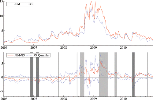
To illustrate the need for a conditional approach, we plot the MES of J.P. Morgan (JPM) and Goldman Sachs (GS), along with their difference and its 5% confidence bounds in Figure 1. Significant differences are marked by shaded regions, dark indicating GS is more risky than JPM and light shading indicating the reverse. This figure illustrates that the MES of the two firms are highly correlated. Until 2008 the point estimates for GS are generally higher than those for JPM, and this order is reversed after 2008. However, although the point estimates may be different, they are not frequently significantly different. GS is more risky on 8.5% of sample days, while JPM’s risk exceeds GS’ on just 5.9% of days, so that the parameters can only be estimated precisely enough on about 14.4% of the days to truly distinguish the two banks. Importantly, significant rejections are clustered with an autocorrelation of 0.7, meaning that the single days where one firm is more risky than the other, are rare.

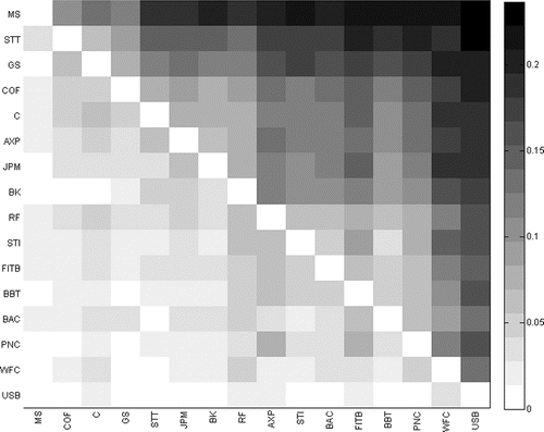
The results for all other pairs are summarized in Figure 2. This figure plots the rejection frequencies for each pair, where the color corresponds to a value determining the frequency at which the firm on the y-axis is found to be more risky than the one on the x-axis. The heatmap shows that even the firms with highest MES are only significantly more risky (at 5%) than firms with the lowest MES in about 20%–25% of the time. On average, across pairs, we find a significant difference between firms on 16.4% of the days. Different significance levels do not change the relative picture much, but at 10% the highest rejection frequencies approach 50%.

6.2 Buckets

In this section, we apply the bucketing procedure to the 94 financial institutions for three systemic risk measures, the MES, the %SRISK, and the ΔCoVaR, which were defined in Examples 2, 3, and 4, respectively. By applying the bucketing procedure, we test whether an absolute ranking can be distinguished. If no absolute ranking can be distinguished, we want to test whether we can, at least, identify buckets of firms that are indistinguishable from each other within the bucket, but distinguishable from firms belonging to lower ranked buckets. The three systemic risk measures are affected differently by the estimation risk, and are also likely to differ in the ordering of their point estimates (Benoit, Colletaz, and Hurlin 2014). As a consequence, different risk measures can lead to different rankings.

Table 3 Bucket allocation top 10

MES				%SRISK				ΔCoVaR
Tick	FWE	FDR	Est.	Tick	FWE	FDR	Est.	Tick	FWE	FDR	Est.
30-06-2008
LEH	1	1	10.287	C	1	1	0.152	FITB	1	1	3.480
MBI	1	1	9.781	BAC	2	2	0.091	HBAN	1	1	2.874
CIT	1	1	8.111	JPM	2	3	0.081	LEH	1	1	2.685
WM	1	1	7.459	MER	2	3	0.078	KEY	1	1	2.372
PFG	1	1	6.563	MS	3	4	0.073	RF	1	1	2.330
ABK	1	2	7.806	FRE	4	5	0.065	C	1	1	2.277
FITB	1	2	7.733	FNM	4	6	0.063	STI	1	1	2.034
C	1	2	5.816	AIG	4	7	0.057	BBT	1	1	2.017
FRE	1	2	5.713	GS	5	7	0.056	AIG	1	1	2.008
MER	2	2	6.248	LEH	6	8	0.052	MI	1	1	1.951
30-01-2009
STT	1	1	22.188	JPM	1	1	0.153	AFL	1	1	9.049
C	1	1	20.884	C	2	2	0.142	PNC	1	1	8.266
HBAN	1	1	20.775	BAC	3	3	0.129	STT	1	1	6.891
FITB	1	1	19.821	WFC	4	4	0.093	FITB	1	1	6.414
PNC	1	1	19.817	AIG	5	5	0.063	BAC	1	1	5.974
AFL	1	1	19.499	GS	5	6	0.061	ACAS	1	1	5.537
LNC	1	1	19.032	MS	6	7	0.046	ALL	1	1	5.487
BAC	1	1	18.491	MET	6	8	0.036	WFC	1	1	5.399
HIG	1	1	17.415	PRU	7	9	0.034	STI	1	1	5.258
PFG	1	1	17.097	HIG	8	10	0.022	C	1	1	5.139

NOTE: This table provides the ranking estimated by the FWE and FDR controlling methods, based on the MES, %SRISK, and ΔCoVaR risk measures. We show only the top 10 of firms sorted by assigned bucket.

Table 4 Number of estimated buckets

		Significance level
		FWE controlling procedure						FDR controlling procedure
Date	#Firms	30%	20%	10%	5%	1%		30%	20%	10%	5%	1%
		MES
30-03-2007	83	5	5	4	4	3		7	7	6	4	3
29-06-2007	83	5	5	3	3	3		7	5	4	4	3
31-12-2007	81	5	5	4	4	3		13	10	8	5	5
29-02-2008	82	6	5	5	4	4		15	12	8	5	4
30-06-2008	82	6	5	5	5	5		11	11	7	6	5
29-08-2008	81	8	8	7	6	5		21	16	10	8	7
30-01-2009	73	6	6	5	4	4		20	15	9	7	5
30-06-2010	75	5	4	3	3	3		9	7	5	5	4
		%SRISK
30-03-2007	14	6	6	6	5	4		7	7	6	6	5
29-06-2007	13	6	6	5	4	4		11	10	7	6	4
31-12-2007	36	17	17	13	11	11		22	21	17	15	12
29-02-2008	37	17	16	15	13	12		26	25	19	17	14
30-06-2008	39	20	18	17	15	12		37	37	26	21	17
29-08-2008	36	16	15	14	13	10		34	33	25	18	15
30-01-2009	53	33	31	29	29	29		49	49	45	39	31
30-06-2010	37	19	18	16	15	11		31	31	22	20	15
		ΔCoVaR
30-03-2007	83	2	2	2	2	1		1	1	1	1	1
29-06-2007	83	1	1	1	1	1		1	1	1	1	1
31-12-2007	81	2	2	1	1	1		2	2	2	2	2
29-02-2008	82	2	2	2	2	1		2	2	2	2	2
30-06-2008	82	3	3	1	2	2		3	3	2	2	2
29-08-2008	81	2	1	2	2	2		2	2	2	2	2
30-01-2009	73	2	2	2	2	2		4	4	4	3	3
30-06-2010	75	1	1	1	1	1		2	2	2	2	2

NOTE: This table reports the sensitivity of the procedures to the level of FWE and FDR that is controlled. We show the total number of firm and the number of buckets they are assigned to.

We estimate the bucket allocation for the MES, %SRISK, and ΔCoVaR on eight predetermined dates coinciding with those considered in Brownlees and Engle (2012). A firm is included in the ranking at a certain date, if the firm still exists and if there are at least 1000 observations up until that date. Table 3 displays the results of the bucketing procedure, with α = 0.05, for 2 days. The results for the remaining days are deferred to, Appendix B. The firms are first ranked in terms of their bucket, and within buckets we order the firms in descending value of their risk measure estimate, even though there is no statistical evidence that their risk is statistically different. We then report the 10 highest ranked firms, as is done in Brownlees and Engle (2012). For each firm, we report the point estimate, as well as the allocated bucket according to the FWE and the FDR method.

The results suggest that it is indeed difficult to find significant differences between the estimated risk measures. Although point estimates may vary considerably, they are not necessarily statistically different. In general, and in line with theory, we find that the FDR rejects more frequently, and we obtain smaller buckets compared to the FWE. In June 2008, the precision of the MES estimates allows for a division of the top 10 risky firms into two buckets. The size of the most risky bucket using FDR is five firms, compared to nine for the FWE.

The point estimates in our ranking are not monotonically decreasing. For instance, in June 2008, based on the FDR method, we find that ABK is in a lower bucket than PFG, despite a higher point estimate. This is a direct consequence of the one-directional approach, and is a feature shared with the MCS (see Hansen, Lunde, and Nason 2011, Table V, where a model with lower average loss is excluded from the MCS). Although PFG has a lower point estimate, its estimation uncertainty is far greater. As such, the procedure cannot reject that its risk is smaller than that of for instance LEH, whereas we can reject that same hypothesis for ABK. Hence, firms with large estimation uncertainty are prudently allocated to high-risk buckets.

The procedure rejects more frequently for the %SRISK, finding a total of six or eight buckets for the top 10 firms. The reason for this is that the liabilities and the market value of the firm, introduced in the definition of the SRISK (see Example 3), add variability between the different point estimates without adding additional estimation risk. In fact, in January 2009 we find an absolute ranking using the FDR method, where each firm has statistically different risk.

Similar to the MES, in our sample it is difficult to statistically distinguish firms based on ΔCoVaR. The ΔCoVaR is defined as the product of a conditional VaR and a quantile regression parameter (see Example 4). Most of the estimation risk comes from the quantile regression. For instance, the highest point forecast of ΔCoVaR is 9.05 for AFL, but its bootstrap standard deviation is close to 4. In an unreported simulation, we find that even if the true DGP is exactly the one assumed here, the standard deviation of the ΔCoVaR is still on average over 40% of its value. These results are in line with those obtained in another context by Guntay and Kupiec (2015). Replacing the quantile estimate γ_α of Example 4 with an ordinary least-square (OLS) estimate significantly reduces the uncertainty, leading to buckets of sizes in between those of MES and %SRISK.

In Table 4, we investigate the sensitivity of the bucketing procedure to the significance level chosen. We report the total number of estimated buckets on each of the 8 days, at five different significance levels. The Model Confidence Set (Hansen, Lunde, and Nason 2011), on which our procedure is based, is commonly estimated using confidence levels upward of 20%. We consider 30%, 20%, 10%, 5%, and 1%, for both FWE and FDR. As a reference, the second column of Table 4 gives the total number of firms under consideration, providing a cap on the number of buckets possible.

As rejection occurs more frequently with higher significance levels, the number of buckets is increasing with the significance level. The FDR procedure detects more buckets than the FWE for each significance level and each risk measure. For instance, for the MES, the FDR procedure estimates up to twice as many buckets than the FWE. With the %SRISK, the FDR procedure using high confidence levels comes close to absolute rankings, with the total number of buckets only slightly lower than the number of firms. Even at very stringent levels, we get interesting rankings with buckets that do not contain more than three or four firms. Finally, significance levels of 30% still do not help with disentangling the ΔCoVaR of different firms on these dates. This reaffirms the uncertainty in the quantile regression estimates.

7. CONCLUSION

This article introduces a bootstrap-based comparison test of two risk measures, as well as an iterative procedure to produce a grouped ranking of N > 2 assets or firms, given their conditional risk measures. These tests can be applied to a wide variety of conditional risk measures, while taking into account their estimation risk. Simulation results on VaR and MES forecasts suggest that the pairwise comparison test has good properties in finite samples, both in terms of size and power. Since the bucketing procedure is clearly a multiple testing problem, we propose two versions, one controlling the FWE rate, and one controlling the FDR rate. Simulations show that both set-ups do control their respective rates, and illustrate the trade-off of using either method depending on the size of the problem.

In the empirical application, we apply the pairwise comparison test to the MES estimates of 16 U.S. G- and D-SIBs. This application points out the advantages of the comparison of conditional risk measures. We highlight the importance of conditional testing, as we observe great time-variation in conditional MES estimates, and from 1 week to the next, firms’ relative ranking often changes. We find that, on most days, due to estimation uncertainty in MES, we cannot distinguish firms in terms of their riskiness. On average across all pairs, we can statistically distinguish firms on 16.4% of days.

We applied the bucketing procedure for three popular systemic risk measures, namely, the MES, the ΔCoVaR, and the SRISK. In our sample, we find that for both versions of the procedure, the MES and ΔCoVaR are estimated with too much uncertainty to reject equality often. For most of the eight dates considered in the application, the first 30 firms belong to the same bucket of riskiest firms. Consequently, ranking firms on the basis of point forecasts of MES and ΔCoVaR may be problematic. However, when applied on %SRISK, our bucketing procedure is able to identify a meaningful ranking of buckets containing equally risky firms in each bucket. This result is mainly due to the differences observed in the liabilities and the market value of the financial institutions over the period 2000–2012. Since the liabilities and market values are not estimated, these differences add cross-sectional variability in the systemic risk measures, without adding additional estimation risk. Our results clearly illustrate the importance of taking into account the estimation risk when establishing a ranking of the financial institutions according to their systemic risk.

SUPPLEMENTARY MATERIALS

The online supplementary materials contains Appendix A (Company tickers) and Appendix B (Bucket allocation top 10).

ACKNOWLEDGMENTS

The authors thank participants at Cluster Risque Financiers, the 7th International MIFN workshop, CREATES seminar, the AFFI 2014, the SoFiE “Systemic Risk and Financial Regulation” Conference, the 8th International Conference on Computational and Financial Econometrics, 2014 Triangle Econometrics Conference, and the 2015 Toulouse Financial Econometrics Conference. The authors thank the editor and two anonymous referees for useful comments. Furthermore, the authors thank Sylvain Benoit, Eric Beutner, Andrew Patton, Christophe Pérignon, and Olivier Scaillet for fruitful discussions. This research was financially supported by the Netherlands Organisation for Scientific Research (NWO) Grants 407-11-042 and 451-12-006. Financial support from the Chair ACPR/Risk Foundation: Regulation and Systemic Risk is gratefully acknowledged. This work was granted access to the HPC resources of Aix-Marseille Université financed by the project Equip@Meso (ANR-10-EQPX-29-01) of the program Investissements d'Avenir supervised by the Agence Nationale de la Recherche.

REFERENCES

- Acharya, V., Engle, R., and Richardson, M. (2012), “Capital Shortfall: A New Approach to Ranking and Regulating Systemic Risks,” The American Economic Review, 102, 59–64.
- Acharya, V., Pedersen, L., Philippon, T., and Richardson, M. (2010), “Measuring Systemic Risk,” New York University Working Paper.
- Adrian, T., and Brunnermeier, M.K. (2014), “CoVaR,” NBER Working Paper No. 17454.
- Bajgrowicz, P., and Scaillet, O. (2012), “Trading Revisited: Persistence Tests, Transaction Costs, and False Discoveries,” Journal of Financial Economics, 106, 473–491.
- Basel Committee on Banking Supervision, (2013), Global Systemically Important Banks: Updated Assessment Methodology and the Higher Loss Absorbency Requirement, Basel: Bank for International Settlements.
- Benjamini, Y., and Hochberg, Y. (1995), “Controlling the False Discovery Rate: A Practical and Powerful Approach to Multiple Testing,” Journal of the Royal Statistical Society, Series B, 57, 289–300.
- Benoit, S., Colletaz, G., and Hurlin, C. (2014), “A Theoretical and Empirical Comparison of Systemic Risk Measures,” University of Orléans Working Paper.
- Brownlees, C., and Engle, R. (2012), “Volatility, Correlation and Tails for Systemic Risk Measurement,” New York University Working Paper.
- Castro, C., and Ferrari, S. (2014), “Measuring and Testing for the Systemically Important Financial Institutions,” Journal of Empirical Finance, 25, 1–14.
- Chan, N., Deng, S., Peng, L., and Xia, Z. (2007), “Interval Estimation of Value-at-Risk Based on GARCH Models With Heavy-Tailed Innovations,” Journal of Econometrics, 137, 556–576.
- Christoffersen, P., and Gonçalves, S. (2005), “Estimation Risk in Financial Risk Management,” Journal of Risk, 7, 1–28.
- Danielsson, J., James, K.R., Valenzuela, M., and Zer, I. (2011), “Model Risk of Systemic Risk Models,” London School of Economics Working Paper.
- Diebold, F., and Mariano, R. (1995), “Comparing Predictive Accuracy,” Journal of Business and Economic Statistics, 13, 253–263.
- Doornik, J. (2012), Object-Oriented Matrix Programming Using Ox (3rd ed.), London: Timberlake Consultants Press and Oxford.
- Engle, R. (2012), “Dynamic Conditional Beta,” New York University Working Paper.
- Escanciano, J., and Olmo, J. (2010), “Backtesting Parametric Value-at-Risk With Estimation Risk,” Journal of Business and Economic Statistics, 28, 36–51.
- ——— (2011), “Robust Backtesting Tests for Value-at-Risk,” Journal of Financial Econometrics, 9, 132–161.
- Francq, C., and Zakoïan, J. (2015), “Risk-Parameter Estimation in Volatility Models,” Journal of Econometrics, 184, 158–173.
- Gouriéroux, C., and Zakoïan, J.-M. (2013), “Estimation Adjusted VaR,” Econometric Theory, 29, 735–770.
- Guntay, L., and Kupiec, P. (2015), “Testing for Systemic Risk Using Stock Returns,” AEI Economic Working Paper 2015-02.
- Hansen, P.R., and Lunde, A. (2006), “Consistent Ranking of Volatility Models,” Journal of Econometrics, 131, 97–121.
- Hansen, P.R., Lunde, A., and Nason, J. (2011), “The Model Confidence Set,” Econometrica, 79, 453–497.
- Hartz, C., Mittnik, S., and Paolella, M. (2006), “Accurate Value-at-Risk Forecasting Based on the Normal-GARCH Model,” Computational Statistics & Data Analysis, 51, 2295–2312.
- Hidalgo, J., and Zaffaroni, P. (2007), “A Goodness-of-Fit Test for ARCH(∞) Models,” Journal of Econometrics, 141, 835–875.
- Laurent, S. (2013), G@RCH 7.0: Estimating and Forecasting ARCH Models, London: Timberlake Consultants Ltd.
- Pascual, L., Romo, J., and Ruiz, E. (2006), “Bootstrap Prediction for Returns and Volatilities in GARCH Models,” Computational Statistics & Data Analysis, 50, 2293–2312.
- Patton, A.J. (2011), “Volatility Forecast Comparison Using Imperfect Volatility Proxies,” Journal of Econometrics, 160, 246–256.
- Reeves, J.J. (2005), “Bootstrap Prediction Intervals for ARCH Models,” International Journal of Forecasting, 21, 237–248.
- Robio, P.O. (1999), “Forecast Intervals in ARCH Models: Bootstrap Versus Parametric Methods,” Applied Economics Letters, 6, 323–327.
- Romano, J.P., Shaikh, A.M., and Wolf, M. (2008a), “Control of the False Discovery Rate Under Dependence Using the Bootstrap and Subsampling,” Test, 17, 417–442.
- ——— (2008b), “Formalized Data Snooping Based on Generalized Error Rates,” Econometric Theory, 24, 404–447.
- Romano, J.P., and Wolf, M. (2005), “Stepwise Multiple Testing as Formalized Data Snooping,” Econometrica, 73, 1237–1282.
- Scaillet, O. (2004), “Nonparametric Estimation and Sensitivity Analysis of Expected Shortfall,” Mathematical Finance, 14, 115–129.
- ——— (2005), “Nonparametric Estimation of Conditional Expected Shortfall,” Insurance and Risk Management Journal, 74, 382–406.
- Shimizu, K. (2013), “The Bootstrap Does not Always Work for Heteroscedastic Models,” Statistics & Risk Modeling, 30, 189–204.
- West, K.D. (1996), “Asymptotic Inference About Predictive Ability,” Econometrica, 64, 1067–1084.
- ——— (2006), “Forecast Evaluation,” in Handbook of Economic Forecasting, eds. G. Elliott, C. Granger, and A. Timmermann, Amsterdam: North Holland Press , pp. 100–134.
- White, H. (2000), “A Reality Check for Data Snooping,” Econometrica, 68, 1097–1126.