Testing the Multivariate Regular Variation Model

Abstract

In this article, we propose a test for the multivariate regular variation (MRV) model. The test is based on testing whether the extreme value indices of the radial component conditional on the angular component falling in different subsets are the same. Combining the test on the constancy across extreme value indices in different directions with testing the regular variation of the radial component, we obtain the test for testing MRV. Simulation studies demonstrate the good performance of the proposed tests. We apply this test to examine two datasets used in previous studies that are assumed to follow the MRV model.

KEYWORDS:

• Extreme value statistics
• Hill estimator
• Local empirical process

1 Introduction

We construct a goodness-of-fit test for the multivariate regular variation (MRV) model. This model has been applied in various areas without a rigorous validation. We aim to provide an easy to implement test, yet applicable to higher dimensional data. Next, we first introduce the notion and relevance of MRV and then explain the heuristics of our approach.

1.1 Multivariate Regular Variation

Large price fluctuations in finance and large losses in insurance exhibit power-like tails (see, e.g., Gabaix 2009). The univariate regular varying distributions are often used to capture such heavy tailed phenomena. The MRV model generalizes this to the higher dimensional situation to allow the marginal distributions to be regularly varying with a flexible tail dependence structure. Typical examples of MRV include elliptical distributions with a regularly varying radial component, multivariate Student’s t distributions, multivariate α-stable distributions, Archimedean copulas with regularly varying generator and marginals (Weng and Zhang 2012), among others.

The MRV model is related to multivariate extreme value theory. Consider independent and identically distributed (iid) random vectors from an MRV model. Then the component-wise maxima of these random vectors, with the same normalization for each marginal, weakly converge to a multivariate extreme value distribution (see, e.g., Resnick 2013 for details).

The MRV model possesses a few convenient theoretical properties which promote its vast applications in different areas. For example, stationary solutions to stochastic recurrence equations have regularly varying marginals and follow the MRV model (see, e.g., Kesten 1973). As a consequence, widely used models in finance for assets returns, such as the ARCH and GARCH models, have finite-dimensional distributions following the MRV model (see, e.g., Davis and Mikosch 1998; Stărică 1999; Basrak, Davis, and Mikosch 2002a, 2002b). In addition, as a semiparametric model, the MRV model assumes only a limit relation in the tail region of a multivariate distribution. Consequently it allows for a flexible dependence structure across several heavy-tailed random variables (see, e.g., Lindskog 2004; Resnick 2007 for more details). Due to these modeling features, in risk management, MRV is often assumed to be the model for multiple underlying risk factors. The tail behavior of the aggregated risk based on multiple risk factors satisfying the MRV model can be explicitly derived (see, e.g., Hauksson et al. 2001; Barbe, Fougeres, and Genest 2006; Embrechts, Lambrigger, and Wüthrich 2009). Furthermore, portfolio diversification under the MRV model was investigated in Mainik and Rüschendorf (2010), Zhou (2010), and Mainik and Embrechts (2013), among others. Besides the applications in finance and insurance, the MRV model is also applied in telecommunications networks (see, e.g., Resnick and Samorodnitsky 2015; Samorodnitsky et al. 2016). Here it is important to verify the MRV model for real data by means of a hypothesis test. Validation of the MRV model justifies the derivations and conclusions of these studies.

The relevance of the MRV model is among others that the multivariate outlying regions are homothetic when taking different degrees of outlyingness. This makes extrapolation from intermediately extreme events to very extreme events possible, which makes MRV a powerful model (see, e.g., He and Einmahl 2017). Characterizing extreme outlyingness is not only important to detect outliers or anomalies, but it is also reveals the joint extreme behavior of multivariate risks, which in turn can be relevant for defining stress testing scenarios. Clearly a check on the MRV model is needed to make this often required extrapolation possible.

In most of the applications, the MRV model is assumed without a formal validation. This might be due to the fact that there is no formal goodness-of-fit test of the MRV model in the literature. The only exception is Einmahl and Krajina (2020), which provides a formal test for the MRV model but the test is restricted to the bivariate case. The approach in there is very different: it uses empirical likelihood and does not use extreme value index estimation. In fact, testing whether a higher dimensional dataset follows a MRV model by starting from its very definition introduced in Section 2 is challenging. This is because one needs to deal with the dimensionality, and the complex dependence structures among the dimensions. In this article, inspired by an important feature of MRV model, we construct a formal goodness-of-fit test for the MRV model. The heuristics of the method are explained in the next section. Our proposed test can be applied in any dimension.

We demonstrate the finite sample performance of the proposed tests through various models that either satisfy the null hypothesis or fall in the alternative. Especially, simulations based on three-dimensional MRV models are also performed to illustrate how our testing procedure works in higher dimension. We also apply the test to two real datasets: exchange rates (Yen-Dollar, Pound-Dollar), and stock indices (S&P, FTSE, Nikkei). Our study shows that these two datasets follow the MRV model, which implies that the MRV model is indeed a realistic assumption in these applications to financial markets. Besides, it provides support for the empirical studies in Cai, Einmahl, and De Haan (2011) and He and Einmahl (2017), in which the MRV model is assumed without a formal test.

1.2 Heuristics of Our Method

The existing studies employing the MRV model at best apply a simple, informal, check for the validity of the MRV model. The simple check is on the equality of all the extreme value indices of the left and right tails of all marginal distributions implied by the MRV model. Some other application studies conduct a more careful test by comparing extreme value indices beyond the marginals, albeit still informal (see, e.g., Cai, Einmahl, and De Haan 2011).

Inspired by the informal comparison of extreme value indices, the rationale behind our formal test is as follows. By using polar coordinates, random variables following a MRV model can be mapped into a univariate radial component and a multivariate angular component. The radius follows a univariate regular variation model with a positive extreme value index and is asymptotically independent of the angular component. The independence in the limit guarantees that the extreme value index of the radius conditional on the angular component is the same regardless where the conditioning angular component lies. The informal test relying on marginals can be viewed as testing the constancy of extreme value indices in the directions lining up with the axes in the original coordinate system. We compare the extreme value indices along other directions beyond the axes. The proposed test formalizes such a comparison into a goodness-of-fit test for the MRV model. More specifically, our proposed test combines testing the constancy of the extreme value indices of the radii conditional on various directions of the angular component with testing the regular variation of the radius. Tests for the latter problem are known but here the challenge is to combine them with our new test on the extreme value indices and turn it into one correct formal test. This will be achieved by proving asymptotic independence of the two test statistics.

Testing the constancy of extreme value indices in all “directions” of the angular component is somewhat similar to the constant extreme value index test in Einmahl, de Haan, and Zhou (2016); see T₃ and T₄ therein. In the null hypothesis therein, the observations are generated from different univariate distributions with the same extreme value index but different “scale.” In other words, the extreme value indices are the same at all locations, while the scale varies according to a fixed covariate indicating the location. Our test can be viewed as testing the constancy of the extreme value indices across random covariates, that is, the angular component induces the scale. More specifically, we employ a test that is similar to the T₄ test in Einmahl, de Haan, and Zhou (2016), but with random covariates. The present approach is, however, substantially different.

The study of estimating the extreme value index with a random covariate received attention only recently in both parametric and nonparametric setups. Much of the work focused on the case that the conditional distribution of the response variable belongs to the class of Pareto-type distributions, such as Wang and Tsai (2009), Daouia et al. (2011), Gardes and Girard (2012), Wang, Li, and He (2012), Wang and Li (2013), Gardes and Stupfler (2014), Goegebeur, Guillou, and Schorgen (2014), and Goegebeur, Guillou, and Stupfler (2015). A few follow-up works generalize to the complete max-domain of attractions of the extreme value distribution; see Daouia, Gardes, and Girard (2013), Stupfler (2013), and Goegebeur, Guillou, and Osmann (2014). In the current article, we do not impose a parametric model between the extreme value index and the covariates. Neither do we emphasize on the estimation of the conditional extreme value index. Instead, we focus on testing the constancy of the directional extreme value indices.

In the proposed tests, besides the usual tuning parameter threshold k, the “number of directions” is used as an extra tuning parameter. A good choice of that parameter depends on both the number of observations and the underlying probability distribution. This introduces a level of subjectivity. In applications, it is recommended to apply the test with a few values for both tuning parameters.

The rest of the article is organized as follows. Section 2 provides the main theoretical results: the constancy test of the directional extreme value indices and how to combine it with testing the regular variation of the radius. The simulation study and application can be found in Sections 3 and 4, respectively. Section 5 concludes the article. The proofs are deferred to Appendix A.

2 Methodology

We define MRV via a transformation to polar coordinates. For an arbitrary norm $\Vert ·\Vert$, the polar coordinate transform of a vector x is defined as(1) $$\mathcal{P}(\mathbf{x})=\left(\Vert \mathbf{x}\Vert ,{\Vert \mathbf{x}\Vert }^{-1}\mathbf{x}\right),$$(1) where $\Vert \mathbf{x}\Vert$ is called the radial component and ${\Vert \mathbf{x}\Vert }^{-1}\mathbf{x}$ is called the angular component of x. A random vector X with polar transformation $\mathcal{P}(\mathbf{X})$ is said to be multivariate regularly varying, if there exists a probability measure $\Psi$ on the Borel σ-algebra $\mathcal{B}({\mathcal{S}}^{d-1})$, where ${\mathcal{S}}^{d-1}=\left\{\mathbf{s}\in {\mathbb{R}}^d:\Vert \mathbf{s}\Vert =1\right\}$, and $\gamma >0$, such that, for all x > 0, as $t\to \infty$,(2) $$\frac{\mathrm{Pr}\left(\Vert \mathbf{X}\Vert >tx,{\Vert \mathbf{X}\Vert }^{-1}\mathbf{X}\in ·\right)}{\mathrm{Pr}\left(\Vert \mathbf{X}\Vert >t\right)}\stackrel{\mathrm{v}}{\to }{x}^{-1/\gamma }\Psi (·),\hspace{1em}\text{on}\mathcal{B}\left({\mathcal{S}}^{d-1}\right),$$(2) where $\stackrel{\mathrm{v}}{\to }$ denotes vague convergence; $\Psi$ is called the spectral measure.

With a random sample of observations drawn from the distribution of X, we intend to test whether the underlying distribution satisfies the MRV model defined by (2). It is straightforward to derive from (2) that for any Borel set $B\in \mathcal{B}({\mathcal{S}}^{d-1})$, if $\Psi (B)>0$, then$$\underset{t\to \infty }{\lim }\frac{\mathrm{Pr}\left(\Vert \mathbf{X}\Vert >tx|{\Vert \mathbf{X}\Vert }^{-1}\mathbf{X}\in B\right)}{\mathrm{Pr}\left(\Vert \mathbf{X}\Vert >t|{\Vert \mathbf{X}\Vert }^{-1}\mathbf{X}\in B\right)}=x^{-1/\gamma },$$which implies that $\Vert \mathbf{X}\Vert$ is regularly varying in any “direction” defined by B. Therefore, we shall estimate the extreme value index $\gamma =\gamma (B)$ using the observations of $\Vert \mathbf{X}\Vert$ conditioning on ${\Vert \mathbf{X}\Vert }^{-1}\mathbf{X}\in B$ and further test whether $\gamma (B)$ is constant across various (disjoint) sets B with $\Psi (B)>0$. Besides, we need to test whether the radius $\Vert \mathbf{X}\Vert$ possesses a regularly varying tail.

The rest of Section 2 is organized in the following way. First, in Section 2.1, we establish a test in the two-dimensional setup for the null hypothesis of having a constant $\gamma (B)$. Second, testing the univariate regular variation of $\Vert \mathbf{X}\Vert$ is well established in the literature. The difficulty here is to avoid a multiple testing problem, that is, we need to be able to combine the two tests into one. We shall establish this in Section 2.2. Although these two subsections focus on the bivariate case, our testing procedure can be extended to the higher dimensional case. Section 2.3 explains the test for higher dimensional MRV.

2.1 Testing the Bivariate MRV Model

For a bivariate random vector ${(X,Y)}^T$, consider the following polar transformation(3) $$\{\begin{array}{c}X=R\hspace{0.17em}\text{cos}\hspace{0.17em}\Theta ,\hfill \\ Y=R\hspace{0.17em}\text{sin}\hspace{0.17em}\Theta .\hfill \end{array}$$(3)

Then ${(X,Y)}^T$ is one-to-one mapped to ${(R,\Theta )}^T$ with $R\ge 0$ and $\Theta \in [0,2\pi ]$. With abuse of notation, we regard $\Psi$ as the distribution function of the spectral measure on $[0,2\pi ]$. For convenience we assume that F_R, the distribution function of R, is continuous. Write $U_R=1/{(1-F_R)}^{\leftarrow }$, where “←” denotes the left-continuous inverse function.

Let ${(X_1,Y_1)}^T,\dots ,{(X_n,Y_n)}^T$ be iid observations from the distribution of ${(X,Y)}^T$. By the polar transformation (3), we obtain the transformed pairs ${(R_1,{\Theta }_1)}^T,\dots ,{(R_n,{\Theta }_n)}^T$, which is the starting point for constructing the test. We first define the estimator of the extreme value index γ in a subregion. Order $R_1,\dots ,R_n$ as $R_{1,n}\le \cdots \le R_{n,n}$ and take $R_{n-k,n}$ ($k\in \{1,\dots ,n-1\}$) as the common threshold.

For any $\delta >0$ and $0\le {\theta }_1<{\theta }_2\le 2\pi$ satisfying $\Psi ({\theta }_2)-\Psi ({\theta }_1)>\delta$, we define a Hill estimator $\widehat{\gamma }({\theta }_1,{\theta }_2)$ as the estimator using the observations corresponding to ${\theta }_1<{\Theta }_i\le {\theta }_2$ as follows$$\widehat{\gamma }({\theta }_1,{\theta }_2)=\frac{\sum _{i=1}^n(\hspace{0.17em}\text{log}\hspace{0.17em}{R}_i-\hspace{0.17em}\text{log}\hspace{0.17em}{R}_{n-k,n})1_{\left\{R_i>R_{n-k,n},{\theta }_1<{\Theta }_i\le {\theta }_2\right\}}}{\sum _{i=1}^n{1}_{\left\{R_i>R_{n-k,n},{\theta }_1<{\Theta }_i\le {\theta }_2\right\}}}.$$

Observe that $\Psi ({\theta }_2)-\Psi ({\theta }_1)>\delta$ guarantees ${\sum }_{i=1}^n{1}_{\left\{{\theta }_1<{\Theta }_i\le {\theta }_2\right\}}\stackrel{P}{\to }\infty$, as $n\to \infty$. Denote the distribution function of the spectral measure also with $\Psi$. A natural estimator for $\Psi$ (see Einmahl, de Haan, and Huang 1993) is given by$$\widehat{\Psi }(\theta )=\frac{1}{k}\sum _{i=1}^n{1}_{\left\{R_i>R_{n-k,n},{\Theta }_i\le \theta \right\}}.$$

To test the constancy of $\gamma (B)$, we estimate $\gamma (B)$ from various subsamples and compare these estimators. More specifically, first for a fixed integer m, we split the data with largest k radii into m disjoint parts with about equal number of observations. The cutoff points are defined as follows. Denote ${\theta }_j={\Psi }^{\leftarrow }(j/m)$ and ${\widehat{\theta }}_j={\widehat{\Psi }}^{\leftarrow }(j/m)$ for $j=0,1,\dots ,m$. Clearly ${\theta }_0={\widehat{\theta }}_0=0$ and ${\theta }_m={\widehat{\theta }}_m=2\pi$. Define ${\widehat{\gamma }}_j:=\widehat{\gamma }({\widehat{\theta }}_{j-1},{\widehat{\theta }}_j)$ and ${\widehat{\gamma }}_{\text{all}}:=\widehat{\gamma }(0,2\pi )$. In Figure 1, we provide a visualization of the choice of the cutoff points.

Fig. 1 The illustration of the choice of cutoff points in constructing the test statistic T_n with four blocks. The red line represents the threshold above which there are 20 points. The blue vertical lines are the cutoff points such that in each block there are 5 points above the red line.

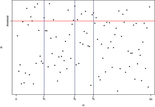
Next, we define the test statistic as$$T_n:=\frac{k}{m}\sum _{j=1}^m{\left(\frac{{\widehat{\gamma }}_j}{{\widehat{\gamma }}_{\text{all}}}-1\right)}^2.$$

Clearly, it compares all the ${\widehat{\gamma }}_j$ obtained in the m subregions to ${\widehat{\gamma }}_{\text{all}}$ which uses all peaks over threshold.

To establish the asymptotic theory of the test statistic T_n, we assume a second-order condition as follows.

Assumption 2.1.

There exists a function β such that $\beta (t)\to 0$ as $t\to \infty$ and for any $x_0>0$, as $t\to \infty$,$$\underset{x>x_0,0\le \theta \le 2\pi }{\sup }\left|x^{1/\gamma }\frac{\mathrm{Pr}(R>tx,\Theta \le \theta )}{\mathrm{Pr}(R>t)}-\Psi (\theta )\right|=O(\beta (t)).$$

Further assume that $\Psi$ is continuous on $[0,2\pi ]$.

Assumption 2.1 requires uniform convergence in the MRV definition in (2) with some convergence rate β. It is a natural and rather weak second-order condition imposed on R and Θ jointly. Such a second-order condition is standard in the literature of extreme value statistics (see, e.g., Einmahl, de Haan, and Huang 1993; De Haan and Ferreira 2006, Condition 7.3.4). In contrast, in the often used one-dimensional second-order condition pointwise convergence is considered, which yields a set of uniform inequalities (see, e.g., Beirlant et al. 2004; De Haan and Ferreira 2006). Our condition does not require the existence of a density; see condition (a) in Cai, Einmahl, and De Haan (2011) where the density is already needed in the definition of the extreme risk regions studied in there. For more details about multivariate regular variation of densities, see De Haan and Resnick (1987). Naturally, when constructing examples of distributions that satisfy Assumption 2.1 we often consider distributions that do have densities. A large class of examples is given by spherical or elliptical distributions, with the radius R satisfying an appropriate univariate second-order condition such as taking $\theta =2\pi$ in Assumption 2.1. Examples in this class are the bivariate (or multivariate) Student’s t distributions.

Now we are ready to present the asymptotic behavior of T_n under the null hypothesis; the proof of this theorem is deferred to Appendix A.1.

Theorem 1.

If Assumption 2.1 holds and the sequence k satisfies $k\to \infty ,k/n\to 0$ and $\sqrt{k}\beta (U_R(n/k))\to 0$ as $n\to \infty$, then for a fixed integer $m\ge 2$, we have that as $n\to \infty$,$$T_n\stackrel{d}{\to }{\chi }_{m-1}^2.$$

Intuitively, the theorem follows from the fact that all ${\widehat{\gamma }}_j$ are asymptotically normal with iid asymptotic limits, while ${\widehat{\gamma }}_{\text{all}}$ is the sample mean of ${\widehat{\gamma }}_j$. Consequently, T_n, as the scaled sample variance of all ${\widehat{\gamma }}_j$, is asymptotically chi-squared distributed. The theoretical conditions on k, which are standard in extreme value statistics, are to ensure that the ${\widehat{\gamma }}_j$‘s and ${\widehat{\gamma }}_{\text{all}}$ are asymptotically unbiased. These conditions are crucial for deriving the chi-squared limit.

2.2 Dealing With the Radial Component

Besides testing for the same extreme value index in every direction, we also need to test whether the radial component R possesses a regularly varying tail. We use the PE test in Hüsler and Li (2006, (1.3)). The test statistic is defined as(4) $$Q_n=k{\int }_0^1{\left(\frac{\hspace{0.17em}\text{log}\hspace{0.17em}{R}_{n-\left[kt\right],n}-\hspace{0.17em}\text{log}\hspace{0.17em}{R}_{n-k,n}}{{\widehat{\gamma }}_{\text{all}}}+\hspace{0.17em}\text{log}\hspace{0.17em}t\right)}^2{t}^{\eta }dt.$$(4)

Under the null hypothesis that R possesses a regularly varying tail and a restriction on k, $Q_n\stackrel{d}{\to }Q$ as $n\to \infty$, with(5) $$Q={\int }_0^1{\left(t^{-1}B(t)+\hspace{0.17em}\text{log}\hspace{0.17em}t{\int }_0^1{s}^{-1}B(s)ds\right)}^2{t}^{\eta }dt,$$(5) where B is a standard Brownian bridge. According to Hüsler and Li (2006), $\eta =0.5$ is a good choice.

To avoid a multiple testing problem, we need to investigate the joint asymptotic behavior of our test statistic T_n in Theorem 1 and Q_n. The following theorem shows that the two are asymptotically independent. The proof is again deferred to Appendix A.2.

Theorem 2.

Under the conditions of Theorem 1, we have that$$(T_n,Q_n)\stackrel{d}{\to }(T,Q),\hspace{1em}n\to \infty ,$$where $T\sim {\chi }_{m-1}^2$ and Q is as in (5), and T and Q are independent.

Following Theorem 2, we can construct a combined test based on T_n and Q_n. For a significance level $\alpha \in (0,1)$, this combined test rejects if the test based on T_n or that on Q_n rejects for significance level $1-\sqrt{1-\alpha }$. The combined test has a p-value$$1-{\left(1-\min (p_1,p_2)\right)}^2,$$where p₁ and p₂ are the p-values of the T_n and Q_n tests, respectively.

2.3 Dealing With Higher Dimensions

In Sections 2.1 and 2.2, we constructed tests for the bivariate MRV model. The same method can be applied in higher dimensions. In this section, we discuss the general idea and some practical suggestions for higher dimensional cases.

Suppose $\mathbf{X}={(X_1,X_2,\dots ,X_d)}^T$ is a d-dimensional random vector. With the polar transformation (1), we can decompose X into a radial component $\Vert \mathbf{X}\Vert$ and an angular component ${\Vert \mathbf{X}\Vert }^{-1}\mathbf{X}\in {\mathcal{S}}^{d-1}$. Testing whether X follows a MRV model boils down to testing whether $\Vert \mathbf{X}\Vert$ possesses a regularly varying tail and whether the extreme value indices are the same in any “direction” specified by a Borel set $B\in \mathcal{B}({\mathcal{S}}^{d-1})$. For the former testing problem, we refer to the test in Section 2.2. Here we only focus on the latter.

To construct a test for the constancy of the extreme value index, we need to divide the unit sphere ${\mathcal{S}}^{d-1}$ into m subregions containing about equal number of exceedances. One can achieve this by processing the division dimension by dimension. We illustrate the idea for Dimension 3.

Let ${(X,Y,Z)}^T$ be a three-dimensional random vector. Consider the usual polar coordinates transformation$$\{\begin{array}{c}X=R\hspace{0.17em}\text{cos}\hspace{0.17em}\Omega \hspace{0.17em}\text{cos}\hspace{0.17em}\Theta ,\hfill \\ Y=R\hspace{0.17em}\text{cos}\hspace{0.17em}\Omega \hspace{0.17em}\text{sin}\hspace{0.17em}\Theta ,\hfill \\ Z=R\hspace{0.17em}\text{sin}\hspace{0.17em}\Omega .\hfill \end{array}$$

Clearly, its inverse transformation maps any ${(X,Y,Z)}^T$ to ${(R,\Theta ,\Omega )}^T$ with $R\ge 0,\Theta \in [0,2\pi ]$ and $\Omega \in [-\pi /2,\pi /2]$. Suppose we observe an iid sample drawn from the distribution of ${(X,Y,Z)}^T$. We transform each observation ${(X_i,Y_i,Z_i)}^T$ into the polar coordinates ${(R_i,{\Theta }_i,{\Omega }_i)}^T$ for $i=1,2,\dots ,n$. Again order $R_1,\dots ,R_n$ as $R_{1,n}\le \cdots \le R_{n,n}$.

Let $m=m_1{m}_2$ with m₁, m₂ positive integers. We intend to find cutoff points ${\widehat{\theta }}_j$ and ${\widehat{\omega }}_{j,l},j=0,1,\dots ,m_1$ and $l=0,1,\dots ,m_2$, to split the observations into m blocks such that there are about k/m exceedances falling into each block of the form $\left\{{\widehat{\theta }}_{j-1}<{\Theta }_i\le {\widehat{\theta }}_j,{\widehat{\omega }}_{j,l-1}<{\Omega }_i\le {\widehat{\omega }}_{j,l}\right\}$, for any $j=1,2,\dots ,m_1$ and $l=1,2,\dots ,m_2$.

Consider the distribution function $\Psi$ of the spectral measure for $\theta \in [0,2\pi ]$ and $\omega \in [-\pi /2,\pi /2]$. A natural estimator for $\Psi$ is$$\widehat{\Psi }(\theta ,\omega )=\frac{1}{k}\sum _{i=1}^n{1}_{\left\{R_i>R_{n-k,n},{\Theta }_i\le \theta ,{\Omega }_i\le \omega \right\}}.$$

Write ${\widehat{\Psi }}_{\Theta }(\theta )=\widehat{\Psi }(\theta ,\pi /2)$. In the first step, we define the cutoff points ${\widehat{\theta }}_j={\widehat{\Psi }}_{\Theta }^{\leftarrow }(j/m_1)$, for $j=1,2,\dots ,m_1$. In the second step, for each given $j=1,2,\dots ,m_1$, denote$${\widehat{\Psi }}_{\Omega ,j}(\omega )=\widehat{\Psi }({\widehat{\theta }}_j,\omega )-\widehat{\Psi }({\widehat{\theta }}_{j-1},\omega ).$$

Then, the cutoff points are ${\widehat{\omega }}_{j,l}={\widehat{\Psi }}_{\Omega ,j}^{\leftarrow }(l/m_2)$, for $l=1,2,\dots ,m_2$. Lastly, we can construct the extreme value index estimator in each subregion as$${\widehat{\gamma }}_{j,l}=\frac{\sum _{i=1}^n(\hspace{0.17em}\text{log}\hspace{0.17em}{R}_i-\hspace{0.17em}\text{log}\hspace{0.17em}{R}_{n-k,n})1_{\left\{R_i>R_{n-k,n},{\widehat{\theta }}_{j-1}<{\Theta }_i\le {\widehat{\theta }}_j,{\widehat{\omega }}_{j,l-1}<{\Omega }_i\le {\widehat{\omega }}_{j,l}\right\}}}{\sum _{i=1}^n{1}_{\left\{R_i>R_{n-k,n},{\widehat{\theta }}_{j-1}<{\Theta }_i\le {\widehat{\theta }}_j,{\widehat{\omega }}_{j,l-1}<{\Omega }_i\le {\widehat{\omega }}_{j,l}\right\}}},$$for all $j=1,2,\dots ,m_1$ and $l=1,2,\dots ,m_2$. Similarly, we denote the Hill estimator of the radii with ${\widehat{\gamma }}_{\text{all}}=\frac{1}{k}{\sum }_{i=1}^n(\hspace{0.17em}\text{log}\hspace{0.17em}{R}_i-\hspace{0.17em}\text{log}\hspace{0.17em}{R}_{n-k,n})1_{\left\{R_i>R_{n-k,n}\right\}}.$ The test statistic T_n in the three-dimensional case is given by$$T_n:=\frac{k}{m}\sum _{j=1}^{m_1}\sum _{l=1}^{m_2}{\left(\frac{{\widehat{\gamma }}_{j,l}}{{\widehat{\gamma }}_{\text{all}}}-1\right)}^2.$$

To establish the asymptotic behavior of T_n, we need a corresponding second-order condition in the three-dimensional case as follows.

Assumption 2.2.

There exists a function $\beta (t)$ such that $\beta (t)\to 0$ as $t\to \infty$ and for any $x_0>0$, as $t\to \infty$,$$\underset{x>x_0,0\le \theta \le 2\pi ,-\pi /2\le \omega \le \pi /2}{\sup }|x^{1/\gamma }\frac{\mathrm{Pr}(R>tx,\Theta \le \theta ,\Omega \le \omega )}{\mathrm{Pr}(R>t)}$$$$-\Psi (\theta ,\omega )|=O(\beta (t)).$$

Further assume that $\Psi$ is continuous on $[0,2\pi ]\times [-\pi /2,\pi /2]$.

Theorem 3.

If Assumption 2.2 holds and the sequence k satisfies $k\to \infty ,k/n\to 0$ and $\sqrt{k}\beta (U_R(n/k))\to 0$ as $n\to \infty$, then for a fixed positive integer $m\ge 2$, we have that as $n\to \infty$,$$T_n\stackrel{d}{\to }{\chi }_{m-1}^2.$$

Moreover the statement of Theorem 2 remains true in Dimension 3.

Since the proof of this theorem is very much the same as that of Theorems 1 and 2, we confine ourselves to only stating and proving the main tool in the proof of Theorem 3, Proposition 1, in arbitrary Dimension d. This proposition then also shows that dimensions higher than 3 can be treated in a similar way.

We shall consider the three-dimensional case in the simulation study in detail; see Section 3.

3 Simulation

In this section, we demonstrate the finite sample performance of our proposed tests for MRV. We simulate l = 1000 samples with sample size n = 5000. For each sample, we perform the tests for each (asymptotic) significance level $\alpha =1\%,5\%,$ and 10%. We report the number of samples for which we reject the null.

3.1 Simulations Under the Null Hypothesis, Dimension 2

We first consider two bivariate distributions under the null hypothesis.

Distribution 1. Let ${(X,Y)}^T$ follow a centered Student’s t distribution with ν degrees of freedom and 2 × 2 scale matrix with 1 as diagonal elements and $s\in (-1,1)$ as off-diagonal elements. Then ${(X,Y)}^T$ follows a MRV distribution with extreme value index $1/\nu$ and the corresponding spectral measure has a positive density. We vary the degrees of freedom ($\nu =0.5,2$) and take $s=0.3,0.7$ to examine the impact of these parameters.

Distribution 2. Consider the polar coordinates ${(R,\Theta )}^T$ of ${(X,Y)}^T$ following the transformation in (3). Assume U and V are two independent uniform-(0,1) random variables. Let $\Theta =2\pi V$, and$$R=\{\begin{array}{ccc}{F}_1^{\leftarrow }(1-U),\hfill & \hfill & V\le 1/2,\hfill \\ F_2^{\leftarrow }(1-U),\hfill & \hfill & 1/2<V\le 1,\hfill \end{array}$$with $F_i(x)=1-{(\frac{1}{x+1})}^{{\beta }_i}$ for x > 0 and i = 1, 2. If ${\beta }_1\cancel{=}{\beta }_2$, then ${(X,Y)}^T$ follows a MRV distribution that has a spectral measure with zero density on half of the unit circle. In this distribution R and Θ are dependent, but asymptotically independent. We consider different combinations of the extreme value indices (${\beta }_1=0.5,{\beta }_2=2$ and ${\beta }_1=1,{\beta }_2=3$).

Since the Q_n test has been well studied in the literature, for the null distributions we only study the T_n test. We choose m = 4 and m = 6 in Tables 1 and 2, respectively.

The T_n test performs well for all 6 distributions under the null hypothesis. In particular, it performs better when m = 4 than when m = 6 under the current sample size of 5000. When m = 6, the test performs slightly better for k = 500. For m = 6 and k = 250, the number of exceedances in each block is too low to make the asymptotic theory work well. In general, the test performs well under the null hypothesis if there is fast convergence in (2) and in Assumption 2.1. In that case the chi-squared distribution is a good approximation to the distribution of T_n and hence the size of the test is close to the targeted significance level.

Table 1 The total number of rejections under the null (m = 4).

Distribution		k = 250			k = 500
	α	10%	5%	1%	10%	5%	1%
D1	s = 0.7, $\nu =0.5$	95	52	7	98	44	8
	s = 0.7, ν = 2	86	47	15	109	54	10
	s = 0.3, $\nu =0.5$	106	55	10	101	50	13
	s = 0.3, ν = 2	93	46	9	126	65	16
D2	${\beta }_1=0.5,{\beta }_2=2$	100	49	14	102	46	8
	${\beta }_1=1,{\beta }_2=3$	104	54	4	139	71	18

Table 2 The total number of rejections under the null (m = 6).

Distribution		k = 250			k = 500
	α	10%	5%	1%	10%	5%	1%
D1	s = 0.7, $\nu =0.5$	80	46	13	73	32	5
	s = 0.7, ν = 2	85	41	6	109	49	10
	s = 0.3, $\nu =0.5$	70	35	7	95	48	9
	s = 0.3, ν = 2	64	36	11	108	48	16
D2	${\beta }_1=0.5,{\beta }_2=2$	78	36	6	85	39	9
	${\beta }_1=1,{\beta }_2=3$	75	40	7	143	74	18

3.2 Simulations Under The Alternative; Dimension 2

We consider two bivariate distributions under the alternative. We choose m = 4 below because of the better behavior than m = 6 under the null. Besides the T_n test, we also check the performance of the combined test for the alternative distributions. Recall that to achieve a significance level of $\alpha =1\%,5\%,$ or 10%, we should reject the combined null if either of the T_n or Q_n test rejects at the level $1-\sqrt{1-\alpha }\approx 0.5\%,2.5\%,$ or 5.1%, respectively.

Distribution 3. Consider the polar coordinates ${(R,\Theta )}^T$ of ${(X,Y)}^T$ following the transformation in (3). Let U and V be iid uniform-(0,1) and set $R=U^{-1/\beta }$, which implies that R is regularly varying with extreme value index $1/\beta$. Define$$\Theta =\{\begin{array}{ccc}\pi V,\hfill & \hfill & \frac{1}{2^n}<U\le \frac{1}{2^{n-1}}\mathrm{}\text{with}\mathrm{}\text{an}\mathrm{}\text{odd}\mathrm{}\text{integer}\mathrm{}n,\hfill \\ \pi +\pi V,\hfill & \hfill & \frac{1}{2^n}<U\le \frac{1}{2^{n-1}}\mathrm{}\text{with}\mathrm{}\text{an}\mathrm{}\text{even}\mathrm{}\text{integer}\mathrm{}n.\hfill \end{array}$$

Then the distribution of ${(X,Y)}^T$ is not MRV. In this distribution, R and Θ are not asymptotically independent, which results in a nontrivial counter-example. We choose $\beta =0.5,1$.

Distribution 4. Let Z₁ and Z₂ be iid Pareto with extreme value index $1/\beta$. We consider two cases.

Distribution 4.1. Let ${(X,Y)}^T={(Z_1,2Z_2)}^T$. Then ${(X,Y)}^T$ possesses a spectral measure with unequal masses $1/(1+2^{\beta })$ and $2^{\beta }/(1+2^{\beta })$ at 0 and $\pi /2$, respectively.

Distribution 4.2. Let ${(X,Y)}^T={(Z_1,Z_2)}^T$. Then ${(X,Y)}^T$ possesses a spectral measure with mass 1/2 at 0 and at $\pi /2$.

For both Distributions 4.1 and 4.2, the spectral measure is not continuous, which falls in the alternative. These two distributions are degenerated MRV, which falls outside our null hypothesis. Again we take $\beta =0.5,2$.

The simulation results for Distributions 3 and 4 are shown in Table 3. For data simulated from these alternative distributions, the powers of both T_n and the combined test are high, except when using a lower k and α for Distribution 3.

Table 3 The total number of rejections under the alternative.

Distribution			k = 250			k = 500
		α	10%	5%	1%	10%	5%	1%
D3	$\beta =0.5$	Tn	728	631	403	950	900	793
		Combined	657	535	346	911	861	739
	β = 1	T n	741	631	425	955	923	785
		Combined	656	555	344	929	881	722
D4.1	$\beta =0.5$	Tn	1000	1000	1000	1000	1000	1000
		Combined	1000	1000	1000	1000	1000	1000
	β = 2	Tn	977	955	860	1000	1000	1000
		Combined	960	929	781	1000	1000	999
D4.2	$\beta =0.5$	Tn	1000	1000	1000	1000	1000	1000
		Combined	1000	1000	1000	1000	1000	1000
	β = 2	Tn	988	973	886	1000	1000	999
		Combined	977	943	841	1000	1000	999

3.3 Dimension 3

In Dimension 3 we consider the following two distributions, one falls in the null hypothesis, whereas the other one falls in the alternative. Again we take $m=4(m_1=m_2=2)$.

Distribution 5. Let ${(X,Y,Z)}^T$ follow a centered Student’s t distribution with ν degrees of freedom and scale matrix$$\Sigma =\left(\begin{array}{ccc}1& s& 0\\ s& 1& s\\ 0& s& 1\end{array}\right),$$with $s\in (-1,1)$. Similar to Distribution 1, this distribution is MRV with extreme value index $1/\nu$ and the corresponding spectral measure has a positive density. We choose $\nu =0.5,1$ and $s=0.3,0.7$.

Distribution 6. Let X, Y, and Z be three independent random variables following Pareto distributions with extreme value indices $1/{\beta }_1,1/{\beta }_2$, and $1/{\beta }_3$, respectively. In this case the distribution function of the spectral measure is not continuous, which falls in the alternative.

The simulation results for Distributions 5 and 6 are shown in Table 4. Again, the numbers of rejections match the significance levels under the null (Distribution 5) since there is fast enough convergence in Assumption 2.2. Under Distribution 6 the power can be seen to be higher for the heavier-tailed distributions: when the marginal extreme value index is higher, the observations corresponding to high radius are more concentrated on the axes, which yields more different estimators (in the blocks) of the extreme value index.

Table 4 The total number of rejections in Dimension 3.

Distribution			k = 250			k = 500
		α	10%	5%	1%	10%	5%	1%
D5	s = 0.7, $\nu =0.5$	Tn	99	59	11	98	54	14
	s = 0.7, ν = 1	Tn	102	48	11	101	51	12
	s = 0.3, $\nu =0.5$	Tn	99	50	8	104	53	8
	s = 0.3, ν = 1	Tn	102	54	11	99	52	14
D6	${\beta }_1={\beta }_2={\beta }_3=0.5$	Tn	673	564	319	914	858	676
		Combined	586	467	285	867	791	620
	${\beta }_1={\beta }_2={\beta }_3=1$	Tn	594	481	233	809	722	529
		Combined	526	417	226	872	797	608
	${\beta }_1={\beta }_2={\beta }_3=2$	Tn	448	334	138	708	581	337
		Combined	392	300	176	641	545	354

4 Application

In this section, we test two datasets that are claimed to be MRV in Cai, Einmahl, and De Haan (2011) and He and Einmahl (2017), respectively.

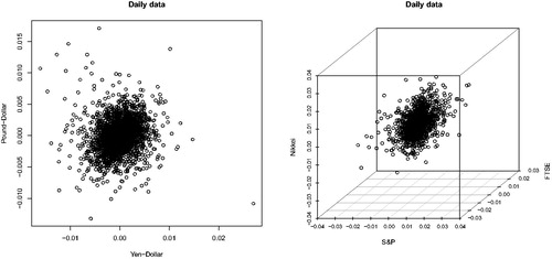
The first dataset we consider is the one used in Cai, Einmahl, and De Haan (2011): daily exchange rates of Yen-Dollar and Pound-Dollar from January 4, 1999 to July 31, 2009. Cai, Einmahl, and De Haan (2011) considered daily log returns, that is,$$X_i=\hspace{0.17em}\text{log}\hspace{0.17em}\left(\frac{P_{i+1}}{P_i}\right),$$where P_i is the exchange rate on day i. We obtain the data, which consist of 2758 observations, from Thomson Reuters. The left panel of Figure 2 presents the scatterplot of the pair (Yen-Dollar, Pound-Dollar).

Fig. 2 Scatterplots for (Yen-Dollar, Pound-Dollar) and (S&P, FTSE, Nikkei).

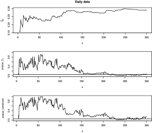
We show the Hill estimates of the extreme value index of the radius R by varying k, the p-values of our T_n test by varying k, and the p-values of the combined test (combining T_n and Q_n tests) by varying k. We take 4 blocks (m = 4) in conducting the T_n test and the combined test.

According to Cai, Einmahl, and De Haan (2011), the estimated extreme value index for R is ${\widehat{\gamma }}_R=0.256$, which corresponds to a threshold k around 70–80 in the upper graph of Figure 3. At this level of k, from both T_n and combined tests we do not reject the null at a significance level of 5%, see the middle and lower graphs in Figure 3. In general, we do not reject that (Yen-Dollar, Pound-Dollar) follows an MRV distribution for a wide range of relevant k less than 200. In other words, the MRV model is validated and we can proceed with statistical inference based on the MRV model. In particular, this supports the extrapolation technique for obtaining the extreme risk regions in Cai, Einmahl, and De Haan (2011), which yield an alarm system for risk management.

Fig. 3 The pair (Yen-Dollar, Pound-Dollar). The upper graph shows the Hill estimates for the radius R. The middle graph shows the p-values of the T_n test. The lower graph shows the p-values of the combined test.

The second dataset is from He and Einmahl (2017) and consists of daily international market price indices of the Standard and Poors (S&P) 500 index from the USA, the Financial Times Stock Exchange FTSE 100 index from the UK and the Nikkei 225 index from Japan. The sample period is from July 2nd, 2001, to June 29th, 2007. Again, daily log returns are constructed. We obtain the dataset, which has in total 1564 observations, from the accompanying file of that article.

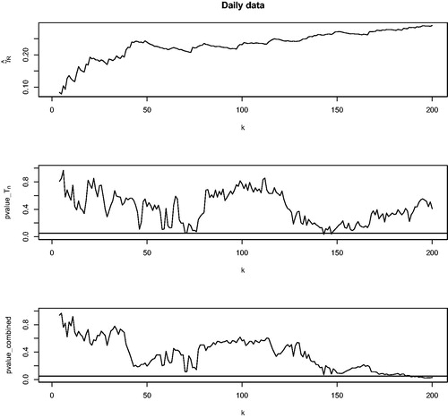
We consider the triplet (S&P, FTSE, Nikkei) and test whether it follows an MRV distribution using our tests. The right panel of Figure 2 presents the scatterplot of the triplet. Again, our tests are carried out by plotting the p-values against various levels of k. Our analysis for the triplet is shown in Figure 4. In He and Einmahl (2017), when estimating the left and right extreme value indices of the three series, the threshold k is chosen at 80. At k = 80, we do not reject the null that the triplet follows an MRV distribution at the 5% level by both tests. In general, we do not reject for k less than 150. Thus, the MRV model is validated. This justifies the approach in He and Einmahl (2017) for obtaining extreme depth-based quantile regions which measure the practically relevant outlyingness, as discussed in Section 1.

Fig. 4 The triplet (S&P, FTSE, Nikkei). The upper graph shows the Hill estimates for the radius R. The middle graph shows the p-values of the T_n test. The lower graph shows the p-values of the combined test.

One potential drawback of our analysis is that we regard the observations as independent without accounting for the potential serial dependence. When the data possess weak serial dependence, for example, satisfying β-mixing conditions, the test might be still valid subject to some adjustment. More specifically, we conjecture that the statistic $T_n/{\sigma }^2$ converges to the same ${\chi }_{m-1}^2$-distribution limit, where ${\sigma }^2$ is an adjusting factor determined by the serial dependence. Here for “positive” serial dependence, that is, when extremes are likely to occur on consecutive days, we have ${\sigma }^2>1$ (see, e.g., Drees 2000), in which the asymptotic normality of the Hill estimator was studied under the β-mixing conditions. Intuitively, dependent data contain less information than the same amount of independent data, which leads to an increase of estimation error. In that case, the current test can be regarded as a conservative test: if we do not reject the null for the data using the current test, we will not reject the null after adjusting for serial dependence. Given that for both datasets we consider, we do not reject the null by regarding the data as independent, we conjecture that a proper test accounting for serial dependence will not reject the null either. Had we observed a result rejecting the null, we would have to account for the impact of serial dependence.

Another way to handle serial dependence without estimating ${\sigma }^2$ is to consider the observations on even (or odd) days only and carry out the tests by regarding those observations as independent. The almost independence among every other day data is supported by various empirical studies on the extremal index for the financial data. They show that the average cluster size of extremes is around 2 and some even close to 1 (see, e.g., McNeil 1998; Poon, Rockinger, and Tawn 2003; Hamidieh, Stoev, and Michailidis 2009). We have performed such an analysis and obtained the same conclusion.

5 Conclusion

In this article, we construct a goodness-of-fit test for the MRV model. The test is based on comparing the extreme value indices of the radial component conditional on the angular component falling in different, disjoint subsets. This results in the T_n test. In addition, we test whether the radius follows a univariate regular variation model by the Q_n test. The two tests can be easily combined thanks to their asymptotic independence. The proposed tests can be extended to higher dimensional cases. Simulation studies for both two-dimensional and three-dimensional cases show that the T_n test performs well and has good power properties, especially for the heavier tailed distributions. The combined test is applied to a few datasets in the literature that are assumed to be MRV. Our test supports making the MRV assumptions for these datasets.

As in any test in extreme value analysis, one needs to choose the tuning parameters. Besides the usual parameter k, here one also needs to choose the number of blocks m. The higher m, the more directions are being compared. In practice, one has to choose a low m to ensure sufficient observations in each block. A good choice of m depends on both the number of observations n and the underlying probability distribution. In applications, it is recommended to choose a few values for both tuning parameters k and m.

Acknowledgments

We thank an associate editor and three referees for their thoughtful comments which greatly helped improving the article.

Appendix A:

Proofs

A.1 Proof of Theorem 1

We begin with establishing the main tool used in the proof of Theorem 1, the asymptotic behavior of an appropriate local empirical process. We provide this main tool in arbitrary Dimension d. In this way it is useful for proving Theorems 1 and 3 and their higher dimensional generalizations. Without presenting the general transformation to polar coordinates explicitly, note that the now (d – 1)-variate $\mathit{\theta }$ runs through $T_d:=[\underset{\_}{\mathit{\theta }},\overline{\mathit{\theta }}]$, where $\underset{\_}{\mathit{\theta }}={(0,-\pi /2,-\pi /2,\dots ,-\pi /2)}^T$ and $\overline{\mathit{\theta }}={(2\pi ,\pi /2,\pi /2,\dots ,\pi /2)}^T$ are two vectors in ${\mathbb{R}}^{d-1}$. The local empirical process that we consider is, in the obvious notation,$$\begin{array}{c}{\mathbb{S}}_n(x,\mathit{\theta }):=\sqrt{k}(\frac{1}{k}\sum _{i=1}^n{1}_{\left\{R_i>U_R\left(\frac{n}{k}x\right),{\mathbf{\Theta }}_i\le \mathit{\theta }\right\}}\\ \mathrm{\hspace{1em}}\mathrm{\hspace{1em}}-\frac{n}{k}\mathrm{Pr}\left(R_1>U_R\left(\frac{n}{k}x\right),{\mathbf{\Theta }}_1\le \mathit{\theta }\right)),\end{array}$$for $x\ge x_1(>0),\mathit{\theta }\in T_d.$ We need the generalization of Assumption 2.1.

Assumption A.1.

There exists a function β such that $\beta (t)\to 0$ as $t\to \infty$ and for any $x_0>0$, as $t\to \infty$,$$\underset{x>x_0,\mathit{\theta }\in T_d}{\sup }\left|x^{1/\gamma }\frac{\mathrm{Pr}(R_1>tx,{\mathbf{\Theta }}_1\le \mathit{\theta })}{\mathrm{Pr}(R_1>t)}-\Psi (\mathit{\theta })\right|=O(\beta (t)).$$

Proposition 1.

If Assumption A.1 holds and the sequence k satisfies $k\to \infty ,k/n\to 0$ and $\sqrt{k}\beta (U_R(n/k))\to 0$ as $n\to \infty$, then, there exists a sequence of d-variate Wiener processes W_n, defined on the probability space accommodating $(R_1,{\mathbf{\Theta }}_1),\dots ,(R_n,{\mathbf{\Theta }}_n)$, with$$\text{Cov}(W_n(x_1,{\mathit{\theta }}_1),W_n(x_2,{\mathit{\theta }}_2))=\left(x_1\wedge x_2\right)\Psi ({\mathit{\theta }}_1\wedge {\mathit{\theta }}_2),$$such that for any given $x_1>0$ and $0<\zeta \le 1/2$, as $n\to \infty$,(A.1) $$\underset{x\ge x_1,\mathit{\theta }\in T_d}{\sup }{x}^{1/2-\zeta }\left|{\mathbb{S}}_n(x,\mathit{\theta })-W_n(1/x,\mathit{\theta })\right|\stackrel{P}{\to }0.$$(A.1)

Proof of Proposition 1.

We start by proving (A.1) without the weight function $x^{1/2-\zeta }$. This is achieved by applying Lemma 3.1 in Einmahl, de Haan, and Sinha (1997). Write $U_i=1-F_R(R_i)$, then $U_1,\dots ,U_n$ are iid uniform-(0,1). Further write $Y_i^{(n)}=\left(\frac{n}{k}{U}_i,{\mathbf{\Theta }}_i\right)$ and consider the sets $A(y,\mathit{\theta })=[0,y]\times [\underset{\_}{\mathit{\theta }},\mathit{\theta }],y\le 1/x_1,\mathit{\theta }\in T_d.$ Then we can rewrite the local empirical process as$${\mathbb{S}}_n\left(x,\mathit{\theta }\right)=\frac{n}{\sqrt{k}}\left(\frac{1}{n}\sum _{i=1}^n{1}_{\left\{Y_i^{(n)}\in A(1/x,\mathit{\theta })\right\}}-\mathrm{Pr}\left(Y_1^{(n)}\in A(1/x,\mathit{\theta })\right)\right).$$

In order to apply Lemma 3.1 in Einmahl, de Haan, and Sinha (1997), we only need to check that as $n\to \infty$,(A.2) $$\underset{y\le 1/x_1,\mathit{\theta }\in T_d}{\sup }\left|\frac{n}{k}\mathrm{Pr}(Y_1^{(n)}\in A(y,\mathit{\theta }))-\mu (A(y,\mathit{\theta }))\right|\to 0,$$(A.2) for some finite measure μ.

By taking $\mathit{\theta }=\overline{\mathit{\theta }}$ in Assumption A.1, we obtain that as $t\to \infty$,$$\underset{x>x_0}{\sup }\left|\frac{\mathrm{Pr}(R_1>tx)}{\mathrm{Pr}(R_1>t)}-x^{-1/\gamma }\right|=O(\beta (t)),$$which implies a second order result for the U_R function:(A.3) $$\underset{x\ge x_1}{\sup }\left|\frac{U_R(tx)}{U_R(t)}-x^{\gamma }\right|=O(\beta (U_R(t))),$$(A.3) where x₁ is any positive constant such that $x_1>x_0^{1/\gamma }$. Replacing t and tx by $U_R(n/k)$ and $U_R(n/(ky))$, respectively, in Assumption A.1, and by (A.3), we obtain that as $n\to \infty$,$$\hspace{1em}\underset{y\le 1/x_1,\mathit{\theta }\in T_d}{\sup }\left|\frac{n}{k}\mathrm{Pr}(U_1<ky/n,{\mathbf{\Theta }}_1\le \mathit{\theta })-y\Psi (\mathit{\theta })\right|$$$$=O(\beta (U_R(n/k)))\to 0,$$ which verifies (A.2) with $\mu (A(y,\mathit{\theta }))=y\Psi (\mathit{\theta })$. Consequently, we obtain that as $n\to \infty$, for any $x_1>0$,(A.4) $$\underset{x\ge x_1,\mathit{\theta }\in T_d}{\sup }\left|{\mathbb{S}}_n(x,\mathit{\theta })-W_n(1/x,\mathit{\theta })\right|\stackrel{P}{\to }0,$$(A.4) where W_n is a sequence of d-variate Wiener processes as in Proposition 1. (To return to the original probability space of the $(R_i,{\mathbf{\Theta }}_i)$, see Einmahl 1997,p. 52.)

Next, we introduce the weight function and write $y=1/x$. Given (A.4), for a proof of (A.1) it suffices to prove that for any given $\epsilon >0$ and $0<\zeta <1/2$, there exists $\eta =\eta (\epsilon ,\zeta )>0$ such that for sufficiently large n,(A.5) $$\mathrm{Pr}\left(\underset{y\le \eta ,\mathit{\theta }\in T_d}{\sup }{y}^{-1/2+\zeta }\left|{\mathbb{S}}_n(1/y,\mathit{\theta })\right|>\epsilon \right)<3\epsilon ,$$(A.5) (A.6) $$\mathrm{Pr}\left(\underset{y\le \eta ,\mathit{\theta }\in T_d}{\sup }{y}^{-1/2+\zeta }\left|W_n(y,\mathit{\theta })\right|>\epsilon \right)<\epsilon .$$(A.6)

The inequality in (A.6) is well-known (see, e.g., Orey and Pruitt 1973, Theorem 2.2). To prove (A.5), we split the interval $(0,\eta ]$ into three parts $I_1:=(0,\tau /k],I_2:=(\tau /k,1/k^a]$ and $I_3:=(1/k^a,\eta ]$, with $a={(1+2\zeta )}^{-1}$ and $\tau >0$. We prove that for all i = 1, 2, 3, for large n,$$\mathrm{Pr}\left(\underset{y\in I_i,\mathit{\theta }\in T_d}{\sup }{y}^{-1/2+\zeta }\left|{\mathbb{S}}_n(1/y,\mathit{\theta })\right|>\epsilon \right)<\epsilon .$$

First, we deal with $y\in I_1$. Observe that if ${\min }_{1\le i\le n}{U}_i>\tau /n$, then for $y\le \tau /k$ we have $\left|{\mathbb{S}}_n(1/y,\mathit{\theta })\right|\le \sqrt{k}y.$ Therefore, by choosing τ small enough$$\begin{array}{c}\mathrm{Pr}\left(\underset{y\in I_1,\mathit{\theta }\in T_d}{\sup }{y}^{-1/2+\zeta }\left|{\mathbb{S}}_n(1/y,\mathit{\theta })\right|>\epsilon \right)\\ \le \mathrm{Pr}\left(\underset{y\in I_1}{\sup }\sqrt{k}{y}^{1/2+\zeta }>\epsilon ,\underset{1\le i\le n}{\min }{U}_i>\tau /n\right)+\mathrm{Pr}\left(\underset{1\le i\le n}{\min }{U}_i\le \tau /n\right)\\ =\mathrm{Pr}\left(\underset{1\le i\le n}{\min }{U}_i\le \tau /n\right)<\epsilon .\end{array}$$

To deal with I₂ and I₃, we need the following lemma. Consider the empirical process$${\alpha }_n(x,\mathit{\theta })=\sqrt{n}\left(\frac{1}{n}\sum _{i=1}^n{1}_{\left\{U_i\le x,{\mathbf{\Theta }}_i\le \mathit{\theta }\right\}}-\mathrm{Pr}(U_1\le x,{\mathbf{\Theta }}_1\le \mathit{\theta })\right).$$

Lemma 4.

For $0<b_1<b_2\le 1/4,0\le \xi \le 1/2$ and $\lambda \ge 0$,

$\hspace{1em}\mathrm{Pr}(\underset{b_1\le x\le b_2,\mathit{\theta }\in T_d}{\sup }{x}^{-1/2+\xi }\left|{\alpha }_n(x,\mathit{\theta })\right|\ge \lambda )\le C{\int }_{b_1/2}^{2b_2}\frac{1}{s}\hspace{0.17em}\text{exp}\hspace{0.17em}(-\frac{{\lambda }^2}{4}\frac{1}{s^{2\xi }}\psi \left(\frac{\lambda }{n^{1/2}{b}_1^{1/2+\xi }}\right))ds,$(A.7)where $C=C(d)>0$ is a constant, and $\psi (\lambda )=2{\lambda }^{-2}[(1+\lambda )\hspace{0.17em}\text{log}\hspace{0.17em}(1+\lambda )-\lambda ]$ is a continuous, decreasing function defined on $[-1,\infty )$.

We will omit the proof of this lemma, but just mention that it follows that of Inequality (2.6) in Einmahl (1987) for Dimension 1 (since x is one-dimensional), but then uses Inequality (2.5) in there for Dimension d.

Next, we deal with $y\in I_2$. Since ${\mathbb{S}}_n(1/y,\mathit{\theta })=\sqrt{\frac{n}{k}}{\alpha }_n\left(\frac{ky}{n},\mathit{\theta }\right)$, by applying Lemma 4 with ξ = 0, we have that for large n $$\begin{array}{c}\mathrm{Pr}\left(\underset{y\in I_2,\mathit{\theta }\in T_d}{\sup }{y}^{-1/2+\zeta }\left|{\mathbb{S}}_n(1/y,\mathit{\theta })\right|>\epsilon \right)\\ =\mathrm{Pr}\left(\underset{\frac{\tau }{n}\le x\le \frac{k^{1-a}}{n},\mathit{\theta }\in T_d}{\sup }{x}^{-1/2+\zeta }\left|{\alpha }_n(x,\mathit{\theta })\right|>\epsilon {\left(\frac{k}{n}\right)}^{\zeta }\right)\\ \le \mathrm{Pr}\left(\underset{\frac{\tau }{n}\le x\le \frac{k^{1-a}}{n},\mathit{\theta }\in T_d}{\sup }{x}^{-1/2}\left|{\alpha }_n(x,\mathit{\theta })\right|>\epsilon k^{\zeta a}\right)\\ \le C{\int }_{\frac{\tau }{2n}}^{\frac{2k^{1-a}}{n}}\frac{1}{s}ds·\hspace{0.17em}\text{exp}\hspace{0.17em}\left(-\frac{1}{4}{\epsilon }^2{k}^{2\zeta a}\psi \left(\frac{\epsilon k^{\zeta a}}{{\tau }^{1/2}}\right)\right)\\ \le C_1(\hspace{0.17em}\text{log}\hspace{0.17em}k)\hspace{0.17em}\text{exp}\hspace{0.17em}\left(-k^{\zeta a}\right)<\epsilon ,\end{array}$$where C₁ is some constant.

Lastly, we deal with $y\in I_3$ by directly applying Lemma 4 with $\xi =\zeta$. We have that$$\begin{array}{c}\mathrm{Pr}\left(\underset{y\in I_3,\mathit{\theta }\in T_d}{\sup }{y}^{-1/2+\zeta }\left|{\mathbb{S}}_n(1/y,\mathit{\theta })\right|>\epsilon \right)\\ =\mathrm{Pr}\left(\underset{\frac{k^{1-a}}{n}\le x\le \frac{k\eta }{n},\mathit{\theta }\in T_d}{\sup }{x}^{-1/2+\zeta }\left|{\alpha }_n(x,\mathit{\theta })\right|>\epsilon {\left(\frac{k}{n}\right)}^{\zeta }\right)\\ \le C{\int }_0^{\frac{2\eta k}{n}}\frac{1}{s}\hspace{0.17em}\text{exp}\hspace{0.17em}\left(-\frac{{\epsilon }^2{k}^{2\zeta }}{4}\frac{1}{s^{2\zeta }{n}^{2\zeta }}\psi \left(\frac{\epsilon k^{\zeta }}{k^{(1/2+\zeta )(1-a)}}\right)\right)ds\\ \stackrel{t=\frac{n}{k}s}{=}C{\int }_0^{2\eta }\frac{1}{t}\hspace{0.17em}\text{exp}\hspace{0.17em}\left(-\frac{{\epsilon }^2}{4t^{2\zeta }}\psi (\epsilon )\right)dt.\end{array}$$

By choosing a sufficiently small $\eta =\eta (\epsilon ,\zeta )$, this bound is less than ε. □

We now return to the setup of Theorem 1, that is, the two-dimensional case. By applying Proposition 1 (with d = 2), we prove the joint asymptotic normality for the estimators of the directional extreme value indices with fixed cutoff points, $\widehat{\gamma }({\theta }_1,{\theta }_2)$.

Theorem 5.

Under the conditions of Theorem 1, with the same sequence of bivariate Wiener processes W_n as in Proposition 1, for any $\delta >0$ and uniformly for all ${\theta }_1,{\theta }_2$ satisfying $0\le {\theta }_1<{\theta }_2\le 2\pi$ and $\Psi ({\theta }_2)-\Psi ({\theta }_1)>\delta$, as $n\to \infty$,$$\begin{array}{c}\sqrt{k}\left(\widehat{\gamma }({\theta }_1,{\theta }_2)-\gamma \right)=\gamma ({\int }_0^1\frac{W_n(x,{\theta }_2)-W_n(x,{\theta }_1)}{\Psi ({\theta }_2)-\Psi ({\theta }_1)}\frac{dx}{x}\\ -\frac{W_n(1,{\theta }_2)-W_n(1,{\theta }_1)}{\Psi ({\theta }_2)-\Psi ({\theta }_1)})+o_P(1).\end{array}$$

Proof of Theorem 5.

We obtain from (A.1) that

$\underset{x\ge x_1}{\sup }{x}^{1/2-\zeta }\left|({\mathbb{S}}_n(x,{\theta }_2)-{\mathbb{S}}_n(x,{\theta }_1))-(W_n(1/x,{\theta }_2)-W_n(1/x,{\theta }_1))\right|\hspace{1em}=o_P(1),$(A.8)where the $o_P(1)$-term should be read as uniformly for all $0\le {\theta }_1<{\theta }_2\le 2\pi$ such that $\Psi ({\theta }_2)-\Psi ({\theta }_1)>\delta$. In the sequel of the proof all $o_P(1)$-terms should be read as uniformly for such θ₁ and θ₂.

Now consider (A.8) with x replaced by $\frac{k}{n}\frac{1}{1-F_R(U_R(n/k)u)}$, with $u\ge u_0$ for any $u_0>0$. Assumption 2.1 implies that as $n\to \infty$,$$u^{1/\gamma }\frac{1-F_R(U_R(n/k)u)}{k/n}=1+O(\beta (U_R(n/k)))\to 1.$$

Hence, we can replace the weight function in this new version of (A.8) by $u^{(1/2-\zeta )/\gamma }$.

For the two ${\mathbb{S}}_n$ terms we have uniformly for all $u\ge u_0$, as $n\to \infty$,(A.9) $$\begin{array}{c}{u}^{(1/2-\zeta )/\gamma }({\mathbb{S}}_n\left(\frac{k}{n}\frac{1}{1-F_R(U_R(n/k)u)},{\theta }_2\right)\\ \hspace{1em}-{\mathbb{S}}_n\left(\frac{k}{n}\frac{1}{1-F_R(U_R(n/k)u)},{\theta }_1\right))\\ =u^{(1/2-\zeta )/\gamma }\sqrt{k}(\frac{1}{k}\sum _{i=1}^n{1}_{\left\{R_i>U_R\left(\frac{n}{k}\right)u,{\theta }_1<{\Theta }_i\le {\theta }_2\right\}}\\ -\frac{n}{k}\mathrm{Pr}\left(R>U_R\left(\frac{n}{k}\right)u,{\theta }_1<\Theta \le {\theta }_2\right))\\ =u^{(1/2-\zeta )/\gamma }\sqrt{k}(\frac{1}{k}\sum _{i=1}^n{1}_{\left\{R_i>U_R\left(\frac{n}{k}\right)u,{\theta }_1<{\Theta }_i\le {\theta }_2\right\}}\\ \mathrm{\hspace{1em}}\mathrm{\hspace{1em}}-u^{-1/\gamma }(\Psi ({\theta }_2)-\Psi ({\theta }_1)))+o(1).\end{array}$$(A.9)

Finally, by the modulus of continuity results for Wiener processes (see Orey and Pruitt 1973, Theorem 2.1) we have that as $n\to \infty$,$$\begin{array}{c}\underset{u\ge u_0,0<\theta \le 2\pi }{\sup }{u}^{(1/2-\zeta )/\gamma }|W_n\left(\frac{n}{k}\left(1-F_R(U_R(n/k)u)\right),\theta \right)\\ -W_n\left(u^{-1/\gamma },\theta \right)|\le u^{(1/2-\zeta )/\gamma }{(u^{-1/\gamma }{o}_P(1))}^{1/2-\zeta }=o_P(1).\end{array}$$

Together with (A.9), we obtain that the new version of (A.8) now reads as(A.10) $$\begin{array}{c}\underset{u\ge u_0}{\sup }{u}^{(1/2-\zeta )/\gamma }|\sqrt{k}(\frac{1}{k}\sum _{i=1}^n{1}_{\left\{R_i>U_R\left(\frac{n}{k}\right)u,{\theta }_1<{\Theta }_i\le {\theta }_2\right\}}-u^{-1/\gamma }(\Psi ({\theta }_2)\\ -\Psi ({\theta }_1)))-\left(W_n\left(u^{-1/\gamma },{\theta }_2\right)-W_n\left(u^{-1/\gamma },{\theta }_1\right)\right)|=o_P(1).\end{array}$$(A.10)

By taking ${\theta }_1=0$ and ${\theta }_2=2\pi$ in (A.10) and using the Vervaat (1972) lemma, we obtain that

$\sqrt{k}(\frac{R_{n-k,n}}{U_R\left(\frac{n}{k}\right)}-1)=\gamma W_n(1,2\pi )+o_P(1).$(A.11)

Notice that the result in (A.10) is parallel to Theorem 5.1.4 in De Haan and Ferreira (2006). Therefore, using (A.10) and (A.11) the proof of the theorem can be completed along similar lines as in the proof of Example 5.1.5 (asymptotic normality of the Hill estimator using the tail empirical process) there. □

Finally, we apply Theorem 5 to handle the estimators of the directional extreme value indices when using estimated cutoff points, that is, the ${\widehat{\gamma }}_j$ in Section 2.1.

Proof of Theorem 1.

By taking $u=\frac{R_{n-k,n}}{U_R\left(\frac{n}{k}\right)}$ and ${\theta }_1=0$ in (A.10), and further applying (A.11), we obtain that as $n\to \infty$,$$\begin{array}{c}\underset{\theta \in [0,2\pi ]}{\sup }\left|\sqrt{k}\left(\widehat{\Psi }(\theta )-\Psi (\theta )\right)-\left(W_n\left(1,\theta \right)-\Psi (\theta )W_n(1,2\pi )\right)\right|\\ \hspace{1em}=o_P(1).\end{array}$$

Using this in conjunction with Theorem 5 we have as $n\to \infty$,$$\begin{array}{c}\sqrt{k}\left({\widehat{\gamma }}_j-\gamma \right)=m\gamma ({\int }_0^1(W_n(x,{\widehat{\theta }}_j)-W_n(x,{\widehat{\theta }}_{j-1}))\frac{dx}{x}-(W_n(1,{\widehat{\theta }}_j)\\ \hspace{1em}-W_n(1,{\widehat{\theta }}_{j-1})))+o_P(1)\\ =m\gamma ({\int }_0^1(W_n(x,{\theta }_j)-W_n(x,{\theta }_{j-1}))\frac{dx}{x}-(W_n(1,{\theta }_j)\\ \hspace{1em}-W_n(1,{\theta }_{j-1})))+o_P(1)\\ =:\sqrt{m}\gamma N_j+o_P(1),\end{array}$$where $N_j\sim N(0,1)$ and the second step is due to the uniform continuity of W_n. Next, by applying Theorem 5 for ${\theta }_1=0$ and ${\theta }_2=2\pi$, we obtain that as $n\to \infty$,$$\sqrt{k}\left({\widehat{\gamma }}_{\text{all}}-\gamma \right)=\sqrt{m}\gamma \overline{N}+o_P(1),$$ with $\overline{N}=\frac{1}{m}{\sum }_{j=1}^m{N}_j$. Hence, we have as $n\to \infty$,$$T_n=\sum _{j=1}^m{\left(N_j-\overline{N}\right)}^2+o_P(1).$$

Using the independent increments property of the Wiener processes W_n we have that $N_1,\dots ,N_m$ are independent, which yields the stated ${\chi }_{m-1}^2$-limit. □

A.2 Proof of Theorem 2

Proof of Theorem 2.

From the proof of Theorem 1, we obtain that the limit of T_n depends on the process W_n defined in Proposition 1. Notice that the limit of the Q_n statistics is related to the asymptotic expansion of the tail quantile process based on $R_1,\dots ,R_n$ (see, e.g., De Haan and Ferreira 2006, Theorem 5.2.12). In our setup, this refers the approximating univariate Wiener process is $W_n(·,2\pi )$. Therefore, with the same steps as in the proof of Theorem 5.2.12 in De Haan and Ferreira (2006), we obtain that as $n\to \infty$,$$\left|Q_n-{\int }_0^1{\left(B_n(t,2\pi )+\hspace{0.17em}\text{log}\hspace{0.17em}t{\int }_0^1{B}_n(s,2\pi )ds\right)}^2{t}^{\eta }dt\right|\stackrel{P}{\to }0,$$where$$B_n\left(s,\theta \right)=s^{-1}{W}_n(s,\theta )-W_n\left(1,\theta \right).$$

To prove the theorem, it suffices to show that the constructing component for the limit of Q_n $$L_n(t)=B_n\left(t,2\pi \right)+\hspace{0.17em}\text{log}\hspace{0.17em}t{\int }_0^1{B}_n(s,2\pi )ds$$is independent of the constructing component of T_n in Theorem 1 $$M_n(\theta )={\int }_0^1{B}_n(u,\theta )du.$$

Since $(L_n,M_n)$ is a Gaussian process, it suffices to show that $\mathrm{E}\left[L_n(t)M_n(\theta )\right]=0,$ for $t\in [0,1],\theta \in [0,2\pi ]$. This easily follows from$$\mathrm{E}\left[B_n\left(s,\theta \right)B_n\left(u,\zeta \right)\right]=\left(\frac{s\wedge u}{su}-1\right)\Psi (\theta \wedge \zeta ).$$

□

Funding

John Einmahl holds the Arie Kapteyn Chair 2019–2022 and gratefully acknowledges the corresponding research support.

References

- Barbe, P., Fougeres, A.-L., and Genest, C. (2006), “On the Tail Behavior of Sums of Dependent Risks,” ASTIN Bulletin: The Journal of the IAA, 36, 361–373. DOI: https://doi.org/10.1017/S0515036100014550.
- Basrak, B., Davis, R. A., and Mikosch, T. (2002a), “A Characterization of Multivariate Regular Variation,” The Annals of Applied Probability, 12, 908–920. DOI: https://doi.org/10.1214/aoap/1031863174.
- Basrak, B., Davis, R. A., and Mikosch, T. (2002b), “Regular Variation of GARCH Processes,” Stochastic Processes and Their Applications, 99, 95–115.
- Beirlant, J., Goegebeur, Y., Segers, J., and Teugels, J. L. (2004), Statistics of Extremes: Theory and Applications, Chichester: Wiley.
- Cai, J. J., Einmahl, J. H. J., and De Haan, L. (2011), “Estimation of Extreme Risk Regions Under Multivariate Regular Variation,” The Annals of Statistics, 39, 1803–1826. DOI: https://doi.org/10.1214/11-AOS891.
- Daouia, A., Gardes, L., and Girard, S. (2013), “On Kernel Smoothing for Extremal Quantile Regression,” Bernoulli, 19, 2557–2589. DOI: https://doi.org/10.3150/12-BEJ466.
- Daouia, A., Gardes, L., Girard, S., and Lekina, A. (2011), “Kernel Estimators of Extreme Level Curves,” Test, 20, 311–333. DOI: https://doi.org/10.1007/s11749-010-0196-0.
- Davis, R. A., and Mikosch, T. (1998), “The Sample Autocorrelations of Heavy-Tailed Processes With Applications to ARCH,” The Annals of Statistics, 26, 2049–2080. DOI: https://doi.org/10.1214/aos/1024691368.
- De Haan, L., and Ferreira, A. (2006), Extreme Value Theory: An Introduction, New York: Springer-Verlag.
- De Haan, L., and Resnick, S. (1987), “On Regular Variation of Probability Densities,” Stochastic Processes and Their Applications, 25, 83–93. DOI: https://doi.org/10.1016/0304-4149(87)90191-8.
- Drees, H. (2000), “Weighted Approximations of Tail Processes for β-Mixing Random Variables,” The Annals of Applied Probability, 10, 1274–1301. DOI: https://doi.org/10.1214/aoap/1019487617.
- Einmahl, J. H. J. (1987), Multivariate Empirical Processes, CWI Tract (Vol. 32), Amsterdam: Stichting Mathematisch Centrum, Centrum voor Wiskunde en Informatica, available at https://ir.cwi.nl/pub/12752.
- Einmahl, J. H. J. (1997), “Poisson and Gaussian Approximation of Weighted Local Empirical Processes,” Stochastic Processes and Their Applications, 70, 31–58.
- Einmahl, J. H. J., de Haan, L., and Huang, X. (1993), “Estimating a Multidimensional Extreme-Value Distribution,” Journal of Multivariate Analysis, 47, 35–47. DOI: https://doi.org/10.1006/jmva.1993.1069.
- Einmahl, J. H. J., de Haan, L., and Sinha, A. K. (1997), “Estimating the Spectral Measure of an Extreme Value Distribution,” Stochastic Processes and Their Applications, 70, 143–171. DOI: https://doi.org/10.1016/S0304-4149(97)00065-3.
- Einmahl, J. H. J., de Haan, L., and Zhou, C. (2016), “Statistics of Heteroscedastic Extremes,” Journal of the Royal Statistical Society, Series B, 78, 31–51. DOI: https://doi.org/10.1111/rssb.12099.
- Einmahl, J. H. J., and Krajina, A. (2020), “Empirical Likelihood Based Testing for Multivariate Regular Variation” (Work in Progress).
- Embrechts, P., Lambrigger, D. D., and Wüthrich, M. V. (2009), “Multivariate Extremes and the Aggregation of Dependent Risks: Examples and Counter-Examples,” Extremes, 12, 107–127. DOI: https://doi.org/10.1007/s10687-008-0071-5.
- Gabaix, X. (2009), “Power Laws in Economics and Finance,” Annual Review of Economics, 1, 255–294. DOI: https://doi.org/10.1146/annurev.economics.050708.142940.
- Gardes, L., and Girard, S. (2012), “Functional Kernel Estimators of Large Conditional Quantiles,” Electronic Journal of Statistics, 6, 1715–1744. DOI: https://doi.org/10.1214/12-EJS727.
- Gardes, L., and Stupfler, G. (2014), “Estimation of the Conditional Tail Index Using a Smoothed Local Hill Estimator,” Extremes, 17, 45–75. DOI: https://doi.org/10.1007/s10687-013-0174-5.
- Goegebeur, Y., Guillou, A., and Osmann, M. (2014), “A Local Moment Type Estimator for the Extreme Value Index in Regression With Random Covariates,” Canadian Journal of Statistics, 42, 487–507. DOI: https://doi.org/10.1002/cjs.11219.
- Goegebeur, Y., Guillou, A., and Schorgen, A. (2014), “Nonparametric Regression Estimation of Conditional Tails: The Random Covariate Case,” Statistics, 48, 732–755. DOI: https://doi.org/10.1080/02331888.2013.800064.
- Goegebeur, Y., Guillou, A., and Stupfler, G. (2015), “Uniform Asymptotic Properties of a Nonparametric Regression Estimator of Conditional Tails,” Annales de l’I.H.P. Probabilités et Statistiques, 51, 1190–1213. DOI: https://doi.org/10.1214/14-AIHP624.
- Hamidieh, K., Stoev, S., and Michailidis, G. (2009), “On the Estimation of the Extremal Index Based on Scaling and Resampling,” Journal of Computational and Graphical Statistics, 18, 731–755. DOI: https://doi.org/10.1198/jcgs.2009.08065.
- Hauksson, H., Dacorogna, M., Domenig, T., Mller, U., and Samorodnitsky, G. (2001), “Multivariate Extremes, Aggregation and Risk Estimation,” Quantitative Finance, 1, 79–95. DOI: https://doi.org/10.1080/713665553.
- He, Y., and Einmahl, J. H. J. (2017), “Estimation of Extreme Depth-Based Quantile Regions,” Journal of the Royal Statistical Society, Series B, 79, 449–461. DOI: https://doi.org/10.1111/rssb.12163.
- Hüsler, J., and Li, D. (2006), “On Testing Extreme Value Conditions,” Extremes, 9, 69–86. DOI: https://doi.org/10.1007/s10687-006-0025-8.
- Kesten, H. (1973), “Random Difference Equations and Renewal Theory for Products of Random Matrices,” Acta Mathematica, 131, 207–248. DOI: https://doi.org/10.1007/BF02392040.
- Lindskog, F. (2004), “Multivariate Extremes and Regular Variation for Stochastic Processes,” PhD thesis, ETH Zurich.
- Mainik, G., and Embrechts, P. (2013), “Diversification in Heavy-Tailed Portfolios: Properties and Pitfalls,” Annals of Actuarial Science, 7, 26–45. DOI: https://doi.org/10.1017/S1748499512000280.
- Mainik, G., and Rüschendorf, L. (2010), “On Optimal Portfolio Diversification With Respect to Extreme Risks,” Finance and Stochastics, 14, 593–623. DOI: https://doi.org/10.1007/s00780-010-0122-z.
- McNeil, A. J. (1998), “Calculating Quantile Risk Measures for Financial Return Series Using Extreme Value Theory,” Technical Report, ETH Zurich.
- Orey, S., and Pruitt, W. E. (1973), “Sample Functions of the n-Parameter Wiener Process,” The Annals of Probability, 1, 138–163. DOI: https://doi.org/10.1214/aop/1176997030.
- Poon, S.-H., Rockinger, M., and Tawn, J. (2003), “Modelling Extreme-Value Dependence in International Stock Markets,” Statistica Sinica, 13, 929–953.
- Resnick, S., and Samorodnitsky, G. (2015), “Tauberian Theory for Multivariate Regularly Varying Distributions With Application to Preferential Attachment Networks,” Extremes, 18, 349–367. DOI: https://doi.org/10.1007/s10687-015-0216-2.
- Resnick, S. I. (2007), Heavy-Tail Phenomena: Probabilistic and Statistical Modeling, New York: Springer-Verlag.
- Resnick, S. I. (2013), Extreme Values, Regular Variation and Point Processes, New York: Springer-Verlag.
- Samorodnitsky, G., Resnick, S., Towsley, D., Davis, R., Willis, A., and Wan, P. (2016), “Nonstandard Regular Variation of In-Degree and Out-Degree in the Preferential Attachment Model,” Journal of Applied Probability, 53, 146–161. DOI: https://doi.org/10.1017/jpr.2015.15.
- Stărică, C. (1999), “Multivariate Extremes for Models With Constant Conditional Correlations,” Journal of Empirical Finance, 6, 515–553. DOI: https://doi.org/10.1016/S0927-5398(99)00018-3.
- Stupfler, G. (2013), “A Moment Estimator for the Conditional Extreme-Value Index,” Electronic Journal of Statistics, 7, 2298–2343. DOI: https://doi.org/10.1214/13-EJS846.
- Vervaat, W. (1972), “Functional Central Limit Theorems for Processes With Positive Drift and Their Inverses,” Zeitschrift für Wahrscheinlichkeitstheorie und Verwandte Gebiete, 23, 245–253. DOI: https://doi.org/10.1007/BF00532510.
- Wang, H., and Tsai, C.-L. (2009), “Tail Index Regression,” Journal of the American Statistical Association, 104, 1233–1240. DOI: https://doi.org/10.1198/jasa.2009.tm08458.
- Wang, H. J., and Li, D. (2013), “Estimation of Extreme Conditional Quantiles Through Power Transformation,” Journal of the American Statistical Association, 108, 1062–1074. DOI: https://doi.org/10.1080/01621459.2013.820134.
- Wang, H. J., Li, D., and He, X. (2012), “Estimation of High Conditional Quantiles for Heavy-Tailed Distributions,” Journal of the American Statistical Association, 107, 1453–1464. DOI: https://doi.org/10.1080/01621459.2012.716382.
- Weng, C., and Zhang, Y. (2012), “Characterization of Multivariate Heavy-Tailed Distribution Families via Copula,” Journal of Multivariate Analysis, 106, 178–186. DOI: https://doi.org/10.1016/j.jmva.2011.12.001.
- Zhou, C. (2010), “Dependence Structure of Risk Factors and Diversification Effects,” Insurance: Mathematics and Economics, 46, 531–540. DOI: https://doi.org/10.1016/j.insmatheco.2010.01.010.