Mean-Structure and Autocorrelation Consistent Covariance Matrix Estimation

Abstract

We consider estimation of the asymptotic covariance matrix in nonstationary time series. A nonparametric estimator that is robust against unknown forms of trends and possibly a divergent number of change points (CPs) is proposed. It is algorithmically fast because neither a search for CPs, estimation of trends, nor cross-validation is required. Together with our proposed automatic optimal bandwidth selector, the resulting estimator is both statistically and computationally efficient. It is, therefore, useful in many statistical procedures, for example, CPs detection and construction of simultaneous confidence bands of trends. Empirical studies on four stock market indices are also discussed.

KEYWORDS:

• Change point detection
• Nonlinear time series
• Optimal bandwidth selection
• Trend inference
• Variate difference method

1 Introduction

In many real applications, the observed time series ${\left\{{\mathit{Y}}_i\right\}}_{i=1}^n$ is a contaminated version of the ideal stationary time series ${\left\{{\mathit{X}}_i\right\}}_{i=1}^n$. The contamination may consist of an unknown trend, seasonality, and abrupt change points (CPs). This type of nonstationary time series is commonly encountered in Econometrics, Risk Management, Neurology, Genetics, Ecology, etc. (see, e.g., Horváth, Kokoszka, and Steinebach 1999; Grangera and Hyung 2004; Banerjeea and Urga 2005; Mikkonen et al. 2014; Kirch, Muhsal, and Ombao 2015). As a result, assessing the stationarity of ${\mathit{Y}}_i$ is usually indispensable before conducting inference and modeling. Many tests for this purpose require estimating the asymptotic covariance matrix (ACM) of ${\overline{\mathit{X}}}_n=n^{-1}{\sum }_{i=1}^n{\mathit{X}}_i$, namely, $\mathbf{\Sigma }=\underset{n\to \infty }{\lim }n\text{var}({\overline{\mathit{X}}}_n)$. Their performances rely on an efficient estimator of $\mathbf{\Sigma }$ that is robust against the mean and autocorrelation structures. This article addresses the problem of mean-structure and autocorrelation consistent (MAC) estimation of $\mathbf{\Sigma }$.

One classical problem in assessing stability is CP detection. A large class of CP tests is based on the cumulative sum (CUSUM) process (e.g., Brown, Durbin, and Evans 1975; Ploberger and Krämer 1992; Jirak 2015). Among them, the celebrated Kolmogorov–Smirnoff (KS) test is arguably the most commonly used in detecting a mean shift. In the univariate case, the KS test statistic usually requires an estimator of the asymptotic variance constant (AVC) ${\sigma }^2$, that is, the univariate analog of $\mathbf{\Sigma }$, for standardization (see Csörgö and Horváth 1997). However, without a jump robust estimator of ${\sigma }^2$, the KS test may not be monotonically powerful with respect to the jump magnitude (see Vogelsang 1999; Crainiceanu and Vogelsang 2007; Juhl and Xiao 2009). Indeed, the power may even completely vanish (see Figure 6 for a visualization of this phenomenon). However, many existing approaches are either restricted to one CP or do not fully eliminate the nonmonotone problem. Furthermore, for multidimensional CP tests (e.g., Horváth, Kokoszka, and Steinebach 1999), there is no robust estimator of $\mathbf{\Sigma }$. Although Shao and Zhang (2010) proposed a self-normalized KS test, which does not require estimating $\mathbf{\Sigma }$, it sacrifices power for that. Its power may even completely vanish under a misspecified alternative (see Section 5.4).

Besides detection of CPs, there are many more dedicated procedures for assessing the stability of mean, for example, testing the existence of structural breaks in trends, constructing simultaneous confidence bands (SCB) of trends, and testing non-constancy of trends (see Wu, Woodroofe, and Mentz 2001; Wu 2004; Wu and Zhao 2007, and references therein). All of the aforementioned procedures require an estimator of ${\sigma }^2$ that is jump robust as well as trend robust. It is worth mentioning that even in the absence of CP and trend, estimation of ${\sigma }^2$ is already difficult because it requires specifying a bandwidth parameter (see, e.g., Andrews 1991; Newey and West 1994). To the best of our knowledge, there is no jump and trend robust estimator of $\mathbf{\Sigma }$ that equips with an optimal bandwidth estimator.

In view of the above problems, this article proposes a single-pass (i.e., neither estimation of CP nor trend is required) and fully nonparametric estimator of $\mathbf{\Sigma }$ for general multidimensional time series. It is consistent and robust even if there are a divergent number of CPs and nonconstant trends of unknown forms. Furthermore, a closed-form formula of the optimal bandwidth is derived so that users do not need to resort to computationally intensive cross-validation. Hence, the resulting estimator is MAC, statistically efficient, and computationally fast.

The remaining part of the article is organized as follows. Section 2 reviews some standard estimation methods of $\mathbf{\Sigma }$. Section 3 provides motivation of deriving the proposed jump robust estimator; and presents the key theoretical results. Section 4 gives the extension to trend robustness. Implementation issues and generalization are also discussed. Section 5 illustrates finite sample performance Section 6 presents empirical studies on stock market indices. Section 7 concludes the article.

2 Review of Asymptotic Covariance Estimation

2.1 Mathematical Setup

Suppose the observed time series ${\left\{{\mathit{Y}}_i\in {\mathbb{R}}^d\right\}}_{i=1}^n,d\in \mathbb{N}$, is generated from ${\mathit{Y}}_i=\mathit{\mu }(i/n)+{\mathit{X}}_i$, where $\mathit{\mu }:[0,1]\to {\mathbb{R}}^d$ is a mean function; and ${\left\{{\mathit{X}}_i\in {\mathbb{R}}^d\right\}}_{i\in \mathbb{Z}}$ is strictly stationary and ergodic with mean $\mathrm{E}{\mathit{X}}_i\equiv \mathit{0},i\in \mathbb{Z}$, and autocovariance function (ACVF) ${\mathbf{\Gamma }}_k:=\mathrm{E}({\mathit{X}}_k{\mathit{X}}_0^{⊺}),k\in \mathbb{Z}$. Also denote the symmetrized ACVF by ${\mathbf{\Pi }}_k:=({\mathbf{\Gamma }}_k+{\mathbf{\Gamma }}_{-k})/2,k\in \mathbb{Z}$. The ACM of ${\overline{\mathit{X}}}_n:=n^{-1}{\sum }_{i=1}^n{\mathit{X}}_i$ is defined by(1) $$\mathbf{\Sigma }:=\underset{n\to \infty }{\lim }n\text{var}\left({\overline{\mathit{X}}}_n\right)=\sum _{k=-\infty }^{\infty }{\mathbf{\Gamma }}_k=\sum _{k=-\infty }^{\infty }{\mathbf{\Pi }}_k,$$(1) provided that the limit exists. Note that the ACM is also known as the time-average covariance matrix, long-run covariance matrix, and (scaled) spectral density at zero frequency.

The unknown mean $\mathit{\mu }(·)$ combines trend, seasonality and jump discontinuities:(2) $$\mathit{\mu }(i/n):=\mathit{f}\left(i/n\right)+\sum _{j=0}^J{\mathit{\xi }}_j\mathrm{}1\{D_j\le i<D_{j+1}\},$$(2) where $\mathit{f}:={\mathit{f}}_n:[0,1]\to {\mathbb{R}}^d$ is a sequence of continuous functions; $J:=J_n$ is the number of CPs; ${\mathit{\xi }}_j:={\mathit{\xi }}_{j,n}$ is the mean-shift from f in the time period $[D_j,D_{j+1})$, for $j=0,\dots ,J$; and $D_j:=D_{j,n}$ is the jth CP, for $j=1,\dots ,J$, such that $1\equiv D_0<D_1<\cdots <D_J<D_{J+1}\equiv n+1$. Here the indicator $1\left\{E\right\}=1$ if the event E occurs, otherwise $1\left\{E\right\}=0$. Without loss of generality, assume ${\mathit{\xi }}_{j-1}\ne {\mathit{\xi }}_j$ for all $j=1,\dots ,J$. For simplicity, we write ${\mathit{\mu }}_i:=\mathit{\mu }(i/n)$.

The unobservable time series $\left\{{\mathit{X}}_i\right\}$ is assumed to admit a causal representation ${\mathit{X}}_i=\mathit{g}({\mathcal{F}}_i)$, where $\mathit{g}(·)$ is a d-dimensional measurable function, ${\mathcal{F}}_i:=(\dots ,{\mathit{\epsilon }}_{i-1},{\mathit{\epsilon }}_i)$; and ${\left\{{\mathit{\epsilon }}_i\right\}}_{i\in \mathbb{Z}}$ are independent and identically distributed multidimensional vectors of innovations (see Wu 2005). This framework is general enough to cover many commonly-used models, for example, autoregressive moving average (ARMA) model, Volterra series, bilinear (BL) model, threshold AR model, and generalized AR conditional heteroscedastic (GARCH) model (see, e.g., Wu 2011; Degras et al. 2012). More multivariate examples defined under this framework can be found in Sections 1 and 2 of Wu and Zaffaroni (2018).

2.2 Mathematical Notations

The following notations are used in the article. Denote $\mathbb{N}=\{1,2,\dots \}$ and ${\mathbb{N}}_0=\mathbb{N}\cup \left\{0\right\}$. For $a\in \mathbb{R},\lfloor a\rfloor$ and $\lceil a\rceil$ are the floor and ceiling of a, respectively. For $a,b\in \mathbb{R}$, denote $a\vee b=\max (a,b)$ and $a\wedge b=\min (a,b)$. When the sample size n is clear, denote $[\mathrm{}[a]\mathrm{}]=(2\vee \lceil a\rceil )\wedge (n-1)$. For real sequences $\left\{a_n\right\}$ and $\left\{b_n\right\}$, write $a_n\sim b_n$ if $a_n/b_n\to 1$; $a_n=o(b_n)$ if $a_n/b_n\to 0$; and $a_n=O(b_n)$ if there are M > 0 and N such that $|a_n/b_n|\le M$ for all $n\ge N$.

Matrices and vectors are written in boldface, while scalars are written in normal face. The (r, s)th element of a matrix A is denoted by $A^{[r,s]}$. The uth component of a vector $\mathit{\mu }$ is denoted by ${\mu }^{[u]}$. In one-dimensional case (i.e., d = 1), the ACM in (1) is written as Σ, ${\Sigma }^{[1,1]}$ or ${\sigma }^2$, and the mean function in (2) is written as $\mu (·)$ or ${\mu }^{[1]}(·)$.

For any matrix A, denote its entry-wise absolute value by $\left|\mathit{A}\right|$, its trace by $\text{tr}(\mathit{A})$, its transpose by ${\mathit{A}}^{⊺}$, its column-by-column vectorization by $\text{vec}(\mathit{A})$, and ${\mathit{A}}^{\otimes 2}=\mathit{A}{\mathit{A}}^{⊺}$. The diagonalization of a vector v is denoted by $\text{diag}(\mathit{v})$, that is, a diagonal matrix whose diagonal elements are the elements of v. Denote the column vector of ones, the column vector zeros, and the identity matrix by 1, 0, and I, respectively.

For any real random variable Z and any $p\ge 1$, denote ${\Vert Z\Vert }_p={(\mathrm{E}{\left|Z\right|}^p)}^{1/p}$. For any vector-valued random variable Z, we write $\mathit{Z}\in {\mathcal{L}}^p$ if ${\Vert Z^{[u]}\Vert }_p<\infty$ for all u. If ${\epsilon }_1,\dots ,{\epsilon }_n$ are identically and independently distributed (iid) as the standard normal distribution, we write ${\epsilon }_1,\dots ,{\epsilon }_n\stackrel{\text{iid}}{\sim }\mathcal{N}(0,1)$. If $\epsilon ,\epsilon \prime$ are iid, then we say that $\epsilon \prime$ is an iid copy of ε.

2.3 Estimation in Stationary Time Series

Suppose that ${\mathit{\mu }}_1=\cdots ={\mathit{\mu }}_n$. There are three standard classes of methods to estimate $\mathbf{\Sigma }$. The first one is the subsampling method (see, e.g., Meketon and Schmeiser 1984; Carlstein 1986; Song and Schmeiser 1995; Politis, Romano, and Wolf 1999; Chan and Yau 2017b). For instance, the overlapping batch means (OBM) estimator is(3) $${\widehat{\mathbf{\Sigma }}}_{\text{OBM},n}:=\frac{\mathcal{l}}{n-\mathcal{l}+1}\sum _{i=\mathcal{l}}^n{\left(\frac{1}{\mathcal{l}}\sum _{j=i-\mathcal{l}+1}^i{\widehat{\mathit{X}}}_j\right)}^{\otimes 2},$$(3) where $\mathcal{l}\in \mathbb{N}\cap (1,n)$ is the batch-size, ${\widehat{\mathit{X}}}_i:={\mathit{Y}}_i-{\overline{\mathit{Y}}}_n$ and ${\overline{\mathit{Y}}}_n:=n^{-1}{\sum }_{i=1}^n{\mathit{Y}}_i$. The second one is the kernel method (see, e.g., Newey and West 1987; Andrews 1991; Politis 2011). For example, the Bartlett kernel and the quadratic spectral (QS) kernel estimators are(4) $$\begin{array}{c}{\widehat{\mathbf{\Sigma }}}_{\text{Bart},n}:=\sum _{k=-\mathcal{l}}^{\mathcal{l}}\text{Bart}\left(k/\mathcal{l}\right){\widehat{\mathbf{\Gamma }}}_k\hspace{1em}\text{and}\\ \hspace{1em}{\widehat{\mathbf{\Sigma }}}_{\text{QS},n}:=\sum _{k=-(n-1)}^{n-1}\text{QS}\left(k/\mathcal{l}\right){\widehat{\mathbf{\Gamma }}}_k,\end{array}$$(4) respectively, where ${\widehat{\mathbf{\Gamma }}}_k:=n^{-1}{\sum }_{i=\left|k\right|+1}^n{\widehat{\mathit{X}}}_i{\widehat{\mathit{X}}}_{i-\left|k\right|}^{⊺}$, $\text{Bart}(t):=(1-|t|)1(|t|\le 1)$, and $\text{QS}(t):=25\left\{\hspace{0.17em}\text{sin}\hspace{0.17em}(6\pi t/5)/(6\pi t/5)-\hspace{0.17em}\text{cos}\hspace{0.17em}(6\pi t/5)\right\}/(12{\pi }^2{t}^2)$. The third one is based on the resampling method (see, e.g., Künsch 1989; Politis and Romano 1994; Paparoditis and Politis 2001; Lahiri 2003). Recently, a new class of estimators based on orthonormal sequences is proposed (see, e.g., Phillips 2005; Sun 2013). The choice of kernel or orthonormal sequences are discussed in Lazarus et al. (2018). Besides, Müller (2014) studied the problem under strong autocorrelation.

Estimation of $\mathbf{\Sigma }$ is important because it is usually required in the inference of $\mathit{\mu }$, for example, construction of SCB for $\mathit{\mu }$, and output analysis in Markov chain Monte Carlo (see Flegal and Jones 2010; Chan and Yau 2016, 2017a; Liu and Flegal 2018). All three methods above require specifying an unknown bandwidth $\mathcal{l}$ (or the batch size, block size, etc.) In practice, $\mathcal{l}$ is crucial to the performance of estimators but its optimal value is notoriously difficult to estimate (see, e.g., Politis 2003; Hirukawa 2010).

2.4 Estimation in Nonstationary Time Series

Suppose that ${\mathit{\mu }}_i\ne {\mathit{\mu }}_j$ for some $i\ne j$. In this case, as far as we know, (i) all existing estimators of $\mathbf{\Sigma }$ are either restricted to particular forms of mean-structure; and (ii) the estimators are not equipped with the optimal bandwidth. Some representative estimators are listed below, and are summarized in Table 1. For reference, the precise formulas of the estimators are presented in Section C.1 of the supplementary materials.

Table 1 A summary of the robust estimators introduced in Section 2.4, where AC, CV, J, W, and WZ represent estimators proposed in Altissimoa and Corradic (2003), Crainiceanu and Vogelsang (2007), Jirak (2015), Wu (2004), and Wu and Zhao (2007), respectively.

	Robustness		Generality & optimality
Estimators	(a) J change points	(b) Continuous trend	(c) Dimension d	(d) Optimal $\mathcal{l}$
AC	Yes, $J<\infty$	No	d = 1	Not derived
CV, J	Yes, J = 1	No	d = 1	Not derived
W, WZ	No	Yes	d = 1	Not derived
${\widehat{\mathbf{\Sigma }}}_{0,2,n}$ (proposal)	Yes, $J=o(n^{1/5})$	Yes	$d\ge 1$	Derived

NOTE: The last row shows a special case of our proposed estimator ${\widehat{\mathbf{\Sigma }}}_{p,q,n}$, which will be defined in (8). Note that (a) states the robustness against piecewise-constant means with J CPs. Note also that three estimators (namely WZ1, WZ2, and WZ3) are proposed in WZ, but they share the same facts (a)–(d).

Altissimoa and Corradic (2003) proposed estimating ${\sigma }^2$ by applying a standard kernel estimator to the time series after being de-trended by a local mean estimator. The resulting estimator is consistent when the mean is a piecewise constant function with finitely many breaks. However, there are some drawbacks. First, they did not derive the optimal bandwidth. It is possible that the optimal bandwidth of the modified estimator is different from that of the standard kernel estimator. Second, the modified estimator introduces an extra tuning parameter, that is, the bandwidth for the local mean estimator. This bandwidth has to be chosen carefully to have a consistent estimator of ${\sigma }^2$. However, its optimal value is unsolved. A similar method was proposed by Juhl and Xiao (2009) in a hypothesis testing context. However, their estimator is inconsistent under non-stationarity.

Crainiceanu and Vogelsang (2007) found that a CP test has a non-monotonic power if a non-robust estimator of ${\sigma }^2$ is used. They proposed an estimator of ${\sigma }^2$ that is robust to one CP. Their idea is to estimate a potential CP and then de-mean the observed time series before and after the estimated CP separately. So, the standard methods in Section 2.3 can be applied to estimate ${\sigma }^2$. Their remedy mitigates the non-monotone problem, but it still has some drawbacks. First, it allows a single CP only; and the trend must be a piecewise constant. In reality, these assumptions may not be satisfied (see Section 6.1). Second, the optimal bandwidth is estimated by a parametric plug-in method proposed by Andrews (1991). If the parametric model is misspecified, its performance is doubtful. Recently, Jirak (2015) proposed a similar de-trending method for estimating ${\sigma }^2$ robustly, but the optimal bandwidth selection issue was not addressed.

In Wu (2004) and Wu and Zhao (2007), they proposed using the first-order difference of nonoverlapping batch means (NBMs) to construct robust estimators of ${\sigma }^2$. There are some drawbacks. First, NBM-type estimators are less efficient than the overlapping batch means counterpart in terms of mean-squared error (MSE) (see Politis, Romano, and Wolf 1999). Thus, their estimators have a significant loss in ${\mathcal{L}}^2$ efficiency. It is worth noting that there is no trivial way to extend their NBM-type estimators to the more efficient OBM-type estimators (see Remark C.2 in the supplementary materials). Second, they did not derive the optimal bandwidth.

Remark 2.1.

Gonçalves and White (2002) proved that two block bootstrap estimators (Künsch 1989; Politis and Romano 1994) are consistent under a mild nonconstant mean structure, namely $U_n:={\sum }_{i=1}^n{({\mu }_i-{\overline{\mu }}_n)}^2/n=o(1/\mathcal{l})$, where $\mathcal{l}$ is the block size used in the estimators, and ${\overline{\mu }}_n={\sum }_{i=1}^n{\mu }_i/n$. However, $U_n=o(1/\mathcal{l})$ does not hold if there is one nontrivial jump in mean. For example, if ${\mu }_i=\mathrm{}1(i\ge n/2)$, that is, the mean jumps from 0 to 1 at $n/2$, then $U_n\to 1/4\ne 0$. Gallant and White (1988) documented similar results in the context of heteroscedasticity and autocorrelation consistent (HAC) variance estimation. In Theorem 6.8, they showed that standard HAC estimators are biased unless the mean is a constant.

3 Jump Robustness

3.1 Motivation

Throughout Section 3, $\mathit{\mu }(·)$ is assumed to be a piecewise constant function with J jumps, that is, $\mathit{f}(x)\equiv \mathit{0}$. This assumption will be relaxed in Section 4.1. Our proposal is to use a differencing technique consecutively (see Remark 3.1). If the number of jumps J and the magnitude of jumps $|{\mathit{\xi }}_j-{\mathit{\xi }}_{j-1}|$ are not too large, then each value in the lag-1 difference sequence ${\{{\mathit{Y}}_i-{\mathit{Y}}_{i-1}\}}_{i=2}^n$ is of mean zero approximately. In this case, we have$$\begin{array}{c}\mathrm{E}\left\{\frac{1}{2(n-1)}\sum _{i=2}^n{({\mathit{Y}}_i-{\mathit{Y}}_{i-1})}^{\otimes 2}\right\}\\ \hspace{1em}\approx \frac{1}{2}\left(2{\mathbf{\Gamma }}_0-{\mathbf{\Gamma }}_1-{\mathbf{\Gamma }}_1^{⊺}\right)={\mathbf{\Pi }}_0-{\mathbf{\Pi }}_1.\end{array}$$

So, the semi-average of the lag-1 difference sequence is a potential estimator of ${\mathbf{\Pi }}_0-{\mathbf{\Pi }}_1$, the spread between the symmetrized ACVF at lag 0 and lag 1. Similarly, a potential estimator of ${\mathbf{\Pi }}_0-{\mathbf{\Pi }}_k$ is the semi-average of the lag-k difference sequence (5) $$\begin{array}{c}{\widehat{\mathbf{\Psi }}}_k:=\frac{1}{2(n-|k|+1)}\sum _{i=\left|k\right|+1}^n{\left({\mathit{Y}}_i-{\mathit{Y}}_{i-\left|k\right|}\right)}^{\otimes 2},\\ \hspace{1em}\left|k\right|=0,1,\dots ,n-1.\end{array}$$(5)

The convention ${\widehat{\mathbf{\Psi }}}_t:={\widehat{\mathbf{\Psi }}}_{\lceil \left|t\right|\rceil \wedge (n-1)}$ is used for $t\in \mathbb{R}$. The summability of ${\mathbf{\Pi }}_k$ in (1) implies ${\mathbf{\Pi }}_L\to \mathit{0}$ as $L\to \infty$. Hence, ${\widehat{\mathbf{\Psi }}}_L$ approximates ${\mathbf{\Pi }}_0$ for large L. The bi-differencing estimator(6) $${\widehat{\mathbf{\Pi }}}_k(L):={\widehat{\mathbf{\Psi }}}_L-{\widehat{\mathbf{\Psi }}}_k,\hspace{1em}\left|k\right|=0,1,\dots ,n-1,$$(6) is, thus, a potential estimator of ${\mathbf{\Pi }}_k$ when L is large. Observe that the sample mean ${\overline{\mathit{Y}}}_n$ is not involved in the definition of ${\widehat{\mathbf{\Pi }}}_k(L)$, therefore, we can estimate the ACVFs without estimating the mean $\mathit{\mu }$. The concept of bi-differencing is new. The first and second differencing operations (5) and (6) remove the first and second-order offsets, that is, $\mathit{\mu }(·)$ and ${\mathbf{\Pi }}_0$, respectively. A graphical illustration of the bi-differencing concept can be found in Section A of the supplementary materials. Using the representation $\mathbf{\Sigma }={\sum }_{k=-\infty }^{\infty }{\mathbf{\Pi }}_k$ in (1), we may use a “naive” estimator of $\mathbf{\Sigma }$ as follows:(7) $${\widehat{\mathbf{\Sigma }}}_{\text{naive},n}:=\sum _{k=-\mathcal{l}}^{\mathcal{l}}K(k/\mathcal{l}){\widehat{\mathbf{\Pi }}}_k(L)=\sum _{k=-\mathcal{l}}^{\mathcal{l}}K(k/\mathcal{l})\left({\widehat{\mathbf{\Psi }}}_L-{\widehat{\mathbf{\Psi }}}_k\right),$$(7) where $\mathcal{l}\in \mathbb{N}$ is a bandwidth, $K(·)$ is a kernel function, and $L=c_0\mathcal{l}$ for some $c_0\ge 1$.

However, $\text{MSE}({\widehat{\Sigma }}_{\text{naive},n}^{[r,s]})\to 0$ slowly for all $r,s\in \{1,\dots ,d\}$. We demonstrate it through a simple Monte Carlo experiment in Section B of the supplementary materials. An explanation of the slow convergence of ${\widehat{\mathbf{\Sigma }}}_{\text{naive},n}$ is that the “same correction term” ${\widehat{\mathbf{\Psi }}}_L$ is used for all ${\widehat{\mathbf{\Psi }}}_k,k=0,\dots ,\mathcal{l}$, in (7). So, the variance of the “aggregated correction term” ${\sum }_{k=-\mathcal{l}}^{\mathcal{l}}K(k/\mathcal{l}){\widehat{\mathbf{\Psi }}}_L=O(\mathcal{l}){\widehat{\mathbf{\Psi }}}_L$ increases with $\mathcal{l}$ quadratically. This is a huge loss in ${\mathcal{L}}^2$ efficiency because the variance of a standard ACM estimator only increases with $\mathcal{l}$ linearly (see Andrews 1991, Proposition 1(a)). Our strategy is to replace ${\widehat{\mathbf{\Pi }}}_k(L)$ in (7) by ${\widehat{\mathbf{\Pi }}}_k(L_k)$ with an appropriately chosen sequence ${\{L_k\in {\mathbb{R}}^{+}\}}_{k\in \mathbb{Z}}$. This sequence should satisfy the following two conditions.

1. (Bias condition) $L_k\uparrow \infty$ as $\mathcal{l}\uparrow \infty$ for each k so that ${\widehat{\mathbf{\Psi }}}_{L_k}\approx {\mathbf{\Pi }}_0$ for each k. It ensures that ${\widehat{\mathbf{\Pi }}}_k(L_k)={\widehat{\mathbf{\Psi }}}_{L_k}-{\widehat{\mathbf{\Psi }}}_k$ is able to accurately approximate ${\mathbf{\Pi }}_k$ with a small bias.

2. (Variance condition) $L_k\uparrow \infty$ as $\left|k\right|\uparrow \infty$ for each $\mathcal{l}$ so that asymptotically different correction terms ${\widehat{\mathbf{\Psi }}}_{L_0},\dots ,{\widehat{\mathbf{\Psi }}}_{L_{\mathcal{l}}}$ are used to correct ${\widehat{\mathbf{\Psi }}}_0,\dots ,{\widehat{\mathbf{\Psi }}}_{\mathcal{l}}$ for each $\mathcal{l}$. Since ${\widehat{\mathbf{\Psi }}}_{L_0},\dots ,{\widehat{\mathbf{\Psi }}}_{L_{\mathcal{l}}}$ are not perfectly correlated, it help reducing the variance of the new “aggregated correction term” ${\sum }_{k=-\mathcal{l}}^{\mathcal{l}}K(k/\mathcal{l}){\widehat{\mathbf{\Psi }}}_{L_k}$.

Hence, L_k should be increasing with $\mathcal{l}$ and $\left|k\right|$. One choice of such L_k is a linear combination of $\mathcal{l}$ and $\left|k\right|$ with positive weights, that is, $L_k=c_0\mathcal{l}+c_1\left|k\right|$, $c_0,c_1\in {\mathbb{R}}^{+}$. Note that ${\widehat{\Sigma }}_{\text{naive},n}^{[r,s]}$ sets $c_1=0$, which violates the variance condition. In the remaining part of this article, we will demonstrate that $L_k=c_0\mathcal{l}+c_1\left|k\right|$ is sufficient to produce optimal results (see Remark 3.2).

Remark 3.1. D

ifference-based estimators are not new. It has been used in time series analysis and robust estimation (see, e.g., Anderson 1971; Hall, Kay, and Titterinton 1990; Dette, Munk, and Wagner 1998; Hall and Horowitz 2013). However, they are restricted to the estimation of the marginal variance ${\mathbf{\Gamma }}_0$. Differently, we aim at estimating the ACM $\mathbf{\Sigma }=\sum _{k\in \mathbb{Z}}{\mathbf{\Gamma }}_k$. It is a harder problem than estimating ${\mathbf{\Gamma }}_0$, and requires a new technique called bi-differencing. Our bi-differencing technique is partially motivated by the bipower variation (Barndorff-Nielsen and Shephard 2004) in the context of testing for jumps in a continuous time series.

Remark 3.2. A

s we will show in Theorems 3.1 and 3.2, a linear form of L_k already achieves the optimal convergence rate. Although an incremental improvement maybe possible by using a more general form of L_k, we leave it for future investigation.

3.2 Proposed Robust Estimators and Overview of Main Results

For estimation of $\mathbf{\Sigma }$, we can use the polynomial kernel $K_q(x)=(1-|x{|}^q)1\{\left|x\right|\le 1\}$ for some $q\in \mathbb{N}$. Then the jump robust estimator of the ACM $\mathbf{\Sigma }$ is defined by(8) $$\begin{array}{c}{\widehat{\mathbf{\Sigma }}}_{0,q,n}:=\sum _{k=-\mathcal{l}}^{\mathcal{l}}{K}_q(|k|/\mathcal{l})·{\widehat{\mathbf{\Pi }}}_k\\ =\sum _{k=-\mathcal{l}}^{\mathcal{l}}\left\{1-{\left|\frac{k}{\mathcal{l}}\right|}^q\right\}\left\{{\widehat{\mathbf{\Psi }}}_{c_0\mathcal{l}+c_1\left|k\right|}-{\widehat{\mathbf{\Psi }}}_k\right\},\end{array}$$(8) where $\mathcal{l}={\mathcal{l}}_n\in \mathbb{N}\cap (1,n)$. Using other kernels in (8), for example, $\text{QS}(·)$, is also possible, however, we only focus on the polynomial kernel $K_q(·)$ in this article to avoid complication. Extension to other kernels is routine. Users may choose their favorite kernel and their favorite sequence L_k. Relative to $\mathcal{l}$, these choices have slightly less impact on ${\widehat{\mathbf{\Sigma }}}_{p,q,n}$ at least in the first-order asymptotic. The effect of kernel choice on higher order asymptotic (see, e.g., Lazarus et al. 2018) is theoretically interesting. However, it is beyond the scope of this article. We leave it for future research.

Suppose that ${\mathbf{\Sigma }}_q:={\sum }_{k=-\infty }^{\infty }|k{|}^q{\mathbf{\Pi }}_k$ exists and its entries are finite. Under the conditions in Theorems 3.1, 3.2, and part (1) of Corollary 4.1 (to be presented in Sections 3.3 and 4.1), the value of $\text{MSE}({\widehat{\Sigma }}_{0,q,n}^{[r,s]})=\mathrm{E}{({\widehat{\Sigma }}_{0,q,n}^{[r,s]}-{\Sigma }^{[r,s]})}^2$ is given by(9) $$\begin{array}{c}\text{MSE}\left({\widehat{\Sigma }}_{0,q,n}^{[r,s]}\right)\sim {\left({\Sigma }_q^{[r,s]}\right)}^2\frac{1}{{\mathcal{l}}^{2q}}\\ \hspace{1em}+\left[\frac{4q^2\left(1+c_1\right)\{{\Sigma }^{[r,r]}{\Sigma }^{[s,s]}+{\left({\Sigma }^{[r,s]}\right)}^2\}}{(q+1)(2q+1)}\right]\frac{\mathcal{l}}{n}\end{array}$$(9) for each r, s. Hence, if $\mathcal{l}=O(n^{1/(1+2q)})$, then $\text{MSE}({\widehat{\Sigma }}_{0,q,n}^{[r,s]})=O(n^{-2q/(1+2q)})$, which is the optimal convergence rate achieved by the standard estimators (see, e.g., Andrews 1991). In other words, the proposed robust estimator ${\widehat{\mathbf{\Sigma }}}_{0,q,n}$ is rate-optimal in the ${\mathcal{L}}^2$ sense.

From (9), the MSE of the proposed estimator ${\widehat{\Sigma }}_{0,q,n}^{[r,s]}$ depends on ${\Sigma }_q^{[r,s]}$. Hence, its MSE-optimal bandwidth $\mathcal{l}$ also depends on ${\mathbf{\Sigma }}_q$. As a result, a robust estimator of ${\mathbf{\Sigma }}_q$ is also important for estimating the optimal bandwidth. This phenomenon is similar to the classic results in non-robust estimation of $\mathbf{\Sigma }$ (see, e.g., Andrews 1991). It motivates us to study robust estimation for all ${\mathbf{\Sigma }}_0,{\mathbf{\Sigma }}_1,{\mathbf{\Sigma }}_2,\dots$. Similar to (8), our proposed jump robust estimator of ${\mathbf{\Sigma }}_p=\sum _{k\in \mathbb{Z}}|k{|}^p{\mathbf{\Pi }}_k$ ($p\in {\mathbb{N}}_0$) is defined as(10) $${\widehat{\mathbf{\Sigma }}}_{p,q,n}:={\widehat{\mathbf{\Sigma }}}_{p,q,n}\left({\mathit{Y}}_{1:n},\mathcal{l},c_0,c_1\right):=\sum _{k=-\mathcal{l}}^{\mathcal{l}}{K}_q(|k|/\mathcal{l})·|k{|}^p·{\widehat{\mathbf{\Pi }}}_k.$$(10)

The statistical meanings of p and q are summarized in the first two rows of Table 2.

Table 2 Summary of the statistical meanings of p, q, P and their associated quantities.

Order	Related quantity	Statistical meaning
p	${\mathbf{\Sigma }}_p=\sum _{k\in \mathbb{Z}}|k{|}^p{\mathbf{\Pi }}_k$	The estimand is ${\mathbf{\Sigma }}_p$. If p = 0, ${\mathbf{\Sigma }}_0\equiv \mathbf{\Sigma }$ reduces to the ACM (1).
q	$K_q(t)=(1-|t{|}^q)1(\left|t\right|\le 1)$	The qth order kernel $K_q(·)$ is used in the estimator ${\widehat{\mathbf{\Sigma }}}_{p,q,n}$.
$P\equiv p+q$	${\mathbf{\Upsilon }}_P=\sum _{k\in \mathbb{Z}}\left|k{|}^P\right|{\mathbf{\Pi }}_k|$	If ${\mathbf{\Upsilon }}_P$ is finite with a larger P, then the autocorrelation is weaker.

3.3 Theoretical Results

We develop a general estimation procedure which takes various levels of serial dependence into account. For each $P\in {\mathbb{N}}_0$, define ${\mathbf{\Upsilon }}_P:={\sum }_{k=-\infty }^{\infty }|k{|}^P\left|{\mathbf{\Pi }}_k\right|$. The finiteness of ${\mathbf{\Upsilon }}_P$ characterizes the strength of serial dependence, thus it is usually served as an assumption for proving consistency of estimators (see, e.g., Politis 2011, Theorem 1). More precisely, we follow Chan and Yau (2017b) to define the coefficient of serial dependence of $\left\{{\mathit{X}}_i\right\}$ by(11) $$\begin{array}{c}\text{CSD}(\mathit{X}):=\sup \left\{P\in {\mathbb{N}}_0:{\Upsilon }_P^{[•,•]}<\infty \right\},\hspace{1em}\text{where}\\ \hspace{1em}{\Upsilon }_P^{[•,•]}:=\underset{{}_{r,s\in \{1,\dots ,d\}}}{\max }{\Upsilon }_P^{[r,s]}.\end{array}$$(11)

Clearly, the larger the value of $\text{CSD}(\mathit{X})$, the weaker the serial dependence. For example, consider a univariate fractional Gaussian noise process (Davies and Harte 1987) defined as a Gaussian process with ACVF ${\Gamma }_k=a{(|k|+c)}^{-b}$ for each k, where $a,c>0$ and $b\ge 1$. In this model, ${\Upsilon }_P<\infty$ if and only if $P<b-1$. Hence, $\text{CSD}(X)=\lfloor b-1\rfloor$. More examples and their associated values of ${\Upsilon }_P$ can be found in Appendix B of Chan and Yau (2017b). Some multivariate examples can be found in Section C.3 of Chan and Yau (2017a). As we shall see in Section 3.3.1, the assumption of CSD plays a critical role in controlling the bias of the estimator ${\widehat{\mathbf{\Sigma }}}_{p,q,n}$.

Asymptotic theories are built on the framework of dependence measures (see Wu 2005). Recall that ${\mathit{X}}_i=\mathit{g}({\mathcal{F}}_i)$ and ${\mathcal{F}}_i:=(\dots ,{\mathit{\epsilon }}_{i-1},{\mathit{\epsilon }}_i)$ (see Section 2.1). Let ${\mathit{\epsilon }}_j^{\prime }$ be an iid copy of ${\mathit{\epsilon }}_j$. Denote ${\mathit{X}}_{i,\left\{j\right\}}:=\mathit{g}({\mathcal{F}}_{i,\left\{j\right\}})$ and ${\mathcal{F}}_{i,\left\{j\right\}}:=({\mathcal{F}}_{j-1},{\mathit{\epsilon }}_j^{\prime },{\mathit{\epsilon }}_{j+1},\dots ,{\mathit{\epsilon }}_i)$. Define the physical dependence measure and its aggregated value by, respectively,$${\delta }_{4,i}^{\left[u\right]}:={\Vert X_i^{\left[u\right]}-X_{i,\left\{0\right\}}^{\left[u\right]}\Vert }_4\hspace{1em}\text{and}\hspace{1em}{\Delta }_4^{\left[u\right]}:=\sum _{i=0}^{\infty }{\delta }_{4,i}^{\left[u\right]}.$$

For example, consider a univariate linear process (Brockwell and Davis 1991, Definition 3.2.1) defined as $X_i={\sum }_{j=0}^{\infty }{c}_j{\epsilon }_{i-j}$, where $\left\{c_j\right\}$ are real coefficients such that ${\sum }_{j=0}^{\infty }\left|c_j\right|<\infty$, and $\left\{{\epsilon }_j\right\}$ are iid noises such that $\mathrm{E}|{\epsilon }_0{|}^4<\infty$. Then ${\delta }_{4,i}^{[1]}=K\left|c_i\right|$ for each i, and ${\Delta }_4^{[1]}=K{\sum }_{j=0}^{\infty }\left|c_j\right|<\infty$, where $K=\left|\right|{\epsilon }_i-{\epsilon }_i^{\prime }|{|}_4<\infty$. More univariate examples and their associated values of physical dependence measures can be found in Examples 1–11 of Wu (2011). Also see Models I–VI in Example 1 of Chan and Yau (2017a) for some multivariate examples. Finiteness of ${\Delta }_4^{[•]}:={\max }_{u\in \{1,\dots ,d\}}{\Delta }_4^{[u]}$ (i.e., Assumption 3.1) is a mild and easily-verifiable condition for studying asymptotic properties (see Wu (2007)).

Assumption 3.1

(Short range dependence). The time series $\left\{{\mathit{X}}_i\right\}$ satisfies ${\Delta }_4^{[•]}<\infty$.

Assumption 3.1

rules out time series having very strong serial dependence, for example, time series with ${\Sigma }^{[r,s]}=\infty$. Indeed, Assumption 3.1 implies the existence of $\mathbf{\Sigma }$. More importantly, it leads to the invariance principle for the (scaled) partial sum ${\sum }_{i=1}^{\lfloor tn\rfloor }{X}_i/\sqrt{n}$ for $0\le t\le 1$. It is required for deriving the variance of ${\widehat{\mathbf{\Sigma }}}_{p,q,n}$. Assumption 3.1 is satisfied by many important time series models, including the aforementioned linear process, ARMA and BL models (see, e.g., Wu 2005; Liu and Wu 2010). Note also that some parallel formulations of dependence like strong mixing coefficient (Rosenblatt 1985) have been widely adopted by researchers. However, the mixing type assumptions are sometimes difficult to verify. On the contrary, Assumption 3.1 is more easily verifiable (see Wu 2011).

We also need to regularize the size of the bandwidth $\mathcal{l}$. Denote $\mathcal{J}:=\{1,\dots ,J\}$ and ${\mathcal{J}}_u:=\left\{j\in \mathcal{J}:{\mu }_{D_{j-1}}^{[u]}\ne {\mu }_{D_j}^{[u]}\right\}$ for $u=1,\dots ,d$.

Assumption 3.2

(Conditions on $\mathcal{l}$). The bandwidth $\mathcal{l}={\mathcal{l}}_n$ satisfies (i) $\mathcal{l}\to \infty$ as $n\to \infty$, (ii) $\mathcal{l}=o(n)$ as $n\to \infty$, and (iii) $\{(c_0+c_1)\vee 1\}\mathcal{l}\le \underset{u\in \{1,\dots ,d\}}{\inf }\underset{j\in {\mathcal{J}}_u}{\inf }(D_{j+1}-D_j)$.

In Assumption 3.2, conditions (i) and (ii) require that the size of $\mathcal{l}$ cannot be too small or too large, respectively. These conditions are commonly required in the small-$\mathcal{l}$ subsampling approach (i.e., $\mathcal{l}/n\to 0$) (see Politis, Romano, and Wolf 1999). Condition (iii) states that two consecutive CPs cannot be too close within the same component of the time series. Indeed, condition (iii) is stronger than needed but it makes derivations easier.

3.3.1 Bias and Variance Expressions

Let $\chi :=\mathrm{}1\left\{c_1\ne 1-c_0{F}_{p,q}\right\}$, where $F_{p,q}:=(p+2)(p+q+2)/\{(p+1)(p+q+1)\}$. Also let$$a_n:=\underset{u\in \{1,\dots ,d\}}{\sup }\underset{j\in {\mathcal{J}}_u}{\sup }\left|{\mu }_j^{\left[u\right]}-{\mu }_{j-1}^{\left[u\right]}\right|.$$

Also recall that J = J_n denotes the number of CPs (see (2)). The bias of the jump robust estimator, $\text{Bias}({\widehat{\Sigma }}_{p,q,n}^{[r,s]}):=\mathrm{E}({\widehat{\Sigma }}_{p,q,n}^{[r,s]})-{\Sigma }_p^{[r,s]}$, is given below.

Theorem 3.1

(Bias of the estimator). Suppose that ${\mathit{X}}_1\in {\mathcal{L}}^2,\mathit{f}(x)\equiv \mathit{0}$, $\text{CSD}(\mathit{X})=P\equiv p+q$, and Assumption 3.2 holds, where $p\in {\mathbb{N}}_0$ and $q\in \mathbb{N}$. Then, for $c_0,c_1\in {\mathbb{R}}^{+}$ and $r,s\in \{1,\dots ,d\}$,(12) $$\begin{array}{c}\text{Bias}\left({\widehat{\Sigma }}_{p,q,n}^{[r,s]}\right)=-\frac{1}{{\mathcal{l}}^q}{\Sigma }_{p+q}^{[r,s]}+r_n^{\text{bias}},\\ r_n^{\text{bias}}=O\left\{\frac{{\mathcal{l}}^{p+1}}{n}\left({\mathcal{l}}^{\chi }+\frac{{\mathcal{l}}^2}{n}\right)a_n^2{J}_n\right\}+o\left(\frac{1}{{\mathcal{l}}^q}\right).\end{array}$$(12)

In Theorem 3.1, the assumption $\text{CSD}(\mathit{X})=p+q$ controls the rate of decay of ACVF. For a fixed p, if the value of $\text{CSD}(\mathit{X})$ is larger, then q is larger, and the autocorrelation is weaker. Consequently, the autocorrelation at large lags only introduce a small bias to ${\widehat{\Sigma }}_{p,q,n}^{[r,s]}$. Hence, it makes sense that the magnitude of the leading term of the bias in (12), that is, $\left|{\Sigma }_{p+q}^{[r,s]}\right|/{\mathcal{l}}^q=O(1/{\mathcal{l}}^q)$, is decreasing with q. Besides, J_n and a_n determine the frequency of the CPs and the magnitude of the jumps, respectively. From (12), if $a_n^2{J}_n$ is not too large so that $r_n^{\text{bias}}=o(1/{\mathcal{l}}^q)$, the dominating term of the asymptotic bias is $-{\Sigma }_{p+q}^{[r,s]}/{\mathcal{l}}^q$. Consequently, ${\widehat{\Sigma }}_{p,q,n}^{[r,s]}$ is asymptotically unbiased as $\mathcal{l}\to \infty$. Technical conditions for controlling $r_n^{\text{bias}}$ are discussed in Corollary 4.1. Moreover, c₀ and c₁ do not affect the first-order asymptotic bias of ${\widehat{\mathbf{\Sigma }}}_{p,q,n}$.

Define ${\Xi }^{[r,s]}:={\Sigma }^{[r,r]}{\Sigma }^{[s,s]}+{({\Sigma }^{[r,s]})}^2$. The variance of ${\widehat{\Sigma }}_{p,q,n}^{[r,s]}$ is given below.

Theorem 3.2

(Variance of the estimator). Suppose that ${\mathit{X}}_1\in {\mathcal{L}}^{\nu }$ for $\nu >4$, $\mathit{f}(x)\equiv \mathit{0}$, and Assumptions 3.1 and 3.2 hold. If $p\in {\mathbb{N}}_0,q\in \mathbb{N}$, $c_0,c_1\in {\mathbb{R}}^{+}$ and $r,s\in \{1,\dots ,d\}$, then(13) $$\begin{array}{c}\text{var}\left({\widehat{\Sigma }}_{p,q,n}^{[r,s]}\right)=\frac{4q^2\left(1+c_1\right){\Xi }^{[r,s]}{\mathcal{l}}^{1+2p}}{(2p+1)(2p+q+1)(2p+2q+1)n}+r_n^{\text{var}},\\ r_n^{\text{var}}=O\left[\frac{{\mathcal{l}}^{1+2p}}{n}\left\{\frac{{\mathcal{l}}^2}{n}\left(1+a_n^2{J}_n\right)+o(1)\right\}\right].\end{array}$$(13)

Theorem 3.2 requires Assumption 3.1 because its proof relies on the invariance principle, which is guaranteed by Assumption 3.1 (see, e.g., Wu 2005). However, the detailed strength of serial dependence (i.e., the CSD) is not important for deriving (13). Besides, unlike the asymptotic bias, the variance of ${\widehat{\mathbf{\Sigma }}}_{p,q,n}$ depends also on L_k. However, only c₁ but not c₀ is relevant. Since c₁ determines the speed of divergence of L_k as $k\to \infty$, the variance in (13) is naturally increasing with c₁. Note that c₀ and c₁ are not tuning parameters for balancing the leading terms of the bias and variance because c₀ and c₁ are not involved in (12). Although c₀ and c₁ can be chosen optimally by balancing the second-order bias and variance, that is, $r_n^{\text{bias}}$ and $r_n^{\text{var}}$, the effect on ${\widehat{\Sigma }}_{p,q,n}^{[r,s]}$ is relatively incremental.

Consider $\mathcal{l}=O(n^{\theta })$ for some $\theta \in (0,1)$. The MSE-optimal value of θ can be found by balancing the squared-bias and variance of ${\widehat{\Sigma }}_{p,q,n}^{[r,s]}$ so that the MSE is minimized. Assume $a_n^2{J}_n\to \infty$ sufficiently slow so that $r_n^{\text{bias}}=o(1/{\mathcal{l}}^q)$ and $r_n^{\text{var}}=o({\mathcal{l}}^{1+2p}/n)$ (see Corollary 4.1 for explicit conditions to guarantee that). In this case, Theorems 3.1 and 3.2 imply that(14) $$\begin{array}{c}\text{MSE}\left({\widehat{\Sigma }}_{p,q,n}^{[r,s]}\right)={\left\{\text{Bias}\left({\widehat{\Sigma }}_{p,q,n}^{[r,s]}\right)\right\}}^2+\text{var}\left({\widehat{\Sigma }}_{p,q,n}^{[r,s]}\right)\\ =O(1/{\mathcal{l}}^{2q})+O({\mathcal{l}}^{1+2p}/n).\end{array}$$(14)

If $\mathcal{l}=O(n^{{\theta }^{⏧}})$, then (14) achieves its minimum order, that is, $\text{MSE}({\widehat{\Sigma }}_{p,q,n}^{[r,s]})=O(n^{-{\lambda }^{⏧}})$, where(15) $${\theta }^{⏧}:=1/(1+2p+2q)\hspace{1em}\text{and}\hspace{1em}{\lambda }^{⏧}:=2q/(1+2p+2q).$$(15)

Note that the superscript “${}^{⏧}$” indicates optimal values. It is worth mentioning that the robust estimator ${\widehat{\mathbf{\Sigma }}}_{p,q,n}$ achieves the same optimal ${\mathcal{L}}^2$ convergence rate as the non-robust counterparts (see, e.g., Andrews 1991; Chan and Yau 2017b).

3.3.2 Theoretically Optimal Bandwidth

In this subsection, we derive the optimal $\mathcal{l}\sim \varphi n^{{\theta }^{⏧}}$, $\varphi \in {\mathbb{R}}^{+}$, such that the MSE of ${\widehat{\mathbf{\Sigma }}}_{p,q,n}$ is optimized up to the first order including its proportionality constant.

Suppose $r_n^{\text{bias}}=o(1/{\mathcal{l}}^q)$ and $r_n^{\text{var}}=o({\mathcal{l}}^{1+2p}/n)$. Let W be a weight matrix specifying the entry-wise importance of ${\mathbf{\Sigma }}_p$. For example, $\mathit{W}={(1\{r\le s\})}_{r,s=1}^d$ puts equal weight on each element of the upper triangular part (including the diagonal) of ${\mathbf{\Sigma }}_p$. Write $\mathit{W}\succ 0$ if $W^{[r,s]}\ge 0$ for all r, s, and $W^{[r,s]}>0$ for at least one pair of r, s. From now on, assume $\mathit{W}\succ 0$. Denote $\mathcal{W}:=\text{diag}\{\text{vec}(\mathit{W})\}$ (see Section 2.2 for the definitions of $\text{diag}(·)$ and $\text{vec}(·)$). Then the optimal value of $\varphi$ is the minimizer of(16) $$\begin{array}{c}{\text{AMSE}}_{p,q,\mathit{W}}\left({\widehat{\mathbf{\Sigma }}}_{p,q,•}\right):=\underset{n\to \infty }{\lim }{n}^{2q/(1+2p+2q)}\\ \hspace{1em}{\text{MSE}}_{\mathit{W}}\left({\widehat{\mathbf{\Sigma }}}_{p,q,n}\right),\hspace{1em}\text{where}\\ {\text{MSE}}_{\mathit{W}}\left({\widehat{\mathbf{\Sigma }}}_{p,q,n}\right):=\mathrm{E}[{\left\{\text{vec}\left({\widehat{\mathbf{\Sigma }}}_{p,q,n}-{\mathbf{\Sigma }}_p\right)\right\}}^{⊺}\\ \hspace{1em}\mathcal{W}\left\{\text{vec}\left({\widehat{\mathbf{\Sigma }}}_{p,q,n}-{\mathbf{\Sigma }}_p\right)\right\}].\end{array}$$(16)

The weighted MSE (16) is a generalization of the ${\mathcal{L}}^2$ risk under the Frobenius norm $\left|\right|·|{|}_F$ because, for any square matrix A, ${\{\text{vec}(\mathit{A})\}}^{⊺}\mathcal{W}\{\text{vec}(\mathit{A})\}=\text{tr}({\mathit{A}}^{⊺}\mathit{A})=\left|\right|\mathit{A}|{|}_F^2$ if $\mathit{W}=\mathit{1}{\mathit{1}}^{⊺}$. Similar weighting rule is also adopted by Andrews (1991) and Chan and Yau (2017a). By Theorems 3.1 and 3.2, the optimal value of $\varphi$ is ${\varphi }^{⏧}$, where(17) $${\varphi }^{⏧}:={\varphi }_{p,q}^{⏧}:={\left\{\frac{(2p+q+1)(2p+2q+1){\kappa }_{p+q}}{2q(1+c_1)}\right\}}^{{\theta }^{⏧}},$$(17) (18) $$\begin{array}{c}{\kappa }_{p+q}:=\frac{{(\text{vec}{\mathbf{\Sigma }}_{p+q})}^{⊺}\mathcal{W}(\text{vec}{\mathbf{\Sigma }}_{p+q})}{{(\text{vec}\Xi )}^{⊺}\mathcal{W}(\text{vec}\Xi )}\\ =\frac{{(\text{vec}{\mathbf{\Sigma }}_{p+q})}^{⊺}\mathcal{W}(\text{vec}{\mathbf{\Sigma }}_{p+q})}{{(\text{vec}\mathbf{\Sigma })}^{⊺}\mathcal{W}(\text{vec}\mathbf{\Sigma })+\text{tr}\{\mathcal{W}(\mathbf{\Sigma }\otimes \mathbf{\Sigma })\}}.\hspace{1em}\end{array}$$(18)

Here $\mathit{A}\otimes \mathit{B}$ is the Kronecker’s product of A and B. Note that the size of the optimal bandwidth ${\mathcal{l}}^{⏧}\sim {\varphi }^{⏧}{n}^{{\theta }^{⏧}}$ depends on two parameters ${\theta }^{⏧}$ and ${\varphi }^{⏧}$.

• The parameter ${\theta }^{⏧}=1/(1+2P)$ controls the divergence rate of ${\mathcal{l}}^{⏧}=O(n^{{\theta }^{⏧}})$. Recall, from Table 2, that if P is small, then the serial dependence is strong. Hence, it makes sense to have a larger optimal bandwidth ${\mathcal{l}}^{⏧}$ to cover more autocovariances.

• The parameter ${\varphi }^{⏧}$ controls the leading coefficient of ${\mathcal{l}}^{⏧}$. The value of ${\varphi }^{⏧}$ depends on the unknown ${\kappa }_{p+q}$. We interpret this quantity for univariate $\left\{X_i\right\}$. In this case, ${\kappa }_{p+q}={({\Sigma }_{p+q}/\Sigma )}^2/2$, which is not purely increasing with the strength of autocorrelation. Indeed, it also depends on the sign of autocorrelation. For example, if ${\Gamma }_k={\rho }^k$ for some $\rho \in (-1,1)$, then ${\kappa }_2=2{\rho }^2/{(1-\rho )}^4$, which is not an increasing function of $\left|\rho \right|$. This interesting phenomenon also exists in the standard variance estimation (see Andrews 1991, (5.1) and (5.2)). Estimation of ${\varphi }^{⏧}$ is presented in Section 4.3.

Formula (17) handles all entries of $\mathbf{\Sigma }$ simultaneously. If the dependence structures of $\left\{{\mathit{X}}_i\right\}$ vary dramatically across entries, we may construct entry-adaptive optimal bandwidth. Let ${\mathit{e}}_u:={(0,\dots ,0,1,0,\dots ,0)}^{⊺}$ be the uth elementary d-vector, that is, $e_u^{[v]}=1\{v=u\}$ for all $v\in \{1,\dots ,d\}$. Setting $\mathit{W}={\mathit{e}}_r{\mathit{e}}_s^{⊺}$, we can produce the optimal bandwidth for the (r, s)th entry of $\mathbf{\Sigma }$. The resulting optimal asymptotical MSE (AMSE) of ${\widehat{\Sigma }}_{p,q,n}^{[r,s]}$ is given by(19) $$\begin{array}{c}{n}^{{\lambda }_{p,q}^{⏧}}\mathrm{E}{\left({\widehat{\Sigma }}_{p,q,n}^{[r,s]}-{\Sigma }_p^{[r,s]}\right)}^2\\ \hspace{1em}\to \frac{1}{1-{\lambda }^{⏧}}{\left\{\frac{{\lambda }^{⏧}(1+c_1)}{2p+q+1}\right\}}^{{\lambda }^{⏧}}{\Xi }^{[r,s]}{\left\{\frac{{\left({\Sigma }_{p+q}^{[r,s]}\right)}^2}{{\Xi }^{[r,s]}}\right\}}^{1-{\lambda }^{⏧}}.\end{array}$$(19)

4 Extension, Discussion, and Implementation

4.1 Extension to Trend Robustness

In this section, we consider the full generalization of $\left\{{\mathit{Y}}_i\right\}$, that is, the assumption $\mathit{f}(x)\equiv 0$ is removed. We measure the amount of fluctuation of $\mathit{f}={\mathit{f}}_n$ by$$b_n:=\underset{u\in \{1,\dots ,d\}}{\sup }\underset{x,x\prime \in [0,1]}{\sup }\left|\frac{f_n^{\left[u\right]}(x)-f_n^{\left[u\right]}(x\prime )}{x-x\prime }\right|,$$which is small if the fluctuation of ${\mathit{f}}_n$ does not grow too fast with n. The following two theorems state the bias and variance of ${\widehat{\mathbf{\Sigma }}}_{p,q,n}$ when $\mathit{\mu }(·)$ consists of jumps and trends.

Theorem 4.1

(Bias of the estimator). If the assumption $\mathit{f}(x)\equiv 0$ is removed, then, under all other conditions in Theorem 3.1, (12) is satisfied with $r_n^{\text{bias}}$ being replaced by $R_n^{\text{bias}}=r_n^{\text{bias}}+O\left\{{\mathcal{l}}^{p+3}(b_n^2+J_n{a}_n{b}_n)/n^2\right\}.$

Theorem 4.2

(Variance of the estimator). If the assumption $\mathit{f}(x)\equiv 0$ is removed, then, under all other conditions in Theorem 3.2, (13) is satisfied with $r_n^{\text{var}}$ being replaced by $R_n^{\text{var}}=r_n^{\text{var}}+O({\mathcal{l}}^{4+2p}{b}_n^2/n^3).$

The optimal bandwidth in (17) and the optimal MSE in (19) remain valid, provided that $R_n^{\text{bias}}=o(1/{\mathcal{l}}^q)$ and $R_n^{\text{var}}=o({\mathcal{l}}^{1+2p}/n)$. Consequently, ${\widehat{\mathbf{\Sigma }}}_{p,q,n}$ achieves the optimal convergence rate even in the presence of jumps and continuous trends. The remainder terms $R_n^{\text{bias}}$ and $R_n^{\text{var}}$ are influenced by (i) the jump effect $a_n^2{J}_n$, (ii) the trend effect $b_n^2$, and (iii) their joint effect $a_n{b}_n{J}_n$. Using these three factors, we define the following classes of mean functions:$$\begin{array}{c}{\mathcal{M}}^{⏧}:=\{\mathit{\mu }(·):a_n^2{J}_n=o\left(n^{{\theta }^{⏧}(p+q-\chi )}\right),\\ \hspace{1em}{a}_n{b}_n{J}_n+b_n^2=o\left(n^{{\theta }^{⏧}(3p+3q-1)}\right)\},\\ \mathcal{M}:=\{\mathit{\mu }(·):a_n^2{J}_n=o\left(n^{{\theta }^{⏧}(p+2q-\chi )}\right),\\ \hspace{1em}{a}_n{b}_n{J}_n+b_n^2=o\left(n^{{\theta }^{⏧}(3p+4q-1)}\right)\}.\end{array}$$

Both ${\mathcal{M}}^{⏧}$ and $\mathcal{M}$ include only reasonably well-behaved mean functions $\mathit{\mu }(·)$ such that the aforementioned effects (i), (ii), and (iii) are small. Clearly, ${\mathcal{M}}^{⏧}\subseteq \mathcal{M}$. Simple conditions to control $R_n^{\text{bias}}$ and $R_n^{\text{var}}$ are given below.

Corollary 4.1. A

ssume the conditions in Theorems 4.1 and 4.2. Let $\mathcal{l}=O(n^{{\theta }^{⏧}})$.

1. If $\mathit{\mu }(·)\in {\mathcal{M}}^{⏧}$, then $R_n^{\text{bias}}=o(1/{\mathcal{l}}^q)$ and $R_n^{\text{var}}=o({\mathcal{l}}^{1+2p}/n)$.

2. If $\mathit{\mu }(·)\in \mathcal{M}$, then $R_n^{\text{bias}}=o(1)$ and $R_n^{\text{var}}=o(1)$.

The above results remain valid if $R_n^{\text{bias}}$ and $R_n^{\text{var}}$ are replaced by $r_n^{\text{bias}}$ and $r_n^{\text{var}}$, respectively.

Corollary 4.1

ensures that ${\widehat{\mathbf{\Sigma }}}_{p,q,n}$ is ${\mathcal{L}}^2$ consistent if $\mathit{\mu }(·)$ belongs to the well-behaved class $\mathcal{M}$. If $\mathit{\mu }(·)$ belongs to a more well-behaved class ${\mathcal{M}}^{⏧}$, we also have the optimal results (17) and (19), which imply that the convergence rate of the estimator ${\widehat{\mathbf{\Sigma }}}_{p,q,n}$ is not affected by jumps and trends. However, the standard (non-robust) estimators, for example, ${\widehat{\mathbf{\Sigma }}}_{\text{OBM},n}$ in (3) and ${\widehat{\mathbf{\Sigma }}}_{\text{QS},n}$ in (4), are not guaranteed to be consistent if $\mathit{\mu }(·)\in \mathcal{M}$.

For example, consider the estimator ${\widehat{\Sigma }}_{0,2,n}$ with $\mathcal{l}=O(n^{1/5})$, and any $c_0>0$ and $c_1\ge 1$. It is ${\mathcal{L}}^2$ consistent, and satisfies the optimal results (17) and (19) if $\mathit{\mu }(·)$ belongs to(20) $${\mathcal{M}}^{⏧}=\{\mathit{\mu }(·):a_n^2{J}_n=o(n^{1/5}),\hspace{1em}{a}_n{b}_n{J}_n+b_n^2=o(n)\}.$$(20)

The class ${\mathcal{M}}^{⏧}$ in (20) includes (but not restricted to) mean functions having piecewise Lipschitz continuous trends with at most $J_n=o(n^{1/5})$ bounded jumps. Note that such J_n is allowed to be divergent to infinity as $n\to \infty$. See the last row of Table 1 for a summary and a comparison with existing robust estimators. We illustrate Corollary 4.1 through a simple simulation experiment. Let $X_i=0.5X_{i-1}+0.5{\epsilon }_{i-1}+{\epsilon }_i$, where ${\epsilon }_i\stackrel{\text{iid}}{\sim }\mathcal{N}(0,1)$. Consider(21) $$\mu (t)=41(0.2\le t<0.3)+2e^{2t}+\hspace{0.17em}\text{sin}\hspace{0.17em}(8\pi t),$$(21) which consists of two CPs, an exponentially increasing trend, and a periodic structure. In this case, a_n = 4, $b_n=4(e^2+2\pi )$, and J_n = 2. 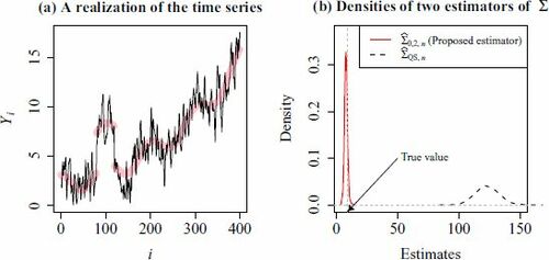Hence, the mean function (21) is a member of the class ${\mathcal{M}}^{⏧}$ defined in (20). Figure 1(a) shows a typical realization of $Y_i=X_i+{\mu }_i$ ($1\le i\le 400$). The density functions of ${\widehat{\Sigma }}_{0,2,n}$ and ${\widehat{\Sigma }}_{\text{QS},n}$ are shown in Figure 1(b). The proposed estimator ${\widehat{\Sigma }}_{0,2,n}$ concentrates at around the true value Σ = 9, however, the standard estimator ${\widehat{\Sigma }}_{\text{QS},n}$ is obviously off the targeted value.

Fig. 1 (a) A typical realization of the time series with the mean function defined in (21). (b) The density functions of ${\widehat{\Sigma }}_{0,2,n}$ and ${\widehat{\Sigma }}_{\text{QS},n}$ when n = 400. The true value is Σ = 9.

4.2 Comparison With Standard Estimators

The estimator ${\widehat{\mathbf{\Sigma }}}_{p,q,n}$ sacrifices statistical efficiency to gain robustness. In this section, we investigate how much efficiency is lost.

The proposed robust estimator ${\widehat{\mathbf{\Sigma }}}_{0,1,n}$ uses the Bartlett kernel $K_1(·)\equiv \text{Bart}(·)$. So, we compare it with the standard non-robust Bartlett kernel estimator ${\widehat{\mathbf{\Sigma }}}_{\text{Bart},n}$ defined in (4). Denote the optimal bandwidths for ${\widehat{\mathbf{\Sigma }}}_{0,1,n}$ and ${\widehat{\mathbf{\Sigma }}}_{\text{Bart},n}$ by ${\mathcal{l}}_{0,1}^{⏧}$ and ${\mathcal{l}}_{\text{Bart}}^{⏧}$, respectively. According to (15) and (17), and Equation (5.2) of Andrews (1991), they are given by$${\mathcal{l}}_{0,1}^{⏧}\sim {\left(\frac{3{\kappa }_{1}n}{2(1+c_1)}\right)}^{1/3}\hspace{1em}\text{and}\hspace{1em}{\mathcal{l}}_{\text{Bart}}^{⏧}\sim {\left(\frac{3{\kappa }_{1}n}{2}\right)}^{1/3},$$respectively, where κ₁ is defined in (18). Denote the resulting optimal estimators by ${\widehat{\mathbf{\Sigma }}}_{0,1,n}^{⏧}$ and ${\widehat{\mathbf{\Sigma }}}_{\text{Bart},n}^{⏧}$, respectively. The ratio of their weighted MSEs (see (16)) is given below.

Proposition 4.1. A

ssume the conditions in Theorems 3.1 and 3.2. Let $c_0,c_1>0,\mathit{W}\succ 0$, and $\mathit{\mu }(t)=\mathit{0}$ for all $t\in [0,1]$. Then ${\text{MSE}}_{\mathit{W}}({\widehat{\mathbf{\Sigma }}}_{0,1,n}^{⏧})/{\text{MSE}}_{\mathit{W}}({\widehat{\mathbf{\Sigma }}}_{\text{Bart},n}^{⏧})\to {(1+c_1)}^{2/3}>1$.

According to Proposition 4.1, the non-robust estimator ${\widehat{\mathbf{\Sigma }}}_{\text{Bart},n}^{⏧}$ is more efficient than the robust estimator ${\widehat{\mathbf{\Sigma }}}_{0,1,n}^{⏧}$ asymptotically. It makes sense. Note that the efficiency loss is smaller if c₁ is smaller. However, in finite sample, setting $c_1\approx 0$ may degenerate the estimator to the naive estimator ${\widehat{\mathbf{\Sigma }}}_{\text{naive},n}$ defined in (7). Hence, using a small $c_1>0$ is suggested only if the sample size n is extremely large. Practical suggestion on selecting c₁ is discussed in Section 4.3.

Besides, we also compare our estimator with the most promising (univariate) robust estimator proposed by Wu, Woodroofe, and Mentz (2001), Wu (2004), and Wu and Zhao (2007), namely,(22) $${\widehat{\sigma }}_{\text{WZ}3,n}^2:=\frac{\mathcal{l}}{2(m-1)}\sum _{k=2}^m{(A_k-A_{k-1})}^2,$$(22) where $m=\lfloor n/\mathcal{l}\rfloor$, and $A_k={\mathcal{l}}^{-1}{\sum }_{i=1+(k-1)\mathcal{l}}^{k\mathcal{l}}{Y}_i$ is the kth non-overlapping batch mean (NBM) for $k=1,\dots ,m$. The optimal MSE of ${\widehat{\sigma }}_{\text{WZ}3,n}^2$ was not derived by the authors. For reference, we derive it under the constant mean assumption. Applying similar techniques as in Theorems 3.1 and 3.2, we have $\text{Bias}({\widehat{\sigma }}_{\text{WZ}3,n}^2)\sim -{\Sigma }_1/\mathcal{l}$ and $\text{var}({\widehat{\sigma }}_{\text{WZ}3,n}^2)\sim 7{\Sigma }^2\mathcal{l}/(2n).$ The optimal bandwidth is $\mathcal{l}\sim {\{4{\Sigma }_1^{2}n/(7{\Sigma }^2)\}}^{1/3}$. Consequently, $\text{MSE}({\widehat{\Sigma }}_{0,1,n})/\text{MSE}({\widehat{\sigma }}_{\text{WZ}3,n}^2)\to {\left\{8(1+c_1)/21\right\}}^{2/3}$. In particular, when $c_1=1$, our estimator ${\widehat{\Sigma }}_{0,1,n}$ is uniformly better than ${\widehat{\sigma }}_{\text{WZ}3,n}^2$, and satisfies that $\text{MSE}({\widehat{\Sigma }}_{\text{Bart},n}):\text{MSE}({\widehat{\Sigma }}_{0,1,n}):\text{MSE}({\widehat{\sigma }}_{\text{WZ}3,n}^2)\approx 1.00:1.59:1.90$ when n is large and their respective optimal bandwidths are used.

4.3 Choices of q, c₀, c₁, and $\mathcal{l}$

The best estimator in Wu and Zhao (2007) has a MSE of size $O(n^{-2/3})$, whereas our proposed estimator ${\widehat{\mathbf{\Sigma }}}_{0,q,n}$ has a much smaller MSE, that is, $O\left\{n^{-2q/(1+2q)}\right\}$, if q > 1. In practice, if there is no prior information, we suggest q = 2, that is, assuming $\text{CSD}(\mathit{X})=2$, which is essentially equivalent to the assumption (${\Upsilon }_2<\infty$) made by Paparoditis and Politis (2001).

Although we develop theories for all $c_1>0$, it makes little sense to use $c_1\in (0,1)$ statistically and intuitively. To see it, observe that ${\widehat{\mathbf{\Pi }}}_k(L_k)={\widehat{\mathbf{\Psi }}}_{L_k}-{\widehat{\mathbf{\Psi }}}_{\left|k\right|}$ is a reasonable estimator of ${\mathbf{\Pi }}_k$ only if $L_k>\left|k\right|$, which is satisfied for all k if and only if $c_1\ge 1$. Hence, it is sensible (but not necessary) to assume $c_1\in [1,\infty )$, among which $c_1=1$ minimizes the AMSE. So, $c_1=1$ is suggested in practice. For q > 1, ${\widehat{\mathbf{\Sigma }}}_{p,q,n}$ has the same AMSE for any $c_0>0$, hence, c₀ does not affect the asymptotic behavior. We illustrate in Section C.4 of the supplementary materials that the finite sample performance of ${\widehat{\mathbf{\Sigma }}}_{p,q,n}$ is essentially the same for any c₀ that is not close to zero. In practice, we suggest using $c_0=1$ as a default choice.

If an initial pilot estimate of ${\mathbf{\Sigma }}_p$ is needed, we can use ${\widehat{\mathbf{\Sigma }}}_{p,q,n}$ with a rate optimal bandwidth $\mathcal{l}=O(n^{{\theta }^{⏧}})$. In practice, we suggest $\mathcal{l}=[\mathrm{}[2n^{{\theta }^{⏧}}]\mathrm{}]$, where $[\mathrm{}[t]\mathrm{}]:=(2\vee \lceil t\rceil )\wedge (n-1)$. According to our simulation experience, this rule-of-thumb bandwidth gives reasonably good performance. Using the notation in (10), we denote the resulting pilot estimator by(23) $${\widehat{\mathbf{\Sigma }}}_{p,q,n}^{†}:={\widehat{\mathbf{\Sigma }}}_{p,q,n}\left({\mathit{Y}}_{1:n},\mathcal{l}=\left[\mathrm{}\right[2n^{1/(1+2p+2q)}\left]\mathrm{}\right],c_0=1,c_1=1\right).$$(23)

In particular, for estimating $\mathbf{\Sigma }\equiv {\mathbf{\Sigma }}_0$, our recommended default estimator is as simple as(24) $${\widehat{\mathbf{\Sigma }}}_{0,2,n}^{†}=\sum _{k=-\mathcal{l}}^{\mathcal{l}}\left(1-{\left|\frac{k}{\mathcal{l}}\right|}^2\right)\left({\widehat{\mathbf{\Psi }}}_{\mathcal{l}+\left|k\right|}-{\widehat{\mathbf{\Psi }}}_{\left|k\right|}\right),$$(24) where $\mathcal{l}=[\mathrm{}[2n^{1/5}]\mathrm{}]$ and ${\widehat{\mathbf{\Psi }}}_h={\{2(n-\left|h\right|+1)\}}^{-1}{\sum }_{i=\left|h\right|+1}^n{({\mathit{Y}}_i-{\mathit{Y}}_{i-\left|h\right|})}^{\otimes 2}$. If a more accurate estimate of ${\mathbf{\Sigma }}_p$ is needed, we can use ${\widehat{\mathbf{\Sigma }}}_{p,q,n}$ with a fully optimal bandwidth $\mathcal{l}\sim {\varphi }^{⏧}{n}^{{\theta }^{⏧}}$. From (17), ${\varphi }^{⏧}$ is a function of $\mathbf{\Sigma }$ and ${\mathbf{\Sigma }}_{p+q}$. So, the value of ${\varphi }^{⏧}$ is unknown. We propose to first estimate $\mathbf{\Sigma }$ and ${\mathbf{\Sigma }}_{p+q}$ by the pilot estimators ${\widehat{\mathbf{\Sigma }}}_{0,2,n}^{†}$ and ${\widehat{\mathbf{\Sigma }}}_{p+q,2,n}^{†}$. Then ${\varphi }^{⏧}$ is consistently estimated by plugging in these estimated values into (17) and (18), that is,(25) $${\widehat{\varphi }}^{⏧}:={\left\{\mathrm{}\frac{\begin{array}{c}(2p+q+1)(2p+2q+1)\\ {(\text{vec}{\widehat{\Sigma }}_{p+q,2,n}^{†})}^{⊺}\mathcal{W}(\text{vec}{\widehat{\Sigma }}_{p+q,2,n}^{†})\end{array}}{\begin{array}{c}2q(1+c_1){(\text{vec}{\widehat{\mathbf{\Sigma }}}_{0,1,n}^{†})}^{⊺}\mathcal{W}(\text{vec}{\widehat{\mathbf{\Sigma }}}_{0,2,n}^{†})\\ +\text{tr}\{\mathcal{W}({\widehat{\mathbf{\Sigma }}}_{0,2,n}^{†}\otimes {\widehat{\mathbf{\Sigma }}}_{0,2,n}^{†})\}\end{array}}\mathrm{}\right\}}^{\mathrm{}1/(1+2p+2q)}.$$(25)

Using ${\widehat{\mathcal{l}}}^{⏧}:=[\mathrm{}[{\widehat{\varphi }}^{⏧}{n}^{{\theta }^{⏧}}]\mathrm{}],$ the estimator ${\widehat{\mathbf{\Sigma }}}_{p,q,n}$ is equipped with the optimal bandwidth asymptotically. The resulting estimator(26) $${\widehat{\mathbf{\Sigma }}}_{p,q,n}^{‡}:={\widehat{\mathbf{\Sigma }}}_{p,q,n}\left({\mathit{Y}}_{1:n},\mathcal{l}=\left[\mathrm{}\right[{\widehat{\varphi }}^{⏧}{n}^{1/(1+2p+2q)}\left]\mathrm{}\right],c_0=1,c_1=1\right)$$(26) is called the qth order MAC estimator of ${\mathbf{\Sigma }}_p$. It can be computed by Algorithm 1. The R-package MAC is built for implementing it.

Algorithm 1: Proposed MAC estimator ${\widehat{\mathbf{\Sigma }}}_{p,q,n}^{‡}$ for estimating ${\mathbf{\Sigma }}_p$

[1] Input:

[2] (i) ${\mathit{Y}}_{1:n}$—d-dimensional time series;

[3] (ii) p—order of the estimand ${\mathbf{\Sigma }}_p$ (set p = 0 for estimation of the ACM $\mathbf{\Sigma }$);

[4] (iii) q—order of the polynomial kernel $K_q(·)$ (set q = 2 by default);

[5] (iv) c₀, c₁—parameters (set $c_0=c_1=1$ by default); and

[6] (v) W—d × d weight matrix (set $W^{[r,s]}=1\{r\le s\}$ for each $1\le r,s\le d$ by default).

[7] begin

[8] Compute ${\widehat{\mathbf{\Sigma }}}_{0,2,n}^{†}$ and ${\widehat{\mathbf{\Sigma }}}_{p+q,2,n}^{†}$ according to (23);

[9] Compute ${\widehat{\varphi }}^{⏧}$ according to (25);

[10] Compute the estimated optimal bandwidth ${\widehat{\mathcal{l}}}^{⏧}=[\mathrm{}[{\widehat{\varphi }}^{⏧}{n}^{1/(1+2p+2q)}]\mathrm{}]$;

[11] Compute ${\widehat{\mathbf{\Sigma }}}_{p,q,n}^{‡}={\widehat{\mathbf{\Sigma }}}_{p,q,n}({\mathit{Y}}_{1:n},\mathcal{l}={\widehat{\mathcal{l}}}^{⏧},c_0,c_1)$ according to (10).

return ${\widehat{\mathbf{\Sigma }}}_{p,q,n}^{‡}$ – MAC estimator of ${\mathbf{\Sigma }}_p$.

4.4 Discussion on Robustness to Heteroscedasticity

Thus far we have assumed that the noise sequence $\left\{{\mathit{X}}_i\right\}$ is stationary (i.e., without heteroscedasticity). Now, suppose that $\left\{{\mathit{X}}_i\right\}$ is not stationary but satisfies $\mathrm{E}({\mathit{X}}_i)=0$. In this case, we define the finite-n version of ${\mathbf{\Sigma }}_0=\underset{n\to \infty }{\lim }n\text{var}({\overline{\mathit{Y}}}_n)$ by(27) $$\begin{array}{c}{\mathbf{\Sigma }}_{0,n}:=n\text{var}\left({\overline{\mathit{Y}}}_n\right)=n\mathrm{E}\left({\overline{\mathit{X}}}_n{\overline{\mathit{X}}}_n^{⊺}\right)\\ =\frac{1}{n}\underset{1\le i,j\le n}{\sum \sum }\mathrm{E}\left({\mathit{X}}_i{\mathit{X}}_j^{⊺}\right)=\sum _{\left|k\right|<n}{\mathbf{\Pi }}_{k,n},\end{array}$$(27) where ${\mathbf{\Pi }}_{k,n}={\sum }_{i=1+\left|k\right|}^n\mathrm{E}(X_i{X}_{i-\left|k\right|}^{⊺}+X_{i-\left|k\right|}{X}_i^{⊺})/(2n)$. Following the arguments in Section 3.1, it is not hard to see that ${\widehat{\mathbf{\Pi }}}_k(L)$ still approximates ${\mathbf{\Pi }}_{k,n}$. Thus, it is not surprising that the proposed estimator ${\widehat{\mathbf{\Sigma }}}_{p,q,n}$ continues to be consistent for ${\mathbf{\Sigma }}_{p,n}:=\sum _{\left|k\right|<n}|k{|}^p{\mathbf{\Pi }}_{k,n}$. Similar to Section 8 of Andrews (1991), we can extend the consistency results to heteroscedastic time series. Suppose the regularity conditions of Theorem 4.1, Theorem 4.2, and part (1) of Corollary 4.1 are satisfied except the following changes.

• The stationarity of the noise sequence $\left\{{\mathit{X}}_i\right\}$ is removed. However, it still satisfies that there is some $\nu >4$ such that ${\mathit{X}}_i\in {\mathcal{L}}^{\nu }$ and $\mathrm{E}({\mathit{X}}_i)=\mathit{0}$ for all $i\in \mathbb{Z}$.

• The assumption $\text{CSD}(\mathit{X})=p+q$ is changed to ${\text{CSD}}_{*}(\mathit{X})=p+q$, where$$\begin{array}{c}{\text{CSD}}_{*}(\mathit{X}):=\sup \\ \hspace{1em}\left\{P\in \mathbb{N}:\underset{{}_{r,s\in \{1,\dots ,d\}}}{\max }\sum _{k=-\infty }^{\infty }|k{|}^P\underset{i\ge 1}{\sup }\mathrm{E}(X_i^{\left[r\right]}{X}_{i-k}^{\left[s\right]})<\infty \right\}.\end{array}$$

We also define, for each $P\in {\mathbb{N}}_0$, that$$\begin{array}{c}{\Sigma }_{P,*}^{[r,s]}:=\sum _{k=-\infty }^{\infty }|k{|}^P\underset{i\ge 1}{\sup }\mathrm{E}(X_i^{\left[r\right]}{X}_{i-k}^{\left[s\right]})\hspace{1em}\text{and}\\ \hspace{1em}{\Xi }_{*}^{[r,s]}:={\Sigma }_{0,*}^{[r,r]}{\Sigma }_{0,*}^{[s,s]}+{\left({\Sigma }_{0,*}^{[r,s]}\right)}^2.\end{array}$$

Note that ${\text{CSD}}_{*}(\mathit{X})=P$ implies that ${\Sigma }_{P,*}^{[r,s]}<\infty$ and ${\Xi }_{*}^{[r,s]}<\infty$ for each r, s. Under the modified regularity conditions, the conclusions of Theorems 4.1 and 4.2 are updated to(28) $$\underset{n\to \infty }{\lim \sup }{\mathcal{l}}^{2q}{\left\{\mathrm{E}\left({\widehat{\Sigma }}_{p,q,n}^{[r,s]}\right)-{\Sigma }_{p,n}^{[r,s]}\right\}}^2\le {\left({\Sigma }_{p+q,*}^{[r,s]}\right)}^2,$$(28) (29) $$\begin{array}{c}\underset{n\to \infty }{\lim \sup }\frac{n}{{\mathcal{l}}^{1+2p}}\text{var}\left({\widehat{\Sigma }}_{p,q,n}^{[r,s]}\right)\\ \hspace{1em}\le \frac{4q^2\left(1+c_1\right){\Xi }_{*}^{[r,s]}}{(2p+1)(2p+q+1)(2p+2q+1)}\end{array}$$(29)

for all $r,s\in \{1,\dots ,d\}$. If $\mathcal{l}=O(n^{1/(1+2p+2q)})$, then (28) and (29) imply that$$\underset{n\to \infty }{\lim \sup }{n}^{2q/(1+2p+2q)}\mathrm{E}{\left({\widehat{\Sigma }}_{p,q,n}^{[r,s]}-{\Sigma }_{p,n}^{[r,s]}\right)}^2\le C$$for some $C<\infty$. Hence, ${\widehat{\mathbf{\Sigma }}}_{p,q,n}$ is a consistent estimator of ${\mathbf{\Sigma }}_{p,n}$ with the optimal convergence rate. Examples and finite-sample performance of ${\widehat{\mathbf{\Sigma }}}_{p,q,n}$ in the heteroscedastic case are shown in Section 5.3.

5 Finite Sample Performance

5.1 Efficiency and Robustness Against One Jump

We compare ${\widehat{\mathbf{\Sigma }}}_{0,q,n}$ with the following estimators in terms of efficiency and robustness.

• (CV) Crainiceanu and Vogelsang (2007) proposed to estimate one potential CP D₁ and then construct a de-trended process, say $\left\{{\widehat{X}}_i^{\text{CV}}\right\}$. The modified OBM estimator ${\widehat{\sigma }}_{\text{CV},n}^2$ is defined by applying the estimator (3) to $\left\{{\widehat{X}}_i^{\text{CV}}\right\}$ instead of $\left\{{\widehat{X}}_i\right\}$. Andrews (1991)’s AR(1)-plug-in rule is used for selecting the optimal batch size.

• (WZ) Wu and Zhao (2007) used NBMs $\left\{A_k\right\}$ to estimate ${\sigma }^2$. They proposed ${\widehat{\sigma }}_{\text{WZ}1,n}^2:=\pi \mathcal{l}{\left\{4{(m-1)}^2\right\}}^{-1}{\sum }_{k=2}^m|A_k-A_{k-1}|,{\widehat{\sigma }}_{\text{WZ}2,n}^2:=\mathcal{l}{(2z_{3/4})}^{-1}\underset{k\in \{2,\dots ,m\}}{\text{median}}|A_k-A_{k-1}|$, and ${\widehat{\sigma }}_{\text{WZ}3,n}^2$ defined in (22), where $\underset{k\in \mathcal{K}}{\text{median}}{x}_k$ denotes the median of ${\left\{x_k\right\}}_{k\in \mathcal{K}}$, and z_p is the $100p\%$ quantile of $\mathcal{N}(0,1)$. They showed, under regularity conditions, that ${\widehat{\sigma }}_{\text{WZ}1,n}^2$ and ${\widehat{\sigma }}_{\text{WZ}2,n}^2$ are weakly consistent if $\mathcal{l}=[\mathrm{}[n^{5/8}]\mathrm{}]$, and that ${\widehat{\sigma }}_{\text{WZ}2,n}^2$ is ${\mathcal{L}}^2$ consistent with $\text{MSE}({\widehat{\sigma }}_{\text{WZ}3,n}^2)=O(n^{-2/3})$ if $\mathcal{l}\asymp n^{1/3}$. For ${\widehat{\sigma }}_{\text{WZ}3,n}^2$, we implement it with the an estimated optimal bandwidth by using our proposed estimator (see Section 4.2 for more details). Denote these three estimators by WZ1, WZ2, and WZ3, respectively.

• (AC) Altissimoa and Corradic (2003) proposed using Bartlett kernel estimator after locally detrending the mean. The bandwidth is selected by cross-validation. Denote the resulting estimator by ${\widehat{\sigma }}_{\text{AC},n}^2$. They proved that ${\widehat{\sigma }}_{\text{AC},n}^2$ is consistent (see Table 1).

• (MAC) We use the estimators ${\widehat{\Sigma }}_{0,1,n}^{‡}$ and ${\widehat{\Sigma }}_{0,2,n}^{‡}$, as well as the pilot estimator ${\widehat{\Sigma }}_{0,2,n}^{†}$. Denote them by MAC(1), MAC(2), and MAC(P), respectively.

Their detailed formulas are presented in Section C.1 of the supplementary materials for reference. We recall from Table 1 that ${\widehat{\sigma }}_{\text{CV},n}^2$ is robust to one CP without trend; ${\widehat{\sigma }}_{\text{WZ}1,n}^2$, ${\widehat{\sigma }}_{\text{WZ}2,n}^2$ and ${\widehat{\sigma }}_{\text{WZ}3,n}^2$ are proved to be robust to trends only; ${\widehat{\sigma }}_{\text{AC},n}^2$ is only proved to be robust to finitely many CPs; and the proposed estimators ${\widehat{\Sigma }}_{0,1,n}^{⏧}$ and ${\widehat{\Sigma }}_{0,2,n}^{⏧}$ are robust to both trends and a divergent number of CPs. If there is at most one CP, then ${\widehat{\sigma }}_{\text{CV},n}^2$ is an oracle estimator because, in practice, we rarely know that there is at most one CP.

Consider the ARMA(1,1) model: $Y_i=X_i+{\mu }_i$ where $X_i=a{X}_{i-1}+b{\epsilon }_{i-1}+{\epsilon }_i$ and ${\epsilon }_i\stackrel{\text{iid}}{\sim }\mathcal{N}(0,1)$, for $i=1,\dots ,n$. In particular, consider $a=b=0.2,0.4,0.6$ (Models A1–A3, respectively), $n=400\times 4^j,j=0,\dots ,3$, and five different mean sequences ${\mu }_i=\xi \times 1\{i\le n/2\}$ for $\xi =0,\dots ,4$. The MSEs are estimated by using 2000 independent replications. The lack of efficiency (${\text{MSE}}_0$) is measured by the MSE when ξ = 0, whereas the lack of robustness is measured by the standard derivation (${\text{MSE}}_{\text{sd}}$) of the MSEs across $\xi \in \{0,1,\dots ,4\}$. Smaller ${\text{MSE}}_0$ and smaller ${\text{MSE}}_{\text{sd}}$ imply higher efficiency and robustness, respectively.

The results are shown in Figure 2. Clearly, ${\widehat{\sigma }}_{\text{WZ}1,n}^2$ and ${\widehat{\sigma }}_{\text{WZ}2,n}^2$ perform badly in terms of both efficiency and robustness. The major competitor ${\widehat{\sigma }}_{\text{WZ}3,n}^2$ performs reasonably well in terms of both two measures, however, it is less efficient than all of our proposed estimators (${\widehat{\Sigma }}_{0,1,n}^{‡}$, ${\widehat{\Sigma }}_{0,2,n}^{‡}$, ${\widehat{\Sigma }}_{0,2,n}^{†}$) in nearly all cases. The estimator ${\widehat{\sigma }}_{\text{AC},n}^2$ is quite efficient when the mean is a constant, however, it loses all of its efficiency when the jump size is large. For example, when n = 400, its MSE inflates 407% when the jump magnitude ξ increases from 0 to 4. Besides, the cross-validation step makes it computationally inefficient.

Fig. 2 The values of $\text{log}\hspace{0.17em}({\text{MSE}}_0)$ and $\text{log}\hspace{0.17em}({\text{MSE}}_{\text{sd}})$ are plotted against n, where ${\text{MSE}}_0$ denotes the MSE when the jump size ξ = 0, and ${\text{MSE}}_{\text{sd}}$ denotes the standard deviation of the MSEs across different ξ. Recall that smaller ${\text{MSE}}_0$ and smaller ${\text{MSE}}_{\text{sd}}$ imply higher efficiency and robustness, respectively. Note that ${\widehat{\sigma }}_{\text{AC},n}^2$ is computed only when $n\le 400$ because it requires a computationally intensive cross-validation step. Note that horizontal axis is plotted in the logarithmic scale for better visualization.

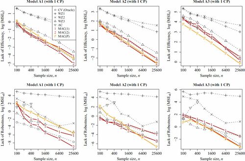
The proposed estimators ${\widehat{\Sigma }}_{0,1,n}^{‡}$ and ${\widehat{\Sigma }}_{0,2,n}^{‡}$ perform the best in nearly all cases. The advantage of ${\widehat{\Sigma }}_{0,2,n}^{‡}$ is increasingly obvious when n increases. The pilot estimator ${\widehat{\Sigma }}_{0,2,n}^{†}$ performs quite well, so it is justifiable to use it as an initial guess. It is remarked that ${\widehat{\Sigma }}_{0,2,n}^{†}$ performs very well in Model A3 because its default tuning parameter accidentally matches the theoretically optimal value. However, this privilege is not general (see, e.g., Figure 5 of another experiment in Section 5.3).

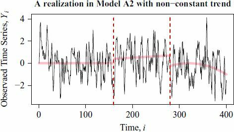
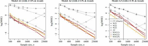
5.2 Robustness Against Trend and Multiple Jumps

In this subsection, we investigate the robustness against both trends and jumps. Consider the same models of $\left\{X_i\right\}$ in Section 5.1, but the mean function is replaced by ${\mu }_i=(i/n)\mathrm{}1\{0.4\le i/n<0.7\}+{(5i/n-4)}^2\mathrm{}1\{i/n\ge 0.7\}$. Figure 3 shows a typical realization of $\left\{Y_i\right\}$ in Model A2. Observe that the trend effect and jump effect are not obvious because they are masked by the intrinsic variability of the noises $\left\{X_i\right\}$. This scenario mimics the situation in which the observed time series looks stationary but, indeed, it has been contaminated by a hardly noticeable nonconstant trend and structural breaks.

Fig. 3 Thin solid line: A realization of $\left\{Y_i\right\}$ in Model A2 of length n = 400. Thick solid line: The nonconstant mean function $\left\{{\mu }_i\right\}$ in Section 5.2. Dotted vertical lines: The change points.

The simulation result is visualized in Figure 4. First, the MSE of the previous oracle estimator ${\widehat{\sigma }}_{\text{CV},n}^2$ does not decrease with n because it is no longer consistent when the mean is not a piecewise constant function. The estimators ${\widehat{\sigma }}_{\text{WZ}1,n}^2$ and ${\widehat{\sigma }}_{\text{WZ}2,n}^2$ perform poorly again. The estimator ${\widehat{\sigma }}_{\text{WZ}3,n}^2$ and our proposed ${\widehat{\Sigma }}_{0,1,n}^{‡}$, ${\widehat{\Sigma }}_{0,2,n}^{‡}$, ${\widehat{\Sigma }}_{0,2,n}^{†}$ perform well. Among them, ${\widehat{\sigma }}_{\text{WZ}3,n}^2$ performs least well, whereas ${\widehat{\Sigma }}_{0,2,n}^{‡}$ and ${\widehat{\Sigma }}_{0,2,n}^{†}$ perform most promisingly. The take-home message is that even if the trend is relatively insignificant, the impact on the estimators of ${\sigma }^2$ can be catastrophic especially when the mean-structure is misspecified.

Fig. 4 The values of $\text{log}\hspace{0.17em}\left\{\text{MSE}(·)\right\}$ of different estimators are plotted against the sample size n in Models A1–A3. Here the mean function consists of nonconstant trends and multiple jumps (see Section 5.2 and Figure 3). Note that horizontal axis is plotted in the logarithmic scale.

5.3 Multivariate Time Series With Heteroscedastic Errors

We consider estimation of ${\mathbf{\Sigma }}_{0,n}$ (defined in (27)) for a bivariate time series ${\{{\mathit{Y}}_i={(Y_{i1},Y_{i2})}^{⊺}\}}_{i=1}^n$ with time-varying means and heteroscedastic errors. Let $Y_{ij}={\mu }_{ij}+{\tau }_{ij}{X}_{ij}$ for $i=1,\dots ,n$ and j = 1, 2, where μ_ij is the mean, X_ij is a stationary noise, and τ_ij creates heteroscedasticity. Two mean sequences are used: (i) ${\mu }_{ij}=0$ for all i, j, and (ii) ${\mu }_{i1}=i/n,{\mu }_{i2}=1(i/n>1/3)$. We set ${\tau }_{i1}=1+i/(4n),{\tau }_{i2}=1+\hspace{0.17em}\text{sin}\hspace{0.17em}(4\pi i/n)/(4n)$, and generate $\left\{X_{ij}\right\}$ as follows:$$\begin{array}{c}\left[\begin{array}{c}{X}_{i1}\\ X_{i2}\end{array}\right]=\left[\begin{array}{cc}0.27& -0.09\\ -0.18& 0.18\end{array}\right]\left[\begin{array}{c}{X}_{i-1,1}\\ X_{i-1,2}\end{array}\right]\\ \hspace{1em}+\left[\begin{array}{cc}0.01& -0.14\\ 0.28& 0.08\end{array}\right]{\mathit{\epsilon }}_{i-1}+{\mathit{\epsilon }}_i,\hspace{1em}i=1,2,\dots ,n,\end{array}$$where ${\mathit{\epsilon }}_0,\dots ,{\mathit{\epsilon }}_n$ are independent standard bivariate normal random vectors.

The proposed estimators ${\widehat{\mathbf{\Sigma }}}_{0,1,n}^{‡}$, ${\widehat{\mathbf{\Sigma }}}_{0,2,n}^{‡}$, and ${\widehat{\mathbf{\Sigma }}}_{0,2,n}^{†}$ are evaluated. We compare them with the standard Bartlett kernel estimator ${\widehat{\mathbf{\Sigma }}}_{\text{Bart},n}$ and QS kernel estimators ${\widehat{\mathbf{\Sigma }}}_{\text{QS},n}$ (see (4)). The bandwidths of ${\widehat{\mathbf{\Sigma }}}_{\text{Bart},n}$ and ${\widehat{\mathbf{\Sigma }}}_{\text{QS},n}$ are selected by Andrews’s (1991) vector AR(1)-plug-in rule. As far as we know, in the multivariate setting, there exists no other estimator that is proved to be consistent and optimal in the presence of nonconstant mean, autocorrelation and heteroscedasticity. The results are shown in Figure 5. We also repeat the experiment with homoscedastic errors, that is, ${\tau }_{ij}=1$ for all i, j. Since the results are very similar to the heteroscedastic case, we only present the result in Figure 3 of the supplementary materials.

Fig. 5 The values of $\text{log}\hspace{0.17em}\left\{{\text{MSE}}_{\mathit{W}}(·)\right\}$ for ${\widehat{\mathbf{\Sigma }}}_{\text{Bart},n}$, ${\widehat{\mathbf{\Sigma }}}_{\text{QS},n},{\widehat{\mathbf{\Sigma }}}_{0,1,n}^{‡}$, ${\widehat{\mathbf{\Sigma }}}_{0,2,n}^{‡}$ and ${\widehat{\mathbf{\Sigma }}}_{0,2,n}^{†}$ in the heteroscedastic case are plotted against n, where $\text{vec}(\mathit{W})={(1,1/2,1/2,1)}^{⊺}$ is used, and ${\text{MSE}}_{\mathit{W}}(·)$ is defined in (16). The left and right plots show the results in the constant mean and nonconstant mean cases, respectively. Note that the horizontal axes are plotted in the logarithmic scale.

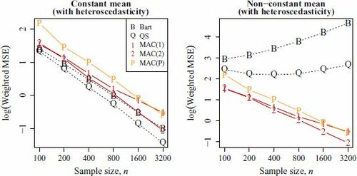
From Figure 5, all five estimators are consistent in the constant-mean case. However, ${\widehat{\mathbf{\Sigma }}}_{\text{Bart},n}$ and ${\widehat{\mathbf{\Sigma }}}_{\text{QS},n}$ are no longer consistent when the mean is not a constant. On the other hand, the mean-structure does not affect the performance of ${\widehat{\mathbf{\Sigma }}}_{0,1,n}^{‡}$, ${\widehat{\mathbf{\Sigma }}}_{0,2,n}^{‡}$, and ${\widehat{\mathbf{\Sigma }}}_{0,2,n}^{†}$. It verifies the claimed consistency and robustness. In addition, although the pilot estimator ${\widehat{\mathbf{\Sigma }}}_{0,2,n}^{†}$ does not perform as well as the optimal estimator ${\widehat{\mathbf{\Sigma }}}_{0,2,n}^{‡}$, it is still able to give sufficiently good results. It supports the use of ${\widehat{\mathbf{\Sigma }}}_{0,2,n}^{†}$ as an initial estimator in practice.

5.4 Change-Point Detection

In this subsection, we consider the CP detection problem, that is, to test $H_0:\mathrm{E}{Y}_1=\cdots =\mathrm{E}{Y}_n$ against $H_1:\exists D_1\text{such}\mathrm{}\text{that E}{Y}_1=\cdots =\mathrm{E}{Y}_{D_1-1}\ne \mathrm{E}{Y}_{D_1}=\cdots =\mathrm{E}{Y}_n$. We analyze (i) whether CP tests are monotonically powerful with respect to the magnitude of jump $|\mathrm{E}{Y}_{D_1}-\mathrm{E}{Y}_{D_1-1}|$; and (ii) their power losses under a misspecified alternative hypothesis.

Let $T_n(k):=n^{-1/2}{\sum }_{i=1}^k{\widehat{X}}_i$ be the CUSUM process of ${\widehat{X}}_i=Y_i-{\overline{Y}}_n$. The standard KS test statistic is defined by $T_n:={\max }_{k\in \{1,\dots ,n\}}\left|T_n(k)/\widehat{\sigma }\right|$, where $\widehat{\sigma }$ is a consistent estimator of σ. Then, H₀ is rejected at 5% level if $T_n>1.358$. Alternatively, a self-normalized KS test (Shao and Zhang 2010) can be used. Following them, we compare

• (SZ) their self-normalized KS test, and

• (KS) the standard KS tests with different estimators of ${\sigma }^2$, namely, ${\widehat{\sigma }}_{\mathrm{A},n}^2$, ${\widehat{\sigma }}_{\text{CV},n}^2$ ${\widehat{\sigma }}_{\text{JX},n}^2$, ${\widehat{\sigma }}_{\text{WZ}3,n}^2$, ${\widehat{\sigma }}_{\text{AC},n}^2$, and ${\widehat{\Sigma }}_{0,2,n}^{‡}$, where ${\widehat{\sigma }}_{\mathrm{A},n}^2$ is Bartlett kernel estimator with Andrew’s AR(1) plug-in selector of $\mathcal{l}$; the estimator ${\widehat{\sigma }}_{\text{JX}}^2$ is proposed by Juhl and Xiao (2009); and all other estimators are defined in Section 5.1.

Detailed formulas of the above CP tests and estimators of ${\sigma }^2$ are presented in Section C.3 of the supplementary materials for reference. Consider the bilinear model: $Y_i=X_i+{\mu }_i$ where $X_i=(a+b{\epsilon }_i)X_{i-1}+{\epsilon }_i$ and ${\epsilon }_i\stackrel{\text{iid}}{\sim }\mathcal{N}(0,1)$, for $i=1,\dots ,n$. The physical dependence measure decays at the rate ${\delta }_{4,n}^{[1]}=O({\varrho }^n)$, where $\varrho =\sqrt{a^2+b^2}$ (see Wu 2005, 2011). If ϱ is larger, the serial dependence is stronger. We use $a=0.33,0.36,0.39$ and $b=0.5,0.6,0.7$ so that $\varrho =0.6,0.7,0.8$, respectively. Denote them by Models B1–B3, respectively.

Both SZ and KS tests assume that the mean function is a piecewise constant with one CP when H₀ is false. If it is actually the case, we call that the alternative hypothesis is correctly specified, otherwise, the alternative hypothesis is said to be misspecified. We consider the following two alternative hypotheses in the experiments:

• (correctly specified alternative) H₁: ${\mu }_i=\xi \times \mathrm{}1\{i/n>1/4\}$ for $i=1,\dots ,n$; and

• (misspecified alternative) $H_1^{\prime }$: ${\mu }_i=\xi (1+e^{-10i/n+5})\times \mathrm{}1\{i/n>1/4\}$ for all $i=1,\dots ,n$,

where the value of $\xi \in \mathbb{R}$ controls the jump magnitude. If ξ = 0, both H₁ and $H_1^{\prime }$ reduce to H₀. In H₁, the mean jumps to ξ at $i=\lfloor n/4\rfloor +1$, and then stays constant; whereas, in $H_1^{\prime }$, the mean shoots up at $i=\lfloor n/4\rfloor +1$, and then decays to ξ. In practice, CP may arrive like $H_1^{\prime }$ instead of H₁, hence, a good CP test should be powerful in both cases. A good size-α CP test should satisfy the following four properties, where $\alpha \in (0,1)$.

• (Size correctness) The probability of rejecting H₀ is close to α when H₀ is correct.

• (Powerfulness) The probability of rejecting H₀ is high when H₀ is incorrect.

• (Monotonicity of power) The power is increasing with the magnitude of jump $\left|\xi \right|$.

• (Robustness) The test is still powerful under misspecified alternative hypotheses.

The simulation is conducted for n = 100, 400, 800 with nominal size $\alpha =5\%$. Since the results are similar under different models, we only report the results under Model B2 here (see Figure 6). The full results are deferred to Section C.3 in the supplementary materials. The size-adjusted power curves are also presented in the supplementary materials for reference. Under H₁, all tests except KS(A) and KS(JX) have monotonic powers with respect to $\left|\xi \right|$. The test KS(WZ3) commits the Type I error more frequently than the nominal value even when the sample size is large. This over-size phenomenon is due to the use of inefficiency estimator of ${\sigma }^2$. The power curves are largely the same for KS(CV), KS(AC), and KS(MAC(2)) as they are essentially the same test. Observe that SZ is significantly less powerful when $0<\xi <1$.

Fig. 6 The powers of the CP tests defined in Section 5.4 are plotted against the jump magnitude ξ under Model B2. The scenarios under well-specified alternative H₁ and misspecified alternative $H_1^{\prime }$ are shown in the upper and lower plots, respectively. Dashed horizontal lines indicate the significance level $\alpha =5\%$ and zero. Note that horizontal axis is plotted in the logarithmic scale for better visualization.

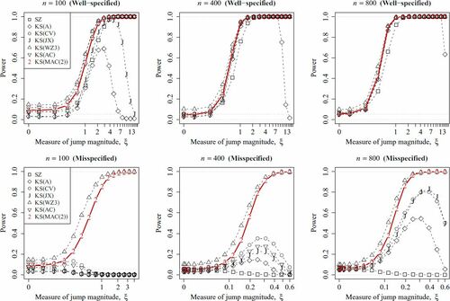
Under $H_1^{\prime }$, all tests except KS(MAC(2)) and KS(WZ(3)) immediately lose all power when $\left|\xi \right|>0$. In particular, SZ remains powerless even when n and ξ are large. It is not desirable because SZ is very sensitive to whether the alternative hypothesis is well-specified. For KS(A), KS(CV), KS(JX), and KS(AC), they are not powerfully because of using inconsistent or inefficient estimators of ${\sigma }^2$. It gives a sign of warning to use these tests in practice. It is worth emphasizing that KS(WZ3) seems more powerful than KS(MAC(2)). However, it is just because KS(WZ3) rejects too frequently no matter H₀ is true or not. Hence, the apparently more powerful KS(WZ3) test is not reliable. Among all tests above, our proposed test KS(MAC(2)) is the only monotonically powerful test that has accurate size and is insensitive to misspecification of the alternative hypothesis.

6 Empirical Studies

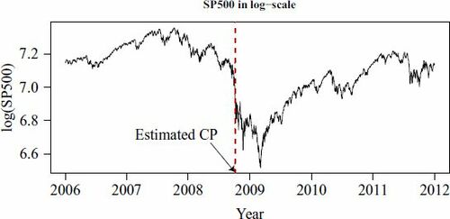
6.1 Change Point Detection in S&P 500 Index

The Standard & Poor’s 500 (S&P 500) Index is a stock market index based on 500 representative companies in the USA. The daily adjusted close prices of the index, from 3 January 2006 to 30 December 2011 (n = 1511), are investigated. The dataset can be downloaded from http://finance.yahoo.com/quote/%5EGSPC/history. The financial crisis in 2008 is believed to have a tremendous impact on the global stock market. We suspect that it led to an abrupt change in the stock market. Testing this claim is important since a noncontinuous impact implies that the economy may have a structural change.

Denote the logarithm of the S&P 500 Index by Y_i. Observe that there is an obvious trend in Y_i (see Figure 7). A standard approach is to study the return series $y_i:=Y_i-Y_{i-1}$ to get rid of the trend component. This differencing step is essential for many standard CP tests, for example, SZ and KS tests presented in Section 5.4, because they cannot handle trends. Using the CUMSUM-type CP estimator ${\widehat{D}}_1$ (see (1) of the supplementary materials for its formula), we estimate the CP to be 10 March 2009. It is remarked that the same CP is detected by the method described in Altissimoa and Corradic (2003). Hence, the CP test fails to capture the 2008 financial crisis. Indeed, testing H₀: “$\mathrm{E}{y}_1=\cdots =\mathrm{E}{y}_n$” by the KS(MAC) test defined in Section 5.4, we fail to reject H₀ at 5% level. We conclude that the 2008 financial crisis has no jump impact on the return y_i. Since taking the difference of Y_i may cancel out the potential jump effect, it seems desirable to analyze Y_i directly (see Vogelsang 1999 for a similar analysis). Using the CP test proposed by Wu and Zhao (2007), we can test H₀: “The mean function $i\mapsto \mathrm{E}{Y}_i$ is continuous” against H₁: “The mean function $i\mapsto \mathrm{E}{Y}_i$ has a jump-discontinuity.” The test statistic is $Q_n:={(k_n\widehat{\sigma })}^{-1}{\max }_{k_n\le i\le n-k_n}\left|{\sum }_{j=i+1}^{k_n+i}{Y}_j-{\sum }_{j=i-k_n+1}^i{Y}_j\right|,$ where ${\widehat{\sigma }}^2$ is a consistent estimator of ${\sigma }^2$, that is, the AVC of $\left\{Y_i\right\}$; and $k_n=\lfloor n^{0.6}\rfloor$. Then H₀ is rejected if Q_n is large. Using MAC(2) to estimate σ, we obtain $\widehat{\sigma }=0.0517$; and found that H₀ is rejected at any reasonable level. It is remarked that σ is estimated to be 0.0434 by using the estimator WZ3. Although this estimate is a bit smaller than our proposed estimate, the same conclusion for testing H₀ is obtained if this estimate is used in the test statistic Q_n. Although Wu and Zhao (2007) did not provide any estimator of the CP, they argue that if i + 1 is a discontinuity point, then the difference of the averages inside the statistic Q_n should be large. Following their idea, ${\widehat{D}}_{\text{WZ}}:=1+\underset{k_n\le i\le n-k_n}{\arg \max }\left|{\sum }_{j=i+1}^{k_n+i}{Y}_j-{\sum }_{j=i-k_n+1}^i{Y}_j\right|$ is a reasonable estimator of the CP. The estimated CP, ${\widehat{D}}_{\text{WZ}}$, is 7 October 2008 (see Figure 7). It indicates the 2008 financial crisis quite accurately. It coincides with our understanding of the stock market.

Fig. 7 Time series plot of $\left\{Y_i\right\}$, that is, the daily S&P 500 Index (3 January 2006–30 December 2011) in the log scale (see Section 6.1). The vertical dotted line indicates the value of ${\widehat{D}}_{\text{WZ}}$ estimated by the statistic in Wu and Zhao (2007). Here ${\sigma }^2$ is estimated by MAC(2).

6.2 Simultaneous Change Point Detection in Several Indices

Besides S&P 500 Index mentioned in Section 6.1, there are several other stock market indices that are commonly used by traders, for example, Dow Jones Index, Nasdaq Composite, and Russell 2000. In this subsection, we investigate whether we can make use of these four market indices simultaneously to make a more precise detection of the 2008 financial crisis.

Consider the squared daily returns, which can be used as proxies for daily volatilities, of the aforementioned four indices in the period 1 July 2008–30 December 2008 (see Figure 8). Applying the CUSUM-type CP estimator ${\widehat{D}}_1$ (see (1) of the supplementary materials for its formula) to each index individually, we obtain the same CP 29 September 2018. It is remarked that the no CP null hypothesis is rejected at 5% level by the test KS(MAC(2)) for each individual index.

Fig. 8 The squared returns of four stock indices (1 July 2008–30 December 2008) (see Section 6.2). The two vertical lines denote the CP locations. The earlier and later CPs are detected by the multivariate and univariate CUSUM CP estimators, respectively.

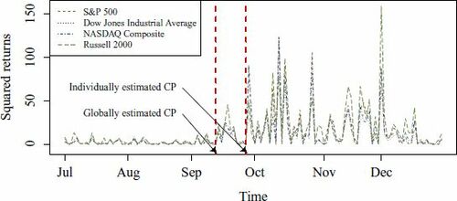
Since these stock market indices are highly correlated and are believed to follow the market trend very closely, a CP (if any) is likely to appear simultaneously. Hence, using multivariate time series for detecting a CP can be more accurate and precise. Applying the multivariate version of the KS CP test (Horváth, Kokoszka, and Steinebach 1999) to the four indices, we detect the CP to be 15 September 2008. From Figure 8, the squared returns between 15 and 29 September are slightly higher than the first portion of the series. Hence, using multivariate time series helps detecting these small changes. Consequently, multivariate tests are potentially more useful in practice. It is also remarked that the no simultaneous CP alternative is rejected at 5% level by the CP test (Horváth, Kokoszka, and Steinebach 1999) with our proposed MAC(2) estimator.

7 Conclusions

In this article, we propose an estimator of the ACM in nonstationary time series. The estimator has several desirable features: (i) it is robust against unknown trends and a divergent number of jumps; (ii) it is optimal in the sense that an asymptotically correct optimal bandwidth can be implemented robustly; (iii) it is statistically efficient since it has the optimal ${\mathcal{L}}^2$ convergence rate for different strength of serial dependence; (iv) it is computationally fast because neither numerical optimization, trend estimation, nor CPs detection is required; and (v) it is handy because its formula can be as simple as (24).

Some applications of the estimator are illustrated. In particular, we found that the CP test equipped with the proposed estimator is the only available test which is monotonically powerful and insensitive to a misspecified alternative hypothesis.

Supplementary Materials

Supplementary materials include graphical illustration, additional simulation results, and proofs. The R-package MAC for computing the proposed estimator is also provided.

Acknowledgments

The author thanks the editor Christian Hansen, the associate editor, and two reviewers for their detailed and insightful comments. The author also gratefully thanks Neil Shephard for his helpful advice on improving the estimator as well as Xiao-Li Meng, Jim Stock and Pierre Jacob for fruitful discussions.

Additional information

Funding

This research was supported by the Direct Grant (4053356) provided by the Chinese University of Hong Kong, and the Early Career Scheme (24306919) provided by the University Grant Committee of HKSAR.

References

- Altissimoa, F., and Corradic, V. (2003), “Strong Rules for Detecting the Number of Breaks in a Time Series,” Journal of Econometrics, 117, 207–244. DOI: https://doi.org/10.1016/S0304-4076(03)00147-7.
- Anderson, T. W. (1971), The Statistical Analysis of Time Series, New York: Wiley.
- Andrews, D. W. K. (1991), “Heteroskedasticity and Autocorrelation Consistent Covariance Matrix Estimation,” Econometrica, 59, 817–858. DOI: https://doi.org/10.2307/2938229.
- Banerjeea, A., and Urga, G. (2005), “Modelling Structural Breaks, Long Memory and Stock Market Volatility: An Overview,” Journal of Econometrics, 19, 1–34. DOI: https://doi.org/10.1016/j.jeconom.2004.09.001.
- Barndorff-Nielsen, O. E., and Shephard, N. (2004), “Power and Bipower Variation With Stochastic Volatility and Jumps,” Journal of Financial Econometrics, 2, 1–37. DOI: https://doi.org/10.1093/jjfinec/nbh001.
- Brockwell, P. J., and Davis, R. A. (1991), Time Series: Theory and Methods, New York: Springer.
- Brown, R. L., Durbin, J., and Evans, J. M. (1975), “Techniques for Testing the Constancy of Regression Relationships Over Time,” Journal of the Royal Statistical Society, Series B, 37, 149–192. DOI: https://doi.org/10.1111/j.2517-6161.1975.tb01532.x.
- Carlstein, E. (1986), “The Use of Subseries Values for Estimating the Variance of a General Statistic From a Stationary Sequence,” The Annals of Statistics, 14, 1171–1179. DOI: https://doi.org/10.1214/aos/1176350057.
- Chan, K. W., and Yau, C. Y. (2016), “New Recursive Estimators of the Time-Average Variance Constant,” Statistics and Computing, 26, 609–627. DOI: https://doi.org/10.1007/s11222-015-9548-7.
- Chan, K. W., and Yau, C. Y. (2017a), “Automatic Optimal Batch Size Selection for Recursive Estimators of Time-Average Covariance Matrix,” Journal of the American Statistical Association, 112, 1076–1089.
- Chan, K. W., and Yau, C. Y. (2017b), “High Order Corrected Estimator of Asymptotic Variance With Optimal Bandwidth,” Scandinavian Journal of Statistics, 44, 866–898.
- Crainiceanu, C. M., and Vogelsang, T. J. (2007), “Nonmonotonic Power for Tests of a Mean Shift in a Time Series,” Journal of Statistical Computation and Simulation, 77, 457–476. DOI: https://doi.org/10.1080/10629360600569394.
- Csörgö, M., and Horváth, L. (1997), Limit Theorems in Change-Point Analysis, New York: Wiley.
- Davies, R. B., and Harte, D. S. (1987), “Tests for Hurst Effect,” Biometrika, 74, 95–101. DOI: https://doi.org/10.1093/biomet/74.1.95.
- Degras, D., Xu, Z., Zhang, T., and Wu, W. B. (2012), “Testing for Parallelism Among Trends in Multiple Time Series,” IEEE Transactions on Signal Processing, 60, 1087–1097. DOI: https://doi.org/10.1109/TSP.2011.2177831.
- Dette, H., Munk, A., and Wagner, T. (1998), “Estimating the Variance in Nonparametric Regression—What Is a Reasonable Choice?,” Journal of the Royal Statistical Society, Series B, 60, 751–764. DOI: https://doi.org/10.1111/1467-9868.00152.
- Flegal, J. M., and Jones, G. L. (2010), “Batch Means and Spectral Variance Estimation in Markov Chain Monte Carlo,” The Annals of Statistics, 38, 1034–1070. DOI: https://doi.org/10.1214/09-AOS735.
- Gallant, A. R., and White, H. (1988), A Unified Theory of Estimation and Inference for Nonlinear Dynamic Models, New York: Basil Blackwell.
- Gonçalves, S., and White, H. (2002), “The Bootstrap of the Mean for Dependent Heterogeneous Arrays,” Econometric Theory, 18, 1367–1384. DOI: https://doi.org/10.1017/S0266466602186051.
- Grangera, C. W. J., and Hyung, N. (2004), “Occasional Structural Breaks and Long Memory With an Application to the S&P 500 Absolute Stock Returns,” Journal of Empirical Finance, 11, 399–421.
- Hall, P., and Horowitz, J. (2013), “A Simple Bootstrap Method for Constructing Nonparametric Confidence Bands for Functions,” The Annals of Statistics, 41, 1892–1921. DOI: https://doi.org/10.1214/13-AOS1137.
- Hall, P., Kay, J. W., and Titterinton, D. M. (1990), “Asymptotically Optimal Difference-Based Estimation of Variance in Nonparametric Regression,” Biometrika, 77, 521–528. DOI: https://doi.org/10.1093/biomet/77.3.521.
- Hirukawa, M. (2010), “A Two-Stage Plug-In Bandwidth Selection and Its Implementation for Covariance Estimation,” Econometric Theory, 26, 710–743. DOI: https://doi.org/10.1017/S0266466609990089.
- Horváth, L., Kokoszka, P., and Steinebach, J. (1999), “Testing for Changes in Multivariate Dependent Observations With an Application to Temperature Changes,” Journal of Multivariate Analysis, 68, 96–119. DOI: https://doi.org/10.1006/jmva.1998.1780.
- Jirak, M. (2015), “Uniform Change Point Tests in High Dimension,” The Annals of Statistics, 43, 2451–2483. DOI: https://doi.org/10.1214/15-AOS1347.
- Juhl, T., and Xiao, Z. (2009), “Tests for Changing Mean With Monotonic Power,” Journal of Econometrics, 148, 12–24. DOI: https://doi.org/10.1016/j.jeconom.2008.08.020.
- Kirch, C., Muhsal, B., and Ombao, H. (2015), “Detection of Changes in Multivariate Time Series With Application to EEG Data,” Journal of the American Statistical Association, 110, 1197–1216. DOI: https://doi.org/10.1080/01621459.2014.957545.
- Künsch, H. R. (1989), “The Jackknife and the Bootstrap for General Stationary Observations,” The Annals of Statistics, 17, 1217–1241.
- Lahiri, S. N. (2003), Resampling Methods for Dependent Data, New York: Springer.
- Lazarus, E., Lewis, D. J., Stock, J. H., and Watson, M. W. (2018), “HAR Inference: Recommendations for Practice,” Journal of Business & Economic Statistics, 36, 541–559. DOI: https://doi.org/10.1080/07350015.2018.1506926.
- Liu, W., and Wu, W. B. (2010), “Asymptomatic of Spectral Density Estimates,” Econometric Theory, 26, 1218–1245. DOI: https://doi.org/10.1017/S026646660999051X.
- Liu, Y., and Flegal, J. M. (2018), “Weighted Batch Means Estimators in Markov Chain Monte Carlo,” Electronic Journal of Statistics, 12, 3397–3442. DOI: https://doi.org/10.1214/18-EJS1483.
- Meketon, M. S., and Schmeiser, B. (1984), “Overlapping Batch Means: Something for Nothing?,” in Proceedings of the 16th Conference on Winter Simulation, pp. 226–230.
- Mikkonen, S., Laine, M., Mäkelä, H. M., Gregow, H., Tuomenvirta, H., Lahtinen, M., and Laaksonen, A. (2014), “Trends in the Average Temperature in Finland, 1847–2013,” Stochastic Environmental Research and Risk Assessment, 29, 1521–1529. DOI: https://doi.org/10.1007/s00477-014-0992-2.
- Müller, U. K. (2014), “HAC Corrections for Strongly Autocorrelated Time Series,” Journal of Business & Economic Statistics, 32, 311–322. DOI: https://doi.org/10.1080/07350015.2014.931238.
- Newey, W. K., and West, K. D. (1987), “A Simple, Positive Semi-Definite, Heteroskedasticity and Autocorrelation Consistent Covariance Matrix,” Econometrica, 55, 703–708. DOI: https://doi.org/10.2307/1913610.
- Newey, W. K., and West, K. D. (1994), “Automatic Lag Selection in Covariance Matrix Estimation,” The Review of Economic Studies, 61, 631–653.
- Paparoditis, E., and Politis, D. N. (2001), “Tapered Block Bootstrap,” Biometrika, 88, 1105–1119. DOI: https://doi.org/10.1093/biomet/88.4.1105.
- Phillips, P. C. B. (2005), “HAC Estimation by Automated Regression,” Econometric Theory, 21, 116–142. DOI: https://doi.org/10.1017/S0266466605050085.
- Ploberger, W., and Krämer, W. (1992), “The CUSUM Test With OLS Residuals,” Econometrica, 60, 271–285. DOI: https://doi.org/10.2307/2951597.
- Politis, D. N. (2003), “Adaptive Bandwidth Choice,” Journal of Nonparametric Statistics, 15, 517–533. DOI: https://doi.org/10.1080/10485250310001604659.
- Politis, D. N. (2011), “Higher-Order Accurate, Positive Semidefinite Estimation of Large-Sample Covariance and Spectral Density Matrices,” Econometric Theory, 27, 703–744.
- Politis, D. N., and Romano, J. P. (1994), “The Stationary Bootstrap,” Journal of the American Statistical Association, 89, 1303–1313. DOI: https://doi.org/10.1080/01621459.1994.10476870.
- Politis, D. N., Romano, J. P., and Wolf, M. (1999), Subsampling, New York: Springer.
- Rosenblatt, M. (1985), Stationary Sequences and Random Fields, Boston: Birkhäuser.
- Shao, X., and Zhang, X. (2010), “Testing for Change Points in Time Series,” Journal of the American Statistical Association, 105, 1228–1240. DOI: https://doi.org/10.1198/jasa.2010.tm10103.
- Song, W. T., and Schmeiser, B. W. (1995), “Optimal Mean-Squared-Error Batch Sizes,” Management Science, 41, 110–123. DOI: https://doi.org/10.1287/mnsc.41.1.110.
- Sun, Y. (2013), “Heteroscedasticity and Autocorrelation Robust F Test Using Orthonormal Series Variance Estimator,” Econometrics Journal, 16, 1–26. DOI: https://doi.org/10.1111/j.1368-423X.2012.00390.x.
- Vogelsang, T. J. (1999), “Sources of Nonmonotonic Power When Testing for a Shift in Mean of a Dynamic Time Series,” Journal of Econometrics, 88, 283–299. DOI: https://doi.org/10.1016/S0304-4076(98)00034-7.
- Wu, W. B. (2004), “A Test for Detecting Changes in Mean,” in Time Series Analysis and Applications to Geophysical Systems, eds. D. R. Brillinger, E. A. Robinson, and F. Schoenberg (Vol. 139), New York: Springer-Verlag, pp. 105–122.
- Wu, W. B. (2005), “Nonlinear System Theory: Another Look at Dependence,” Proceedings of the National Academy of Sciences of the United States of America, 102, 14150–14154.
- Wu, W. B. (2007), “Strong Invariance Principles for Dependent Random Variables,” The Annals of Probability, 35, 2294–2320.
- Wu, W. B. (2011), “Asymptotic Theory for Stationary Processes,” Statistics and Its Interface, 4, 207–226.
- Wu, W. B., Woodroofe, M., and Mentz, G. (2001), “Isotonic Regression: Another Look at the Change Point Problem,” Biometrika, 88, 793–804. DOI: https://doi.org/10.1093/biomet/88.3.793.
- Wu, W. B., and Zaffaroni, P. (2018), “Asymptotic Theory for Spectral Density Estimates of General Multivariate Time Series,” Econometric Theory, 34, 1–22. DOI: https://doi.org/10.1017/S0266466617000068.
- Wu, W. B., and Zhao, Z. (2007), “Inference of Trends in Time Series,” Journal of the Royal Statistical Society, Series B, 69, 391–410. DOI: https://doi.org/10.1111/j.1467-9868.2007.00594.x.