Nonparametric Copula Estimation for Mixed Insurance Claim Data

Abstract

Multivariate claim data are common in insurance applications, for example, claims of each policyholder from different types of insurance coverages. Understanding the dependencies among such multivariate risks is critical to the solvency and profitability of insurers. Effectively modeling insurance claim data is challenging due to their special complexities. At the policyholder level, claim outcomes usually follow a two-part mixed distribution: a probability mass at zero corresponding to no claim and an otherwise positive claim from a skewed and long-tailed distribution. To simultaneously accommodate the complex features of the marginal distributions while flexibly quantifying the dependencies among multivariate claims, copula models are commonly used. Although a substantial body of literature focusing on copulas with continuous outcomes has emerged, some key steps do not carry over to mixed data. In particular, existing nonparametric copula estimators are not consistent for mixed data, and thus copula specification and diagnostics for mixed outcomes have been a problem. However, insurance is a closely regulated industry in which model validation is particularly important, and it is essential to develop a baseline nonparametric copula estimator to identify the underlying dependence structure. In this article, we fill in this gap by developing a nonparametric copula estimator for mixed data. We show the uniform convergence of the proposed nonparametric copula estimator. Through simulation studies, we demonstrate that the proportion of zeros plays a key role in the finite sample performance of the proposed estimator. Using the claim data from the Wisconsin Local Government Property Insurance Fund, we illustrate that our nonparametric copula estimator can assist analysts in identifying important features of the underlying dependence structure, revealing how different claims or risks are related to one another.

Keywords:

• Copula regression
• Frequency-severity
• Semicontinuous
• Tweedie model
• Zero-inflation

1 Introduction

In recent years, insurance companies have increasingly used bundling to increase market share and foster customers’ loyalty. For example, commercial insurance companies might offer their customers insurance coverages in motor vehicles and buildings. It is thereby natural for insurers to keep track of customers’ claims for multiple coverages, resulting in multivariate claim data. When an insurer has a collection of multivariate risks, understanding their dependencies is the foundation for estimating the portfolio distribution, which is critical to firm solvency and profitability (Genest et al. 2009). Apart from different products, dependence exists in insurance data in other dimensions including temporal (e.g., Shi and Yang 2018), spatial (e.g., Gschlößl and Czado 2007), and hierarchical structures (e.g., Frees and Valdez 2008), whose efficient quantification is crucial to routine insurance operations such as experience rating and risk management.

Characterizing the dependencies in insurance data is challenging due to their special complexities. At the individual policyholder level, claim outcomes usually follow a mixed distribution of a large point mass at zero (frequency component) which corresponds to the case of no claim and a distribution with positive support (severity component) which describes the amount of claims given occurrence. Established multivariate models such as multivariate normal distributions cannot accommodate the mixed feature of claim data.

Copulas have been widely employed to study the dependencies among multiple outcomes in many areas including insurance (Frees and Valdez 1998); see Joe (2014) for a thorough summary of copula models. By definition, copulas are multivariate distribution functions for which the marginal distribution of each variable is uniform. According to Sklar’s theorem (Sklar 1959), for any d-dimensional variable of interest $(Y_1,\dots ,Y_d)$, whose joint distribution function is denoted as $F(y_1,\dots ,y_d)$ and marginal distribution functions are $F_1(y_1),\dots ,F_d(y_d)$, there exists a copula C such that(1) $$F\left(y_1,\dots ,y_d\right)=C\left(F_1(y_1),\dots ,F_d(y_d)\right).$$(1)

That is, by applying copula models, we can separate the exploration of marginals and dependence structures. Doing so is useful, as it allows one to use the vast array of tools available for modeling the margins while simultaneously accounting for dependencies among the outcomes.

Copula models and Sklar’s theorem are applicable to continuous, discrete, and mixed data. In the literature, mixed data could refer to combinations of discrete and continuous variables (e.g., Song, Li, and Yuan 2009; Zilko and Kurowicka 2016), or multivariate hybrid data in which each variable is semicontinuous and characterized by both continuous and discrete components (e.g., Yang and Shi 2019). In this article, to handle multivariate claims, we refer to mixed data as the latter case. In addition, in insurance practice, various policyholder characteristics, such as driver’s age and car model in automobile insurance, are typically used as rating variables. Under the copula framework, one can freely employ established regression models (see Section 2.1) as marginals to account for heterogeneity among policyholders. In this article, we assume the copula does not change with covariates for simplicity.

The literature contains scarce applications of copula models to multivariate claim data. Frees, Lee, and Yang (2016) studied the dependencies in the frequency and severity parts separately. In their framework, one copula is used to model the dependence in claim frequencies, and another copula quantifies the dependence in severities. The copula techniques developed for continuous and discrete outcomes in the literature could then be applied accordingly. In contrast, Shi (2016) modeled claims for different types of coverage in automobile insurance using copula-based multivariate Tweedie models, in which each marginal is hybrid and one copula is employed to quantify the dependence structure. In a similar fashion, Shi and Yang (2018) modeled the time dependence in longitudinal claim data using vine copulas. In our application, we follow the latter stream of research, and a single copula is built to parsimoniously characterize the dependence among multivariate claims.

Insurance is a closely regulated industry sector in which model validation is crucial. When analysts have fit a parametric copula at hand, it is important to assess the adequacy of the model. Copula model specification and goodness-of-fit tests can be conducted by comparing the fitted parametric copula models with a baseline nonparametric copula estimator (Genest, Rémillard. and Beaudoin 2009). Hence, it is essential to develop a consistent nonparametric copula estimator. Most existing nonparametric copula estimators (e.g., Deheuvels 1979; Chen and Huang 2007; Omelka, Gijbels, and Veraverbeke 2009) are designated to handle continuous outcomes. Recently, Yang, Frees, and Zhang (2020) studied nonparametric estimation of copulas for discrete outcomes. However, due to the mixed feature, existing nonparametric copula estimators are not consistent for insurance claim data, which we will demonstrate theoretically and empirically in later sections. As a result, copula specification for mixed data has remained a problem. In current practice, parametric copula models are fit through maximum likelihood estimation (MLE), and analysts rely on information criteria such as AIC and BIC for model selection; see Shi and Yang (2018) for applications. However, the best model among candidates is not guaranteed to fit the data sufficiently.

To identify the underlying dependence structure in mixed data, in this article, we propose a nonparametric copula estimator, which builds the bridge between copula models and mixed data. There has not, to the best of our knowledge, been any investigation of nonparametric copula estimation for mixed outcomes. The proposed nonparametric copula estimator can also help analysts who prefer parametric models choose between different copula options in a principled manner.

The rest of the article is organized as follows. The proposed nonparametric copula estimator and its asymptotic properties are presented in Section 2. In Section 3, we evaluate the finite sample performance of the proposed copula estimator in different scenarios by means of a simulation study, and in Section 4, we demonstrate its usage on a real dataset from the Wisconsin Local Government Property Insurance Fund (LGPIF). Conclusions and comments are provided in Section 5. The online appendix includes additional simulation results and proofs of the theoretical results.

2 Methodology

2.1 Marginal Models

For multivariate claim data whose marginal distributions are complicated, one major advantage of copula models is that they can separate the investigation of marginals and dependence. Let Y_j follow a univariate mixed distribution. The density of its severity g_j is defined on $(0,\infty )$, and p_j denotes its probability mass at zero. Let δ₀ be the Dirac measure at 0, and m be the Lebesgue measure. Then the density of Y_j with respect to $m+{\delta }_0$ is$$f_j(y)=\{\begin{array}{cc}{p}_j\hfill & y=0,\hfill \\ (1-p_j)g_j(y)\hfill & y>0.\hfill \end{array}$$

Its cumulative distribution function is(2) $$F_j(y)=\{\begin{array}{cc}{p}_j\hfill & y=0,\hfill \\ p_j+(1-p_j)G_j(y)\hfill & y>0,\hfill \end{array}$$(2) where G_j is the cumulative distribution function corresponding to g_j .

To simultaneously accommodate the mixed distribution of claims while modeling the relationship between claims and rating variables, two types of regression models are predominantly used in insurance applications. The first method is a Tweedie compound Poisson model (Ohlsson and Johansson 2006) which assumes the total claim from a customer is generated by a Poisson sum of gamma random variables. A Tweedie distribution belongs to the exponential family. The variance of a Tweedie variable is related to its mean in the following way$$\mathrm{E}{Y}_j={\mu }_j, \text{var} Y_j={\varphi }_j{\mu }_j^{{\pi }_j},$$where $1<{\pi }_j<2$, and ${\varphi }_j$ is the dispersion parameter. The mean μ_j is commonly expressed as a simple function of the linear combination of covariates, for example, ${\mu }_j=\hspace{0.17em}\text{exp}\hspace{0.17em}(X_j^{\prime }{\beta }_j)$, where X_j is the set of covariates and β_j is the vector of coefficients for Y_j . The coefficients can be fit using the generalized linear model (GLM) framework.

The second method is the frequency-severity, or two-part approach (Frees 2014), in which the frequency and severity parts are modeled separately. For example, the probability of zero claim can be modeled through logistic regression. That is,$$\text{log}\hspace{0.17em}\left(\frac{p_j}{1-p_j}\right)=X{\prime }_{Fj}{\theta }_j,j=1,2,$$where X_Fj is the set of covariates for the frequency part of Y_j , and θ_j is the corresponding vector of coefficients. Given occurrence, that is, $Y_j>0$, the severity part can be modeled using the distributions of positive-valued random variables. Long tails are typically a salient feature of insurance claim severities, and GB2 distributions (McDonald and Xu 1995) have been increasingly adopted to model severities. Suppressing the j subscript, the density of $\text{GB}2(\sigma ,{\mu }_S,{\kappa }_1,{\kappa }_2)$ is(3) $$g(y)=\frac{\hspace{0.17em}\text{exp}\hspace{0.17em}({\kappa }_{1}z)}{y\sigma B({\kappa }_1,{\kappa }_2){[1+\hspace{0.17em}\text{exp}\hspace{0.17em}(z)]}^{{\kappa }_1+{\kappa }_2}},$$(3) where $z=(\hspace{0.17em}\text{log}\hspace{0.17em}y-{\mu }_S)/\sigma$, and $B(·,·)$ is the beta function. The GB2 family has four parameters including the location parameter μ_S , the scale parameter σ, and the shape parameters κ₁ and κ₂, and hence can flexibly capture the long-tailed feature of claim severities. The location parameter can be further modeled as a linear combination of covariates, that is, ${\mu }_{Sj}=X_{Sj}^{\prime }{\alpha }_j$, where X_Sj and α_j are the covariates and coefficients for the severity part of Y_j , respectively.

Compared with Tweedie models, the frequency-severity models have the advantage of flexibility. First, they allow different covariates and coefficients for the frequency and severity parts. Second, they can incorporate flexible distributions such as GB2, which can better handle long-tailed severities. On the other hand, Tweedie models are more parsimonious and enjoy an intuitive interpretation.

To unify the notations, we denote the vector of covariates as X, which contains X_j for various j. In the frequency-severity model, X_Fj and X_Sj are subsets of X_j . Under regression, we denote the conditional marginal distribution function in (2) as $F_j(·|X_j)$, the density as $f_j(·|X_j)$, the probability of zero as $p_j(X_j)$, and the distribution function of the severity as $G_j(·|X_j)$.

2.2 Parametric Copula Estimation

Provided marginal models, now we characterize the dependence using copulas. For ease of presentation, we focus on bivariate cases. However, our tool is applicable to higher dimensions, which will be demonstrated empirically in Section 3. The joint density of a bivariate mixed variable (Y ₁, Y ₂) given covariates X = x is$$\begin{array}{c}f\left(y_1,y_2|x\right)\\ =\{\begin{array}{cc}C\left(p_1(x_1),p_2(x_2)\right)\hfill & y_1=0,y_2=0\hfill \\ f_1(y_1|x_1)C_1\left(F_1(y_1|x_1),p_2(x_2)\right)\hfill & y_1>0,y_2=0\hfill \\ f_2(y_2|x_2)C_2\left(p_1(x_1),F_2(y_2|x_2)\right)\hfill & y_1=0,y_2>0\hfill \\ f_1(y_1|x_1)f_2(y_2|x_2)c\left(F_1(y_1|x_1),F_2(y_2|x_2)\right)\hfill & y_1>0,y_2>0,\hfill \end{array}\end{array}$$where C_j is the partial derivative of the copula C with respect to the jth argument, and c is the density of the copula. In this article, we assume the copula C does not change with covariates.

For analysts who prefer parametric copula models, given a predetermined copula family, the copula parameters can be estimated straightforwardly through MLE. However, it has remained a problem to specify which copula family is appropriate with statistical confidence. To identify the underlying dependence structure, in the following section, we study the nonparametric estimation of copulas with mixed outcomes.

2.3 Nonparametric Copula Estimation

There are established nonparametric copula estimators for continuous variables. If Y₁ and Y₂ are continuous, there is a unique underlying copula C related to (Y ₁, Y ₂). For a continuous random variable Y_j , its probability integral transform $F_j(Y_j|X_j)$ is uniformly distributed. Assuming the copula does not change with covariates, for a fixed point $(s,t)\in {[0,1]}^2$, a derivation of (1) yields(4) $$\begin{array}{c}C(s,t)=\mathrm{Pr}\left(F_1(Y_1|X_1)⩽s,F_2(Y_2|X_2)⩽t\right).\hfill \end{array}$$(4)

That is, the copula of (Y ₁, Y ₂) is the joint distribution function of the bivariate probability integral transform $(F_1(Y_1|X_1),F_2(Y_2|X_2))$. Equation (4)(4) $$\begin{array}{c}C(s,t)=\mathrm{Pr}\left(F_1(Y_1|X_1)⩽s,F_2(Y_2|X_2)⩽t\right).\hfill \end{array}$$(4) is the foundation for copula identification and estimation with continuous outcomes. Let $(X_i^{\prime },Y_{i1},Y_{i2}),i=1,\dots ,n$ be an iid sample of $(X\prime ,Y_1,Y_2)$. For each of j = 1, 2, one can obtain a sequence of Cox–Snell residuals (Cox and Snell 1968) ${\widehat{F}}_j(Y_{ij}|X_{ij}),i=1,\dots ,n$, where ${\widehat{F}}_j$ is the fitted marginal distribution function of Y_j . The empirical distribution of the bivariate Cox–Snell residuals(5) $${\widehat{C}}_c(s,t)=\frac{1}{n}\sum _{i=1}^{n}1\left({\widehat{F}}_1(Y_{i1}|X_{i1})⩽s,{\widehat{F}}_2(Y_{i2}|X_{i2})⩽t\right),$$(5) known as the empirical copula estimator (Deheuvels 1979), is a consistent nonparametric copula estimator for continuous data.

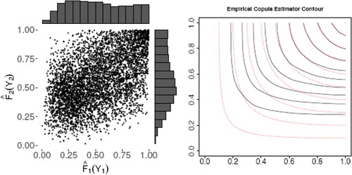
For mixed outcomes, however, the empirical copula estimator (5) is not consistent. For illustration, we include a simulated example of bivariate Tweedie outcomes whose underlying distribution and simulation procedure is described in online Appendix A. The left panel of Figure 1 displays the scatterplot of the bivariate Cox–Snell residuals. The Cox–Snell residuals of the zero-inflated mixed data are not uniformly distributed, which is reflected in the marginal histograms. In the right panel of Figure 1, the contours of the resultant empirical copula estimator (solid line) and the underlying copula (dashed line) are far apart. For this reason, the empirical copula estimator should not be directly applied to mixed data in particular when there is a significant proportion of zeros.

Fig. 1 Left: Scatterplot and marginal histograms of the bivariate Cox–Snell residuals for simulated bivariate Tweedie data. Right: Contour plot of the empirical copula estimator (solid lines) compared with the underlying copula (dashed lines).

We further analyze the probability integral transform, which is a building block for copulas. For a mixed variable Y_j , since $F_j(Y_j|X_j)⩾p_j(X_j)$ by (2), the distribution function of $F_j(Y_j|X_j)$ at $s\in (0,1)$ is(6) $$\begin{array}{c}\mathrm{Pr}(F_j(Y_j|X_j)⩽s)\hfill \\ =\{\begin{array}{cc}0\hfill & p_j(X_j)>s\hfill \\ \mathrm{Pr}(Y_j=0|X_j)\hfill & \hfill \\ +\mathrm{Pr}\left(0<Y_j⩽G_j^{-1}\left(\frac{s-p_j(X_j)}{1-p_j(X_j)}|X_j\right)|X_j\right)\hfill & p_j(X_j)⩽s\hfill \end{array}\hfill \\ =\{\begin{array}{cc}0\hfill & p_j(X_j)>s\hfill \\ p_j(X_j)+\left[1-p_j(X_j)\right]\hfill & \hfill \\ \times G_j(G_j^{-1}\left(\frac{s-p_j(X_j)}{1-p_j(X_j)}|X_j\right)|X_j)\hfill & p_j(X_j)⩽s\hfill \end{array}\hfill \\ =\{\begin{array}{cc}0\hfill & p_j(X_j)>s\hfill \\ s\hfill & p_j(X_j)⩽s.\hfill \end{array}\hfill \end{array}$$(6)

That is, if $p_j(X_j)>s$, the equation $\mathrm{Pr}(F_j(Y_j|X_j)⩽s)=s$ does not hold. Combing the two cases in (6), the probability integral transform of the mixed variable Y_j is not uniformly distributed overall. Consequently, the joint distribution function of $(F_1(Y_1|X_1),F_2(Y_2|X_2))$ in (4) is not a copula, whose marginal distributions are uniform by definition. The empirical version of (4), the empirical copula estimator (5), is therefore biased as a copula estimator for mixed data.

Extending (6) to bivariate cases, a similar argument yields that if $p_1(X_1)>s$ or $p_2(X_2)>t,\mathrm{Pr}(F_1(Y_1|X_1)⩽s,F_2(Y_2|X_2)⩽t)=0$. Only when $p_1(X_1)⩽s$ and $p_2(X_2)⩽t$, we have(7) $$\begin{array}{cc}\hfill & \hspace{1em}\mathrm{Pr}\left(F_1(Y_1|X_1)⩽s,F_2(Y_2|X_2)⩽t|p_1(X_1)⩽s,p_2(X_2)⩽t\right)\hfill \\ \hfill & =\mathrm{Pr}(Y_1⩽G_1^{-1}\left(\frac{s-p_1(X_1)}{1-p_1(X_1)}|X_1\right),\hfill \\ \hfill & \hspace{1em}{Y}_2⩽G_2^{-1}\left(\frac{t-p_2(X_2)}{1-p_2(X_2)}|X_2\right)|p_1(X_1)⩽s,p_2(X_2)⩽t)\hfill \\ \hfill & =C\{p_1(X_1)+\left[1-p_1(X_1)\right]\hfill \\ \hfill & \hspace{1em}\times G_1\left(G_1^{-1}\left(\frac{s-p_1(X_1)}{1-p_1(X_1)}|X_1\right)|X_1\right),\hfill \\ \hfill & \mathrm{\hspace{1em}}\mathrm{\hspace{1em}}{p}_2(X_2)+\left[1-p_2(X_2)\right]\hfill \\ \hfill & \hspace{1em}\times G_2(G_2^{-1}\left(\frac{t-p_2(X_2)}{1-p_2(X_2)}|X_2\right)|X_2)\}\hfill \\ \hfill & = C(s,t).\hfill \end{array}$$(7)

We aim to develop a consistent nonparametric copula estimator for multivariate mixed data. Suppose we have a sample $(X_i^{\prime },Y_{i1},Y_{i2}),i=1,\dots ,n$. When X_i varies across observations, the probabilities of zero claim $(p_1(X_{i1}),p_2(X_{i2}))$ change correspondingly. Motivated by (7), when estimating the copula at a fixed point (s, t), we focus on the subset of the observations for which $p_1(X_{i1})⩽s,p_2(X_{i2})⩽t$ holds, instead of using all the observations as is done in (5). Following the idea, we propose the “partial” empirical copula estimator$$\widehat{C}(s,t)=\frac{\sum _{i=1}^{n}1\left(F_1(Y_{i1}|X_{i1})⩽s,F_2(Y_{i2}|X_{i2})⩽t\right)}{\sum _{i=1}^{n}1\left(p_1(X_{i1})⩽s,p_2(X_{i2})⩽t\right)}.$$

In practice, the underlying marginal distributions $F_j,j=1,2$ are unknown. We adopt the inference for margin procedure (Joe 2014) to obtain the marginal coefficients estimates $\widehat{\beta }$ first. When the parameters are set to be $\widehat{\beta }$, denote the resulting marginal distribution function in (2) as $F_j(·|X_j,\widehat{\beta })$ and the probability of zero as $p_j(X_j,\widehat{\beta })$. Then one can obtain the partial empirical copula estimator(8) $$\widehat{C}(s,t;\widehat{\beta })=\frac{\sum _{i=1}^{n}1\left(F_1(Y_{i1}|X_{i1},\widehat{\beta })⩽s,F_2(Y_{i2}|X_{i2},\widehat{\beta })⩽t\right)}{\sum _{i=1}^{n}1\left(p_1(X_{i1},\widehat{\beta })⩽s,p_2(X_{i2},\widehat{\beta })⩽t\right)}.$$(8)

The implementation of (8) is straightforward.

2.4 Asymptotic Results

We first show the weak convergence of the proposed nonparametric copula estimator when the underlying parameters in the marginal models, denoted as β₀, are known. Then we analyze the copula estimator when a $\sqrt{n}$-consistent estimator of β₀ is plugged in, as in (8).

Denote the distribution function of $(p_1(X_1),p_2(X_2))$, the underlying probabilities of zero, as $p_0(s,t)=\mathrm{Pr}(p_1(X_1)⩽s,p_2(X_2)⩽t)$, which depends on the distribution of X. Let $V=(m_1,1)\times (m_2,1)$ be a subset of ${(0,1)}^2$ such that for $(s,t)\in V,p_0(s,t)$ is bounded away from zero.

Theorem 2.1.

When β₀ is known, the process $\sqrt{n}(\widehat{C}-C)$ converges to a centered Gaussian process in $l^{\infty }(V)$, with covariance function$$\frac{C(s\wedge s\prime ,t\wedge t\prime )p_0\left(s\wedge s\prime ,t\wedge t\prime \right)}{p_0(s,t)p_0(s\prime ,t\prime )}-C(s,t)C(s\prime ,t\prime ),$$

where $s\wedge s\prime =\min (s,s\prime )$.

The proofs of the theoretical results can be found in online Appendix B. Next, we show the asymptotics when a $\sqrt{n}$-consistent estimator of β₀, denoted as $\widehat{\beta }$, is plugged in. Using $P=P_{{\beta }_0}$ as the underlying distribution, we denote $Pf=\int f\mathrm{d}P$ for a given measurable function f.

Assumption 2.1. $\widehat{\beta }$ is asymptotically efficient. That is,$$n^{1/2}(\widehat{\beta }-{\beta }_0)\to N(0,{[I({\beta }_0)]}^{-1}),$$where $I(\beta )$ is the Fisher information matrix $P({\dot{l}}_{\beta }{\dot{l}}_{\beta }^{\prime })$. Moreover, $l_{\beta }(x,y_1,y_2)$ is the log-likelihood of the marginal models, and ${\dot{l}}_{\beta }(x,y_1,y_2)=\partial l_{\beta }(x,y_1,y_2)/\partial \beta$ is the score function.

The maximum likelihood estimator of GLMs satisfies the asymptotic efficiency assumption under regularity conditions. This assumption can nevertheless be relaxed to asymptotic linearity. When the parameters are set to be β, we denote $F_j(·|X_j,\beta ),p_j(X_j,\beta )$, and $G_j(·|X_j,\beta )$ as the resulting marginal distribution function, the probability of zero claim, and the distribution function of the severity, respectively. The distribution of the probabilities of zero is then $p_0(s,t;\beta )=\mathrm{Pr}(p_1(X_1,\beta )⩽s,p_2(X_2,\beta )⩽t)$. The following two assumptions are made to guarantee that the densities of $(F_1(Y_1|X_1,\beta ),F_2(Y_2|X_2,\beta ))$ and $(p_1(X_1,\beta ),p_2(X_2,\beta ))$ are bounded.

Assumption 2.2. The underlying copula C has a bounded density c on V. Its first-order partial derivatives C₁ and C₂ are continuous.

Assumption 2.3. For j = 1, 2, $F_j(y_j|x_j,\beta )$ and $F_j^{\prime }(y_j|x_j,\beta )$ are continuous functions of y_j for $y_j>0$, where $F_j^{\prime }(y_j|x_j,\beta )=\partial F_j(y_j|x_j,\beta )/\partial y_j$. The distribution of the probabilities of zero $p_0(s,t;\beta )$ has bounded second-order derivatives and continuous first-order partial derivatives with respect to (s, t).

Assumption 2.4 (Lipschitz condition). There exists a constant α₁ such that for $\beta ,\beta \prime \in B$,$$\begin{array}{c}\left|p_j(x_j,\beta )-p_j(x_j,\beta \prime )\right|⩽{\alpha }_1\left|\beta -\beta \prime \right|,\\ \left|F_j(y_j|x_j,\beta )-F_j(y_j|x_j,\beta \prime )\right|⩽{\alpha }_1\left|\beta -\beta \prime \right|,\end{array}$$where B is the space of Euclidean marginal model parameters.

A necessary condition for Assumption 2.4 is that the range of X is bounded. For notational convenience, denote the function(9) $$g_{s,t,\beta }(x,y_1,y_2)=1\left(F_1(y_1|x_1,\beta )⩽s,F_2(y_2|x_2,\beta )⩽t\right).$$(9)

Assumption 2.5.

$P{g}_{s,t,\beta }$ is differentiable with respect to β for $\beta \in B$, and the derivatives are bounded.

A necessary condition for Assumption 2.5 is that $p_j(x_j,\beta )$ and quantile functions $G_j^{-1}(s|x_j,\beta )$ and $F_j^{-1}(s|x_j,\beta )$ are differentiable with respect to β.

Theorem 2.2.

Under Assumptions 2.1–2.5, the process $\sqrt{n}(\widehat{C}(·;\widehat{\beta })-C)$ converges weakly in $l^{\infty }(V)$ to the centered process$$\frac{1}{p_0(s,t)}\mathbb{G}{f}_{s,t},(s,t)\in V$$

for $\mathbb{G}$ a standard Brownian bridge process and $f_{s,t}$ defined as$$\begin{array}{c}{f}_{s,t}(x,y_1,y_2)=g_{s,t,{\beta }_0}(x,y_1,y_2)\\ \hspace{1em}+{\left[I({\beta }_0)\right]}^{-1}{\frac{\partial P{g}_{s,t,\beta }}{\partial \beta }|}_{\beta ={\beta }_0}{\dot{l}}_{{\beta }_0}(x,y_1,y_2).\end{array}$$

The representation of the limiting process has two parts. The first part has exactly the same form as the Gaussian process in Theorem 2.1. The second part comes from the “drift” sequence $\sqrt{n}P(g_{s,t,\widehat{\beta }}-g_{s,t,{\beta }_0}).$ The partial derivatives under the Tweedie and frequency-severity marginal models are provided in the supplementary materials.

The proposed copula estimator converges uniformly to the underlying copula in the area V in which $p_0(s,t)$ is bounded away from zero. This is consistent with established theoretical results on copula identifiability. Sklar (1959) showed that the uniqueness of copulas is guaranteed in the Cartesian product of the ranges of marginal distribution functions. For the mixed type of data, the range of the marginal distribution function is $[p_j,1],j=1,2,$ in the iid case, and hence the copula is unique in $[p_1,1]\times [p_2,1]$. Under regression, $p_j(X_j)$ varies with the covariates. As we assume the copula does not change with covariates, the range for copula identifiability widens to V. As a consequence, the copula can be identified more easily if $p_1(X_1)$ and $p_2(X_2)$ are distributed around small values or spread out, whereas it can only be identified in a small region if $p_1(X_1)$ and $p_2(X_2)$ concentrate on large values. Numerical evidence of this will be presented in Section 3.

3 Simulation

In this section, we investigate the performance of the proposed partial empirical copula estimator via simulated examples. The aim of the simulation is to evaluate its finite sample estimation properties under varying underlying copula types, levels of dependence strength, and proportions of zeros.

We consider 2000 policyholders, similar to the LGPIF data, and each policyholder has two types of insurance coverage j = 1, 2. The probability of making no claim is based on the function$$p_j(X_j)={\text{logit}}^{-1}\left({\beta }_{j0}+{\beta }_{j1}{X}_{j1}+{\beta }_{j2}{X}_{j2}\right).$$

For the claim severities, we employ GB2 distributions (3). The location parameter of the GB2 distribution is further assumed as a linear combination of covariates, that is, ${\mu }_{Sj}={\beta }_{j3}+{\beta }_{j4}{X}_{j2}+{\beta }_{j5}{X}_{j3},j=1,2.$ We set $X_{j1}$ to be a dummy variable with probability of one as 0.7, $X_{j2}\sim N(0,1)$, and $X_{j3}$ is a dummy variable with probability of one as 0.4. The covariates $X_{j1},X_{j2}$, and $X_{j3}$ are independent. In this example, the covariates of the frequency and severity parts overlap. Our proposed copula estimator has no inherent restriction to covariates, and is applicable to other settings of marginal models such as Tweedie GLMs.

To explore the effects of tail dependence, we employ a Gumbel copula (with upper tail dependence), a Frank copula (no tail dependence), and a Clayton copula (with lower tail dependence) as the underlying copula. The Kendall’s tau is varied from 0.5 (low dependence) to 0.75 (high dependence). Although not reported here, similar results were obtained with other underlying copulas and dependence levels.

Meanwhile, we explore the effects of the probabilities of zero. We focus on three scenarios by controlling the value of ${\beta }_{j0},j=1,2$.

• Many zeros, ${\beta }_{j0}=2,{\beta }_{j1}=-1,{\beta }_{j2}=-2,{\beta }_{j3}=5,{\beta }_{j4}=1,{\beta }_{j5}=-1.$ On average 70% data are zeros.

• Moderate zeros, ${\beta }_{j0}=0,{\beta }_{j1}=-1,{\beta }_{j2}=-2,{\beta }_{j3}=5,{\beta }_{j4}=1,{\beta }_{j5}=-1$. On average 40% data are zeros.

• Few zeros, ${\beta }_{j0}=-2,{\beta }_{j1}=-1,{\beta }_{j2}=-2,{\beta }_{j3}=5,{\beta }_{j4}=1,{\beta }_{j5}=-1$. On average 16% data are zeros.

For each experiment, the number of replications is taken to be 500. We evaluate the performance of the estimator via the mean integrated squared error (MISE).

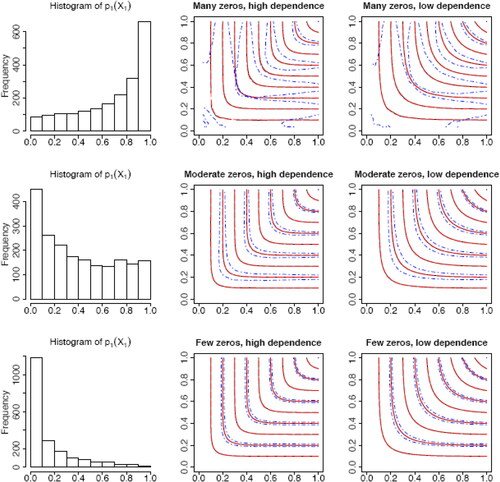
The results under Frank copulas are summarized graphically in Figure 2, which contains the histogram of the probabilities of zero in one randomly selected replication (left panel) and the contour plots of the proposed copula estimator (middle and right panels). The unbiasedness of the proposed copula estimator is apparent in the figure. In all the settings, the mean of the nonparametric copula estimator (solid lines) is very close to the underlying copula (dashed lines). The top row corresponds to the many zeros scenario. One striking impression from the contour plots in the first row is that the variance of the copula estimator tends to be large in the lower left corner. We see from the histogram that $p_1(X_1)$ is mostly distributed in the area greater than 0.5. Note that the distribution of $p_2(X_2)$ is same as $p_1(X_1)$. Consequently, $p_0(s,t)$ is small in the lower left corner and thus relatively few observations in this area satisfy $p_1(X_{i1})⩽s,p_2(X_{i2})⩽t$ to contribute to the copula estimator, causing a large variance. This is consistent with Theorem 2.2. As the proportion of zeros reduces, in the middle and bottom rows, the variance is clearly smaller. Comparing across the middle and right columns, the dependence level does not seem to have an influential effect on the performance of the nonparametric copula estimator. The graphical results for Gumbel and Clayton copulas are included in online Appendix A as Figures A1 and A2, from which one can draw consistent conclusions overall.

Fig. 2 Histogram of $p_1(X_1)$ (left column) and contour plots of the proposed copula estimator (middle and right columns). The mean of the estimator over 500 replications is given by the black solid lines, while the blue dash-dot symbols give the corresponding 95% confidence intervals, and the red dashed lines give the underlying copulas.

Table 1 presents the MISE values of the nonparametric copula estimator in different scenarios. The integration is calculated over $(0.1,1)\times (0.1,1)$, as a subset of V. Results summarized in Table 1 confirm the important influence of the proportion of zeros on the performance of the nonparametric copula estimator. When there are many zeros in the data, the estimator has a large MISE value. It is worth noting that in the many zeros scenario, the estimator has a bigger MISE value under Clayton copulas which exhibit lower tail dependence, compared to Gumbel copulas with upper tail dependence. Meanwhile, the MISE is slightly bigger under high dependence than under low dependence. With moderate zeros, the behavior of the estimator is comparable across different underlying copula families and strengths of dependence. With few zeros, the MISE value appears to be higher with low dependence.

Table 1 MISE (multiplied by 10⁴).

	Many zeros		Moderate zeros		Few zeros
	High depend	Low depend	High depend	Low depend	High depend	Low depend
Frank	13.081	11.873	1.164	1.159	0.305	0.340
Clayton	13.489	13.054	1.187	1.200	0.313	0.334
Gumbel	13.123	11.665	1.152	1.151	0.312	0.348

Our nonparametric copula estimator is applicable to higher dimensions. The copula estimator (8) can be easily extended$$\begin{array}{c}\widehat{C}(s_1,\dots ,s_d;\widehat{\beta })\\ =\frac{\sum _{i=1}^{n}1\left(F_1(Y_{i1}|X_{i1},\widehat{\beta })⩽s_1,\dots ,F_d(Y_{id}|X_{id},\widehat{\beta })⩽s_d\right)}{\sum _{i=1}^{n}1\left(p_1(X_{i1},\widehat{\beta })⩽s_1,\dots ,p_d(X_{id},\widehat{\beta })⩽s_d\right)}.\end{array}$$

We carry out a numerical experiment to assess the performance of the proposed copula estimator in three dimensions. Table 2 includes the MISE values. Due to the comparable behavior, here we only report the results under a Frank copula. With moderate and few zeros, the MISE of the estimator in three dimensions is comparable to the MISE values in the bivariate case. However, with many zeros, the MISE values in three dimensions double the results of the bivariate case. It implies that the curse of dimensionality is an issue when the proportion of zeros is high in the data.

Table 2 MISE in three dimensions (multiplied by 10⁴).

Many zeros		Moderate zeros		Few zeros
High	Low	High	Low	High	Low
depend	depend	depend	depend	depend	depend
22.383	20.866	1.890	1.760	0.320	0.351

4 Data Analysis

We apply the proposed nonparametric copula estimator to a dataset from the LGPIF. The LGPIF was established by the state of Wisconsin to provide property insurance for local government entities, and it offers different types of coverage. For example, a county entity may need motor vehicle coverage for its snow plowing trucks, in addition to building and contents coverage for its buildings. In our study, we focus on the joint modeling of claims arising from the building and contents (BC) coverage and the motor vehicle (MV) coverage.

4.1 Data Summary

Table 3 summarizes the distribution of the claims for each coverage. There are 5660 policies with coverage in BC and 2175 polices with MV coverage. Jointly, there are 2170 policies with both coverages, and we use this subset of data for dependence modeling. There are significant proportions of zeros for both coverages, around 70%. We also provide the quantiles of the severities, from which we can clearly see the right skewness and long tails of the severity distributions. This motivates the usage of long-tailed distributions such as GB2 to model the claim severities.

Table 3 Sample size, proportion of zeros, and quantiles of severities for each coverage.

	n	Zero%	5%	25%	50%	75%	95%	Max
BC	5660	0.702	1010	3380	9184	27,310	142,637	12,922,218
MV	2175	0.695	822	2414	6356	20,342	74,138	308,758
Joint	2170

Table 4 includes potential rating variables and their summary statistics. One rating variable is the entity type indicating whether the covered buildings or motor vehicles belong to a city, county, etc. In addition, the fund offers credits for fire alarms. For instance, a policyholder receives a 5% discount in premium if automatic smoke alarms are installed in some of the main rooms within the building, a 10% discount if alarms are installed in all of the main rooms, and a 15% discount if the alarms are installed and monitored in all the main rooms. We also use the coverage amounts as covariates in our analysis.

Table 4 Description and summary statistics of covariates.

Variable	Description	Mean
TypeCity	=1 if entity type is city	0.140
TypeCounty	=1 if entity type is county	0.058
TypeSchool	=1 if entity type is school	0.282
TypeTown	=1 if entity type is town	0.173
TypeVillage	=1 if entity type is village	0.237
TypeMisc	=1 if entity type is other	0.110
AC00	=1 if no alarm credit	0.466
AC05	=1 if 5% alarm credit	0.042
AC10	=1 if 10% alarm credit	0.058
AC15	=1 if 15% alarm credit	0.435
lnCoverageBC	Coverage of BC line in logarithmic millions of dollars	2.119
		(2.000)
lnCoverageMV	Coverage of MV line in logarithmic millions of dollars	–0.798
		(1.626)

4.2 Marginal Models

Since the severities are heavily skewed and long-tailed, we employ the frequency-severity approach to characterize the marginal distributions. For the frequency part, we model the probability of zero claim using logistic regression. We model the severity part using a GB2 distribution, as described in Section 2.1. The coefficients of the marginal models are included in Table 5. County entities have the smallest probability of making no claim for both BC and MV coverages. Entities belonging in the miscellaneous category have the largest severities on average. Alarm credit is a less important rating variable. Intuitively, policies with large coverages, or equivalently large risk exposures, are more likely to have positive claims and more severe claims given occurrence. The results confirm that our severity data are long-tailed, since the second moments of the fitted GB2 distributions do not exist, reflected in the fact that ${\kappa }_2<2\sigma$ for both margins.

Table 5 Marginal coefficients.

	Frequency		Severity
BC	Estimate	SE	Estimate	SE
Intercept	1.894	0.086	7.330	0.141
TypeCity	–0.226	0.107	–0.202	0.108
TypeCounty	–0.909	0.158	–0.111	0.130
TypeMisc	0.850	0.147	0.303	0.166
TypeSchool	0.730	0.103	–0.156	0.110
TypeTown	0.675	0.147	0.248	0.175
AC05	–0.288	0.164	0.172	0.177
AC10	–0.281	0.144	–0.245	0.152
AC15	–0.259	0.082	–0.100	0.086
lnCoverageBC	–0.456	0.032	0.544	0.034
σ			0.810	0.111
κ1			1.202	0.251
κ2			0.967	0.195
MV	Estimate	SE	Estimate	SE
Intercept	0.790	0.131	8.475	0.217
TypeCity	–0.170	0.201	–0.263	0.176
TypeCounty	–1.834	0.226	0.658	0.157
TypeMisc	0.892	0.401	0.704	0.427
TypeSchool	–0.414	0.162	0.262	0.161
TypeTown	1.307	0.269	0.237	0.305
lnCoverageMV	–0.728	0.054	0.514	0.049
σ			0.636	0.152
κ1			0.821	0.252
κ2			1.009	0.384

4.3 Copula Estimation and Selection

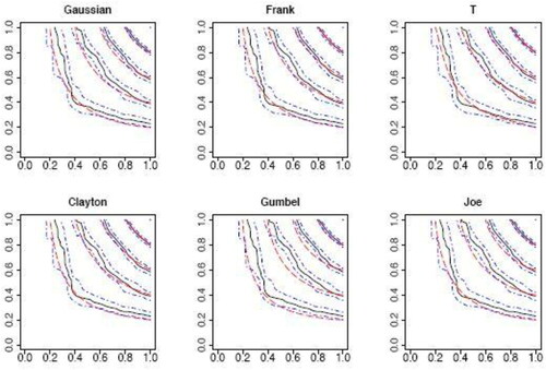
Having fit the marginal models, we then analyze the dependence structure between claims from the two types of insurance coverage using the proposed nonparametric copula estimator. The nonparametric estimator is shown in Figure 3 as the solid curves. Its confidence intervals based on 1000 bootstrap replications are displayed as the dash-dot curves. Due to the large proportion of zeros, the estimator is not smooth especially in the lower left corner, as there are sparse observations in this area.

Fig. 3 Contour plot of the nonparametric copula estimator (black solid lines) and its 90% confidence interval (blue dash-dot symbols) constructed from bootstrap, compared with fitted parametric copulas (red dashed lines).

We now demonstrate copula model selection for mixed data using our nonparametric copula estimator. We fit a set of commonly used parametric copulas through MLE. Then we compare the fitted parametric copulas with our nonparametric estimator. Table 6 includes the parameter estimates for the parametric copulas. To compare different copulas, we also convert the copula parameters into Kendall’s τ. It attracts our attention that the values of Kendall’s τ vary significantly from copula to copula, even though they are estimated from the same dataset. For continuous outcomes, in contrast, the Kendall’s τ of the fitted parametric copulas based on the analytical definition should all be close to the one of the data based on the probabilistic definition.

Table 6 Parameter estimates of parametric copulas.

	Estimate	SE	Kendall’s τ
$t(\text{df}=3)$	0.075	0.036	0.048
Gaussian	0.132	0.033	0.084
Frank	0.841	0.204	0.093
Clayton	0.291	0.070	0.127
Gumbel	1.309	0.044	0.236
Joe	1.295	0.054	0.143

Figure 3 presents the contour plots of the fitted parametric copulas (dashed lines). We see a relatively large discrepancy between the Gumbel copula and the nonparametric estimator, although in general it is hard to make definitive conclusions based on visual inspection. Hence, we quantify the discrepancy between a parametric copula and the nonparametric estimator using the L₂-norm distance(10) $$d(\widehat{C}(·;\widehat{\beta }),{\tilde{C}}_{\widehat{\gamma }})={\left\{\int (\widehat{C}(s,t;\widehat{\beta })-{\tilde{C}}_{\widehat{\gamma }}(s,t){)}^2\mathrm{d}s\mathrm{d}t\right\}}^{1/2},$$(10) where $\widehat{C}(·;\widehat{\beta })$ is the proposed nonparametric estimator, and ${\tilde{C}}_{\widehat{\gamma }}$ is the fitted parametric copula. Table 7 presents the distances. Here, we compute the integration over the range $(0.2,1)\times (0.2,1)$ to exclude the areas with sparse data. The standard deviations of the distances are obtained through bootstrap. The t copula is seen to outperform other copulas with smallest distance, followed by the Gaussian and Frank copulas. The Gumbel and Joe copulas, both with upper tail dependence, do not seem to fit the data well. We conclude, therefore, that the claims from the two types of insurance coverage have a symmetric dependence structure. The fact that the t copula is better than the Gaussian and Frank copulas suggests tail dependence in the claims. Nonetheless, tail dependence is less important than the symmetry, as copulas with asymmetric tail dependence (e.g., Clayton, Gumbel, and Joe copulas) do not provide satisfactory fitting.

Table 7 Distances $d(\widehat{C}(·;\widehat{\beta }),{\tilde{C}}_{\widehat{\gamma }})$ of different parametric copulas (multiplied by 100).

	Gaussian	Frank	t	Clayton	Gumbel	Joe
Est.	2.735	2.804	2.377	3.088	4.221	3.293
SD	0.518	0.554	0.457	0.594	0.828	0.679

5 Conclusions

This article studied the modeling of multivariate insurance claim data using copulas. Insurance claim data typically follow a mixed distribution with a point mass at zero corresponding to the case of no claim and a distribution for positive values describing the claim amount given occurrence. Our contribution is the introduction of a nonparametric copula estimator, which provides the foundation for copula identification with mixed data. We showed the weak convergence of the proposed nonparametric copula estimator. The simulation study indicated that the proportion of zeros plays an important role in copula identification for mixed data. In particular, it is difficult to identify the underlying dependence structure if the probabilities of zero concentrate on large values. We illustrated the usage of our estimator with a case study on the LGPIF data from the state of Wisconsin. The proposed nonparametric copula estimator revealed that the dependence structure between the claims from the building coverage and the motor vehicle coverage is symmetric.

Although we focused on insurance applications, the proposed methodology is applicable to other fields with similar mixed data structures. For instance, in climate research, it can be adopted to study the correlation among precipitation (e.g., rainfall) in multiple regions.

Finally, some improvements can be made on the proposed method. First, we can smooth the estimator by applying kernel smoothing methods and introducing tuning parameters. Second, we used the L₂-norm distance to quantify the discrepancy between fitted parametric copulas with our nonparametric estimator for model selection. Future work could involve studying the asymptotic properties of this distance so as to provide formal goodness-of-fit tests for copulas with mixed data. The uniform convergence results in this article have provided the essential foundation for developing goodness-of-fit tests.

Acknowledgments

The author is grateful to the reviewers for insightful comments leading to an improved article.

Supplementary Materials

The supplementary materials include a description of a simulated example of bivariate Tweedie outcomes, proofs, and additional derivations of the theoretical results.

References

- Chen, S. X., and Huang, T.-M. (2007), “Nonparametric Estimation of Copula Functions for Dependence Modelling,” Canadian Journal of Statistics, 35, 265–282. DOI: https://doi.org/10.1002/cjs.5550350205.
- Cox, D. R., and Snell, E. J. (1968), “A General Definition of Residuals,” Journal of the Royal Statistical Society, Series B, 30, 248–265. DOI: https://doi.org/10.1111/j.2517-6161.1968.tb00724.x.
- Deheuvels, P. (1979), “La fonction de Dépendance Empirique et ses Propriétés. Un Test Non paramétrique d’Indépendance,” Académie Royale de Belgique. Bulletin de la Classe des Sciences (5), 65, 274–292. DOI: https://doi.org/10.3406/barb.1979.58521.
- Frees, E. W. (2014), “Frequency and Severity Models,” in Predictive Modeling Applications in Actuarial Science, International Series on Actuarial Science (Vol. 1), Cambridge: Cambridge University Press, pp. 138–164.
- Frees, E. W., Lee, G., and Yang, L. (2016), “Multivariate Frequency-Severity Regression Models in Insurance,” Risks, 4, 4. DOI: https://doi.org/10.3390/risks4010004.
- Frees, E. W., and Valdez, E. A. (1998), “Understanding Relationships Using Copulas,” North American Actuarial Journal, 2, 1–25. DOI: https://doi.org/10.1080/10920277.1998.10595667.
- Frees, E. W., and Valdez, E. A. (2008), “Hierarchical Insurance Claims Modeling,” Journal of the American Statistical Association, 103, 1457–1469.
- Genest, C., Gerber, H. U., Goovaerts, M. J., and Laeven, R. J. A. (2009), “Modeling and Measurement of Multivariate Risk in Insurance and Finance,” Insurance: Mathematics & Economics, 44, 143–145.
- Genest, C., Rémillard, B., and Beaudoin, D. (2009), “Goodness-of-Fit Tests for Copulas: A Review and a Power Study,” Insurance: Mathematics and economics, 44, 199–213. DOI: https://doi.org/10.1016/j.insmatheco.2007.10.005.
- Gschlößl, S., and Czado, C. (2007), “Spatial Modelling of Claim Frequency and Claim Size in Non-Life Insurance,” Scandinavian Actuarial Journal, 2007, 202–225. DOI: https://doi.org/10.1080/03461230701414764.
- Joe, H. (2014), Dependence Modeling With Copulas, Boca Raton, FL: CRC Press.
- Kosorok, M. R. (2008), Introduction to Empirical Processes and Semiparametric Inference, New York: Springer-Verlag.
- McDonald, J. B., and Xu, Y. J. (1995), “A Generalization of the Beta Distribution With Applications,” Journal of Econometrics, 66, 133–152. DOI: https://doi.org/10.1016/0304-4076(94)01612-4.
- Ohlsson, E., and Johansson, B. (2006), “Exact Credibility and Tweedie Models,” Astin Bulletin, 36, 121–133. DOI: https://doi.org/10.1017/S0515036100014422.
- Omelka, M., Gijbels, I., and Veraverbeke, N. (2009), “Improved Kernel Estimation of Copulas: Weak Convergence and Goodness-of-Fit Testing,” The Annals of Statistics, 37, 3023–3058. DOI: https://doi.org/10.1214/08-AOS666.
- Shi, P. (2016), “Insurance Ratemaking Using a Copula-Based Multivariate Tweedie Model,” Scandinavian Actuarial Journal, 2016, 198–215. DOI: https://doi.org/10.1080/03461238.2014.921639.
- Shi, P., and Yang, L. (2018), “Pair Copula Constructions for Insurance Experience Rating,” Journal of the American Statistical Association, 113, 122–133. DOI: https://doi.org/10.1080/01621459.2017.1330692.
- Sklar, M (1959), “Fonctions de Répartition À N Dimensions et Leurs Marges,” Publications de l’Institut Statistique de l’Université de Paris, 8, 229–231.
- Song, P. X.-K., Li, M., and Yuan, Y. (2009), “Joint Regression Analysis of Correlated Data Using Gaussian Copulas,” Biometrics, 65, 60–68. DOI: https://doi.org/10.1111/j.1541-0420.2008.01058.x.
- van der Vaart, A. W., and Wellner, J. A. (1996), Weak Convergence and Empirical Processes With Applications to Statistics, New York: Springer.
- van der Vaart, A. W., and Wellner, J. A. (2007), “Empirical Processes Indexed by Estimated Functions,” in Asymptotics: Particles, Processes and Inverse Problems, Beachwood, OH: Institute of Mathematical Statistics, pp. 234–252.
- Yang, L., Frees, E. W., and Zhang, Z. (2020), “Nonparametric Estimation of Copula Regression Models With Discrete Outcomes,” Journal of the American Statistical Association, 115, 707–720. DOI: https://doi.org/10.1080/01621459.2018.1546586.
- Yang, L., and Shi, P. (2019), “Multiperil Rate Making for Property Insurance Using Longitudinal Data,” Journal of the Royal Statistical Society, Series A, 182, 647–668. DOI: https://doi.org/10.1111/rssa.12419.
- Zilko, A. A., and Kurowicka, D. (2016), “Copula in a Multivariate Mixed Discrete–Continuous Model,” Computational Statistics & Data Analysis, 103, 28–55.