Estimating Monotone Concave Stochastic Production Frontiers

Abstract

Recent research shows that the search for Bayesian estimation of concave production functions is a fruitful area of investigation. In this article, we use a flexible cost function that satisfies globally the monotonicity and curvature properties to estimate features of the production function. Specification of a globally monotone concave production function is a difficult task which is avoided here by using the first-order conditions for cost minimization from a globally monotone concave cost function. The problem of unavailable factor prices is bypassed by assuming structure for relative prices in the first-order conditions. The new technique is shown to perform well in a Monte Carlo experiment as well as in an empirical application to rice farming in India.

KEYWORDS:

• Bayesian analysis
• Optimization
• Productivity and competitiveness
• Stochastic frontiers

1 Introduction

Recent research shows that the search for Bayesian estimation of concave production functions is a fruitful area of investigation. This is currently a large area, started with the work of van den Broeck et al. (1994) and including Koop, Steel, and Osiewalski (1995, 1997) for the introduction of Gibbs samplers in these models, Fernandez, Osiewalski, and Steel (1997) for conditions of posterior existence under improper priors and Kumbhakar and Tsionas (2016) for endogeneity in the presence of undesirable outputs, to name but a few. Moreover, the problem of exogenous, environmental, or contextual variables that may affect inefficiency is taken up in Kumbhakar, Ghosh, and McGuckin (1991).

Arreola et al. (2020), henceforth AJCM,

use Bayesian methods and focus on relaxing standard parametric assumptions in the Stochastic Frontier Analysis (SFA) literature regarding the inefficiency and noise distributions and focus on the tradeoff between very general models of both the unobserved inefficiency and the production function.

Moreover, to model inefficiency, they extend the multivariate Bayesian convex regression (MBCR) of Hannah and Dunson (2011), to an MBCR-based semiparametric SFA method.

Additionally, Hannah and Dunson (2013) and Hannah and Dunson (2011) proposed two regression-based multivariate nonparametric convex regression methods: Least-square-based convex adaptive partitioning (CAP), and a Bayesian method, called MBCR; both scale well in large data. Using a random collection of hyperplanes, MBCR approximates a general convex multivariate regression function. Kuosmanen (2008) proposed the least-square estimator subject to concavity/convexity and monotonicity constraints, which is known as convex nonparametric least square (CNLS); see also Kuosmanen and Johnson (2010) and Kuosmanen and Kortelainen (2012). Kumbhakar et al. (2007) proposed a locally linear nonparametric approach to the estimation of efficiency where monotonicity and convexity can be imposed easily.

Moreover,

MBCR’s other attractive features include the block nature of its parameter updating, which causes parameter estimate autocorrelation to drop to zero in tens of iterations in the most cases, the ability to span all convex multivariate functions without need for any acceptance-rejection samplers, scalability to a few thousand observations, and relaxation of the homoscedastic noise assumption. Unlike CAP, the Markov Chain Monte Carlo nature of MBCR (Hannah and Dunson 2011) […]) allows modular extensions of the method without risking its convergence guarantees. Thus, we use MBCR as the basis for our estimation algorithm and focus on modeling inefficiency flexibly.

In this article, our approach to monotonization and convexification is different as we rely on functional forms that are globally monotone and concave to begin with. Such functional forms, however, have to be flexible. For example, under simple parametric restrictions, a Cobb–Douglas production function is globally monotone and concave, yet it fails to be flexible in the Diewert (1974) sense, see also Diewert and Wales (1987).¹

A standard exercise in microeconomics is to derive the production technology corresponding to the cost function $C(w,y)=A{w}_1^{\alpha }{w}_2^{1-\alpha }{y}^{\beta }$ ($A>0,0<\alpha <1,\beta >0$) (where $w_1,w_2>0$ are input prices and y > 0 is output) and show that it is, in fact, Cobb–Douglas. For more general technologies, for example, the translog, this is not analytically possible. The problem of recovering properties of the technology from the cost function is not trivial as it has been shown before by Karagiannis, Kumbhakar, and Tsionas (2004) and Kumbhakar and Wang (2006a,b). In this article, instead of attacking the problem of approximating a monotone concave production function as in AJCM, we focus on a monotone concave approximation to the cost function. This approach has a significant advantage; namely that input endogeneity can be handled easily whereas this is more difficult in AJCM who pointed out the problem but did not provide a solution.

Moreover, another advantage of starting from the cost function is that flexible production functions that respect globally monotonicity and concavity are hard to come by. This is not so for cost functions. The model is presented in Section 2. We present the semi-nonparametric extension in Section 4, after having described the production function monotone concave approximation in Section 3, in the panel of cross-sectional data. context. Monte Carlo simulation evidence is presented in Section 5 and an empirical application to rice farming in India in Section 6.

Relative to AJCM our approach is different in several respects:

1. We do not start from a production but with a globally flexible, globally concave and monotone cost function. In turn, we obtain the production function which is a nontrivial task given that the production function is self-dual only in very few cases (e.g., the Cobb–Douglas and, certainly, not for any flexible functional form).

2. AJCM do not account for endogeneity of inputs which is an important problem in modern production function estimation². In our approach, endogeneity is taken into account via the first-order conditions of profit maximization, allowing for optimization errors.

3. We do not make use of hyperplanes which are central in AJCM, stochastic nonparametric envelopment of data (StoNED) and constrained nonparametric least squares (CNLS); see Kuosmanen and Johnson (2010), and Kuosmanen and Kortelainen (2012). For another Baysian solution to the CNLS see Tsionas and Izzeldin (2018). Here, we follow different principles compared to both AJCM and Tsionas and Izzeldin (2018).

4. Our benchmark cost function (known as SFLEX) can be easily converted to a semi-parametric functional form via the method of sieves. We expect that semi-parametric formulations will behave better compared to the piecewise linear formulations of AJCM, StoNED, and CNLS.

5. We compare our model to more classical stochastic frontiers (e.g., half-normal, truncated normal, and gamma distributions for inefficiency) via predictive Bayes factors (PBF).

6. Our method of selecting a globally monotone concave cost function (and its extension via a method of sieves) is a nontrivial extension of AJCM which we use here only as a recent benchmark for motivation and comparison. From the cost function, we recover numerically the production function which has automatically all neoclassical properties (e.g., globally monotone concave. Recovering the production function from the cost function is a difficult problem but we do not have to worry about these properties as in AJCM, StoNED, and CNLS as the properties are imposed on a cost function, rather than a production function. Moreover, we never estimate a cost function but rather the production function and the associated system of equations and first-order conditions for cost minimization profit maximization (allowing for optimization and other measurement errors).

7. One does not have to solve for the production function itself, but rather estimate the parameters in the first-order conditions. This is important as the endogeneity problem is solved automatically unlike previous approaches like StoNED, CNLS and AJCM. Of course, the production function can be directly derived by numerical means if it is desired.

8. As the first-order conditions depend on prices which are, more often than not, unavailable, we treat prices as unknown.

Finally, we will compare the new techniques with StoNED and CNLS. Regarding StoNED, this relies on Kuosmanen (2008) who studied a nonparametric least-square regression that estimates endogenously the functional form of the regression from the family of continuous, monotone increasing and globally concave functions. The functions are non-differentiable. He showed that this family of functions can be characterized by a subset of continuous, piecewise linear functions whose firm-specific intercept and slope coefficients are constrained to satisfy monotonicity and concavity. His approach is called StoNED. CNLS is concerned with the shape-restricted least-square problem, which can be employed to estimate a concave (or convex) regression function (Kuosmanen and Kortelainen 2012; Keshvari and Kuosmanen 2013).

2 Model

Lewbel (1989) proposed a globally monotone and concave functional form that is also flexible. Lewbel’s (1989) functional form is called symmetric flexible (SFLEX) cost function and is given as follows:(1) $$\begin{array}{c}C(w,y)=\frac{1}{2}\sum _k\sum _{i\ne k}\sum _{j\ne k}{\gamma }_{ij}{w}_i{w}_j{w}_k^{-1}y+\sum {\beta }_{iy}{w}_{i}y\hfill \\ +\sum _i{\beta }_i{w}_i+\left(\sum _i{\beta }_i{w}_i\right)\left(1+{\beta }_y{y}^2\right),\hfill \end{array}$$(1) where $w=[w_1,\dots ,w_K]\prime \in {\mathbb{R}}_{+}^K$ denotes the vector of input prices, $y\in {\mathbb{R}}_{+}$ is output, $C:{\mathbb{R}}_{+}^K\times {\mathbb{R}}_{+}^M\to {\mathbb{R}}_{+}$ is the cost function, and ${\beta }_i,{\beta }_{iy},{\beta }_y,{\gamma }_{ij}$ are parameters subject to the symmetry constraints: ${\gamma }_{ij}={\gamma }_{ji}$. The SFLEX cost function is linearly homogeneous in all prices, treats all prices symmetrically,³ and is flexible for all prices $w\in {\mathbb{R}}_{+}^K$ except on a set of measure zero. Moreover, provided $\Gamma =[{\gamma }_{ij}]$ is negative semidefinite, the SFLEX cost function is globally concave.

The share equations are easily derived(2) $$\begin{array}{c}{s}_i=\left(\sum _{k\ne i}\sum _{j\ne k}{\gamma }_{ij}{w}_i{w}_k^{-1}\right)-\frac{1}{2}\left(\sum _{j\ne i}\sum _{k\ne i}{\gamma }_{jk}{w}_j{w}_k{w}_i^{-2}\right)\\ +{\beta }_{iy}+{\beta }_i{y}^{-1},i=1,\dots ,K.\end{array}$$(2)

Finally, the CSFLEX imposes the Cholesky decomposition $\Gamma =-A\prime A$ on SFLEX, making Γ negative semidefinite, where A is a lower triangular matrix containing unknown coefficients. Therefore, SFLEX is by definition globally concave.

As the SFLEX cost function satisfies globally the theoretical restrictions, and it is also flexible, it can be used to approximate arbitrary cost functions. However, our problem is to approximate globally production functions, especially when input prices are not available. The first-order conditions for cost minimization yield(3) $$\begin{array}{c}{\tilde{w}}_k\equiv \frac{w_k}{w_1}=\frac{\partial f(x)/\partial x_k}{\partial f(x)/\partial x_1},k=2,\dots ,K,\\ y=f(x),\end{array}$$(3) where $f:{\mathbb{R}}_{+}^K\to {\mathbb{R}}_{+}$ is the production function. In principle, this system yields input demands ${\widehat{x}}_k={\widehat{x}}_k(\tilde{w},y),k=1,\dots ,K$, where $\tilde{w}=[w_2/w_1,\dots ,w_K/w_1]\prime$. In turn, the system can be inverted to yield(4) $$y=f(x)=f\left(\widehat{x}(\tilde{w},y)\right),$$(4) where $\widehat{x}(\tilde{w},y)=[{\widehat{x}}_1(\tilde{w},y),\dots ,{\widehat{x}}_K(\tilde{w},y)]\prime$.

For given $\tilde{w}$, Equation (4)(4) $$y=f(x)=f\left(\widehat{x}(\tilde{w},y)\right),$$(4) yields y as a function of x, for given factor relative prices $\tilde{w}$. To put it differently, given $\tilde{w}$, (3) can be solved, numerically, to yield point-wise values of f(x). Such systems have been solved before, in a different context, by Karagiannis, Kumbhakar, and Tsionas (2004). The approach has been also used in Kumbhakar and Wang (2006a,b) in the case of the translog production function. The point of this article is that we do not have to solve for the production function; instead we can use Equation (9)(9) $$y=f\left(\vartheta \widehat{x}(\tilde{w},y)\right),$$(9) as is.

Regarding technical inefficiency, the cost minimization problem is(5) $$\begin{array}{c}{C}_{\vartheta }(w,y)={\min }_{x\in {\mathbb{R}}_{+}^K}w\prime x,\\ \text{subjectto};y=f(\vartheta x),\end{array}$$(5) where $\vartheta \le 1$ represents factor-saving inefficiency. But this is equivalent to(6) $$\begin{array}{c}{C}_{\vartheta }(w,y)={\vartheta }^{-1}{\min }_{x\in {\mathbb{R}}_{+}^K}w\prime X,\\ \text{subjectto};y=f(X),\end{array}$$(6) where $X=\vartheta x$ and, therefore, $C_{\vartheta }(w,y)={\vartheta }^{-1}C(w,y)$. In log terms, this yields the familiar expression(7) $$\text{log}\hspace{0.17em}{C}_{\vartheta }(w,y)=\hspace{0.17em}\text{log}\hspace{0.17em}{C}_{\vartheta }(w,y)+u,$$(7) where $u=-\hspace{0.17em}\text{log}\hspace{0.17em}\vartheta \ge 0$ represents cost inefficiency. Therefore, the first-order conditions in Equation (4)(4) $$y=f(x)=f\left(\widehat{x}(\tilde{w},y)\right),$$(4) become(8) $$\begin{array}{c}{\tilde{w}}_k\equiv \frac{w_k}{w_1}=\frac{\partial f(x)/\partial x_k}{\partial f(x)/\partial x_1},k=2,\dots ,K,\\ y=f(\vartheta x),\end{array}$$(8) and the implicit Equation (4)(4) $$y=f(x)=f\left(\widehat{x}(\tilde{w},y)\right),$$(4) becomes(9) $$y=f\left(\vartheta \widehat{x}(\tilde{w},y)\right),$$(9) where $\widehat{x}(\tilde{w},y)=[{\widehat{x}}_1(\tilde{w},y),\dots ,{\widehat{x}}_K(\tilde{w},y)]\prime$. In general, y is a nonlinear function of ϑ.

An important additional problem is that factor relative prices are often not available, and (9) requires nonlinear solution techniques. Let us now suppose that we have cross-sectional data. This the case examined in AJCM. We take up the case of panel data in the next section.

Since from SFLEX, we have the optimal shares$${\widehat{s}}_k(\tilde{w},y)=\frac{w_k{\widehat{x}}_k(\tilde{w},y)}{\sum _{j=1}^K{w}_j{\widehat{x}}_j(\tilde{w},y)},$$we also have:(10) $${\widehat{x}}_k(\tilde{w},y)=\frac{{\widehat{s}}_k(w,y)}{p_k}\sum _{j=1}^K{w}_j{\widehat{x}}_j(\tilde{w},y),;k=1,\dots ,K.$$(10)

This technique can automatically take account of input endogeneity as there are enough equations to model these quantities. However, to recover the production function, we also need(11) $$y=f(\vartheta \widehat{x}(\tilde{w},y)).$$(11)

Other than the (self-dual) Cobb–Douglas and CES production functions, solving Equations (10)(10) $${\widehat{x}}_k(\tilde{w},y)=\frac{{\widehat{s}}_k(w,y)}{p_k}\sum _{j=1}^K{w}_j{\widehat{x}}_j(\tilde{w},y),;k=1,\dots ,K.$$(10) and (11)(11) $$y=f(\vartheta \widehat{x}(\tilde{w},y)).$$(11) requires numerical solution techniques. The minimal requirement is that we have observed data, say $\mathcal{Y}={\{y_i,x_i\}}_{i=1}^n$. It is reasonable to assume that(12) $$x_{ki}={\widehat{x}}_k(w_{ki},y_i)+v_{2,k,i},;k=1,\dots ,K,;i=1,\dots ,n,$$(12) where $v_{k,i}$ represents measurement or allocative errors. Additionally, we have the production function(13) $$y_i=f({\vartheta }_i{x}_i)+v_{i,1},$$(13) where $v_{i,1}$ is measurement error. We also assume firm-specific ${\vartheta }_i$s. In the vector form, we have(14) $$\begin{array}{c}{y}_i=f({\vartheta }_i{x}_i)+v_{i,1},\\ {\mathbf{x}}_i=\widehat{\mathbf{x}}({\tilde{w}}_i,y_i)+{\mathbf{v}}_{i,2},i=1,\dots ,n,\end{array}$$(14) where ${\mathbf{v}}_{i,2}$ is a K-dimensional error vector. That is, input endogeneity is explicitly accounted for, through the additional first-order conditions of cost minimization. Of course, we have only K equations for the K endogenous variables (input quantities) because in cost minimization output is taken as given.

Although we have treated output as exogenous, an assumption compatible with cost minimization, this can rarely satisfied in practice and, certainly, beats the purpose of estimating production functions. Output can be made endogenous via the formulation in the first equation of (14).

To examine profit maximization, we use the familiar condition that output price is equal to marginal cost(15) $$\begin{array}{c}{p}_i=\frac{\partial C(w_i,y_i){\vartheta }_i^{-1}}{\partial y_i}\Rightarrow \hspace{0.17em}\text{log}\hspace{0.17em}\frac{\partial \hspace{0.17em}\text{log}\hspace{0.17em}C(w_i,y_i)}{\partial \hspace{0.17em}\text{log}\hspace{0.17em}{y}_i}\\ =\hspace{0.17em}\text{log}\hspace{0.17em}{y}_i+\hspace{0.17em}\text{log}\hspace{0.17em}{p}_i-\hspace{0.17em}\text{log}\hspace{0.17em}C(w_i,y_i).\end{array}$$(15)

If we add an error term ($v_{i,3}$) to take account of market imperfections and/or deviations from profit maximizing behavior, then we have(16) $$\text{log}\hspace{0.17em}{e}_{cy,i}-\hspace{0.17em}\text{log}\hspace{0.17em}{y}_i-\hspace{0.17em}\text{log}\hspace{0.17em}{p}_i+\hspace{0.17em}\text{log}\hspace{0.17em}C(w_i,y_i)-\hspace{0.17em}\text{log}\hspace{0.17em}{\vartheta }_i=v_{i,3},$$(16) where $e_{cy,i}\equiv \frac{\partial \hspace{0.17em}\text{log}\hspace{0.17em}C(w_i,y_i)}{\partial \hspace{0.17em}\text{log}\hspace{0.17em}{y}_i}$. This provides the additional equation needed to endogenize output y_i although (i) it appears in a nonlinear way, and (ii) product prices are unavailable.

To summarize, we have the following system of equations:(17) $$\begin{array}{c}{y}_i=f({\vartheta }_i{x}_i)+v_{i,1},\\ x_i=\widehat{x}({\tilde{w}}_i,y_i)+{\mathbf{v}}_{i,2},i=1,\dots ,n,\\ \hspace{0.17em}\text{log}\hspace{0.17em}{e}_{cy,i}-\hspace{0.17em}\text{log}\hspace{0.17em}{y}_i-\hspace{0.17em}\text{log}\hspace{0.17em}{p}_i+\hspace{0.17em}\text{log}\hspace{0.17em}C(w_i,y_i)-\hspace{0.17em}\text{log}\hspace{0.17em}{\vartheta }_i=v_{i,4},\\ {\mathbf{V}}_i=[v_{i,1},{\mathbf{v}}_{i,2}^{\prime },v_{i,3},v_{i,4}]\prime \sim {\mathcal{N}}_{K+3}(\mathbf{0},\mathbf{\Sigma }),i=1,\dots ,n.\end{array}$$(17)

To proceed, in the presence of unavailable factor relative prices and product price, we have to make assumptions about them. In cross-sectional data, there is not much choice, and one assumption is that prices are common for all units. Clearly, this is an assumption that cannot be defended in practice although its advantage is that we only introduce K + 1 additional parameters (input relative prices and output price).

The most reasonable assumption is to relate prices to certain predetermined variables ${\mathit{z}}_i\in {\mathbb{R}}^m$ (18) $$\begin{array}{c}\hspace{0.17em}\text{log}\hspace{0.17em}{\tilde{w}}_i=({\mathbf{I}}_{K-1}\otimes \mathit{z}{\prime }_i){\delta }_1+{\mathbf{e}}_{i,1},\\ \hspace{0.17em}\text{log}\hspace{0.17em}{p}_i=\mathit{z}{\prime }_i{\delta }_2+e_{i,2},\\ {\mathbf{e}}_i=[{\mathbf{e}}_{i,1},e_{i,2}]\prime \sim {\mathcal{N}}_K(\mathbf{0},\Omega ),\\ i=1,\dots ,n,\end{array}$$(18) where ${\mathit{z}}_i\in {\mathbb{R}}^m$ is a vector of environmental variables that can be related to relative prices and product price. We assume ${\mathit{z}}_i$ includes at least a column of ones, and ${\delta }_1=[\delta {\prime }_1,;\delta {\prime }_2,;\dots ;\delta {\prime }_K]\prime \in {\mathbb{R}}^{mK},{\delta }_K\in {\mathbb{R}}^m$, contain unknown parameters.

We can combine the first two equations to have(19) $$\text{log}\hspace{0.17em}\widetilde{{\varpi }_i}:=\left[\begin{array}{c}\hspace{0.17em}\text{log}\hspace{0.17em}{\tilde{w}}_i\\ \hspace{0.17em}\text{log}\hspace{0.17em}{p}_i\end{array}\right]=({\mathbf{I}}_K\otimes \mathit{z}{\prime }_i)\delta +{\mathbf{e}}_i,;i=1,\dots ,n,$$(19) where $\delta =[\delta {\prime }_1,{\delta }_2]\prime \in {\mathbb{R}}^{mK}$, and we use the symbol $\text{log}\hspace{0.17em}\widetilde{{\varpi }_i}$ to denote from now on, log relative factor prices and the log of product price.

To see the first equation clearly, we have(20) $$\begin{array}{c}\hspace{0.17em}\text{log}\hspace{0.17em}{\tilde{\varpi }}_{i,1}=\mathit{z}{\prime }_i{\delta }_1+e_{i,1},\\ \hspace{0.17em}\text{log}\hspace{0.17em}{\tilde{\varpi }}_{i,2}=\mathit{z}{\prime }_i{\delta }_2+e_{i,2},\\ ⋮\\ \hspace{0.17em}\text{log}\hspace{0.17em}{\tilde{\varpi }}_{i,K}=\mathit{z}{\prime }_i{\delta }_K+e_{i,K},\end{array}$$(20)

As noted in AJCM, their “primary contribution is the first single-stage method that allows a shaped-constrained production frontier to be estimated nonparametrically, relaxes the homoscedastic assumption on the inefficiency term, and estimates the impact of environmental variables for the analysis of cross sectional data.” Our own contribution is that we can incorporate additional information from (imperfect) profit maximization with unknown input and output prices.

To introduce heteroscedasticity and environmental variables in the context of cross-sectional data, we assume(21) $$\begin{array}{c}\hspace{0.17em}\text{log}\hspace{0.17em}{u}_i|{\mathit{z}}_i\sim \mathcal{N}(\mathit{z}{\prime }_i{\mathit{\gamma }}_1,;{\sigma }_{u,i}^2),;i=1,\dots ,n,\\ \hspace{0.17em}\text{log}\hspace{0.17em}{\sigma }_{u,i}^2=\mathit{z}{\prime }_i{\mathit{\gamma }}_2,;i=1,\dots ,n,\end{array}$$(21) where $u_i\ge 0$ represents inefficiency (see Equation (7)(7) $$\text{log}\hspace{0.17em}{C}_{\vartheta }(w,y)=\hspace{0.17em}\text{log}\hspace{0.17em}{C}_{\vartheta }(w,y)+u,$$(7) ), ${\mathit{\gamma }}_1,{\mathit{\gamma }}_2\in {\mathbb{R}}^m$ are vectors of unknown parameters. We assume that the environmental variables used to model relative prices and product price in (18) on the one hand, and inefficiency on the other are the same, although this assumption is made purely to simplify notation.

As alternatives to Equation (21)(21) $$\begin{array}{c}\hspace{0.17em}\text{log}\hspace{0.17em}{u}_i|{\mathit{z}}_i\sim \mathcal{N}(\mathit{z}{\prime }_i{\mathit{\gamma }}_1,;{\sigma }_{u,i}^2),;i=1,\dots ,n,\\ \hspace{0.17em}\text{log}\hspace{0.17em}{\sigma }_{u,i}^2=\mathit{z}{\prime }_i{\mathit{\gamma }}_2,;i=1,\dots ,n,\end{array}$$(21) we propose, for purposes of robustness the following competing models:(22) $$u_i|{\mathit{z}}_i\sim {\mathcal{N}}_{+}\left(\mathit{z}{\prime }_i{\mathit{\gamma }}_1,;e^{\mathit{z}{\prime }_i{\mathit{\gamma }}_2}\right),\text{Truncated Normal}(\text{TN})\text{model}$$(22) (23) $$\begin{array}{c}p(u_i|{\mathit{z}}_i)=\frac{{\lambda }^p}{{\mu }^p(p-1)!}{x}^{p-1}{e}^{-x/\mu },\\ p=1,2,3,\text{Erlang}-\mathit{gamma}(\text{EG})\text{model},\end{array}$$(23) (24) $$\text{log}\hspace{0.17em}{\mu }_i=z{\prime }_i{\mathit{\gamma }}_1.$$(24)

For the Erlang distributions, see van den Broeck et al. (1994) who were the first to use it. Notice that the mean of EG is $p{\mu }_i$ and the variance is $p{\mu }_i^2$ so the model is always heteroscedastic. The TN model assumes a truncated normal distribution for inefficiency with location $\mathit{z}{\prime }_i{\mathit{\gamma }}_1$ and scale $e^{\mathit{z}{\prime }_i{\mathit{\gamma }}_2}$. For ${\mathit{\gamma }}_1=0$ we obtain the half-normal (HN) distribution with observation-specification variance. If ${\mathit{z}}_i$ includes only a constant term then we have the homoscedastic HN model and the homoscedastic EG model with constant mean and variance.

The EG model assumes a gamma distribution for inefficiency, with integer values of the shape parameter (p) using p = 1, 2, 3. For p = 1, we obtain an exponential distribution and p = 2 corresponds to chi-squared. For values higher than p = 3, the distribution looks like the normal distribution so identification would be tenuous.

3 The Model With Panel Data

Although in this article, we focus on cross-sectional data, we provide a few details on how panel data may be used. In the case of panel data, the major problem is that the K prices ${\tilde{\varpi }}_{it}$ are, again, unknown. As we have panel data, a reasonable assumption in the absence of such data is(25) $$\text{log}\hspace{0.17em}{\tilde{\varpi }}_{it}={\mathit{\mu }}_i+{\mathit{\lambda }}_t+{\mathit{\xi }}_{it},$$(25) where ${\mathit{\mu }}_i$ and ${\mathit{\lambda }}_t$ are K-dimensional firm and time effects, and ξ_it is a K-dimensional error term. One possibility is to assume random effects, viz. ${\mathit{\mu }}_i\sim {\mathcal{N}}_K(\mathbf{0},{\sigma }_{\mu }^2{\mathbf{I}}_K)$ ($i=1,\dots ,n$), ${\mathit{\lambda }}_t\sim {\mathcal{N}}_K(\mathbf{0},{\sigma }_{\lambda }^2{\mathbf{I}}_{K-1})$ ($t=1,\dots ,T$), and(26) $${\mathit{\xi }}_{it}\sim {\mathcal{N}}_K(\mathbf{0},{\sigma }_{\xi }^2{\mathbf{I}}_K),i=1,\dots ,n,t=1,\dots ,T.$$(26)

The last assumption is reasonable. The other two assumptions are not, since firm and time effects may be correlated with the inputs. In this work, we follow the Chamberlain (1982, 1984) and Mundlak (1978) approach in making the firm the time effects functions of the x_its, thus obtaining a range a intermediate situations between purely random and purely fixed effects. The presence of the error term ${\mathit{\xi }}_{it}$ allows for random effects and the following assumptions allow for fixed effects:(27) $$\underset{K\times 1}{{\mathit{\mu }}_i}=\sum _{t=1}^T\underset{K\times K}{{\mathbf{\Psi }}_t}{x}_{it},i=1,\dots ,n,$$(27) (28) $$\underset{K\times 1}{{\lambda }_t}=\sum _{i=1}^n\underset{K\times K}{{\mathbf{\Phi }}_i}{x}_{it},t=1,\dots ,T,$$(28) where the matrices ${\mathbf{\Psi }}_t$ and ${\mathbf{\Phi }}_i$ contain unknown coefficients. In total they contain $d\equiv (n+T)K(K-1)$ unknown coefficients. As this can be exceedingly large, we use a “regularization” prior of the form:(29) $$\mathit{\psi }\equiv \text{vec}[{\left\{{\mathbf{\Psi }}_t\right\}}_{t=1}^T,{\left\{{\mathbf{\Phi }}_i\right\}}_{i=1}^n]\sim {\mathcal{N}}_d(\overline{\psi }{\mathbf{1}}_d,{\overline{\sigma }}_{\psi }^2{\mathbf{I}}_d),$$(29) where ${\mathbf{1}}_d$ denotes a vector of ones in ${\mathbb{R}}^d$, and $\text{vec}(·)$ is the vectorization operator that stacks rows of a matrix into a vector. We treat $\overline{\psi }=0$, and ${\overline{\sigma }}_{\psi }=1$ as fixed parameters which, however, we will vary when we will perform sensitivity analysis with respect to the prior.

Our final system consists of Equations (17)(17) $$\begin{array}{c}{y}_i=f({\vartheta }_i{x}_i)+v_{i,1},\\ x_i=\widehat{x}({\tilde{w}}_i,y_i)+{\mathbf{v}}_{i,2},i=1,\dots ,n,\\ \hspace{0.17em}\text{log}\hspace{0.17em}{e}_{cy,i}-\hspace{0.17em}\text{log}\hspace{0.17em}{y}_i-\hspace{0.17em}\text{log}\hspace{0.17em}{p}_i+\hspace{0.17em}\text{log}\hspace{0.17em}C(w_i,y_i)-\hspace{0.17em}\text{log}\hspace{0.17em}{\vartheta }_i=v_{i,4},\\ {\mathbf{V}}_i=[v_{i,1},{\mathbf{v}}_{i,2}^{\prime },v_{i,3},v_{i,4}]\prime \sim {\mathcal{N}}_{K+3}(\mathbf{0},\mathbf{\Sigma }),i=1,\dots ,n.\end{array}$$(17) , (14)(14) $$\begin{array}{c}{y}_i=f({\vartheta }_i{x}_i)+v_{i,1},\\ {\mathbf{x}}_i=\widehat{\mathbf{x}}({\tilde{w}}_i,y_i)+{\mathbf{v}}_{i,2},i=1,\dots ,n,\end{array}$$(14) , the distributional assumption on the system errors’ normality, and the effects assumptions in Equations (26)–(28). In line with much of the literature we also assume Equation (21)(21) $$\begin{array}{c}\hspace{0.17em}\text{log}\hspace{0.17em}{u}_i|{\mathit{z}}_i\sim \mathcal{N}(\mathit{z}{\prime }_i{\mathit{\gamma }}_1,;{\sigma }_{u,i}^2),;i=1,\dots ,n,\\ \hspace{0.17em}\text{log}\hspace{0.17em}{\sigma }_{u,i}^2=\mathit{z}{\prime }_i{\mathit{\gamma }}_2,;i=1,\dots ,n,\end{array}$$(21) is in place. The details of estimation are left for future research as our focus here is on cross-sectional data.

4 Semi-Nonparametric Extension

One can argue that SFLEX yields a flexible monotone concave frontier but it is still a parametric functional form unlike AJCM. To turn SFLEX into a semi-nonparametric formulation, we remind that $\text{log}\hspace{0.17em}\tilde{\varpi }$ contains log relative factor prices and log output price, defined in ${\mathbb{R}}^K.$ Suppose $C(\tilde{w},y;\beta )$ denotes an SFLEX cost function with parameter vector β and $\text{log}\hspace{0.17em}\tilde{\varpi }=[\text{log}\hspace{0.17em}\tilde{w},\hspace{0.17em}\text{log}\hspace{0.17em}p]\prime$. Although this formulation applies to panel data, we illustrate here the case of cross-sectional data in the interest of clarity. Given the data on ${\mathit{q}}_i={\{\hspace{0.17em}\text{log}\hspace{0.17em}{w}_i\}}_{i=1}^n$, we propose the following semi-nonparametric extension of SFLEX:(30) $$C({\check{w}}_i,y_i;\beta )=\sum _{g\in \mathbb{G}}{\tau }_{g}C({\tilde{w}}_i,y_i;{\beta }_g),;i=1,\dots ,n,$$(30) where $\mathbb{G}=\{1,\dots ,G\}$, and the weights ${\tau }_g\ge 0$ ($g\in \mathbb{G}$), $\sum _{g\in \mathbb{G}}{\tau }_g=1$. This is a normal mixture distribution and a member of the class of sieves (Gallant and Nychka 1987).⁴ Our prior on $\{{\tau }_g,g\in \mathbb{G}\}$ is uniform over the unit simplex.

As G increases it is straightforward to show that the extended semi-nonparametric SFLEX, or SNP-SFLEX can approximate even more closely any monotone concave cost function (** White 1989, 1990). Given the first-order conditions for cost minimization and the first-order condition for profit maximization, there is an associated demand system like Equations (17)(17) $$\begin{array}{c}{y}_i=f({\vartheta }_i{x}_i)+v_{i,1},\\ x_i=\widehat{x}({\tilde{w}}_i,y_i)+{\mathbf{v}}_{i,2},i=1,\dots ,n,\\ \hspace{0.17em}\text{log}\hspace{0.17em}{e}_{cy,i}-\hspace{0.17em}\text{log}\hspace{0.17em}{y}_i-\hspace{0.17em}\text{log}\hspace{0.17em}{p}_i+\hspace{0.17em}\text{log}\hspace{0.17em}C(w_i,y_i)-\hspace{0.17em}\text{log}\hspace{0.17em}{\vartheta }_i=v_{i,4},\\ {\mathbf{V}}_i=[v_{i,1},{\mathbf{v}}_{i,2}^{\prime },v_{i,3},v_{i,4}]\prime \sim {\mathcal{N}}_{K+3}(\mathbf{0},\mathbf{\Sigma }),i=1,\dots ,n.\end{array}$$(17) and (21)(21) $$\begin{array}{c}\hspace{0.17em}\text{log}\hspace{0.17em}{u}_i|{\mathit{z}}_i\sim \mathcal{N}(\mathit{z}{\prime }_i{\mathit{\gamma }}_1,;{\sigma }_{u,i}^2),;i=1,\dots ,n,\\ \hspace{0.17em}\text{log}\hspace{0.17em}{\sigma }_{u,i}^2=\mathit{z}{\prime }_i{\mathit{\gamma }}_2,;i=1,\dots ,n,\end{array}$$(21) for each $g\in \mathbb{G}$.

To determine the number of mixing components G (G > 2), we use the posterior odds ratio (also known as Bayes Factor when the prior odds is 1:1 for models corresponding to different Gs). For any model with parameters $\theta \in \Theta \subseteq {\mathfrak{R}}^d$, data $\mathit{Y}$, likelihood $\mathit{L}(\theta ;\mathit{Y})$ and prior $p(\theta )$ the marginal likelihood or evidence is defined as $\mathit{M}(\mathit{Y})=\int \mathit{L}(\theta ;\mathit{Y})p(\theta )\mathrm{d}\theta$, that is, the integrating constant of the posterior. With prior odds 1:1, the posterior odds ratio in favor of model “A” and against model “B” is given by(31) $${\text{BF}}_{A:B}=\frac{{\mathit{M}}_A(\mathit{Y})}{{\mathit{M}}_B(\mathit{Y})}=\frac{{\int }_{\Theta }{\mathit{L}}_A({\theta }_A;\mathit{Y})p({\theta }_A)\mathrm{d}{\theta }_A}{{\int }_{\Theta }{\mathit{L}}_B({\theta }_B;\mathit{Y})p({\theta }_B)\mathrm{d}{\theta }_B},$$(31) in obvious notation. Noting that the posterior is $p(\theta |\mathit{Y})=\frac{\mathit{L}(\theta ;\mathit{Y})p(\theta )}{{\int }_{\Theta }\mathit{L}(\theta ;\mathit{Y})p(\theta )\mathrm{d}\theta }=\frac{\mathit{L}(\theta ;\mathit{Y})p(\theta )}{\mathit{M}(\mathit{Y})}$, we have the following identity for marginal likelihood known as “candidate’s formula:”(32) $$\mathit{M}(\mathit{Y})=\frac{\mathit{L}(\theta ;\mathit{Y})p(\theta )}{p(\theta |\mathit{Y})},$$(32) , for all θ. As this holds for any parameter vector it holds also for the posterior mean $\overline{\theta }$: $\mathit{M}(\mathit{Y})=\frac{\mathit{L}(\overline{\theta };\mathit{Y})p(\overline{\theta })}{p(\overline{\theta }|\mathit{Y})}$. Approximating the denominator with a multivariate normal distribution, we have(33) $$\mathit{M}(\mathit{Y})=\mathit{L}(\overline{\theta };\mathit{Y})p(\overline{\theta }){(2\pi )}^{d/2}|\overline{V}{|}^{1/2},$$(33) where $\overline{V}$ is an estimate of the posterior covariance matrix of θ which we can get easily from MCMC output.

5 Monte Carlo Evidence

We use the same data-generating processes as in AJCM. Their Example 1 uses a two-factor Cobb–Douglas production function with homoscedastic inefficiency, and their Example 2 uses a thee-factor Cobb–Douglas production function with heteroscedastic inefficiency. Therefore, in Example 1, we have $y_i=f({\mathit{x}}_i)e^{v_i-u_i}=x_{i1}^{0.4}{x}_{i2}^{0.5}{e}^{v_i-u_i}$, where $v_i\sim \mathcal{N}(0,{\sigma }_v^2)$, and u_i follows an exponential distribution with mean ${\sigma }_u=\frac{1}{6}$ where the noise-to-signal ratio varies as $\rho =\frac{{\sigma }_v}{{\sigma }_u}\in \{1,2,3\}$. Moreover, $i=1,\dots ,n$ where n is the sample size. In Example 2, we have $y_i=f({\mathit{x}}_i)e^{v_i-u_i}=x_{i1}^{0.4}{x}_{i2}^{0.3}{x}_{i3}^{0.2}{e}^{v_i-u_i}$, $v_i\sim \mathcal{N}(0,{\sigma }_v^2),u_i|x_i\sim {\mathcal{N}}_{+}(0,{\sigma }_u(x_{i1}+x_{i2}))$, where ${\sigma }_u=0.3$, and ${\sigma }_v=\rho {\sigma }_u\sqrt{\frac{\pi -2}{\pi }}$.

We do not generate explicitly production function data. Instead, we use the self-dual Cobb–Douglas cost functions using $C_i=A{w}_{i1}^{\alpha }{w}_{i2}^{1-\alpha }{y}_i^{\beta }$, in the bivariate case and similarly in the trivariate case. Factor prices are generated from a standard log-normal distribution. The self-dual production function is $y_i=C{x}_{i1}^{\alpha /\beta }{x}_{i2}^{(1-\alpha )/\beta }$, where C is a constant that depends on $A,\alpha ,\beta$. To maintain the comparison with StoNED and MCBR, we modify directly the production function as $y_i=C{x}_{i1}^{\alpha /\beta }{x}_{i2}^{(1-\alpha )/\beta }{e}^{v_i-u_i}$ using the AJCM specifications for v_i and u_i.

AJCM compare their results with the StoNED approach of Kuosmanen and Kortelainen (2012), as StoNED is the only shape-constrained frontier estimation method that can handle more than a few hundred observations. The approaches are compared in terms of mean squared error for the functional form, ${\text{MSE}}_f=n^{-1}{\sum }_{i=1}^n{(f_i-{\widehat{f}}_i)}^2$, as well as quality of inefficiency estimation, defined as ${\text{MSE}}_u=n^{-1}{\sum }_{i=1}^n{({\widehat{u}}_i-\overline{u})}^2$.

6 Empirical Application

6.1 General

Annual data from 1975–1976 to 1984–1985 on farmers from the village of Aurepalle in India are used in this empirical illustration. This dataset and a subset of it have been used by Battese, and Coelli (1995) and Coelli, and Battese (1996). We have the following variables:

Y is the total value of output; Land is the total area of irrigated and nonirrigated land operated; PI Land is the proportion of operated land that is irrigated; Labor is the total hours of family and hired labor; Bullock is the hours of bullock labor; Cost is the value of other inputs, including fertilizer, manure, pesticides, machinery, etc.; D a variable which has a value of one if Cost is positive, and a value of zero if otherwise; Age is the age of the primary decision-maker in the farming operation; Schooling is the years of formal schooling of the primary decision maker; and Year is the year of the observations involved. (Wang 2002, pp. 245–246)

The data are an unbalanced panel of 34 farmers with a total of 271 observations but we treat it as a cross section. Inputs are (logs of) Land, PI Land, Labor, Bullocks, and $\text{log}\hspace{0.17em}(\max (\text{Cost}),;1-D)$ (Figure 1).

Fig. 1 Aspects of the model.

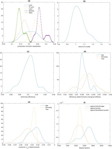
In panel (f), we report sample distributions of Bayes factor (BF) in favor of SFLEX and against the Cobb–Douglas, the translog and the Generalized Leontief. To obtain these sample distributions, we omit randomly all observations for B firms (where B is randomly selected in $\left\{10,;20,\dots ,100\right\}$), and we re-estimate the two models. This is performed 10,000 times. The BF is defined as(34) $${\text{BF}}_{12}=\frac{p(\mathit{Y}|{\mathcal{M}}_1)}{p(\mathit{Y}|{\mathcal{M}}_2)},$$(34) where $p(\mathit{Y}|{\mathcal{M}}_1)$ is the likelihood of the data (when parameter uncertainty has been taken into account) under model ${\mathcal{M}}_1$ and $p(\mathit{Y}|{\mathcal{M}}_2)$ is the probability to observe the data under model ${\mathcal{M}}_2$. Apparently, the SFLEX model is strongly favored by the data. The number of points, G, in Equation (30)(30) $$C({\check{w}}_i,y_i;\beta )=\sum _{g\in \mathbb{G}}{\tau }_{g}C({\tilde{w}}_i,y_i;{\beta }_g),;i=1,\dots ,n,$$(30) ranges from 3 to 5 with a modal value of 3 across different priors. For the benchmark prior, we find that the BF strongly supports ⁵ $G=3.$

The BFs are obtained using the procedure of Perrakis, Ntzoufras, and Tsionas (2014). Re-estimation of models is performed using sampling-importance-resampling (SIR; Rubin 1987, 1988) to avoid computationally expensive MCMC.⁶

6.2 Model Comparison

In this subsection, we take up the problem of model comparison using predictive BF (Gneiting and Raftery 2007). Given a dataset $\mathit{Y}$ we split it into an in-sample set for estimation (denoted ${\mathit{Y}}_o$) and an out-of-sample set (denoted ${\mathit{Y}}_1$ with $\mathit{Y}={\mathit{Y}}_1\cup {\mathit{Y}}_0$) which is used for computing the predictive marginal likelihood(35) $$\text{PML}=p({\mathit{Y}}_1|{\mathit{Y}}_o)=\int p(\theta ,{\mathit{Y}}_1|{\mathit{Y}}_o)\mathrm{d}\theta =$$(35) (36) $$\int p({\mathit{Y}}_1|\theta ,{\mathit{Y}}_o)p(\theta |{\mathit{Y}}_o)\mathrm{d}\theta .$$(36)

The term $p(\theta |{\mathit{Y}}_o)$ is the posterior of the parameters conditional on the in-sample observations and the multivariate integral in (36) can be accurately approximated as follows. Suppose $\left\{{\theta }^{(s)},s=1,\dots ,S\right\}$ is a sample that converges to the distribution whose density is $p(\theta |{\mathit{Y}}_o)$. In turn, the integral is approximated using(37) $$\text{PML}({\mathit{Y}}_1)=S^{-1}\sum _{s=1}^{S}p({\mathit{Y}}_1|{\theta }^{(s)},{\mathit{Y}}_o).$$(37)

With independent observations, this reduces to$$\text{PML}({\mathit{Y}}_1)=S^{-1}\sum _{s=1}^{S}p({\mathit{Y}}_1|{\theta }^{(s)}),$$which is fairly easy to compute. We denote by ${\text{PML}}_{0:j}$ the predictive marginal likelihood of our new model using Equations (21)(21) $$\begin{array}{c}\hspace{0.17em}\text{log}\hspace{0.17em}{u}_i|{\mathit{z}}_i\sim \mathcal{N}(\mathit{z}{\prime }_i{\mathit{\gamma }}_1,;{\sigma }_{u,i}^2),;i=1,\dots ,n,\\ \hspace{0.17em}\text{log}\hspace{0.17em}{\sigma }_{u,i}^2=\mathit{z}{\prime }_i{\mathit{\gamma }}_2,;i=1,\dots ,n,\end{array}$$(21) , (22)–(24) against a certain model j. The PBF are defined as(38) $${\text{PBF}}_{0:j}=\frac{{\text{PML}}_0({\mathit{Y}}_1)}{{\text{PML}}_j({\mathit{Y}}_1)},$$(38) where the “j” corresponds to Equations (21)(21) $$\begin{array}{c}\hspace{0.17em}\text{log}\hspace{0.17em}{u}_i|{\mathit{z}}_i\sim \mathcal{N}(\mathit{z}{\prime }_i{\mathit{\gamma }}_1,;{\sigma }_{u,i}^2),;i=1,\dots ,n,\\ \hspace{0.17em}\text{log}\hspace{0.17em}{\sigma }_{u,i}^2=\mathit{z}{\prime }_i{\mathit{\gamma }}_2,;i=1,\dots ,n,\end{array}$$(21) , (22)–(24). We use 75% of observations for the in-sample observations ${\mathit{Y}}_o$ and 25% in the predictive set ${\mathit{Y}}_1$. The predictive set is generated using resampling without replacement from the entire dataset $\mathit{Y}$. Marginal likelihoods are approximated using the methodology in Section 6.1. We repeat this exercise 1000 times so that we have 1000 different PBFs for each model j.

In panels (a) and (b) of Figure 2, we report distributions of PBFs in favor of the “0” model and against ten competing models for inefficiency. These distributions arise from using 1000 different samples for in- and out-of-sample observation sets.

Fig. 2 Predictive Bayes factors in favor of new model and against other formulations for inefficiency.

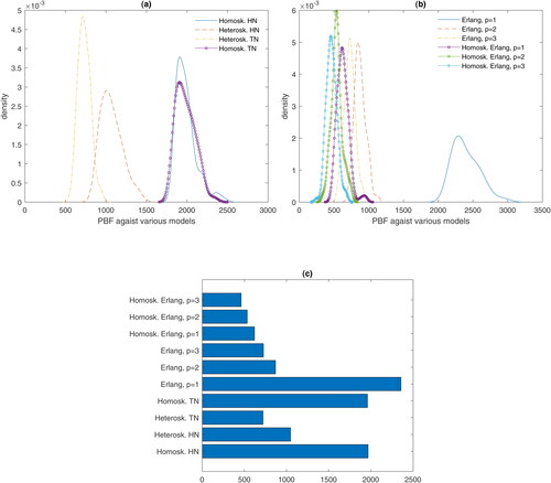
In panel (c), we present the median PBFs in favor of the new specification against 10 other alternatives as in Equations (22)–(24).

In panel (a) of Figure 3, we report efficiency distributions from different inefficiency models (the thick line corresponds to the new model). In panel (b), we report rank correlation coefficients between efficiency in the new model with all other 10 models.

Fig. 3 Efficiency distributions corresponding to different models.

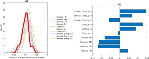
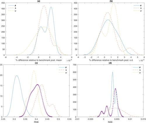
Fig. B.1 Prior sensitivity and numerical performance.

7 Concluding Remarks

The problem of constructing globally monotone concave production frontiers (especially with cross-sectional data) is a difficult one as it has been shown by AJCM. In this article, we start from a globally monotone concave flexible cost frontier and we estimate aspects of the production function without actually having to solve for the daunting task of recovering the production function from the cost function. The problem has an analytical (self-dual) solution in only two cases; the Cobb–Douglas and the CES cost functions whose production functions are also Cobb–Douglas and CES, respectively. However, these functional forms are not flexible in the precise sense put forward by Diewert (1974). We avoid nonlinear solution techniques to recover the production function from a (globally monotone concave) cost function by using the first-order conditions for cost minimization. As input prices are unobserved we assume structure for log relative prices and, in this way, we solve another major problem in estimating production functions, namely that inputs are endogenous. Input endogeneity is automatically taken into account through the additional equations provided by cost minimization.

It is possible to use the exact same procedure with a general transformation function that would allow the handling of multiple outputs.We leave the matter for future research with the hint that cost minimization is compatible with an input-oriented distance function.

Table 1 Monte Carlo results: bivariate Cobb–Douglas.

		${\text{MSE}}_f$			${\text{MSE}}_u$
ρ	n	StoNED	MCBR	This article	StoNED	MCBR	This article
	100	0.0022	0.0038	0.0019	–0.020	0.030	0.019
1	200	0.0015	0.0018	0.0013	– 0.020	0.040	0.0082
	300	0.0014	0.0016	0.0008	–0.020	0.020	0.0065
	500	0.0004	0.0012	0.0006	– 0.010	0.020	0.0057
	100	0.0058	0.0040	0.0032	0.02	0.010	0.0072
2	200	0.0051	0.0050	0.0028	0.01	0.060	0.0061
	300	0.0045	0.0036	0.0017	0.01	0.030	0.0044
	500	0.0047	0.0014	0.0012	0.07	0.00	0.0022
	100	0.0237	0.0175	0.0122	0.10	0.12	0.0034
3	200	0.0259	0.0057	0.0044	0.14	0.00	0.0012
	300	0.0306	0.0046	0.0031	0.17	–0.02	0.0004
	500	0.0270	0.0032	0.0021	0.13	–0.06	0.0002

NOTES: StoNED and MCBR (the method in AJCM) results are taken from Table 1 of AJCM. The number of points, G, in Equation (30)(30) $$C({\check{w}}_i,y_i;\beta )=\sum _{g\in \mathbb{G}}{\tau }_{g}C({\tilde{w}}_i,y_i;{\beta }_g),;i=1,\dots ,n,$$(30) ranges from 3 to 4 with a modal value of 3.

Table 2 Monte Carlo results: trivariate Cobb–Douglas.

		${\text{MSE}}_f$			${\text{MSE}}_u$
ρ	n	StoNED	MCBR	This article	StoNED	MCBR	This article
	100	0.0058	0.0071	0.0044	0.10	0.11	0.054
1	200	0.0047	0.0033	0.0040	0.10	0.07	0.050
	300	0.0047	0.0045	0.0032	0.10	0.1	0.032
	500	0.0499	0.0019	0.0012	0.33, 0.02	0.04	0.014
	100	0.0507	0.0194	0.010	0.28	0.22	0.078
2	200	0.0407	0.0126	0.0076	0.27, 0.08	0.16	0.065
	300	0.0590	0.0052	0.0043	0.33, 0.12	0.06	0.040
	500	0.1345	0.0023	0.0010	0.47, 0.05	0.03	0.012
	100	0.149	0.0205	0.0133	0.38, 0.28	0.18	0.055
3	200	0.1955	0.0068	0.0031	0.50, 0.33	0.06	0.030
	300	0.2446	0.005	0.002	0.58, 0.29	0.04	0.012
	500	0.2610	0.0038	0.002	0.63, -0.02	0.04	0.008

NOTES: StoNED and MCBR (the method in AJCM) results are taken from Table 3 of AJCM. The number of points, G, in Equation (30)(30) $$C({\check{w}}_i,y_i;\beta )=\sum _{g\in \mathbb{G}}{\tau }_{g}C({\tilde{w}}_i,y_i;{\beta }_g),;i=1,\dots ,n,$$(30) ranges from 3 to 4 with a modal value of 3.

Table 3 Empirical results.

	Post. mean	Post. median	Post. s.d.
			Production function elasticities
Land	0.206	0.209	0.033
PI land	0.171	0.172	0.021
Labor	0.241	0.239	0.023
Bullocks	0.266	0.259	0.025
Other	0.149	0.143	0.019
RTS	1.033	1.024	0.067
Efficiency	0.912	0.906	0.012
			Efficiency determinants
Age	0.037	0.036	0.004
Schooling	0.039	0.041	0.0071
Year	0.040	0.038	0.055
			$\text{log}\hspace{0.17em}{\sigma }_{\xi i}^2$ determinants
Age	−0.036	−0.034	0.008
Schooling	−0.050	−0.048	0.010
Year	−0.039	−0.037	0.006

Acknowledgments

The author wishes to thank the Editor and the anonymous reviewers for their useful comments on an earlier version.

Appendix A

We write compactly Equation (17)(17) $$\begin{array}{c}{y}_i=f({\vartheta }_i{x}_i)+v_{i,1},\\ x_i=\widehat{x}({\tilde{w}}_i,y_i)+{\mathbf{v}}_{i,2},i=1,\dots ,n,\\ \hspace{0.17em}\text{log}\hspace{0.17em}{e}_{cy,i}-\hspace{0.17em}\text{log}\hspace{0.17em}{y}_i-\hspace{0.17em}\text{log}\hspace{0.17em}{p}_i+\hspace{0.17em}\text{log}\hspace{0.17em}C(w_i,y_i)-\hspace{0.17em}\text{log}\hspace{0.17em}{\vartheta }_i=v_{i,4},\\ {\mathbf{V}}_i=[v_{i,1},{\mathbf{v}}_{i,2}^{\prime },v_{i,3},v_{i,4}]\prime \sim {\mathcal{N}}_{K+3}(\mathbf{0},\mathbf{\Sigma }),i=1,\dots ,n.\end{array}$$(17) in the following form:(A.1) $$\mathfrak{F}(y_i,x_i,{\vartheta }_i,{\tilde{w}}_i)={\mathbf{v}}_i,;v_i\sim {\mathcal{N}}_{K+1}(\mathbf{0},\mathbf{\Sigma }),;i=1,\dots ,n,$$(A.1) along with the model specifications in Equations (21)(21) $$\begin{array}{c}\hspace{0.17em}\text{log}\hspace{0.17em}{u}_i|{\mathit{z}}_i\sim \mathcal{N}(\mathit{z}{\prime }_i{\mathit{\gamma }}_1,;{\sigma }_{u,i}^2),;i=1,\dots ,n,\\ \hspace{0.17em}\text{log}\hspace{0.17em}{\sigma }_{u,i}^2=\mathit{z}{\prime }_i{\mathit{\gamma }}_2,;i=1,\dots ,n,\end{array}$$(21) , (18)(18) $$\begin{array}{c}\hspace{0.17em}\text{log}\hspace{0.17em}{\tilde{w}}_i=({\mathbf{I}}_{K-1}\otimes \mathit{z}{\prime }_i){\delta }_1+{\mathbf{e}}_{i,1},\\ \hspace{0.17em}\text{log}\hspace{0.17em}{p}_i=\mathit{z}{\prime }_i{\delta }_2+e_{i,2},\\ {\mathbf{e}}_i=[{\mathbf{e}}_{i,1},e_{i,2}]\prime \sim {\mathcal{N}}_K(\mathbf{0},\Omega ),\\ i=1,\dots ,n,\end{array}$$(18) .

The complete data likelihood (that includes observed and unobserved data) is given by(A.2) $$\begin{array}{c}\mathit{L}(\mathit{\theta },\mathbf{\Sigma },\mathbf{\Omega };\mathcal{Y},\mathcal{U})\propto \\ |\mathbf{\Sigma }{|}^{-n/2}\hspace{0.17em}\text{exp}\hspace{0.17em}\left\{-\frac{1}{2}\sum _{i=1}^n\mathfrak{F}(y_i,x_i,{\vartheta }_i,{\tilde{w}}_i)\prime {\mathbf{\Sigma }}^{-1}\mathfrak{F}(y_i,x_i,{\vartheta }_i,{\tilde{w}}_i)\right\}·\\ |\mathbf{\Omega }{|}^{-1/2}\hspace{0.17em}\text{exp}\hspace{0.17em}\left\{-\frac{1}{2}\sum _{i=1}^n(\hspace{0.17em}\text{log}\hspace{0.17em}{\tilde{w}}_i-\mathit{\mu })\prime {\mathbf{\Omega }}^{-1}(\hspace{0.17em}\text{log}\hspace{0.17em}{\tilde{w}}_i-\mathit{\mu })-\sum _{i=1}^n\hspace{0.17em}\text{log}\hspace{0.17em}{\tilde{w}}_i\right\}·\\ \hspace{0.17em}\text{exp}\hspace{0.17em}\left\{-\frac{1}{2}\sum _{i=1}^n\frac{{(\hspace{0.17em}\text{log}\hspace{0.17em}{\vartheta }_i-z_i^{\prime }{\mathit{\gamma }}_1)}^2}{{\sigma }_{\xi i}^2}-\frac{1}{2}\sum _{i=1}^n\hspace{0.17em}\text{log}\hspace{0.17em}{\sigma }_{\xi i}^2-\sum _{i=1}^n\hspace{0.17em}\text{log}\hspace{0.17em}{\vartheta }_i\right\}.\end{array}$$(A.2) where ${\sigma }_{\xi i}^2\equiv z{\prime }_i{\mathit{\gamma }}_2,\mathit{\theta }\in {\mathbb{R}}^P$ denotes all unknown parameters⁷ (P being the dimensionality of the parameter vector), $\mathcal{Y}$ contains all observed data ${\{y_i,x_i\}}_{i=1}^n$, and U contains the latent variables ${\tilde{w}}_i$ and ${\vartheta }_i$. The additional terms $-{\sum }_{i=1}^n\hspace{0.17em}\text{log}\hspace{0.17em}{\tilde{w}}_i$ and $-{\sum }_{i=1}^n\hspace{0.17em}\text{log}\hspace{0.17em}{\vartheta }_i$ come from the log-normality assumptions. Given a prior $p(\mathit{\theta })$, by Bayes’ theorem, we have the augmented posterior distribution whose density is given as(A.3) $$p(\mathit{\theta },\mathbf{\Sigma },\mathbf{\Omega },\mathcal{U}|\mathcal{Y})\propto \mathit{L}(\mathit{\theta },\mathbf{\Sigma },\mathbf{\Omega };\mathcal{Y},\mathcal{U})p(\mathit{\theta }).$$(A.3)

Our “reference prior” is(A.4) $$\begin{array}{c}\mathit{\theta }|\mathbf{\Sigma },\mathbf{\Omega }\sim {\mathcal{N}}_P(\overline{\mathit{\theta }},;{\Psi }_{\mathit{\theta }})\\ p(\mathbf{\Sigma })\propto |\mathbf{\Sigma }{|}^{-(\overline{n}+K_1+1)/2}\hspace{0.17em}\text{exp}\hspace{0.17em}\left(-\text{tr}{\overline{\mathbf{A}}}_{\mathbf{\Sigma }}{\mathbf{\Sigma }}^{-1}\right),\\ p(\mathbf{\Omega })\propto |\mathbf{\Omega }{|}^{-(\overline{n}+K_2+1)/2}\hspace{0.17em}\text{exp}\hspace{0.17em}\left(-\text{tr}{\overline{\mathbf{A}}}_{\mathbf{\Omega }}{\mathbf{\Omega }}^{-1}\right),\end{array}$$(A.4) where $K_1=K+1,K_2=K-1$ (see Zellner 1971, pp. 225, 227, eq. (8.15)) $\overline{\mathit{\theta }}$ is the prior mean, ${\Psi }_{\mathit{\theta }}$ is the prior covariance matrix, $\overline{n}\ge 0$ and ${\overline{\mathbf{A}}}_{\mathbf{\Sigma }},{\overline{\mathbf{A}}}_{\mathbf{\Omega }}$ contain parameters related to the prior. We set $\overline{\mathit{\theta }}=\mathbf{0}$, ${\Psi }_{\mathit{\theta }}={\overline{h}}^2{\mathbf{I}}_P$ (where ${\mathbf{I}}_P$ is the P × P identity matrix), $\overline{h}=10,\overline{n}=1$, and ${\overline{\mathbf{A}}}_{\mathbf{\Sigma }},{\overline{\mathbf{A}}}_{\mathbf{\Omega }}$ are diagonal matrices ($K_1\times 1$ and $K_2\times 1$, respectively) containing the scalar $\overline{a}={10}^{-3}$ along their main diagonal.

For estimation and inference, we use a Gibbs sampler that draws successively from the following posterior conditional distributions:(A.5) $$p(\mathit{\theta }|\mathbf{\Sigma },\mathbf{\Omega },{\left\{{\vartheta }_i\right\}}_{i=1}^n,{\left\{{\tilde{w}}_i\right\}}_{i=1}^n,\mathcal{Y}),$$(A.5) (A.6) $$p(\mathbf{\Sigma }|\mathit{\theta },\mathbf{\Omega },{\left\{{\vartheta }_i\right\}}_{i=1}^n,{\left\{{\tilde{w}}_i\right\}}_{i=1}^n,\mathcal{Y}),$$(A.6) (A.7) $$p(\mathbf{\Omega }|\mathit{\theta },\mathbf{\Sigma },{\left\{{\vartheta }_i\right\}}_{i=1}^n,{\left\{{\tilde{w}}_i\right\}}_{i=1}^n,\mathcal{Y}),$$(A.7) (A.8) $$p({\vartheta }_i|\mathit{\theta },\mathbf{\Sigma },\mathbf{\Omega },{\left\{{\tilde{w}}_i\right\}}_{i=1}^n,\mathcal{Y}),;i=1,\dots ,n,$$(A.8) (A.9) $$p({\tilde{w}}_i|\mathit{\theta },\mathbf{\Sigma },\mathbf{\Omega },{\left\{{\vartheta }_i\right\}}_{i=1}^n,\mathcal{Y}),;i=1,\dots ,n.$$(A.9)

Drawings from the posterior conditionals in Equations (A.6)(A.6) $$p(\mathbf{\Sigma }|\mathit{\theta },\mathbf{\Omega },{\left\{{\vartheta }_i\right\}}_{i=1}^n,{\left\{{\tilde{w}}_i\right\}}_{i=1}^n,\mathcal{Y}),$$(A.6) and (A.7) are easy to realize as they belong to the inverted Wishart family (Zellner 1971, pp. 395 and 396). If we define the typical member of this family as (the different elements of) an m × m positive definite matrix V, then we write $\mathit{V}\sim \mathcal{I}\mathcal{W}(\nu ,\mathit{A})$ when its density is(A.10) $$p(\mathit{V})\propto |\mathit{V}{|}^{-(\nu +m+1)/2}\hspace{0.17em}\text{exp}\hspace{0.17em}\left(-\frac{1}{2}\text{tr}\mathit{A}{\mathit{V}}^{-1}\right).$$(A.10)

The degrees of freedom are $\nu =n+\overline{n}$ for both $\mathbf{\Sigma }$ and $\mathbf{\Omega },m=K_1$ and $m=K_2$, respectively, and the scale matrices are, respectively, ${\mathit{A}}_{\mathbf{\Sigma }}={\overline{\mathbf{A}}}_{\mathbf{\Sigma }}+{\sum }_{i=1}^n\mathfrak{F}(y_i,x_i,{\vartheta }_i,{\tilde{w}}_i)\mathfrak{F}(y_i,x_i,{\vartheta }_i,{\tilde{w}}_i)\prime$, and ${\mathit{A}}_{\mathbf{\Omega }}={\overline{\mathbf{A}}}_{\mathbf{\Omega }}+{\sum }_{i=1}^n(\hspace{0.17em}\text{log}\hspace{0.17em}{\tilde{w}}_i-\mathit{\mu })(\hspace{0.17em}\text{log}\hspace{0.17em}{\tilde{w}}_i-\mathit{\mu })\prime$.

To draw $\mathit{\theta }$ from Equation (A.5)(A.5) $$p(\mathit{\theta }|\mathbf{\Sigma },\mathbf{\Omega },{\left\{{\vartheta }_i\right\}}_{i=1}^n,{\left\{{\tilde{w}}_i\right\}}_{i=1}^n,\mathcal{Y}),$$(A.5) , we use a random-walk type Metropolis–Hastings algorithm: Given the current draw, say ${\mathit{\theta }}^{(s)}$ (where s denotes the MCMC iteration) we draw a candidate vector ${\mathit{\theta }}^{*}\sim {\mathcal{N}}_P({\mathit{\theta }}^{(s)},;c^2{\mathbf{I}}_P)$. The draw is accepted with the Metropolis–Hastings probability $\min \left\{1,;\frac{p({\mathit{\theta }}^{*}|\mathbf{\Sigma },\mathbf{\Omega },{\left\{{\vartheta }_i\right\}}_{i=1}^n,{\left\{{\tilde{w}}_i\right\}}_{i=1}^n,\mathcal{Y}}{p({\mathit{\theta }}^{(s)}|\mathbf{\Sigma },\mathbf{\Omega },{\left\{{\vartheta }_i\right\}}_{i=1}^n,{\left\{{\tilde{w}}_i\right\}}_{i=1}^n,\mathcal{Y}}\right\}$, else we set ${\mathit{\theta }}^{(s+1)}={\mathit{\theta }}^{(s)}$ (conditioning on other parameters is at their values from the sth MCMC iteration). The constant c > 0 is calibrated during the burn-in phase so that the acceptance rate is close to 20%.

To draw from the posterior conditionals of ${\mathit{\lambda }}_i\equiv [{\vartheta }_i,{\tilde{w}}_i]\prime$ in Equations (A.8)(A.8) $$p({\vartheta }_i|\mathit{\theta },\mathbf{\Sigma },\mathbf{\Omega },{\left\{{\tilde{w}}_i\right\}}_{i=1}^n,\mathcal{Y}),;i=1,\dots ,n,$$(A.8) and (A.9), we find the mode of the joint conditional log-posterior $\text{log}\hspace{0.17em}p({\mathit{\lambda }}_i|\mathit{\theta },\mathbf{\Sigma },\mathbf{\Omega },\mathcal{Y})$ ($i=1,\dots ,n$) along with an estimate of its Hessian$${\mathit{H}}_i\equiv {\partial }^2\hspace{0.17em}\text{log}\hspace{0.17em}p({\widehat{\mathit{\lambda }}}_i|\mathit{\theta },\mathbf{\Sigma },\mathbf{\Omega },\mathcal{Y})/\partial {\mathit{\lambda }}_i\partial \mathit{\lambda }{\prime }_i,;i=1,\dots ,n,$$where ${\widehat{\mathit{\lambda }}}_i$ is the mode. Define ${\mathit{V}}_i={(-{\mathit{H}}_i)}^{-1}$. In turn, we draw a candidate ${\mathit{\lambda }}_i^{*}\sim {\mathcal{N}}_2(\widehat{{\mathit{\lambda }}_i},;c_o^2{\mathit{V}}_i)$. Suppose the bivariate normal density is denoted by $f_{\mathcal{N}}(\mathbf{x};\mathbf{m},\mathbf{V})$. Then, we accept the candidate with the Metropolis–Hastings probability $\min \left\{1,;\frac{p({\mathit{\lambda }}_i^{*}|\mathit{\theta },\mathbf{\Sigma },\mathbf{\Omega },\mathcal{Y})/f_{\mathcal{N}}({\mathit{\lambda }}_i^{*};{\widehat{\mathit{\lambda }}}_i,{\mathit{V}}_i)}{p({\mathit{\lambda }}_i^{(s)}|\mathit{\theta },\mathbf{\Sigma },\mathbf{\Omega },\mathcal{Y})/f_{\mathcal{N}}({\mathit{\lambda }}_i^{(s)};{\widehat{\mathit{\lambda }}}_i,{\mathit{V}}_i)}\right\}$ (conditioning on other parameters is at their values from the sth MCMC iteration). The constant c_o > 0 is calibrated during the burn-in phase so that the acceptance rate is close to 20%. It is important to notice that these optimizations are not expensive as we are optimizing with respect to two variables at a time (viz. $\text{log}\hspace{0.17em}{\vartheta }_i$ and $\text{log}\hspace{0.17em}{\tilde{w}}_i$). Although this is expensive when n runs in the hundreds of thousands, it suffices to take one Newton step away from the fully optimized values during the burn-in phase. Finally, we use 150,000 MCMC iterations the first 50,000 of which are used in the burn-in phase to mitigate possible start-up effects and calibrate the various constants (c_o and c, including the mode and Hessian of each log-posterior of ${\lambda }_i,i=1,\dots ,n$).

Appendix B

In this appendix, we examine the behavior of MCMC as well as sensitivity to prior assumptions. We consider 10,000 priors obtained as follows:(B.1) $$\begin{array}{c}\mathit{\theta }\sim {\mathcal{N}}_P(0,;{10}^2{\mathbf{I}}_P),\\ \overline{n}\in \{0,1,\dots ,10\},\text{discrete uniform prior},\\ \hspace{0.17em}\text{log}\hspace{0.17em}\overline{h}\sim \mathcal{N}(0,;{10}^2),\\ \overline{a}\in ({10}^{-4},;{10}^3),;\text{unifom prior}.\end{array}$$(B.1)

The model is re-estimated via SIR and percentage differences relative to posterior means corresponding to the benchmark prior are reported in Figure B.1. These differences are reported in the form of kernel densities, separately for the parameters $\mathbf{\Theta }$, the latent variables ${\mathit{\lambda }}_t$, and log relative prices ${\mathit{\omega }}_{it}$ (recall that the dimensionality of this vector is $(J-1)\times 1$). In panel (a), we report percentage differences of posterior means, and in panel (b) reported are percentage differences of posterior standard deviations. From these results, it turns out that posterior moments of parameters and latent variables are fairly robust to prior assumptions.

To assess numerical performance of MCMC, we focus on relative numerical efficiency (RNE) and MCMC autocorrelation draws for Ω_it as results were roughly the same for other latent variables and parameters. RNE is a measure of closeness to iid drawings from the posterior (A.3) and, ideally, it should be equal to one, iid sampling has been possible. We report median RNE for all MCMC draws of Ω_it ($\forall i=1,\dots ,n,;t=1,\dots ,T$) in panel (c) of Figure B.1. In panel (d) of the same figure, we report numerical standard errors (NSE, see Geweke 1992). The conclusion is that all reported results are accurate to the decimal places reported.

Notes

¹Diewert and Wales (1987) showed that the popular translog loses flexibility when global concavity is imposed as it reduces to the Cobb–Douglas functional form.

²See Ackerberg, Caves, and G. Frazer (2015), Doraszelski and Jaumandreu (2013), Gandhi, Navarro, and Rivers (2020), Levinsohn and Petrin (2003), Marschak and Andrews (1944), Olley and Pakes (1996) and Wooldridge (2009).

³This is important as, for example, the McFadden (1978) cost function is globally monotone and concave but does not treat symmetrically all input prices.

⁴ We have experimented with an alternative procedure where we proceed as follows. Under the assumption that the data are (log) normally distributed, say $\mathcal{N}(\mathit{\mu },\mathit{S})$, we can generate draws as ${\overline{\mathit{q}}}^{(g)}=\mathit{\mu }+{\mathit{S}}^{-1/2}\mathit{\zeta }$, where $\mathit{\zeta }\sim \mathcal{N}(\mathit{0},\mathbf{I})$. If there are multiple clusters in the data, then we would have different ${\mathit{\mu }}^c$ and ${\mathit{S}}^c$ for each cluster ($c=1,\dots ,C$). To examine the possibility of different clusters, we use an EM algorithm to classify the data into a maximum of five clusters but we fail to find statistically significant differences between the moments ${\mathit{\mu }}^c,{\mathit{S}}^c$. In turn, this implies that the data come from a single cluster (after taking logs). For other datasets, where the possibility of clusters is real, we recommend using a run of the EM algorithm to identify approximately the moments ${\mathit{\mu }}^c,{\mathit{S}}^c$ and generate G – 2 benchmark point around each mode. Finally, to make sure that we have explored the data space adequately, we compute, for each point, the statistic $Q=({\overline{\mathit{q}}}^{(g)}-\mathit{\mu })\prime {\mathit{S}}^{-1}({\overline{\mathit{q}}}^{(g)}-\mathit{\mu })$ which, under normality, follows the chi-squared distribution (if we treat $\mathit{\mu }$ and S as the true population parameters) with degrees of freedom equal to the dimensionality of ${\overline{\mathit{q}}}^{(g)}$ or ${\mathit{q}}_i$. In turn, we sample additional points in the tails of the dataset by including another G – 2 points in the vicinity of the 5% critical value of Q so, finally, the number of benchmark points is twice the number we report in the article. “In the vicinity of the 5% critical value of Q” means that we have at least G – 2 points whose Q statistic is between the 1% and 10% critical value of the chi-squared distribution.

⁵ The BF in favor of G = 3 against G = 4, G = 5 and G = 10 were, respectively, 247.81, 338.51, and 442.70.

⁶ For SIR we use a random sub-sample of length 10,000 from the original MCMC sample

⁷ This includes parameters of the cost function, μ, and ${\mathit{\gamma }}_1,{\mathit{\gamma }}_2.$

References

- Ackerberg, D. A., Caves, K., and Frazer, G. (2015), “Identification Properties of Recent Production Function Estimators,” Econometrica, 83, 2411–2451. DOI: https://doi.org/10.3982/ECTA13408.
- Arreola, J. L., Johnson, A. L., Chen, X., and Morita, H. (2020), “Estimating Stochastic Production Frontiers: A One-Stage Multivariate Semiparametric Bayesian Concave Regression Method,” European Journal of Operational Research, 287, 699–711. DOI: https://doi.org/10.1016/j.ejor.2020.01.029.
- Battese, G. E., and Coelli, T. J. (1995), “A Model for Technical Inefficiency Effects in a Stochastic Frontier Production Function for Panel Data,” Empirical Economics, 20, 325–332. DOI: https://doi.org/10.1007/BF01205442.
- Chamberlain, G. (1982), “Multivariate Regression Models for Panel Data,” Journal of Econometrics, 5–46. DOI: https://doi.org/10.1016/0304-4076(82)90094-X.
- Chamberlain, G. (1984), “Panel Data,” in Handbook of Econometrics (Vol. 2), eds. Z. Griliches and M. D. Intriligator. Amsterdam: North Holland, pp. 1247–1318.
- Coelli, T. J., and Battese, G. E. (1996), “Identification of Factors which Influence the Technical Inefficiency of Indian Farmers,” Australian Journal of Agricultural Economics, 40, 103–128. DOI: https://doi.org/10.1111/j.1467-8489.1996.tb00558.x.
- Diewert, W. E., 1974, “Applications of Duality Theory,” in Frontiers of Quantitative Economics (Vol. II), eds. M.D. Intriligator and D.A. Kendrick, Amsterdam: North-Holland, pp. 106–171.
- Diewert, W. E., and Wales, T. J. (1987), “Flexible Functional Forms and Global Curvature Conditions,” Econometrica, 55, 43–68. DOI: https://doi.org/10.2307/1911156.
- Doraszelski, U., and Jaumandreu, J. (2013), “R&D and Productivity: Estimating Endogenous Productivity,” Review of Economic Studies, 80, 1338–1383.
- Gallant, A. R., and Nychka, D. W. (1987), “Semi-Nonparametric Maximum Likelihood Estimation,” Econometrica, 55, 363–390. DOI: https://doi.org/10.2307/1913241.
- Gandhi, A., Navarro, S., and Rivers, D. A. (2020), “On the Identification of Gross Output Production Functions,” Journal of Political Economy, 128, 2973–3016. DOI: https://doi.org/10.1086/707736.
- Gneiting, T., and Raftery, A. (2007), “Strictly Proper Scoring Rules, Prediction and Estimation,” Journal of the American Statistical Association, 102, 359–378. DOI: https://doi.org/10.1198/016214506000001437.
- Geweke, J. (1992), “Evaluating the Accuracy of Sampling-Based Approaches to the Calculation of Posterior Moments,” in Bayesian Statistics 4, eds. J. M. Bernardo, J. Berger, A. P. Dawid, and A. F. M. Smith, Oxford, U.K.: Oxford University Press, pp. 169–193.
- Fernandez, C., Osiewalski, J., and Steel, M.F.J. (1997), “On the Use of Panel Data in Stochastic Frontier Models With Improper Priors,” Journal of Econometrics, 79, 169–193. DOI: https://doi.org/10.1016/S0304-4076(97)88050-5.
- Hannah, L. A., and Dunson, D. B., (2011), “Bayesian Nonparametric Multivariate Convex Regression,” arXiv: 1109.0322.
- Hannah, L. A., and Dunson, D. B. (2013), “Multivariate Convex Regression With Adaptive Partitioning,” The Journal of Machine Learning Research, 14, 3261–3294.
- Karagiannis, G., Kumbhakar, S. C., and Tsionas, M. G. (2004), “A Distance Function Approach for Estimating Technical and Allocative Inefficiency,” Indian Economic Review, 39, 19–30.
- Keshvari, A., and Kuosmanen, T. (2013), “Stochastic Non-Convex Envelopment of Data: Applying Isotonic Regression to Frontier Estimation,” European Journal of Operational Research, 231, 481–491 DOI: https://doi.org/10.1016/j.ejor.2013.06.005.
- Koop G., Osiewalski J., and Steel M. F. J. (1997), “Bayesian Efficiency Analysis Through Individual Effects: Hospital Cost Frontiers,” Journal of Econometrics, 76, 77–105. DOI: https://doi.org/10.1016/0304-4076(95)01783-6.
- Kumbhakar, S. C., Ghosh, S., and McGuckin, J. T. (1991), “A Generalized Production Frontier Approach for Estimating Determinants of Inefficiency in U.S. Dairy Farms,” Journal of Business and Economic Statistics, 9, 279–286.
- Koop G., Steel M. F. J., and Osiewalski J. (1995), “Posterior Analysis of Stochastic Frontiers Models Using Gibbs Sampling,” Computational Statistics, 10, 353–373.
- Kumbhakar, S. C., Park, B. U., Simar, L., and Tsionas, E. G. (2007), “Nonparametric Stochastic Frontiers: A Local Maximum Likelihood Approach,” Journal of Econometrics, 137, 1–27. DOI: https://doi.org/10.1016/j.jeconom.2006.03.006.
- Kumbhakar, S. C., and Tsionas, E. G. (2016), “The Good, the Bad and the Technology: Endogeneity in Environmental Production Models,” Journal of Econometrics, 190, 315–327 DOI: https://doi.org/10.1016/j.jeconom.2015.06.008.
- Kumbhakar, S. C., and Wang, H-Z (2006a), “Pitfalls in the Estimation of a Cost Function that Ignores Allocative Inefficiency: A Monte Carlo Analysis,” Journal of Econometrics, 134, 317–340. DOI: https://doi.org/10.1016/j.jeconom.2005.06.025.
- Kumbhakar, S. C., and Wang, H-Z (2006b), “Estimation of Technical and Allocative Inefficiency: A Primal System Approach,” Journal of Econometrics, 134, 419–440.
- Kuosmanen, T. (2008), “Representation Theorem for Convex Nonparametric Least Squares,” The Econometrics Journal, 11, 308–325. DOI: https://doi.org/10.1111/j.1368-423X.2008.00239.x.
- Kuosmanen, T., and Johnson, A. L. (2010), “Data Envelopment Analysis as Nonparametric Least-Squares Regression,” Operations Research, 58, 149–160. DOI: https://doi.org/10.1287/opre.1090.0722.
- Kuosmanen, T., and Kortelainen, M. (2012), “Stochastic Non-Smooth Envelopment of Data: Semi-Parametric Frontier Estimation Subject to Shape Constraints,” Journal of Productivity Analysis, 38, 11–28 DOI: https://doi.org/10.1007/s11123-010-0201-3.
- Kuosmanen, T., and Kortelainen, M. (2012), “Stochastic Non-Smooth Envelopment of Data: Semi-Parametric Frontier Estimation Subject to Shape Constraints,” Journal of Productivity Analysis, 38, 11–28. DOI: https://doi.org/10.1007/s11123-010-0201-3.
- Lewbel, A. (1989), “A Globally Concave, Symmetric, Flexible Cost Function,” Economics Letters, 31, 211–214. DOI: https://doi.org/10.1016/0165-1765(89)90001-3.
- Levinsohn, J., and Petrin, A. (2003), “Estimating Production Functions Using Inputs to Control for Unobservables,” Review of Economic Studies, 70, 317–341. DOI: https://doi.org/10.1111/1467-937X.00246.
- Marschak, J., and Andrews, W. H., Jr. (1944), “Random Simultaneous Equations and the Theory of Production,” Econometrica, 12, 143–205. DOI: https://doi.org/10.2307/1905432.
- McFadden, D. (1978), “The General Linear Profit Function,” in: A Dual Approach to Theory and Applications, Production Economics in Production Economics (Vol. 1), eds. M. Fuss and D. McFadden, Amsterdam: North-Holland, pp. 269–286.
- Mundlak, Y. (1978), “On the Pooling of Time Series and Cross Section Data,” Econometrica, 46, 69–85. DOI: https://doi.org/10.2307/1913646.
- Olley, G., and Pakes, A. (1996), “The Dynamics of Productivity in the Telecommunications Equipment Industry,” Econometrica, 64, 1263–1297. DOI: https://doi.org/10.2307/2171831.
- Perrakis, K., Ntzoufras, I., and Tsionas, M. G. (2014), “On the Use of Marginal Posteriors in Marginal Likelihood Estimation Via Importance Sampling,” Computational Statistics & Data Analysis, 77, 54–69.
- Rubin, D. B. (1987), Comment on “The Calculation of Posterior Distributions by Data Augmentation” by M. A. Tanner and W. H. Wong, Journal of the American Statistical Association, 82, 543–546.
- Rubin, D. B. (1988), “Using the SIR Algorithm to Simulate Posterior Distributions”, in Bayesian Statistics, (Vol. 3), eds. J. M. Bernardo, M. H. DeGroot, D. V. Lindley, and A. F. M. Smith, Oxford: Oxford University Press, pp. 395–402.
- Tsionas, M. G., and Izzeldin, M. (2018), “Smooth Approximations to Monotone Concave Functions in Production Analysis: An Alternative to Nonparametric Concave Least Squares,” European Journal of Operational Research, 271, 797–807. DOI: https://doi.org/10.1016/j.ejor.2018.05.053.
- Wang, H.-J. (2002), “Heteroscedasticity and Non-Monotonic Efficiency Effects of a Stochastic Frontier Model,” Journal of Productivity Analysis, 18, 241–253.
- White, H. (1989), “Learning in Artificial Neural Networks: A Statistical Perspective,” Neural Computation, 1, 425–464. DOI: https://doi.org/10.1162/neco.1989.1.4.425.
- White, H. (1990), “Connectionist Nonparametric Regression: Multilayer Feedforward Networks can Learn Arbitrary Mappings,” Neural Networks, 3, 535–549.
- Wooldridge, J. M. (2009), “On Estimating Firm Level Production Functions Using Proxy Variables to Control for Unobservables,” Economics Letters, 104, 112–4. DOI: https://doi.org/10.1016/j.econlet.2009.04.026.
- van den Broeck, J., Koop, G., Osiewalski, J., and Steel, M. F. J. (1994), “Stochastic Frontier Models: A Bayesian Perspective,” Journal of Econometrics, 61, 273–303. DOI: https://doi.org/10.1016/0304-4076(94)90087-6.
- Zellner, A. (1971), An Introduction to Bayesian Inference in Econometrics, New York: Wiley.
Appendix A
We write compactly EquationEquation (17)(17)
(17) in the following form:
(A.1)
(A.1) along with the model specifications in EquationEquations (21)