Hedging With Linear Regressions and Neural Networks

Abstract

We study neural networks as nonparametric estimation tools for the hedging of options. To this end, we design a network, named HedgeNet, that directly outputs a hedging strategy. This network is trained to minimize the hedging error instead of the pricing error. Applied to end-of-day and tick prices of S&P 500 and Euro Stoxx 50 options, the network is able to reduce the mean squared hedging error of the Black-Scholes benchmark significantly. However, a similar benefit arises by simple linear regressions that incorporate the leverage effect.

Keywords:

• Benchmarking
• Black–Scholes
• Hedging error
• Information leakage
• Leverage effect
• Statistical hedging

1 Introduction

Beginning with Hutchinson, Lo, and Poggio (1994) and Malliaris and Salchenberger (1993), artificial neural networks (ANNs) are being proposed as a nonparametric tool for the risk management of options. Since then about 150 articles have been published that apply ANNs to price and hedge options; see Section 3 for several pointers to this literature. We show that for the estimation of the optimal hedging ratio ANNs do not outperform simple linear regressions that use only standard option sensitivities.

We study a specific and well-defined risk management application, namely the reduction of variance of the hedging error in the daily options’ trading. More precisely, we consider a one-period model and imagine an operator who is short an option (or a cross section of options). The mark-to-market accounting convention requires a good control of the hedging error for short periods, even when considering long-dated options. To reduce the variance of her portfolio the operator is allowed to buy or sell the underlying. Today, she sells the option, say at price C₀. She is now allowed to buy δ shares of the underlying at price S₀ and $C_0-\delta S_0$ units of the risk-free asset. Then today’s portfolio value equals $V_0=0$. Tomorrow, her portfolio has value(1) $$V_1^{\delta }=\delta S_1+(1+r_{\text{onr}}\Delta t)(C_0-\delta S_0)-C_1,$$(1) where S₁ and C₁ denote tomorrow’s prices of the underlying and the option, respectively, $r_{\text{onr}}$ is the over-night rate at which the operator can borrow/lend money, and $\Delta t=1/253$. The operator’ goal is to choose δ in such a way that the variance of tomorrow’s wealth, $\text{var}[V_1^{\delta }]$ is minimized.

To make headway, since $\Delta t$ is small, we are allowed to approximate the variance by the expected squared mean. Indeed, if the expected return on the risky asset happens to be equal to the risk-free return then the expected value $\mathbf{E}[V_1^{\delta }]$ does not depend on δ at all. Then the operator’s objective is to minimize the mean squared hedging error (MSHE)(2) $$\mathbf{E}\left[{\left(V_1^{\delta }\right)}^2\right]=\mathbf{E}\left[{\left(\delta S_1+(1+r_{\text{onr}}\Delta t)(C_0-\delta S_0)-C_1\right)}^2\right].$$(2)

Let us assume for the moment that the option is a European call. Then a standard and simple choice is using the practitioner’s Black–Scholes Delta (BS Delta)(3) $${\delta }_{\text{BS}}=\mathbf{N}(d_1),$$(3)

where N denotes the cumulative normal distribution function and(4) $$d_1=\frac{1}{{\sigma }_{\text{impl}}\sqrt{\tau }}\left[\text{ln}\hspace{0.17em}\left(\frac{S_0}{K}\right)+\left(r+\frac{1}{2}{\sigma }_{\text{impl}}^2\right)\tau \right].$$(4)

Here, τ is the time-to-maturity in year fraction, ${\sigma }_{\text{impl}}$ the annualized implied volatility of the option, K the strike price, and r the risk-free interest rate corresponding to the option’s maturity. The operator would choose $\delta ={\delta }_{\text{BS}}$; if the option was a put then she would choose $\delta ={\delta }_{\text{BS}}-1$ in line with put-call parity. Since the interest rate r is negligible, we assume for the moment that it is zero. Then, the BS Delta can be written as a function of two variables, namely the moneyness $M=S_0/K$ and the square root of total implied variance ${\sigma }_{\text{impl}}\sqrt{\tau }$. Thus, we get the functional representation$${\delta }_{\text{BS}}=f_{\text{BS}}\left(M,{\sigma }_{\text{impl}}\sqrt{\tau }\right).$$

It is now reasonable to study other functionals. We shall replace $f_{\text{BS}}$ by an ANN $f_{\text{NN}}$ with the two input features M and ${\sigma }_{\text{impl}}\sqrt{\tau }$, trained to minimize the expression in Equation (2)(2) $$\mathbf{E}\left[{\left(V_1^{\delta }\right)}^2\right]=\mathbf{E}\left[{\left(\delta S_1+(1+r_{\text{onr}}\Delta t)(C_0-\delta S_0)-C_1\right)}^2\right].$$(2) . That corresponds to a nonparametric estimation of the optimal hedging ratio that minimizes the variance of the hedging error. We will provide more details on the implementation in Section 3. The motivation to study ANNs arises from the large amount of historical data available, the universal approximation ability of ANNs, and the sometimes unrealistic assumptions underlying parametric models.

To benchmark the hedging performance of the ANN, we introduce linear regression models that lead to hedging ratios that are linear in several option sensitivities. They are motivated by the leverage effect, credited to Black (1976). The leverage effect describes the negative correlation between an underlying’s price and its volatility. To illustrate how this matters, consider a call and assume it is hedged with the BS Delta ${\delta }_{\text{BS}}>0$. If now the underlying’s price goes up so do the call price and the hedging position. Due to the leverage effect, the underlying (implied) volatility tends to go down simultaneously, thus having a negative effect on the option price. Indeed, everything else equal, both call and put prices go up as (implied) volatility increases—their “Vega” is positive. The BS Delta ${\delta }_{\text{BS}}$ does not take into consideration this additional effect. As we only allow hedging with the underlying the obvious change is to hedge only partially, that is, use the hedging ratio ${\delta }_{\text{LR}}=a{\delta }_{\text{BS}}$, where a is estimated (in a training set). Here, $\text{LR}$ stands for linear regression. For the moment, it suffices to note that these arguments let us expect a > 1 for puts and a < 1 for calls. (It turns out that hedging with $a{\delta }_{\text{BS}}$, where a = 0.9 for calls and a = 1.1 for puts works extremely well on real-world datasets; see Section 5.3.) We shall discuss such simple modifications of the BS Delta in Section 4, all based on statistical hedging models involving various option sensitivities.

The performance of the ANN and the benchmarks is tested on daily end-of-day mid-prices obtained from OptionMetrics and tick data provided by Deutsche Börse. These data are described in more detail in Section 2. We also vary the length $\Delta t$ of the hedging period from 1 hour to 2 days. All in all, the ANN performs well in terms of MSHE relative to the BS Delta, even when the latter is being used with contract-specific implied volatility. However, using the linear regression hedging ratios ${\delta }_{\text{LR}}$ performs roughly as well or at times better than ${\delta }_{\text{NN}}$. They lead to roughly 15%–20% reduction in the MSHE. For a summary of the results, see Section 5. In addition, online Appendix A contains an extensive simulation experiment using data generated from the standard Black–Scholes model and from Heston’s stochastic volatility model.

An interpretation of these observations is that the option sensitivities already encapsulate all relevant nonlinearities in the data necessary for the hedging task. Hence, the ANN seems to be able to learn the leverage effect, but cannot improve on a simple linear regression involving the relevant option sensitivities. What have we learned? Initially we were satisfied about the outperformance of the ANN relative to the BS Delta on real-world datasets. When investigating what the ANN is learning, the linear regression models appeared as natural competitors. These statistical models are extremely simple—for the easiest such model one only replaces the BS Delta by a multiple of it. Nevertheless, as far as we know, these models have not been used in the literature to benchmark more complicated models.

We proceed as follows. Section 2 describes the datasets and the experimental setup. Section 3 introduces the HedgeNet architecture and implementation. This section also discusses the advantage of outputting directly the hedging ratio instead of option prices and then using a sensitivity as hedging ratio. Section 4 describes how the leverage effect motivates various benchmark models to be compared with ANNs. Section 5 presents the experimental results. Section 5.3 discusses potential information leakage introduced by the data cleaning procedure. Section 6 summarizes the main findings. Several online appendices provide further details on the various sections.

2 Datasets and Setup of Experiments

This section presents the data used. Sections 2.1 and 2.2 describe the two real-world datasets containing options on the S&P 500 and Euro Stoxx 50. Section 2.3 discusses the experimental setup. Section 2.4 concludes the section by providing some economic implications of reducing the MSHE. Online Appendix C contains additional details on these datasets. Online Appendix A discusses simulated datasets for an additional study.

2.1 S&P 500 End-of-Day Midprices

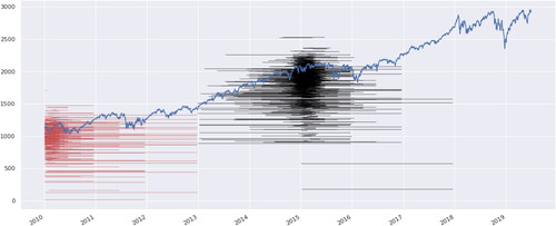
We obtained daily closing bid and ask prices on calls and puts written on the S&P 500 between January 2010 and June 2019 from OptionMetrics (see https://optionmetrics.com). We interpret the midprice as the true market price. Figure 1 displays a sample of the obtained options, namely those puts with price quotes in the first three months of 2010 or 2015. Sensitivities are provided for the majority of options and are filled in for missing values. The results presented below are robust to whether we use computed sensitivities for all options or the sensitivities provided by OptionMetrics where available. The required interest rates are interpolated from the rates provided by OptionMetrics. For maturities less than one week (in which case OptionMetrics does not provide the corresponding rates), we use the Overnight Libor Rates from Bloomberg.

Fig. 1 A sample of the obtained put options along with the underlying’s (S&P 500) price process in blue. Only options that have a trading volume of more than 1000 on some trading day are included. Each red (black) line segment represents a put option that had price quotes within the first quarter of 2010 (2015). The corresponding strike is indicated as the value on the y-axis. Small random vertical shifts are added to increase the visibility of the options.

We organized the data in a table so that each row corresponds to exactly one observation, that is, one option at one trading day (along with the tomorrow’s price for training). We remove certain samples; for example, those samples with negative time-value, time-to-maturity less than 1 day, or zero trading volume. We present the full cleaning process in online Appendix C.1.

2.2 Euro Stoxx 50 Tick Data

We are grateful to Deutsche Börse, who provided us with tick data of Euro Stoxx 50 index options and futures between January 2016 and July 2018. We refer to https://datashop.deutsche-boerse.com/samples-dbag/File_Description_Eurex_Tick.pdf for a description of this dataset.

We now briefly outline how we process these data. If several trades are executed at exactly the same time stamp, then we aggregate these orders and consider the volume-weighted average price. We match each option transaction with the most recent tick price of the future with the shortest maturity (again, volume-weighted if several trades happen simultaneously). These futures, which are the most liquid ones, shall be used to hedge the option position. The computation of the option sensitivities requires a risk-free rate. We use interpolated Euro LIBOR rates from Thomson Reuters’ DataStream.

To train the statistical models and to measure the hedging performance, we require the option price after $\Delta t$ (1 h, 1 day, 2 days, etc.). There might not be a trade exactly after this time period. Hence, we allow a matching tolerance window of 6 min, equivalent to 0.1 hr. Hence, for example, if $\Delta t$ is a business day and we have a trade on Monday, say at 2.12 p.m., then we match it with the first price observation of this option on Tuesday after 2.12 p.m. If there is no transaction before 2:18 p.m., then this sample gets discarded. We refer to Section 5.3 for a discussion of potential information leakage introduced in this step.

Finally, we perform a similar cleaning process as for the S&P 500 dataset. The details are laid out again in online appendix C.1.

2.3 Data Preparation and Experimental Setup

As discussed in Section 1, our goal is to determine the hedging ratio δ as a function of observable quantities to minimize the variance over one period of the hedged portfolio(5) $$V_1^{\delta }=\delta S_1+(1+r_{\text{onr}}\Delta t)(C_0-\delta S_0)-C_1.$$(5)

Here, S₀ and S₁ denote the prices of the hedging instrument at the beginning and end of the period and C₀ and C₁ denote the prices of the call or put. We study how well an ANN performs in this task on end-of-day midprices (see Section 2.1) and on tick data (see Section 2.2). We benchmark these results with linear regression models for the hedging ratio δ. A corresponding simulation study is discussed in online Appendix A.

Each of the datasets is split up into in-sample and out-of-sample (“test”) data. Both the ANN and the benchmark models are trained to (estimated by) the in-sample dataset only. The variance of the hedged portfolio is approximated by the MSHE. The performance of each of the methods is measured on the out-of-sample dataset as follows:(6) $$\text{var}(V_1^{\delta })\approx \text{MSHE}=\frac{1}{N_{\text{test}}}\sum _{t,j}^{N_{\text{test}}}{\left(100\frac{V_{t+1,j}^{\delta }}{S_t}\right)}^2,$$(6) where δ is either modeled by an ANN or by a linear regression. Both the indexing and the normalization by $S_t/100$ need explanation.

First of all, the indexing has changed from Equation (5)(5) $$V_1^{\delta }=\delta S_1+(1+r_{\text{onr}}\Delta t)(C_0-\delta S_0)-C_1.$$(5) to (6)(6) $$\text{var}(V_1^{\delta })\approx \text{MSHE}=\frac{1}{N_{\text{test}}}\sum _{t,j}^{N_{\text{test}}}{\left(100\frac{V_{t+1,j}^{\delta }}{S_t}\right)}^2,$$(6) . Indeed, each traded option yields a series of samples, one for each trading period. Moreover, several options corresponding to different strikes (indexed by j) are being priced in any specific period (e.g., a day). To emphasize this point, the samples are double indexed in Equation (6)(6) $$\text{var}(V_1^{\delta })\approx \text{MSHE}=\frac{1}{N_{\text{test}}}\sum _{t,j}^{N_{\text{test}}}{\left(100\frac{V_{t+1,j}^{\delta }}{S_t}\right)}^2,$$(6) . Next, Equation (6)(6) $$\text{var}(V_1^{\delta })\approx \text{MSHE}=\frac{1}{N_{\text{test}}}\sum _{t,j}^{N_{\text{test}}}{\left(100\frac{V_{t+1,j}^{\delta }}{S_t}\right)}^2,$$(6) normalizes the value of the hedging portfolio by dividing it by $S_t/100$. This normalization “removes the units” and allows to compare errors across the different datasets, and arguably more importantly, across time. Equivalently, at any point of time t, instead of replicating a full option, we replicate the fraction $100/S_t$ of this option.

One could have considered a different normalization. For example, in Equation (6)(6) $$\text{var}(V_1^{\delta })\approx \text{MSHE}=\frac{1}{N_{\text{test}}}\sum _{t,j}^{N_{\text{test}}}{\left(100\frac{V_{t+1,j}^{\delta }}{S_t}\right)}^2,$$(6) , one could have divided by the time-t-option price C_t instead of S_t. This would induce a different weighting of the samples. However, a fixed Dollar position in a far out-of-the money option is riskier than in an at-the-money option. Indeed, a move in the underlying tends to have a larger effect on the far out-of-the money position. Hence, from a risk perspective, the alternative normalization would put too much weight on far out-of-the money options. For this reason, we choose the normalization of Equation (6)(6) $$\text{var}(V_1^{\delta })\approx \text{MSHE}=\frac{1}{N_{\text{test}}}\sum _{t,j}^{N_{\text{test}}}{\left(100\frac{V_{t+1,j}^{\delta }}{S_t}\right)}^2,$$(6) .

We now provide more details on how we prepare each dataset. First, we store each dataset in a dataframe as in Table 1. We then remove all in-the-money samples. That is, if at one specific date an option was in the money, we discard this specific date for the corresponding option.

Table 1 This table presents a (simplified) preview of one of the four processed datasets.

Index	Date	Features				Additional information					Target
		${\sigma }_{\text{impl}}\sqrt{\tau }$	M	${\delta }_{\text{BS}}$	${\mathcal{V}}_{\text{BS}}$	S0	S1	C0	$r_{\text{onr}}$	CP flag	C1
0	2018/07/02	0.047	1.003	0.531	9.357	100	98.223	2.002	0.01	0	1.130
$⋮$

NOTES: The “Features” columns are used as inputs for the ANN and the linear regressions. The labels ${\sigma }_{\text{impl}}\sqrt{\tau }$ and M denote the square root of total implied variance and moneyness of the option. The labels ${\delta }_{\text{BS}}$ and ${\mathcal{V}}_{\text{BS}}$ are the BS Delta and Vega. The CP flag indicates whether the corresponding option is a call or a put. Prices and sensitivities are all normalized.

We break up the S&P 500 dataset in 14 overlapping time windows of length 3 years in order to understand whether the comparisons between the ANNs and the linear regressions are consistent across time. In each time window, the first 900 days form the in-sample set, while the last 180 days are used for the out-of-sample set, yielding a ratio 5:1. For the training of the ANN, the 900 days are furthermore split into 720 days of training and 180 days of validation yielding a ratio 4:1:1. We roll the time windows forward by 180 days, so that sample appears maximally once in the aggregated out-of-sample set. The Euro Stoxx 50 dataset is much shorter, and we do not break it up in different time windows. This leads to 750 (600 + 150) days in the in-sample set and 150 days in the out-of-sample set, yielding again a ratio 4:1:1.

In practice, one would expect to retrain each statistical model weekly or daily instead of every 180 days as done in the S&P dataset. For computational limitations, we are not able to do so. (Currently, training and running one ANN configuration for the 14 S&P time windows takes about 10 hr on a GTX 1060 6GB GPU cluster.) We treat the statistical benchmark models below in the same way, also only retraining them every 180 days.

2.4 Digression: Economic Interpretation of the MSHE

We now briefly comment on the economic gains when using hedging strategies that lead to reduced MSHEs. We have in mind a financial entity (or “operator”) acting as a market maker; that is, taking on (short) positions in options as “inventory” to satisfy some market demand. This operator sells a cross section of delta-hedged puts or calls. In the classical one-period framework of Stoll (1978) (see also (O’Hara 1997, chap 2.2)), the operator charges a premium (e.g., through a bid–ask spread) to take on the additional inventory (i.e., the short position of delta-hedged options). Reducing the MSHE allows the operator to charge a lower premium as we outline next.

Formally, we equip the operator with quadratic utility $x\mapsto x-\gamma x^2/2$, where $\gamma >0$ denotes her coefficient of risk aversion. We suppose that the delta-hedged short-position is uncorrelated with the operator’s optimal wealth. Furthermore, we assume that the expected return of a delta-hedged option position does not depend on the hedging strategy (e.g., if the expected return of the risky asset equals the risk-free return) and set it to zero for simplicity. Under Bertrand competition of liquidity providers with the same risk aversion γ, the operator charges $\gamma /2$ times the MSHE as a premium. Hence, if the MSHE can be reduced by a certain percentage, then the premium reduces by the same percentage times $\gamma /2$. For example, if the MSHE error is reduced by 15% and γ = 2, then the premium decreases by 15%.

A similar argument applies if the financial entity was on the “buy-side,” taking on short positions in options to collect the volatility risk premium, and interested in maximizing the Sharpe ratio of her position. This entity would then try to hedge the exposure to the price movements in the underlying by trading it. If the expected return of a delta-hedged option position does not depend on the hedging strategy and the MSHE is reduced by 15%, then the new Sharpe ratio is $1/\sqrt{0.85}\approx 1.085$ times the old one.

3 HedgeNet

There exists a long line of research on the use of ANNs in the context of option pricing and hedging. Ruf and Wang (2020) provided an overview of this literature. Here, we only give a few pointers to articles that we found especially insightful. Early on, Hutchinson, Lo, and Poggio (1994) suggested ANNs as nonparametric alternative for the pricing of options. They show that already quite small ANNs with only a few nodes perform well for the pricing task. Garcia and Gençay (2000) are among the first to introduce financial domain knowledge (the so-called homogeneity hint) in the design of ANNs. This type of regularization improves the pricing performance of ANNs further. Carverhill and Cheuk (2003) proposed an ANN that directly outputs hedging strategies, instead of the first outputting option prices and then deriving hedging strategies as sensitivities. Dugas et al. (2009) suggested an ANN architecture that guarantees that the outputted prices satisfy a set of no-arbitrage conditions. Buehler et al. (2019) brought several innovations forward. In order to train their ANN, additional artificial data are drawn from an appropriately fitted econometric model. Their framework for hedging options includes the presence of transaction costs and other market frictions, allowing general convex risk measures as loss functions. All these references discussed here consider the pricing/hedging task over the lifespan of an option.

We now introduce the ANN used in this study. As discussed in the introduction, we focus on the one-period setup, and benchmark the hedging performance of the ANN with appropriate linear regressions based on the options’ sensitivities, as described in the next section. The ANN maps the option’s relevant features (e.g., moneyness and square root of total implied variance) to a hedging ratio ${\delta }_{\text{NN}}$. In Section 3.1 we provide details about the architecture, implementation, and training of such an ANN. Section 3.2 provides some additional motivation why the ANN is designed to output directly the hedging ratio instead of the option price.

3.1 Architecture of HedgeNet, Its Implementation and Training

An ANN is a composition of simple elements called neurons, which maps input features to outputs. Such an ANN then forms a directed, weighted graph.

As we shall discuss below in Section 3.2 it is not satisfactory to compute or estimate option prices and then use their sensitivities as hedging ratios. It is better to obtain the hedging ratio, our quantity of interest, directly. Hence, we desire that the ANN returns a hedging ratio and not a price. However, when training such an ANN what should it be trained to? Optimal hedging ratios are not provided in the data. For this reason, we design an ANN, named HedgeNet, to have two parts, as illustrated in Figure 2.

Fig. 2 A schematic graph of HedgeNet. The features are transformed into a hedging position by a fully connected feed-forward neural network (FCNN). The additional input is used to compute the value ${\widehat{C}}_1$ of the replicating portfolio.

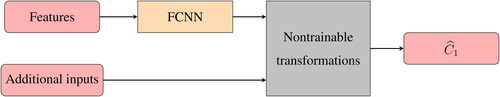
The first part, a multilayer fully connected feed-forward neural network (FCNN), transforms features into a hedging position, which is then turned by the second part into the replication value ${\widehat{C}}_1=V_1+C_1$. This output of HedgeNet can then be trained to the observed option prices C₁ at the end of each period by minimizing the sum of squared differences.

The FCNN has two hidden layers with 30 nodes each, connected by ReLU activation. (The benefits of using ReLU activation are addressed in Glorot, Bordes, and Bengio (2011) and (Krizhevsky, Sutskever, and Hinton 2012, sec. 3.1).) The output of the FCNN is provided by a linear node (with truncation at zero and one) and corresponds to the hedging ratio ${\delta }_{\text{NN}}$. We tried different architectures, for example, 100 nodes in each hidden layer, or three (instead of two) hidden layers with 30 nodes each. Motivated by the representation of the BS Delta in Equation (3)(3) $${\delta }_{\text{BS}}=\mathbf{N}(d_1),$$(3) , we also tried the cumulative distribution function N of a standard normally distributed random variable as output function instead of the linear output function. None of these modifications changed the overall conclusions below. We also tried a modification, where we interpret the output not as the hedging ratio but as the “bias” term $\delta -{\delta }_{\text{BS}}$, which corrects the BS Delta. Such change did not help the performance of the ANN either.

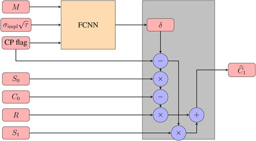
As illustrated in Figure 3, the nontrainable transformation module turns the hedging ratio ${\delta }_{\text{NN}}$ into the replication value ${\widehat{C}}_1$ by following Equation (1)(1) $$V_1^{\delta }=\delta S_1+(1+r_{\text{onr}}\Delta t)(C_0-\delta S_0)-C_1,$$(1) . As the data include both puts and calls, this module also requires an option type flag, which is set to 1 in the case of a put and to 0 in the case of a call. If the sample is a put, then the module replaces ${\delta }_{\text{NN}}$ by ${\delta }_{\text{NN}}-1$ in line with put-call parity. The nontrainable transformation module consists of a series of affine transformations, and hence does not affect the universal approximation property, discussed, for example, in Yarotsky (2017).

Fig. 3 A detailed schematic presentation of HedgeNet. Recall that $M=S_0/K$ and ${\sigma }_{\text{impl}}\sqrt{\tau }$ are moneyness and square root of total implied variance. “CP flag” is a Boolean flag for the option type; it equals 1 for puts and 0 for calls. Next, S₀ and S₁ are the underlying’s prices at the beginning and end of the hedging period, C₀ denotes the option price at the beginning of the period, and ${\widehat{C}}_1$ denotes the replication value. Finally, $R=1+r_{\text{onr}}\Delta t$ is the risk-free overnight return.

All numerical experiments are run on a standard desktop with GPU accelerated computation (specification: GTX 1060 6GB GPU). We use Python as programming language. The ANN is implemented with the deep learning framework Tensorflow along with Keras. The inputs to the trainable part of HedgeNet are standardized. The weights of the ANN are initialized via the “Xavier” initializer (Glorot and Bengio 2010) and the “Adam” optimizer (Kingma and Ba 2015) is applied for training the ANN. Online Appendix B contains details on the choice of additional hyperparameters.

For each dataset, we consider three different feature sets for the trainable part of HedgeNet:

• $\text{ANN}(M;{\sigma }_{\text{impl}}\sqrt{\tau })$: The first one is already indicated in Figure 3. It uses moneyness M, square root of total implied variance ${\sigma }_{\text{impl}}\sqrt{\tau }$, and a flag to indicate whether the option is a call or a put. It is worth pointing out that using moneyness instead of the underlying’s price and the strike price separately offers a better generalization performance. The most important reason for its better performance is that moneyness resembles more a stationary feature compared to the underlying’s price and strike price separately. Indeed, options are created and traded only for a certain range of moneyness values. Ghysels et al. (1998), Garcia and Gençay (2000), and Ruf and Wang (2020) provided more comments on the advantage of using moneyness. The choice of square root of total implied variance is motivated by the fact that volatility squares with the square root of time; see also the expression for ${\delta }_{\text{BS}}$ in Equations (3)(3) $${\delta }_{\text{BS}}=\mathbf{N}(d_1),$$(3) and (4)(4) $$d_1=\frac{1}{{\sigma }_{\text{impl}}\sqrt{\tau }}\left[\text{ln}\hspace{0.17em}\left(\frac{S_0}{K}\right)+\left(r+\frac{1}{2}{\sigma }_{\text{impl}}^2\right)\tau \right].$$(4) .

• $\text{ANN}({\Delta }_{\text{BS}};{\mathcal{V}}_{\text{BS}};\tau )$: Motivated by the leverage effect discussed in Section 4, we also consider the second set of features consisting of ${\delta }_{\text{BS}},{\mathcal{V}}_{\text{BS}},1/\sqrt{\tau }$, and the put-call flag. Here, ${\mathcal{V}}_{\text{BS}}$ denotes Vega, the sensitivity of the option price with respect to the implied volatility.

• ANN(${\Delta }_{\text{BS}};{\mathcal{V}}_{\text{BS}};{\text{Va}}_{\text{BS}};\tau$): Since we shall use Vanna, the sensitivity of Delta with respect to volatility, as a feature for linear regression benchmarks in Section 4, we also consider using a third feature set consisting of the three sensitivities, $1/\sqrt{\tau }$, and the put-call flag.

3.2 Digression: Why Outputting the Hedging Ratio Instead of Computing Price Sensitivities?

Most ANNs constructed in the literature for the risk management of options first learn the pricing function. Then in a second step hedging strategy is computed as the sensitivity of the option price with respect to the underlying’s price; see Ruf and Wang (2020) for an overview of the literature. In contrast, HedgeNet allows to predict the hedging position directly. In this way, the hedging strategy is no longer interpreted as a sensitivity.

From a risk-management point of view, the hedging ratio is the main quantity of interest. It is recommended—see, for example, Bengio (1997) or Claeskens and Hjort (2003)—to estimate relevant quantities directly. This is in line with the important observation made in Lyons (1995) that different models might yield similar option prices but completely different hedging strategies. Obtaining directly the hedging ratio also avoids the otherwise necessary step to differentiate, possibly numerically, the trained option prices.

There are further important advantages of outputting directly the hedging ratio. Computing sensitivities usually does not take into consideration that other model parameters also might change, in line with the underlying. Hence, such sensitivities tend to be not optimal for reducing the MSHE. Theoretical results supporting this observation are ample; see, for example, Denkl et al. (2013). This discussion is continued in Section 4.2. Moreover, as Buehler et al. (2019) showed, training to hedging ratios allows to incorporate market frictions conveniently.

At this point, let us also mention a different approach to use ANNs in the context of option pricing, namely as computational tools to replace expensive PDE solvers or Monte-Carlo simulations. Indeed, the risk management of “sell-side institutions” is subject to regulatory purposes. In particular, their options’ hedging is supposed to be derived from specific parametric models. ANNs are used to estimate (“calibrate”) these model parameters. For references using this approach, see Ruf and Wang (2020). Here, however, we do not intend to study the question how well models can be calibrated by the use of ANNs. Instead, we show the limitations and benefits of ANNs for estimating the optimal hedging ratio when not being restricted by a specific parametric model.

4 Linear Regression Models as Benchmarks

We now discuss how we benchmark the hedging performance of the ANN. Although not very reasonable, one benchmark could be not hedging at all, that is, δ = 0. In this case, the variance of the hedging error is just the variance of the change in the option price. More reasonable is to use the BS Delta, obtained from the Black–Scholes formula, as discussed in Section 4.1. Sections 4.2 and 4.3 introduce some further simple statistical hedging models.

4.1 Black-Scholes Benchmark

Hedging via the BS Delta is a standard benchmark. That is, for each option and for each date the corresponding implied volatility is used to obtain the hedge in Equation (3)(3) $${\delta }_{\text{BS}}=\mathbf{N}(d_1),$$(3) , namely the partial derivative of the Black–Scholes option price with respect to the price of the underlying. Black–Scholes performs the best if implied volatility is plugged in. In the literature, other volatilities, such as historical volatility estimates or GARCH predicted volatilities have been used. We refer to Ruf and Wang (2020) for an overview.

Since here we hedge only discretely, using the BS Delta leads to an error even if the data are simulated from the Black–Scholes model. The performance of discrete-time hedging has been extensively studied; some pointers to the literature include Boyle and Emanuel (1980), Bertsimas, Kogan, and Lo (2000), and Tankov and Voltchkova (2009), who provided an asymptotic analysis of hedging errors.

4.2 Delta Hedging Other Sensitivities

The leverage effect, first discussed in Black (1976), describes the negative correlation of observed returns and their volatilities in equity markets. This effect has been confirmed in many follow-up studies which also consider implied volatilities. For example, Cont and Da Fonseca (2002) claimed that the leverage effect is due to a shift in the overall level of the implied volatility surface and not due to relative movements, that is, changes in the shape of the implied volatility surface. The nonzero correlation of returns and the implied option volatilities indicates that the BS Delta can usually be outperformed by some relatively simple adjustments. In this spirit, Vähämaa (2004) and Crépey (2004) used the observed smile in option implied volatilities to improve on the hedging performance of the BS Delta. These ideas are developed further in several articles; see, for example, Alexander et al. (2012).

The central idea is to note that the first-order Taylor series expansion of option prices yields$$\mathrm{d}C\approx {\delta }_{\text{BS}}\mathrm{d}S+{\mathcal{V}}_{\text{BS}}\mathrm{d}{\sigma }_{\text{impl}}={\delta }_{\text{BS}}\mathrm{d}S+{\mathcal{V}}_{\text{BS}}\frac{\mathrm{d}{\sigma }_{\text{impl}}}{\mathrm{d}S}\mathrm{d}S+{\mathcal{V}}_{\text{BS}}\mathrm{d}{S}^{\perp },$$where $S^{\perp }$ is orthogonal to S. In words, the change in the option price is approximately the BS Delta times the change in the underlying’s price plus Vega times the change in the implied volatility. The second term can be written in terms of changes in the underlying’s price and changes in the implied volatility that are uncorrelated with the changes in the underlying’s price. These observations lead us to consider a statistical model of the form$$\delta =a{\delta }_{\text{BS}}+b{\mathcal{V}}_{\text{BS}}.$$

This statistical model replaces the BS Delta by a multiple a of it plus a multiple b of Vega ${\mathcal{V}}_{\text{BS}}$. Here, a and b are estimated in the in-sample set, separately for puts and calls. More precisely, estimating a and b is equivalent to running a linear regression with two independent variables and no intercept on the in-sample set. Indeed, we minimize the expression in Equation (6)(6) $$\text{var}(V_1^{\delta })\approx \text{MSHE}=\frac{1}{N_{\text{test}}}\sum _{t,j}^{N_{\text{test}}}{\left(100\frac{V_{t+1,j}^{\delta }}{S_t}\right)}^2,$$(6) , where each summand can be written as the square of$$a\left({\delta }_{\text{BS},t,j}{x}_t\right)+b\left({\mathcal{V}}_{\text{BS},t,j}{x}_t\right)-y_{t,j},$$with $x_t=100(S_{t+1}/S_t-(1+r_{\text{onr}}\Delta t))$ and $y_{t,j}=100/S_t(C_{t+1,j}-(1+r_{\text{onr}}\Delta t)C_{t,j})$.

Next, a Taylor series expansion of the BS Delta yields$$\mathrm{d}\delta \approx {\Gamma }_{\text{BS}}\mathrm{d}S+{\text{Va}}_{\text{BS}}\mathrm{d}{\sigma }_{\text{impl}}.$$

Here, ${\Gamma }_{\text{BS}}$ denotes Gamma, namely the sensitivity of the BS Delta to changes in the underlying’s price; ${\text{Va}}_{\text{BS}}$ denotes Vanna, namely the sensitivity of the BS Delta to changes in the implied volatility.

Combining these two expansions we obtain the linear regression model(7) $${\delta }_{\text{LR}}=a{\delta }_{\text{BS}}+b{\mathcal{V}}_{\text{BS}}+c{\text{Va}}_{\text{BS}}+d{\Gamma }_{\text{BS}}.$$(7)

Again, $a,b,c,\text{and},d$ are estimated for puts and calls separately on each in-sample set. We also consider nested models; in this case, we force either a to be one or one (or more) of the other coefficients to be zero and estimate the remaining coefficients. The Vega and Gamma sensitivities are large for options when the strike is close to the underlying’s current price. Thus, including these sensitivities allow the statistical model to make adjustments to the hedging ratio depending on whether an option is at-the-money or out-of-the money. Using both two sensitivities helps, moreover, to make additional adjustments depending on the option’s time-to-maturity. Finally, Vanna for an out-of-the money option is largest when the option is somehow out-of-the-money but not too much. This allows the model to make the corresponding additional adjustments. We have also experimented with an additional intercept term in Equation (7)(7) $${\delta }_{\text{LR}}=a{\delta }_{\text{BS}}+b{\mathcal{V}}_{\text{BS}}+c{\text{Va}}_{\text{BS}}+d{\Gamma }_{\text{BS}}.$$(7) . Including it does not change the conclusions below; we hence only report the results without this additional term.

Furthermore, we include below the proposed hedging ratio of Hull and White (2017), given by(8) $${\delta }_{\text{HW}}={\delta }_{\text{BS}}+\frac{{\mathcal{V}}_{\text{BS}}}{\sqrt{\tau }S}(a+b{\delta }_{\text{BS}}+c{\delta }_{\text{BS}}^2).$$(8)

Here, τ is the time-to-maturity and $a,b,\text{and}c$ are again estimated for puts and calls separately on each in-sample set. Hull and White (2017) obtained this model from a careful analysis of S&P 500 options and observe its excellent hedging performance on options written on the S&P 500 and other indices. We furthermore include a “Relaxed Hull-White” model, where the coefficient in front of ${\delta }_{\text{BS}}$ is not restricted to one.

The models in Equations (7)(7) $${\delta }_{\text{LR}}=a{\delta }_{\text{BS}}+b{\mathcal{V}}_{\text{BS}}+c{\text{Va}}_{\text{BS}}+d{\Gamma }_{\text{BS}}.$$(7) and (8)(8) $${\delta }_{\text{HW}}={\delta }_{\text{BS}}+\frac{{\mathcal{V}}_{\text{BS}}}{\sqrt{\tau }S}(a+b{\delta }_{\text{BS}}+c{\delta }_{\text{BS}}^2).$$(8) should be considered “statistical” in contrast to “model-driven” as the hedging ratio is derived purely from statistical considerations instead of being derived from stochastic models. In the language of Carr and Wu (2020), these models are “local” and “decentralized,” as only one period is considered instead of the option’s whole time horizon, and as each option contract is treated separately instead of finding an overall consistent valuation model. To the best of our knowledge, the model in Equation (7)(7) $${\delta }_{\text{LR}}=a{\delta }_{\text{BS}}+b{\mathcal{V}}_{\text{BS}}+c{\text{Va}}_{\text{BS}}+d{\Gamma }_{\text{BS}}.$$(7) has not been suggested in the literature before, despite its simplicity. Relatedly, Bergomi (2009) introduced the “skew stickiness ratio” to describe the idea that changes in the at-the-money implied volatility relative to the underlying’s logarithmic return is proportional to the implied at-the-money volatility skew. The proportionality constant can then be estimated again by linear regression. In the context of credit risk, Cont and Kan (2011) also provided a careful study of regression-based hedging. While here the hedging ratio is regressed on option sensitivities, they regress changes in the option price on changes in the underlying.)

4.3 Possible Other Benchmarks

One could consider hedging ratios derived from parametric models such as stochastic volatility models. Bakshi, Cao, and Chen (1997) observed that such models outperform the BS Delta in the case of hedging out-of-the money options, but not necessarily in-the-money options. Vähämaa (2004) provided additional references that test the hedging performance of stochastic volatility models and concludes with the observation that “such models do not necessarily provide better hedging performance.” Hull and White (2017) noted that the hedging ratio ${\delta }_{\text{HW}}$ of Equation (8)(8) $${\delta }_{\text{HW}}={\delta }_{\text{BS}}+\frac{{\mathcal{V}}_{\text{BS}}}{\sqrt{\tau }S}(a+b{\delta }_{\text{BS}}+c{\delta }_{\text{BS}}^2).$$(8) leads to a better performance than stochastic volatility models.

We initially also investigated the following two (semi-)linear benchmarks:$${\overline{\delta }}_1=aM+b{\sigma }_{\text{impl}}\sqrt{\tau }+c;\mathrm{\hspace{1em}}\mathrm{\hspace{1em}}{\overline{\delta }}_2=\mathbf{N}\left(aM+b{\sigma }_{\text{impl}}\sqrt{\tau }+c\right),$$where M denotes moneyness, ${\sigma }_{\text{impl}}\sqrt{\tau }$ square root of total implied variance, and N the cumulative normal distribution function. Here, the parameters a, b, c were estimated again in each in-sample set. It turns out that these two linear regressions perform far worse than the BS Delta ${\delta }_{\text{BS}}$; hence, we will not present results on these two benchmarks. The underperformance of these two linear regressions also shows that the performance of the ANN is not entirely due to the hand-crafted features.

5 Results

We now present the results on the performance of the various statistical hedging models in terms of MSHE reduction. As a quick summary, the hedging ratios of the ANNs do not outperform the linear regression models. On the S&P 500 dataset, the Hull-White and Delta-Vega-Vanna regressions tend to perform the best, with Hull-White better on the one-day hedging period, and the Delta-Vega-Vanna regression better on the two-day period. On the Euro Stoxx 50 dataset, the Delta-Vega-Gamma-Vanna regression tends to perform the best. However, the differences between these linear regressions with three or four coefficients are neither statistically nor economically significant, as we shall discuss.

Recall from Section 2.3 that each data sample is normalized so that the underlying’s price S₀ at time 0 is 100. This allows to compare the absolute hedging errors across different datasets. Recall also that we only consider out-of-the (and at-the)-money puts and calls. In the next two subsections, we discuss the results for the S&P 500 and Euro Stoxx 50 datasets. In Section 5.3, we conclude this section with some general observations and guidelines.

5.1 S&P 500 End-of-Day Midprices

Table 2 gives an overview of the MSHEs across different hedging periods. The first two rows give the MSHEs for the zero hedge and the BS Delta. The remaining rows give the relative improvement over the BS Delta, that is,(9) $$\frac{\text{MSHE}({\delta }_{*})-\text{MSHE}({\delta }_{\text{BS}})}{\text{MSHE}({\delta }_{\text{BS}})},$$(9)

Table 2 Performance of the linear regressions and ANNs on the S&P 500 dataset.

		1 day			2 days
		Calls	Puts	Both	Calls	Puts	Both
	Zero hedge	4.01	4.78	4.54	8.31	9.73	9.29
	BS Delta	0.687	0.655	0.665	1.58	1.54	1.55
$\begin{array}{c}\hfill \\ \hfill \\ \hfill \\ \hfill \\ \hfill \\ \hfill \\ \hfill \\ \hfill \\ \hfill \\ \hfill \\ \hfill \\ \hfill \end{array}\text{Regressions}\{$	Delta-only	–21.3	–14.8	–16.9	–16.3	–12.8	–13.9
	Vega-only	–13.7	–11.7	–12.3	–10.4	–10.1	–10.2
	Gamma-only	–15.5	–10.1	–11.8	–14.5	–11.2	–12.2
	Vanna-only	–12.4	–12.6	–12.5	–10.6	–13.0	–12.2
	Delta-Gamma	–21.6	–14.8	–17.0	–17.1	–13.1	–14.4
	Delta-Vega	– 21.4	– 14.9	– 17.0	– 16.4	– 12.8	– 13.9
	Delta-Vanna	–22.6	–16.6	–18.5	–17.7	–15.4	–16.1
	Delta-Vega-Gamma	–21.5	–14.8	–17.0	–16.8	–13.5	–14.5
	Delta-Vega-Vanna	–23.0	–16.6	–18.7	–18.1	–15.4	–16.2
	Delta-Gamma-Vanna	–22.6	–16.6	–18.5	–17.7	–15.2	–16.0
	Delta-Vega-Gamma-Vanna	–22.9	–16.4	–18.5	–17.4	–14.9	–15.7
	Hull-White	–23.1	–16.9	–18.9	–17.8	–14.5	–15.5
	Relaxed Hull-White	–23.2	–16.9	–18.9	–18.3	–14.6	–15.8
$\begin{array}{c}\hfill \\ \hfill \end{array}\text{ANNs}\{$	$M;{\sigma }_{\text{impl}}\sqrt{\tau }$	–22.3	–15.6	–17.7	–17.1	–10.9	–12.8
	${\Delta }_{\text{BS}};{\mathcal{V}}_{\text{BS}};\tau$	–23.4	–16.9	–18.9	–18.6	–12.9	–14.7
	${\Delta }_{\text{BS}};{\mathcal{V}}_{\text{BS}};{\text{Va}}_{\text{BS}};\tau$	–21.9	–14.4	–16.8	–12.5	–12.9	–12.8

NOTES: The hedging periods $\Delta t$ are here either one day or two days. The columns “Both” are the weighted average of the “Puts” and “Calls” columns. The row “Zero hedge” corresponds to the MSHE when δ = 0 is chosen; that is, the mean squared changes in the option prices. The values in the top two rows are multiplied by 100 to improve readability. The regression and ANN rows correspond to the various statistical models including HedgeNet with three different feature sets. For these two sets of rows, the numbers are reported as relative improvements in MSHE over using the BS Delta, that is, Equation (9)(9) $$\frac{\text{MSHE}({\delta }_{*})-\text{MSHE}({\delta }_{\text{BS}})}{\text{MSHE}({\delta }_{\text{BS}})},$$(9) . Numbers in bold represent the largest outperformance (in each column the best one is chosen along with the ones that are within 1% of the best).

All competing methods outperform the BS Delta. Among them, the Delta-Vega-Vanna and (relaxed) Hull-White regressions perform the best, with Hull-White doing slightly better on the one-day hedging period while Delta-Vega-Vanna performing better on two-day hedging period. Indeed, Hull and White (2017) studied the same dataset to create the Hull-White regression, so it is surprising how close the other regressions get. The major improvement in the regressions (apart from the Hull-White regression) comes from allowing the coefficient in front of Delta to be estimated, rather than equal to one. The ANNs perform similarly to the regressions in case of the one-day period, but underperform for the two-day period.

Table 2 indicates that it is easier to outperform the BS Delta when hedging out-of-the money calls than out-of-the money puts. However, note that the BS Delta itself reduces the MSHE more for puts than for calls when using the zero hedge as baseline. To see this, let us have a closer look at the one-day period. For calls, hedging with the BS Delta reduces the MSHE by $1-0.687/4.01\approx 83\%$, while for puts, it reduces the MSHE by $1-0.655/4.78\approx 88\%$. Using the Hull-White Delta reduces the MSHE for calls only by $1-(1-0.231)\times 0.687/4.01\approx 87\%$, but for puts by $1-(1-0.169)\times 0.655/4.78\approx 89\%$. Hence, the relative outperformance of the linear regressions and ANNs over the BS Delta is higher exactly when the BS Delta has a worse performance. These observations are not due to the asymmetric choice of moneyness (recall that we only consider out-of-the money options with moneyness $M=S_0/K$ between 0.8 and 1 for calls and between 1 and 1.5 for puts). Indeed the same results as outlined in this paragraph hold true when we allow moneyness to be between 0.6 and 1 for calls and restrict it to be between 1 and 1.2 for puts.

Recall from Section 2 that the S&P 500 dataset is been split in rolling windows, each time shifted by 180 days. This yields 14 out-of-sample sets. The samples in each out-of-sample set are evaluated with the model parameters estimated on its corresponding in-sample set. Figure 4 compares the MSHEs of different statistical models by time window. Consistent with Table 2, the blue dots corresponding to the BS Delta are usually the largest. Both Table 2 and Figure 4 show that for two-day hedging period, the MSHEs are about twice those for the one-day period. The only exceptions are the 7th and the 13th time window, when the errors are about 4 times and 3 times larger in the two-day period.

Fig. 4 MSHEs of four different statistical models for the hedging ratio across all 14 time windows in the S&P 500 dataset, for the one-day (left) and two-day (right) hedging period. The in-sample sets for periods 7 and 12 range from 2013 to the first half of 2015 and the second half of 2015 to 2017, respectively. The test data for the 7th time window fall exactly in the 2015–16 selloff. The test data for the 12th time window contain the first week of February 2018, where the S&P 500 experienced a 10% drop; see also Figure 1.

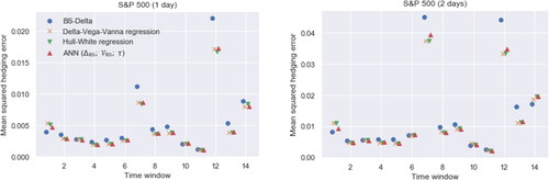
Figure 5 provides the coefficients (plus their standard errors) for the Delta-Vega-Vanna regression in the one-day period setting. The intervals are getting smaller for later time windows due to the fact that later time windows contain more samples as illustrated in Online Appendix C. Especially the Vanna coefficients for calls are very stable across time windows. Figure 4 shows that both the 7th and the 12th time window, whose out-of-sample data are the second half of 2015 and the first half of 2018, respectively, lead to an overall large MSHE. The corresponding samples are then part of the in-sample set for the following periods. And indeed, Figure 5 indicates a jump in some of the coefficients in the 8th and 13th time window.

Fig. 5 The coefficients in the Delta-Vega-Vanna regression for each of the 14 time windows in the S&P 500 dataset. The top and bottom of each line segment are the point estimate plus/minus two standard errors. These numbers correspond to the one-day hedging period. The coefficient plots for the two-day hedging periods (not displayed here) look very similar; in particular, the Vanna coefficients for calls are again stable. However, the Vanna coefficients for puts and the Vega coefficients for calls and puts are slightly more fluctuating.

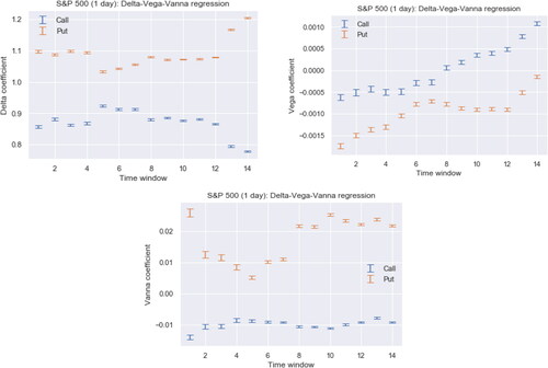
The Delta coefficients of calls being smaller than one implies that hedging a short position on a call, one would usually buy less of the underlying than implied by the BS Delta. On the other hand, for hedging a short position on a put, one needs to short more of the underlying. This phenomenon is consistent with the leverage effect, discussed in Section 4.2. Note that Vanna is positive (negative) for out-of-the money calls (puts). Hence, the Vanna term in the regression further contributes to holding an even smaller number of the underlying than only implied by the Delta term. Since Vanna is largest in absolute value for slightly out-of-the money options, this correction term is largest for such options. The Vega coefficients are negative for puts and most time windows also for calls, adding yet a third correction, most effective for long-dated at-the-money options.

Additional diagnostics are available in online Appendices D and E.

We run three extra experiments to see whether the above conclusions depend on the chosen setup.

1. In the first modified experiment, we remove all options that have a time-to-maturity of 14 calendar days or less from both the in-sample and out-of-sample sets. This yields an additional relative improvement of about 2% in the one-day experiment and about 3% in the two-day experiment for all methods presented in Table 2. We omit presenting the precise numbers here.

2. In the second modified experiment, we abstain from splitting the dataset in 14 time windows. Instead of 14 experiments we hence only have one, but with a much larger number of samples. We keep the ratio 4:1:1, now across the whole dataset, leading to an in-sample set of length 2850 (2280 + 570) days and a test set of length 570 days (instead of 14 test in-sample sets of length 900 (720 + 180) days and an out-of-sample set of length 180 days; see Section 2.3). We omit the detailed results of this experiment. The regression models and ANNs improve their relative performance by about 3% to 4% when using only one time window instead of 14 time windows. Again the ANNs do not outperform the linear regression models.

3. We put the options in two roughly equally sized buckets: at-the-money/close-to-the money options and out-of-the money options. We run the linear regressions and (appropriately tuned) ANNs on both buckets separately. The bucketing tends to help the linear regressions using a single sensitivity slightly, does not change the linear regressions using several sensitivities, and leads to a worse performance of the ANNs.

Section 5.3 provides a fourth experiment to check whether the cleaning process of the raw data introduced any information leakage.

5.2 Euro Stoxx 50 Tick Data

Table 3 shows the performance of all competing methods on the Euro Stoxx 50 dataset. Again we conclude that the ANNs in general do not outperform the linear regressions. Now the Delta-Vega-Gamma-Vanna regression performs best, closely followed by the linear regressions using three sensitivities, which perform better than the Hull-White regressions.

Table 3 Performance of the benchmarks and ANNs on the Euro Stoxx 50 dataset, when the in-sample and out-of-sample are split into one time window.

		1 hr			1 day			2 days
		Calls	Puts	Both	Calls	Puts	Both	Calls	Puts	Both
	Zero hedge	0.431	1.02	0.756	4.28	10.2	7.47	8.20	24.26	17.4
	BS Delta	0.109	0.214	0.167	1.19	1.99	1.62	2.97	4.20	3.67
$\begin{array}{c}\hfill \\ \hfill \\ \hfill \\ \hfill \\ \hfill \\ \hfill \\ \hfill \\ \hfill \\ \hfill \\ \hfill \\ \hfill \\ \hfill \end{array}\text{Regressions}\{$	Delta-only	–18.9	–11.4	–13.6	–21.7	–12.2	–15.4	–36.0	–10.7	–19.5
	Vega-only	–25.3	–13.8	–17.2	–23.4	–16.0	–18.5	–35.2	–16.2	–22.8
	Gamma-only	–0.62	–1.29	–1.10	–15.7	–4.64	–8.37	–32.7	–4.62	–14.4
	Vanna-only	–16.1	–5.18	–8.35	–17.1	–12.6	–14.1	–26.9	–16.9	–20.4
	Delta-Gamma	–18.0	–14.5	–15.5	–20.5	–12.7	–15.4	–33.5	–6.89	–16.1
	Delta-Vega	– 23.9	– 13.7	– 16.7	– 22.7	– 15.4	– 17.9	– 36.9	– 15.3	– 22.8
	Delta-Vanna	–20.8	–11.4	–14.1	–19.2	–14.8	–16.3	–34.9	–17.2	–23.4
	Delta-Vega-Gamma	–21.6	–15.2	–17.0	–20.7	–15.4	–17.2	–34.4	–13.5	–20.8
	Delta-Vega-Vanna	–23.6	–13.7	–16.6	–19.6	–16.7	–17.7	–35.1	–18.5	–24.2
	Delta-Gamma-Vanna	–23.1	–15.5	–17.7	–20.2	–17.9	–18.7	–33.8	–17.7	–23.3
	Delta-Vega-Gamma-Vanna	–23.3	–15.6	–17.8	–20.1	–18.0	–18.7	–34.4	–18.2	–23.9
	Hull-White	–20.0	–12.5	–14.7	–20.7	–14.3	–16.4	–36.1	–13.3	–21.2
	Hull-White-relaxed	–20.3	–12.6	–14.8	–20.6	–14.2	–16.4	–36.1	–12.7	–20.8
$\begin{array}{c}\hfill \\ \hfill \end{array}\text{ANNs}\{$	$M;{\sigma }_{\text{impl}}\sqrt{\tau }$	–17.6	–15.7	–16.3	–8.96	–3.3	–5.21	–27.4	11.3	–2.12
	${\Delta }_{\text{BS}};{\mathcal{V}}_{\text{BS}};\tau$	–16.1	–6.08	–9.01	–19.0	–6.83	–10.9	–25.6	–3.6	–11.2
	${\Delta }_{\text{BS}};{\mathcal{V}}_{\text{BS}};\mathrm{V}{a}_{\text{BS}};\tau$	–25.0	–13.3	–16.7	–18.8	–10.1	–13.1	–29.2	–6.96	–14.7

NOTE: We refer to the caption of Table 2 for an explanation.

Just using the BS Delta reduces the overall MSHE by about 78% and 79%. This percentage is very stable across the three different hedging periods and smaller than in the S&P 500 dataset. Again, the BS Delta reduces the MSHE more for puts than for calls, and the relative outperformance of the regression models is larger when the BS Delta is worse.

We list the coefficients of the Delta-Vega-Gamma-Vanna regression (plus their standard errors) in Table 4. Again, the Delta coefficients for calls (puts) are smaller (larger) than one, consistent with the leverage effect. Additional diagnostics are available in Online Appendices D and F.

Table 4 Coefficients of Delta-Vega-Gamma-Vanna regression for each sensitivity on the Euro Stoxx 50 dataset.

	1 hour		1 day		2 days
	Calls	Puts	Calls	Puts	Calls	Puts
Delta	0.944 ± 0.002	1.134 ± 0.002	0.755 ± 0.003	1.056 ± 0.003	0.821 ± 0.004	1.021 ± 0.003
Vega	$-0.002\pm 0.000$	0.000 ± 0.000	$-0.001\pm 0.000$	$-0.002\pm 0.000$	$-0.001\pm 0.000$	$-0.002\pm 0.000$
Gamma	$-0.021\pm 0.004$	0.213 ± 0.003	$0.226\pm 0.008$	0.393 ± 0.006	0.109 ± 0.010	$0.417\pm 0.008$
Vanna	$-0.010\pm 0.000$	0.014 ± 0.000	0.004 ± 0.000	0.029 ± 0.000	0.003 ± 0.000	0.025 ± 0.000

NOTES: Coefficients are presented for calls and puts separately. Each cell shows the coefficient and its standard error.

Similarly to the S&P 500 dataset we run two additional experiments.

1. In the first one, we only consider options with a time-to-maturity of 14 calendar days or more. This yields an additional relative improvement of about 4–8%, in comparison with Table 3. The improvement tends to be larger for the regressions using a smaller number of sensitivities. In particular, the Delta-Vega-Vanna regression now seems to dominate the Delta-Vega-Gamma-Vanna regression, especially for the two-day hedging period. We again omit the precise numbers here as the overall conclusions do not change.

2. We again put the options in two roughly equally sized buckets: at-the-money/close-to-the money options and out-of-the money options. Running the statistical models on both buckets separately seems to help slightly the linear regressions with only one sensitivity but does not change or worsens the performance of the other linear regressions and ANNs.

We also refer to Section 5.3 for another experiment to check how the cleaning of the data might influence the results of this subsection.

5.3 Guidelines on Statistical Hedging

We now develop some guidelines based on the results of the last two subsections.

In none of the datasets do ANNs outperform the linear regression models. We conclude that the option sensitivities suffice to capture the nonlinearities in the data that are relevant for the hedging task. Additional drawbacks of ANNs are their computational demands and the necessary effort to tune their hyperparameters (see online Appendix B).

Next, we have a closer look at the MSHEs of the linear regression models. To this end, in the spirit of Equation (6)(6) $$\text{var}(V_1^{\delta })\approx \text{MSHE}=\frac{1}{N_{\text{test}}}\sum _{t,j}^{N_{\text{test}}}{\left(100\frac{V_{t+1,j}^{\delta }}{S_t}\right)}^2,$$(6) , let us define the time-t MSHE by$${\text{MSHE}}_t^{\delta }=\frac{1}{N_t}\sum _j^{N_t}{\left(100\frac{V_{t+1,j}^{\delta }}{S_t}\right)}^2,$$where N_t denotes the number of samples at time t. Here, t ranges over days in the test set and δ denotes one of the hedging methods. Hence ${\text{MSHE}}_t^{\delta }$ denotes the average of a cross section of hedging errors, namely those corresponding to the options traded at some time t. Next, for each pair of hedging methods (e.g., the Delta-only and the Delta-Vega-Vanna regressions), we compute an approximate confidence interval for the difference of the MSHEs by adding and subtracting twice the standard error to the mean of the differenced time-t MSHEs. To be more specific, we denote the difference of the MSHEs between two regression models δ_A and δ_B by ${\text{MSHE}}_t^{{\delta }_A-{\delta }_B}={\text{MSHE}}_t^{{\delta }_A}-{\text{MSHE}}_t^{{\delta }_B}$. Then the approximate confidence interval for the two regression methods is given by$$\begin{array}{c}(\frac{1}{T}\sum _{t=1}^T{\text{MSHE}}_t^{{\delta }_A-{\delta }_B}-2*\text{Std}({\text{MSHE}}_t^{{\delta }_A-{\delta }_B}),\\ \hspace{1em}\frac{1}{T}\sum _{t=1}^T{\text{MSHE}}_t^{{\delta }_A-{\delta }_B}+2*\text{Std}({\text{MSHE}}_t^{{\delta }_A-{\delta }_B})),\end{array}$$ where T denotes the number of days in the test set and std denotes the (population) standard deviation.

Due to their possible statistical dependence in time, these confidence intervals need to be interpreted with caution. They allow us to make the following observations.

• For both hedging periods in the S&P 500 dataset, the confidence intervals for time-t MSHEs of BS Delta hedging paired with any of the statistical regressions (except for Gamma-only and Vanna-only regressions) do not contain zero, strongly suggesting that their relative outperformance is not due to noise only. The same observation also holds for the one-hour and two-day hedging periods in the Euro Stoxx 50 dataset. For the one-day hedging period in the Euro Stoxx 50 dataset, the statistical methods reduce the BS Delta hedging error by up to 18.7%, but the corresponding confidence intervals include zero. This gives an instance where the outperformance seems to be economically significant but fails to be statistically significant.

• There is statistical evidence for the underperformance of the Gamma-only and Vanna-only regressions. Pairing them with any of the linear regression models usually leads to confidence intervals that do not include zero. However, among any pairs of the remaining linear regression models the evidence is not clear cut. Sometimes the corresponding confidence intervals contain zero, sometimes they do not.

We recommend to choose one of the linear regression models, for example, the Delta-Vega-Vanna or the Delta-Vega-Gamma-Vanna regressions, which perform best in the above experiments. Let us also note that the choice between the two probably does not matter much from an economic perspective. Indeed, let us consider the one-day hedging period in Euro Stoxx 50, where the two regressions yield a relative reduction of 17.7% and 18.7% (see Table 3). If we now consider the Sharpe ratio of a delta-hedged option as in Section 2.4, then these relative reductions increase the Sharpe ratio by a factor of $1/\sqrt{0.823}\approx 1.10$ and $1/\sqrt{0.813}\approx 1.11$, respectively. While either one leads to an economically significant increase in Sharpe ratio, their relative difference seems to be very minor.

We conclude this section with a further observation. Motivated by the reported results we try another “fixed” hedging strategy that does not require any historical data. All calls are hedged by $0.9*{\delta }_{\text{BS}}$ and puts are hedged by $1.1*{\delta }_{\text{BS}}$. We have not run other such “fixed” hedging strategies (hence, we have not optimized this 10% relative correction term). Table 5 shows the relative performance of this “fixed” strategy with respect to BS Delta on the S&P 500 and Euro Stoxx 50 datasets. The out-of-sample tests are the same ones that were used for Tables 2 and 3. This simple strategy does very well but underperforms the linear regression models.

Table 5 Performance of the “fixed” hedging strategy on the S&P 500 and Euro Stoxx 50 datasets.

	1 hour			1 day			2 days
	Calls	Puts	Both	Calls	Puts	Both	Calls	Puts	Both
S&P 500	–	–	–	–18.6	–13.1	–14.8	–15.0	–11.4	–12.6
Euro Stoxx 50	–15.4	–10.3	–11.8	–15.4	–12.7	–13.6	–23.7	–16.6	–19.0

NOTES: In the “fixed” hedges strategy, calls (puts) are hedged by $0.9*{\delta }_{\text{BS}}$ ($1.1*{\delta }_{\text{BS}}$). See the caption of Table 2 for further explanations.

6 Potential Information Leakage Through Data Cleaning

We next discuss information leakage issues connected to the data cleaning process. One obvious mistake would be removing samples with wrong-way option price changes. An example is the removal of call option samples, whenever the underlying’s price increases but the call price decreases. Although the first thought might be that this is a data issue such samples are very well possible due to changes in the bid–ask spread or due to the leverage effect; see also Bakshi, Cao, and Chen (2000) and Pérignon (2006) for empirical evidence. Another important source for information leakage is introduced if the dataset is split into in-sample and out-of-sample sets without paying respect to the time series structure. This can be mitigated by using a chronological split instead of a random split; see Ruf and Wang (2021).

The availability of end-of-period prices is a more difficult issue to be resolved. Here, in our opinion, information leakage cannot be completely avoided since it is not clear at the beginning of a period whether prices can be observed at its end. If those prices were missing at random, it would be fine to remove those samples during backtesting. However, for financial price data, such an assumption cannot be easily justified. Indeed, missing observations tend to be caused by missing market liquidity. Market liquidity and the implied volatility surface might very well depend on each other. Hence, removing missing observations could potentially lead to biased parameter estimations.

To understand whether information leakage through missing price observations appears in our experiments we run robustness checks for both the S&P 500 and the Euro Stoxx 50 datasets.

We begin with the S&P 500 dataset. For these data, we have quoted prices for all options, along with trading volumes. For the results in Section 5.1, we remove all samples whose trading volume at the beginning of its period are zero. We keep those samples whose volume at the beginning is positive, but zero at the end of the period. As a robustness check we rerun the complete analysis with those samples removed whose trading volume is zero at the end of the period. This reduces the overall dataset by about 22% and increases the MSHE of the zero-hedge for puts (by more than 10%). An explanation for this increase is that this modified cleaning procedure removes especially deep out-of-the-money puts, thus increasing the average squared prices changes. However, the relative performance improvement of the models with respect to the BS Delta does not change much; in particular, the conclusions of Section 5.1 seem to be robust with respect to this cleaning procedure.

Next, let us discuss the Euro Stoxx 50 dataset consisting of tick data. Using such tick data leads to several difficulties concerning missing price observations. First, the underlying’s prices (we use short-term futures on the Euro Stoxx 50) and option prices are not observed synchronously. This issue is relatively mild since futures are extremely liquid. For an option observation at some time t, we thus use the future’s price at the last transaction before t.

However, a major issue in the data cleaning process is to determine the price of the option at the end of a period. To illustrate, consider the one-hour period setup. If an option transaction in the dataset is observed at some time t, then we would like to know the option price at time $t+$1 hour to backtest the hedging performance of the different methods. It is very unlikely to find a trade at exactly this time. To handle this issue, we introduced a matching tolerance window of 6 min (see Section 2.2). That is, if at some time t a transaction occurs then the sample’s end-of-period price is the first price observation after time $t+$1 hour, and the sample is discarded if this end-of-period transaction occurs later than $t+$66 minutes.

As discussed above, we have clearly introduced some information leakage by removing illiquid samples for which no end-of-period price is observed. Let us now do again a robustness check. To this end, we increase the matching tolerance window from 6 to 30 min. In the one-day period situation, this increases the overall number of samples from 0.6 million to 1.4 million, a 133% increase. This modified set contains now many more illiquid options, reflected also in a smaller MSHE of the zero-hedge.

We first summarize how the Delta-Vega-Gamma-Vanna regression performs on this modified and enlarged dataset. For the two-day hedging period, the performance improves on calls but worsens on puts, reducing the overall performance from about –23.9% to –23.0%. For the one-day period, the longer matching tolerance window improves the Delta-Vega-Gamma-Vanna regression by 0.59% with respect to BS Delta, from –18.7% to –19.3%, benefiting both calls and puts. For the one-hour hedging period, the overall performance worsens by 0.1% with respect to BS Delta, from –17.8% to –17.7%, and the longer matching tolerance window benefits calls and not puts. All in all, for the regression models, the conclusions of Section 5.2 are still valid. However, the longer matching tolerance window has a significantly negative effect for the ANNs. Now ANN (${\Delta }_{\text{BS}};{\mathcal{V}}_{\text{BS}};\mathrm{V}{a}_{\text{BS}};\tau$) always produce worse performance for the three hedging periods, up to even a 6% loss in outperformance. Overall, doubling the dataset by increasing the matching tolerance window does not change the regression results much, but significantly handicaps the training of the ANNs. A further test with a matching tolerance window of 60 min leads to the same conclusions.

7 Conclusion and Discussion

In this work, we consider the problem of hedging an option over one period. We consider statistical, regression-type hedging ratios (in contrast to model-implied hedging ratios). To study whether the option sensitivities already capture the relevant nonlinearities we develop a suitable ANN architecture. Experiments involving both quoted prices (S&P 500 options) and high-frequency tick data (Euro Stoxx 50 options) show that the ANNs perform roughly as well (but not better) as the sensitivity-based linear regression models. However, the ANNs are not able to find additional nonlinear features. Hence, option sensitivities by themselves (in particular, Delta, Vega, and Vanna) in combination with a linear regression are sufficient for a good hedging performance.

The linear regression models improve the hedging performance (in terms of MSHE) of the BS Delta by about 15–20% in real-world datasets. An explanation is the leverage effect that allows the partial hedging of changes in the implied volatility by using the underlying. As a rule of thumb, historical data seem to imply that calls should be hedged with about $0.9{\delta }_{\text{BS}}$ and puts with about $1.1{\delta }_{\text{BS}}$. With the presence of sufficient historic data, we recommend to follow a hedging strategy obtained from a linear regression on the BS Delta, BS Vega, BS Vanna, and possibly the BS Gamma.

We have not performed a cross-sectional study where the hedging ratio is estimated not only from options written on the same underlying. It would be interesting to see whether the hedging ratios of the linear regression models can be further improved by using options written on different underlyings, for example, the constituents of an index.

Acknowledgments

We thank Matthias Büchner, Agostino Capponi, Philipp Dörsek, Aleš Černý, Jean-Pierre Fouque, Camilo Garcia, Lukas Gonon, Harald Oberhauser, Philipp Illeditsch, Antoine Jacquier, Johannes Muhle-Karbe, Peter Spoida, Josef Teichmann, and James Wolter for helpful discussions on the subject matter of this article. We are grateful to Deutsche Börse, in particular, Peter Spoida, for providing us with Euro Stoxx 50 options and futures tick data. We are indebted to two anonymous referees and an associate editor for several very insightful comments that improved the article.

References

- Alexander, C., Rubinov, A., Kalepky, M., and Leontsinis, S. (2012), “Regime-Dependent Smile-Adjusted Delta Hedging,” Journal of Futures Markets, 32, 203–229. DOI: 10.1002/fut.20517.
- Bakshi, G., Cao, C., and Chen, Z. (1997), “Empirical Performance of Alternative Option Pricing Models,” The Journal of Finance, 52, 2003–2049. DOI: 10.1111/j.1540-6261.1997.tb02749.x.
- Bakshi, G., Cao, C., and Chen, Z. (2000), “Do Call Prices and the Underlying Stock Always Move in the Same Direction?,” The Review of Financial Studies, 13, 549–584.
- Bengio, Y. (1997), “Using a Financial Training Criterion Rather than a Prediction Criterion,” International Journal of Neural Systems, 8, 433–443. DOI: 10.1142/S0129065797000422.
- Bergomi, L. (2009), “Smile Dynamics IV,” Risk, 22, 94–100.
- Bertsimas, D., Kogan, L., and Lo, A. W. (2000), “When is Time Continuous?,” Journal of Financial Economics, 55, 173–204. DOI: 10.1016/S0304-405X(99)00049-5.
- Black, F. (1976), “Studies of Stock Market Volatility Changes,” Proceedings of the American Statistical Association Business and Economic Statistics Section, pp. 177–181.
- Boyle, P. P., and Emanuel, D. (1980), “Discretely Adjusted Option Hedges,” Journal of Financial Economics, 8, 259–282. DOI: 10.1016/0304-405X(80)90003-3.
- Buehler, H., Gonon, L., Teichmann, J., and Wood, B. (2019), “Deep Hedging,” Quantitative Finance, 19, 1271–1291. DOI: 10.1080/14697688.2019.1571683.
- Carr, P., and Wu, L. (2020), “Option Profit and Loss Attribution and Pricing: A New Framework,” The Journal of Finance, 75, 2271–2316. DOI: 10.1111/jofi.12894.
- Carverhill, A. P., and Cheuk, T. H. (2003), “Alternative Neural Network Approach for Option Pricing and Hedging,” SSRN 480562.
- Claeskens, G., and Hjort, N. L. (2003), “The Focused Information Criterion,” Journal of the American Statistical Association, 98, 900–916. DOI: 10.1198/016214503000000819.
- Cont, R., and Da Fonseca, J. (2002), “Dynamics of Implied Volatility Surfaces,” Quantitative Finance, 2, 45–60. DOI: 10.1088/1469-7688/2/1/304.
- Cont, R., and Kan, Y. H. (2011), “Dynamic Hedging of Portfolio Credit Derivatives,” SIAM Journal on Financial Mathematics, 2, 112–140. DOI: 10.1137/090750937.
- Crépey, S. (2004), “Delta-Hedging Vega Risk?,” Quantitative Finance, 4, 559–579. DOI: 10.1080/14697680400000038.
- Denkl, S., Goy, M., Kallsen, J., Muhle-Karbe, J., and Pauwels, A. (2013), “On the Performance of Delta Hedging Strategies in Exponential Lévy Models,” Quantitative Finance, 13, 1173–1184. DOI: 10.1080/14697688.2013.779742.
- Dugas, C., Bengio, Y., Bélisle, F., Nadeau, C., and Garcia, R. (2009), “Incorporating Functional Knowledge in Neural Networks,” Journal of Machine Learning Research, 10, 1239–1262.
- Garcia, R., and Gençay, R. (2000), “Pricing and Hedging Derivative Securities with Neural Networks and a Homogeneity Hint,” Journal of Econometrics, 94, 93–115. DOI: 10.1016/S0304-4076(99)00018-4.
- Ghysels, E., Patilea, V́., Renault, E., and Torrès, O. (1998), “Nonparametric Methods and Option Pricing,” in Statistics in Finance, eds. D. Hand and S. Jacka, Chapter 13, London: Wiley, pp. 261–282.
- Glorot, X., and Bengio, Y. (2010), “Understanding the Difficulty of Training Deep Feedforward Neural Networks,” in Proceedings of the Thirteenth International Conference on Artificial Intelligence and Statistics, pp. 249–256.
- Glorot, X., Bordes, A., and Bengio, Y. (2011), “Deep Sparse Rectifier Neural Networks,” in Proceedings of the Fourteenth International Conference on Artificial Intelligence and Statistics, pp. 315–323.
- Hull, J., and White, A. (2017), “Optimal Delta Hedging for Options,” Journal of Banking & Finance, 82, 180–190.
- Hutchinson, J. M., Lo, A. W., and Poggio, T. (1994), “A Nonparametric Approach to Pricing and Hedging Derivative Securities Via Learning Networks,” The Journal of Finance, 49, 851–889. DOI: 10.1111/j.1540-6261.1994.tb00081.x.
- Kingma, D. P., and Ba, J. (2015), “Adam: A Method for Stochastic Optimization,” in International Conference on Learning Representations, San Diego, CA.
- Krizhevsky, A., Sutskever, I., and Hinton, G. E. (2012), “ImageNet Classification With Deep Convolutional Neural Networks,” in Advances in Neural Information Processing Systems, Proceedings of the 25th International Conference on Neural Information Processing Systems—Volume 1, pp. 1097–1105.
- Lyons, T. J. (1995), “Uncertain Volatility and the Risk-Free Synthesis of Derivatives,” Applied Mathematical Finance, 2, 117–133. DOI: 10.1080/13504869500000007.
- Malliaris, M., and Salchenberger, L. (1993), “A Neural Network Model for Estimating Option Prices,” Journal of Applied Intelligence, 3, 193–206. DOI: 10.1007/BF00871937.
- O’Hara, M. (1997), Market Microstructure Theory. Cambridge, MA: Wiley.
- Pérignon, C. (2006), “Testing the Monotonicity Property of Option Prices,” The Journal of Derivatives, 14, 61–76. DOI: 10.3905/jod.2006.667551.
- Ruf, J., and Wang, W. (2020), “Neural Networks for Option Pricing and Hedging: A Literature Review,” Journal of Computational Finance, 24, 1–46.
- Ruf, J., and Wang, W. (2021),“Information Leakage in Backtesting,” SSRN 3836631.
- Stoll, H. R. (1978), “The Supply of Dealer Services in Securities Markets,” The Journal of Finance, 33, 1133–1151. DOI: 10.1111/j.1540-6261.1978.tb02053.x.
- Tankov, P., and Voltchkova, E. (2009), “Asymptotic Analysis of Hedging Errors in Models With Jumps,” Stochastic Processes and Their Applications, 119, 2004–2027. DOI: 10.1016/j.spa.2008.10.002.
- Vähämaa, S. (2004), “Delta Hedging With The Smile,” Financial Markets and Portfolio Management, 18, 241–255. DOI: 10.1007/s11408-004-0302-y.
- Yarotsky, D. (2017), “Error Bounds for Approximations With Deep ReLU Networks,” Neural Networks, 94, 103–114. DOI: 10.1016/j.neunet.2017.07.002.