Conditional Moments of Noncausal Alpha-Stable Processes and the Prediction of Bubble Crash Odds

Abstract

Noncausal, or anticipative, heavy-tailed processes generate trajectories featuring locally explosive episodes akin to speculative bubbles in financial time series data. For $(X_t)$ a two-sided infinite α-stable moving average (MA), conditional moments up to integer order four are shown to exist provided $(X_t)$ is anticipative enough, despite the process featuring infinite marginal variance. Formulas of these moments at any forecast horizon under any admissible parameterization are provided. Under the assumption of errors with regularly varying tails, closed-form formulas of the predictive distribution during explosive bubble episodes are obtained and expressions of the ex ante crash odds at any horizon are available. It is found that the noncausal autoregression of order 1 (AR(1)) with AR coefficient ρ and tail exponent α generates bubbles whose survival distributions are geometric with parameter ${\rho }^{\alpha }$. This property extends to bubbles with arbitrarily shaped collapse after the peak, provided the inflation phase is noncausal AR(1)-like. It appears that mixed causal–noncausal processes generate explosive episodes with dynamics à la Blanchard and Watson which could reconcile rational bubbles with tail exponents greater than 1.

Keywords:

• Conditional moments
• Crashes
• Noncausal process
• Prediction
• Rational expectation
• Speculative bubble

1 Introduction

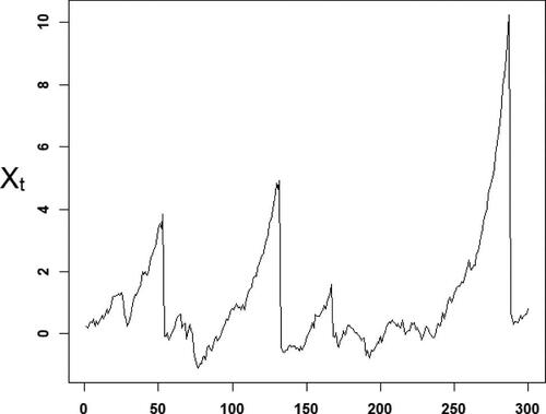
Dynamic models often admit solution processes for which the current value of the variable is a function of future values of an independent error process. Such solutions, called anticipative or noncausal, have attracted increasing attention in the financial and econometric literatures. In particular, noncausal processes have been found convenient for modeling locally explosive phenomena in financial time series such as speculative bubbles, while featuring heavy-tailed marginals and conditional heteroscedastic effects (Bec, Nielsen, and Saïdi 2020; Cavaliere, Nielsen, and Rahbek 2020; Fries and Zakoian 2019; Gouriéroux and Jasiak 2018; Gouriéroux and Zakoian 2017; Hecq and Sun 2019; Hecq, Lieb, and Telg 2016; Hecq, Telg, and Lieb 2017a,b; Hencic and Gouriéroux 2015; Chen, Choi, and Escanciano 2017; Lanne, Nyberg, and Saarinen 2012b; Lanne and Saikkonen 2011, 2013). Figure 1 depicts a typical simulated path of an elementary noncausal process, the α-stable noncausal AR(1), featuring multiple bubbles. In the framework of rational expectations price models (e.g., Diba and Grossman 1988a,b), prices $(P_t)$ are determined according to a model linking prices at date t and the present value of future prices and dividends $(D_t)$, say, $P_t={(1+r)}^{-1}{\mathbb{E}}_t[P_{t+1}+D_{t+1}]$, where r is, for simplicity, a constant real interest rate, and ${\mathbb{E}}_t$ is the expectation conditional on all information available at date t. The general solutions to such expectational difference equations are of the form $P_t=P_t^F+B_t$, where $P_t^F$ is a fundamental component—the discounted sum of expected future dividends—and $(B_t)$ is a bubble component which obeys $B_t={(1+r)}^{-1}{\mathbb{E}}_t[B_{t+1}]$ (Diba and Grossman 1988a,b), for example, the classical bubble model proposed by Blanchard and Watson (1982). In addition to capturing stylized facts of speculative episodes in financial time series, noncausal processes have also been shown to be suitable candidates for modeling the bubble component $(B_t)$ of prices in the framework of rational expectation price models (Gouriéroux, Jasiak, and Monfort 2020). Noncausal processes thus constitute an attractive family of models to capture the dynamics of speculative bubbles in financial time series data, forecast their future trajectories, and infer the odds of crashes. This would enable for instance risk managers to assess large downside risks during prolonged bull markets and the regulator to adjust requirements and restrictions to ensure resilience of the financial system.

Fig. 1 Sample path of an elementary bubble-generating noncausal process: the noncausal AR(1), strictly stationary solution of $X_t=\rho X_{t+1}+{\epsilon }_t,\rho =0.95$, with α-stable errors.

However, the limited knowledge about the predictive distribution of noncausal processes, especially during explosive bubble events, is impeding the ability to forecast them, thus limiting their use in practical applications. Taking notice of the absence of closed-form formulas for conditional moments and the predictive density except in special cases (see, e.g., Gouriéroux and Zakoian 2017, sec. 3.2; Fries and Zakoian 2019, sec. 3), two simulation- and sample-based methods have been proposed in the noncausal literature to approximate the conditional distribution of noncausal processes (Lanne, Luoto, and Saikkonen 2012a; Gouriéroux and Jasiak 2016). While offering flexible alternatives for forecasting noncausal processes beyond the special cases, Hecq and Voisin (2020) found that these methods can become computationally intense for larger prediction horizons and that accurately capturing the dynamics during explosive episodes may prove challenging (see also Gouriéroux, Hencic, and Jasiak 2019). Partial results have been obtained by Gouriéroux and Zakoian (2017) on the conditional moments of noncausal AR(1) processes driven by independent and identically distributed (iid) α-stable errors, which have been extended to mixed causal–noncausal AR processes with single ill-located root by Fries and Zakoian (2019). Despite stable noncausal processes featuring infinite marginal variance, their conditional moments may exist up to integer order four. In special cases, expressions of the conditional expectation and variance have been obtained, and revealed that noncausal processes can feature GARCH-type effects in calendar time despite such effects not being explicitly included in the modeling (Fries and Zakoian 2019). Provided the expressions of the conditional moments are derived, this suggests that point forecasts of noncausal processes based on their conditional expectation, variance, skewness and kurtosis could be formulated—as opposed to other predictors specifically introduced to circumvent the infinite variance of α-stable processes, such as minimum $L^{\alpha }$-dispersion or maximum covariation (see Karcher, Shmileva, and Spodarev 2013 and the references therein).

The aim of this article is to provide practical analytical results to compute the conditional moments of α-stable noncausal processes and to compute the crash odds of bubbles that such processes generate. First, the article extends the literature on the conditional moments $\mathbb{E}[X_2^p|X_1]$ of arbitrary bivariate α-stable random vectors (X₁, X₂) (Cioczek-Georges and Taqqu 1995a,b, 1998; Hardin, Samorodnitsky, and Taqqu 1991; Samorodnitsky and Taqqu 1994) by providing formulas for the orders p = 2, 3, 4. We then apply these results to derive a complete characterization of the conditional moments $\mathbb{E}[X_{t+h}^p|X_t],p=1,2,3,4,h\ge 1$, for $(X_t)$ an infinite two-sided moving average (MA) process driven by iid α-stable errors(1.1) $$X_t=\sum _{k\in \mathbb{Z}}{a}_k{\epsilon }_{t+k},$$(1.1) where $(a_k)$ is a nonrandom coefficients sequence satisfying mild conditions for $(X_t)$ to be well-defined and strictly stationary. Second, the conditional distribution of noncausal processes during explosive bubble episodes is analyzed. Provided the errors have probability tails similar to that of α-stable distributions, in the sense that they also feature power law tails, we obtain closed-form formulas valid during explosive episodes. These expressions provide illuminating interpretations on the dynamics of the bubbles that such models generate and a practical way to quantify the crash odds. Implications and parallels with the literature on rational expectation bubble models in the line of Blanchard and Watson (1982) are discussed.

The rest of the article is organized as follows. Section 2 recalls properties of bivariate stable distributions and provides our results on the conditional moments up to order four of arbitrary bivariate α-stable vectors. Applying these results to models of the form Equation (1.1)(1.1) $$X_t=\sum _{k\in \mathbb{Z}}{a}_k{\epsilon }_{t+k},$$(1.1) , Section 3 proposes a sufficient condition on the coefficients $(a_k)$ for the existence of conditional moments, characterizes their expressions when they exist, and discusses several examples and methodological aspects. Section 4 derives closed-form formulas for the predictive distribution of noncausal processes during explosive bubble episodes. Proofs and complementary results are collected in a supplementary file.

2 Conditional Moments of Bivariate α-Stable Vectors

We begin by recalling some properties of bivariate stable vectors (X₁, X₂) and then propose new expressions for their higher-order conditional power moments $\mathbb{E}[X_2^p|X_1]$. These expressions will apply to $(X_t,X_{t+h})$ when considering α-stable noncausal processes in the next section. The proof of the main results of this section draw upon the techniques used in Theorems 5.2.2–5.2.3 and Corollary 5.2.5 in Samorodnitsky and Taqqu (1994).

Letting $\alpha \in (0,2)$, a random vector $\mathit{X}=(X_1,X_2)$ is said to be an α-stable random vector in ${\mathbb{R}}^2$ (see in Samorodnitsky and Taqqu 1994, theor. 2.3.1) if there exists a unique pair $(\Gamma ,{\mathit{\mu }}^0)$, where Γ is a finite measure on the Euclidean unit sphere S₂ and ${\mathit{\mu }}^0$ a vector in ${\mathbb{R}}^2$, such that, for any $\mathit{u}\in {\mathbb{R}}^2$, the characteristic function of X writes(2.1) $$\begin{array}{c}\mathbb{E}\left[e^{i〈\mathit{u},\mathit{X}〉}\right]=\hspace{0.17em}\text{exp}\hspace{0.17em}\{\mathrm{}-\mathrm{}{\int }_{S_2}\mathrm{}|〈\mathit{u},\mathit{s}〉{|}^{\alpha }\\ \hspace{1em}(1-i \text{sign}(〈\mathit{u},\mathit{s}〉)w(\alpha ,〈\mathit{u},\mathit{s}〉)\mathrm{})\Gamma (d\mathit{s})+i 〈\mathit{u},{\mathit{\mu }}^0〉\},\end{array}$$(2.1) where $〈·,·〉$ is the canonical inner product, $w(\alpha ,s)=\text{tg}\left(\frac{\pi \alpha }{2}\right)$, if $\alpha \ne 1$, and $w(1,s)=-\frac{2}{\pi }\text{ln}\hspace{0.17em}\left|s\right|$ otherwise, for $s\in \mathbb{R}$. The measure Γ and the vector ${\mathit{\mu }}^0$ are, respectively, called the spectral measure and the shift vector of X. The pair $(\Gamma ,{\mathit{\mu }}^0)$ is said to be the spectral representation of X. The spectral measure Γ of a stable vector X in particular completely characterizes the tail dependence between its components: it holds that $\mathbb{P}(\mathit{X}/|\left|\mathit{X}\right||\in A | \left|\right|\mathit{X}\left|\right|>x)\to \Gamma (A)/\Gamma (S_2)$ as $x\to +\infty$, for any continuity set $A\subset S_2$ (Samorodnitsky and Taqqu 1994, theor. 4.4.8), where $\left|\right|·\left|\right|$ denotes the Euclidean norm. Intuitively, the more mass Γ attributes to some points of the unit sphere S₂, the more likely (X₁, X₂) is to be colinear to these points when it is large in norm. The counterpart of Equation (2.1)(2.1) $$\begin{array}{c}\mathbb{E}\left[e^{i〈\mathit{u},\mathit{X}〉}\right]=\hspace{0.17em}\text{exp}\hspace{0.17em}\{\mathrm{}-\mathrm{}{\int }_{S_2}\mathrm{}|〈\mathit{u},\mathit{s}〉{|}^{\alpha }\\ \hspace{1em}(1-i \text{sign}(〈\mathit{u},\mathit{s}〉)w(\alpha ,〈\mathit{u},\mathit{s}〉)\mathrm{})\Gamma (d\mathit{s})+i 〈\mathit{u},{\mathit{\mu }}^0〉\},\end{array}$$(2.1) for a univariate α-stable variable reads $\mathbb{E}[e^{\mathit{iuX}}]=\hspace{0.17em}\text{exp}\hspace{0.17em}\{-{\sigma }^{\alpha }|u{|}^{\alpha }(1-i\beta \text{sign}(u)w(\alpha ,u))+iu\mu \}$, for some asymmetry $\beta \in [-1,1]$, scale $\sigma >0$ and location $\mu \in \mathbb{R}$.

Stable distributions are known to have very few marginal moments. However, the distribution of one component of vector (X₁, X₂) conditionally on the other can have more moments according to the degree of dependence between them. If the spectral measure Γ of an α-stable random vector $\mathit{X}=(X_1,X_2)$ satisfies(2.2) $${\int }_{S_2}|s_1{|}^{-\nu }\Gamma (ds)<+\infty ,\hspace{1em}\text{for}\mathrm{ }\text{some}\hspace{1em}\nu \ge 0,$$(2.2) then, $\mathbb{E}[|X_2{|}^{\gamma }|X_1=x]<+\infty$ for almost every x if $0\le \gamma <\min (\alpha +\nu ,2\alpha +1)<5$ (see Samorodnitsky and Taqqu 1994, theor. 5.1.3 for details), entailing that conditional moments up to integer order four may exist although $\mathbb{E}[|X_2{|}^{\alpha }]=+\infty$. The conditional expectation of arbitrary α-stable bivariate vectors has been studied in details and its expression is recalled in Theorem 2.1, while the conditional variance received attention most exclusively in the symmetric α-Stable case.

We provide and prove new formulas for the conditional power moments of order 2, 3, and 4 of arbitrary (not necessarily symmetric) α-stable bivariate vectors (X₁, X₂). The second-order moment in the case α = 1, which requires special treatment when not restricting to symmetric stable distributions, is also considered. In the rest of this section, we assume without loss of generality that the shift vector ${\mathit{\mu }}^0=({\mu }_1^0,{\mu }_2^0)$ is zero. This can be done without loss of generality because, assuming the conditional moment of order p exists, $\mathbb{E}[X_2^p|X_1=x]=\mathbb{E}[{(X_2-{\mu }_2^0+{\mu }_2^0)}^p|X_1-{\mu }_1^0=x-{\mu }_1^0]={\sum }_{j=0}^p{\mathrm{C}}_p^j{({\mu }_2^0)}^{p-j}\mathbb{E}[{\tilde{X}}_2^j|{\tilde{X}}_1=\tilde{x}]$ where ${\mathrm{C}}_p^j$ is the binomial coefficient, $\tilde{x}=x-{\mu }_1^0$, and $({\tilde{X}}_1,{\tilde{X}}_2)=(X_1-{\mu }_1^0,X_2-{\mu }_2^0)$ has the same spectral measure as (X₁, X₂) and zero shift parameter. We first consider the case $\alpha \ne 1$ and introduce useful constants and functions which generalize existing quantities in the literature. For $p\in \{1,2,3,4\}$, when they exist, define(2.3) $$\begin{array}{c}{\sigma }_1^{\alpha }={\int }_{S_2}|s_1{|}^{\alpha }\Gamma (d\mathit{s}),{\beta }_1=\frac{{\int }_{S_2}{s}_1^{<\alpha >}\Gamma (d\mathit{s})}{{\sigma }_1^{\alpha }},\\ {\kappa }_p=\frac{{\int }_{S_2}{(\frac{s_2}{s_1})}^p|s_1{|}^{\alpha }\Gamma (d\mathit{s})}{{\sigma }_1^{\alpha }},{\lambda }_p=\frac{{\int }_{S_2}{(\frac{s_2}{s_1})}^p{s}_1^{<\alpha >}\Gamma (d\mathit{s})}{{\sigma }_1^{\alpha }},\mathrm{\hspace{1em}}\mathrm{\hspace{1em}}\end{array}$$(2.3) where $y^{<r>}=\text{sign}(y)|y{|}^r$ for any $y,r\in \mathbb{R}$. For any $n\in \mathbb{N},\mathit{\theta }=({\theta }_1,{\theta }_2)\in {\mathbb{R}}^2,x\in \mathbb{R}$, define $\mathcal{H}$ as(2.4) $$\begin{array}{c}\mathcal{H}(n,\mathit{\theta };x)={\int }_0^{+\infty }{e}^{-{\sigma }_1^{\alpha }{u}^{\alpha }}{u}^{n(\alpha -1)}({\theta }_1\hspace{0.17em}\text{cos}\hspace{0.17em}(ux-a{\beta }_1{\sigma }_1^{\alpha }{u}^{\alpha })\\ +{\theta }_2\hspace{0.17em}\text{sin}\hspace{0.17em}(ux-a{\beta }_1{\sigma }_1^{\alpha }{u}^{\alpha }))du.\end{array}$$(2.4)

The new family of functions $\mathcal{H}$ introduced contains functions related to the marginal density of the stable random variable $X_1\sim \mathcal{S}(\alpha ,{\beta }_1,{\sigma }_1,0),\alpha \ne 1$: $f_{X_1}(x):=\frac{1}{\pi }\mathcal{H}(0,(1,0);x)=\frac{1}{\pi }{\int }_0^{+\infty }{e}^{-{\sigma }_1^{\alpha }{u}^{\alpha }}\hspace{0.17em}\text{cos}\hspace{0.17em}(ux-a{\beta }_1{\sigma }_1^{\alpha }{u}^{\alpha })du$. The quantities σ₁ and β₁ denote the scale and asymmetry parameters of the marginal distribution of X₁, whereas the constants κ_p ’s and λ_p ’s generalize standard dependence measures invoked in the literature. Noticeably, ${\kappa }_1={\int }_{S_2}{s}_2{s}_1^{<\alpha -1>}\Gamma (d\mathit{s})/{\sigma }_1^{\alpha }$ corresponds to the normalized covariation between X₂ and X₁. This dependence measure was been introduced by Miller (1978) and Cambanis and Miller (1981) to replace the ill-defined covariance between two symmetric α-stable random variables, and has been a popular tool to formulate point forecasts of infinite variance α-stable processes [see Karcher, Shmileva, and Spodarev (2013) and the references therein]. The new constants κ_p and λ_p , $p\ge 2$ introduced here, which intervene in the expressions of the higher order conditional moments of (X₁, X₂), can be seen as extending this dependence measure to higher powers of X₁ and X₂ in the asymmetric case. The following result recalls the expression of the conditional expectation in the case $\alpha \ne 1$.

Theorem 2.1

(Theorem 5.2.2, Samorodnitsky and Taqqu 1994). Let (X₁, X₂) be an α-stable random vector with spectral representation $(\Gamma ,\mathit{0})$. For $\alpha \in (0,2)\setminus \left\{1\right\}$ and letting Γ satisfy Equaiton (2.2) with $\nu >1-\alpha$ if $\alpha \in (0,1)$,(2.5) $$\mathbb{E}\left[X_2\right|X_1=x]={\kappa }_{1}x+\frac{a({\lambda }_1-{\beta }_1{\kappa }_1)}{1+a^2{\beta }_1^2}[a{\beta }_{1}x+\frac{1-xH(x)}{\pi f_{X_1}(x)}],$$(2.5) where $a=\text{tg}(\pi \alpha /2)$, β₁, κ₁ and λ₁ are as in Equation (2.3)(2.3) $$\begin{array}{c}{\sigma }_1^{\alpha }={\int }_{S_2}|s_1{|}^{\alpha }\Gamma (d\mathit{s}),{\beta }_1=\frac{{\int }_{S_2}{s}_1^{<\alpha >}\Gamma (d\mathit{s})}{{\sigma }_1^{\alpha }},\\ {\kappa }_p=\frac{{\int }_{S_2}{(\frac{s_2}{s_1})}^p|s_1{|}^{\alpha }\Gamma (d\mathit{s})}{{\sigma }_1^{\alpha }},{\lambda }_p=\frac{{\int }_{S_2}{(\frac{s_2}{s_1})}^p{s}_1^{<\alpha >}\Gamma (d\mathit{s})}{{\sigma }_1^{\alpha }},\mathrm{\hspace{1em}}\mathrm{\hspace{1em}}\end{array}$$(2.3) and $H( · ):=\mathcal{H}(0,(0,1); · )$.

We now state our result in the case $\alpha \ne 1$ for the conditional moments of order two, three and four.

Theorem 2.2.

Let (X₁, X₂) be an α-stable random vector with spectral representation $(\Gamma ,\mathit{0})$.

For $\alpha \in (1/2,2)\setminus \left\{1\right\}$ and Γ satisfying (2.2) with $\nu >2-\alpha$,(2.6) $$\begin{array}{c}\mathbb{E}\left[X_2^2\right|X_1=x]={\kappa }_2{x}^2+\frac{ax({\lambda }_2-{\beta }_1{\kappa }_2)}{1+{(a{\beta }_1)}^2}[a{\beta }_{1}x+\frac{1-xH(x)}{\pi f_{X_1}(x)}]\\ - \frac{{\alpha }^2{\sigma }_1^{2\alpha }}{\pi f_{X_1}(x)}\mathcal{H}(2,{\mathit{\theta }}_1;x).\end{array}$$(2.6)

For $\alpha \in (1,2)$ and Γ satisfying Equation (2.2)(2.2) $${\int }_{S_2}|s_1{|}^{-\nu }\Gamma (ds)<+\infty ,\hspace{1em}\text{for}\mathrm{ }\text{some}\hspace{1em}\nu \ge 0,$$(2.2) with $\nu >3-\alpha$,(2.7) $$\begin{array}{c}\mathbb{E}\left[X_2^3\right|X_1=x]={\kappa }_3{x}^3+\frac{a{x}^2({\lambda }_3-{\beta }_1{\kappa }_3)}{1+{(a{\beta }_1)}^2}[a{\beta }_{1}x+\frac{1-xH(x)}{\pi f_{X_1}(x)}]\\ - \frac{{\alpha }^2{\sigma }_1^{2\alpha }}{2\pi f_{X_1}(x)}[x\mathcal{H}(2,{\mathit{\theta }}_2;x)+\alpha {\sigma }_1^{\alpha }\mathcal{H}(3,{\mathit{\theta }}_3;x)].\end{array}$$(2.7)

For $\alpha \in (3/2,2)$ and Γ satisfying Equation (2.2)(2.2) $${\int }_{S_2}|s_1{|}^{-\nu }\Gamma (ds)<+\infty ,\hspace{1em}\text{for}\mathrm{ }\text{some}\hspace{1em}\nu \ge 0,$$(2.2) with $\nu >4-\alpha$,(2.8) $$\begin{array}{c}\mathbb{E}\left[X_2^4\right|X_1=x]={\kappa }_4{x}^4+\frac{a{x}^3({\lambda }_4-{\beta }_1{\kappa }_4)}{1+{(a{\beta }_1)}^2}\\ \times [a{\beta }_{1}x+\frac{1-xH(x)}{\pi f_{X_1}(x)}]-\frac{{\alpha }^2{\sigma }_1^{2\alpha }}{\pi f_{X_1}(x)}\\ \times [\frac{x^2}{2}\mathcal{H}(2,{\mathit{\theta }}_4;x)+\frac{\alpha x{\sigma }_1^{\alpha }}{6}\mathcal{H}(3,{\mathit{\theta }}_5;x)\\ + \frac{{\alpha }^2{\sigma }_1^{2\alpha }}{3}\mathcal{H}(4,{\mathit{\theta }}_6;x)].\end{array}$$(2.8)

Here, $a=\text{tg} (\pi \alpha /2)$, $H( · )=\mathcal{H}(0,(0,1); · ),{\mathit{\theta }}_1=({\theta }_{11},{\theta }_{12})$ in Equation (2.6)(2.6) $$\begin{array}{c}\mathbb{E}\left[X_2^2\right|X_1=x]={\kappa }_2{x}^2+\frac{ax({\lambda }_2-{\beta }_1{\kappa }_2)}{1+{(a{\beta }_1)}^2}[a{\beta }_{1}x+\frac{1-xH(x)}{\pi f_{X_1}(x)}]\\ - \frac{{\alpha }^2{\sigma }_1^{2\alpha }}{\pi f_{X_1}(x)}\mathcal{H}(2,{\mathit{\theta }}_1;x).\end{array}$$(2.6) is given by$$\begin{array}{c}{\theta }_{11}={\kappa }_1^2-a^2{\lambda }_1^2+a^2{\beta }_1{\lambda }_2-{\kappa }_2,\\ {\theta }_{12}=a({\lambda }_2+{\beta }_1{\kappa }_2)-2a{\lambda }_1{\kappa }_1,\end{array}$$and the remaining ${\mathit{\theta }}_i$’s in Equations (2.7)(2.7) $$\begin{array}{c}\mathbb{E}\left[X_2^3\right|X_1=x]={\kappa }_3{x}^3+\frac{a{x}^2({\lambda }_3-{\beta }_1{\kappa }_3)}{1+{(a{\beta }_1)}^2}[a{\beta }_{1}x+\frac{1-xH(x)}{\pi f_{X_1}(x)}]\\ - \frac{{\alpha }^2{\sigma }_1^{2\alpha }}{2\pi f_{X_1}(x)}[x\mathcal{H}(2,{\mathit{\theta }}_2;x)+\alpha {\sigma }_1^{\alpha }\mathcal{H}(3,{\mathit{\theta }}_3;x)].\end{array}$$(2.7) and (2.8)(2.8) $$\begin{array}{c}\mathbb{E}\left[X_2^4\right|X_1=x]={\kappa }_4{x}^4+\frac{a{x}^3({\lambda }_4-{\beta }_1{\kappa }_4)}{1+{(a{\beta }_1)}^2}\\ \times [a{\beta }_{1}x+\frac{1-xH(x)}{\pi f_{X_1}(x)}]-\frac{{\alpha }^2{\sigma }_1^{2\alpha }}{\pi f_{X_1}(x)}\\ \times [\frac{x^2}{2}\mathcal{H}(2,{\mathit{\theta }}_4;x)+\frac{\alpha x{\sigma }_1^{\alpha }}{6}\mathcal{H}(3,{\mathit{\theta }}_5;x)\\ + \frac{{\alpha }^2{\sigma }_1^{2\alpha }}{3}\mathcal{H}(4,{\mathit{\theta }}_6;x)].\end{array}$$(2.8) , which depend only on α, β₁, and the κ_p ’s and λ_p ’s in Equation (2.3)(2.3) $$\begin{array}{c}{\sigma }_1^{\alpha }={\int }_{S_2}|s_1{|}^{\alpha }\Gamma (d\mathit{s}),{\beta }_1=\frac{{\int }_{S_2}{s}_1^{<\alpha >}\Gamma (d\mathit{s})}{{\sigma }_1^{\alpha }},\\ {\kappa }_p=\frac{{\int }_{S_2}{(\frac{s_2}{s_1})}^p|s_1{|}^{\alpha }\Gamma (d\mathit{s})}{{\sigma }_1^{\alpha }},{\lambda }_p=\frac{{\int }_{S_2}{(\frac{s_2}{s_1})}^p{s}_1^{<\alpha >}\Gamma (d\mathit{s})}{{\sigma }_1^{\alpha }},\mathrm{\hspace{1em}}\mathrm{\hspace{1em}}\end{array}$$(2.3) , are given in (D.1)–(D.10) in the supplementary file.

Proof.

See Sections B, C, and D in the supplementary file.

Let us now turn to the case α = 1, which encompasses in particular the case of Cauchy marginals. The following result recalls the expression of the conditional expectation in this case.

Theorem 2.3

(Theorem 5.2.3, Samorodnitsky and Taqqu 1994). Let (X₁, X₂) be α-stable, with α = 1 and spectral representation $(\Gamma ,\mathit{0})$, where Γ satisfies (2.2) with $\nu >0$. Then, for almost every x,$$\begin{array}{c}\mathbb{E}\left[X_2\right|X_1=x]=-a{\sigma }_1{q}_0+{\kappa }_1(x-{\mu }_1)+\frac{{\lambda }_1-{\beta }_1{\kappa }_1}{{\beta }_1}\\ \times [(x-{\mu }_1)-{\sigma }_1\frac{U(x)}{\pi f_{X_1}(x)}],\end{array}$$if ${\beta }_1\ne 0$, and$$\mathbb{E}\left[X_2\right|X_1=x]=-a{\sigma }_1{q}_0+{\kappa }_1(x-{\mu }_1)-a{\sigma }_1{\lambda }_1\frac{V(x)}{\pi f_{X_1}(x)},$$ if ${\beta }_1=0$. Here, $a=2/\pi$, σ₁, β₁, κ₁ and λ₁ are as in Equation (2.3)(2.3) $$\begin{array}{c}{\sigma }_1^{\alpha }={\int }_{S_2}|s_1{|}^{\alpha }\Gamma (d\mathit{s}),{\beta }_1=\frac{{\int }_{S_2}{s}_1^{<\alpha >}\Gamma (d\mathit{s})}{{\sigma }_1^{\alpha }},\\ {\kappa }_p=\frac{{\int }_{S_2}{(\frac{s_2}{s_1})}^p|s_1{|}^{\alpha }\Gamma (d\mathit{s})}{{\sigma }_1^{\alpha }},{\lambda }_p=\frac{{\int }_{S_2}{(\frac{s_2}{s_1})}^p{s}_1^{<\alpha >}\Gamma (d\mathit{s})}{{\sigma }_1^{\alpha }},\mathrm{\hspace{1em}}\mathrm{\hspace{1em}}\end{array}$$(2.3) , $f_{X_1}$ is the marginal density of $X_1\sim \mathcal{S}(1,{\beta }_1,{\sigma }_1,{\mu }_1),q_0=\frac{1}{{\sigma }_1}{\int }_{S_2}{s}_2\hspace{0.17em}\text{ln}\hspace{0.17em}\left|s_1\right|\Gamma (d\mathit{s}),{\mu }_1=-a{\int }_{S_2}{s}_1\hspace{0.17em}\text{ln}\hspace{0.17em}\left|s_1\right|\Gamma (d\mathit{s})$, and U, V are given in (E.12)–(E.13) in the supplementary file.

We next provide our result for the second-order conditional moment when α = 1. As for the conditional expectation, two different expressions hold according to whether the marginal distribution of X₁ is skewed or symmetric.

Theorem 2.4.

Let (X₁, X₂) be α-stable, with α = 1 and spectral representation $(\Gamma ,\mathit{0})$, where Γ satisfies Equation (2.2)(2.2) $${\int }_{S_2}|s_1{|}^{-\nu }\Gamma (ds)<+\infty ,\hspace{1em}\text{for}\mathrm{ }\text{some}\hspace{1em}\nu \ge 0,$$(2.2) with $\nu >1$. Then, for almost every x,$$\begin{array}{c}\mathbb{E}\left[X_2^2\right|X_1=x]={\sigma }_1^2(a^2{q}_0^2-{\kappa }_1^2)+\frac{2{\sigma }_1{\lambda }_1}{{\beta }_1}({\sigma }_1{\kappa }_1-a{q}_0(x-{\mu }_1))\\ +\frac{{\lambda }_2}{{\beta }_1}({(x-{\mu }_1)}^2-{\sigma }_1^2)\\ +(a{\sigma }_1{q}_0({\lambda }_1-{\beta }_1{\kappa }_1)+({\kappa }_1{\lambda }_1-{\lambda }_2)(x-{\mu }_1))\\ \times \frac{2{\sigma }_{1}U(x)}{{\beta }_1\pi f_{X_1}(x)}+({\lambda }_2+{\beta }_1{\kappa }_2-2{\kappa }_1{\lambda }_1\\ + a^2{\sigma }_1{\beta }_1({\lambda }_1^2-{\beta }_1{\lambda }_2)W(x))\frac{{\sigma }_1}{{\beta }_1\pi f_{X_1}(x)},\end{array}$$if ${\beta }_1\ne 0$, and$$\begin{array}{c}\mathbb{E}\left[X_2^2\right|X_1=x]\\ \mathrm{\hspace{1em}}\mathrm{\hspace{1em}}={\sigma }_1^2({\kappa }_2+a^2{q}_0^2-{\kappa }_1^2)-2a{\sigma }_1{\kappa }_1{q}_0(x-{\mu }_1)\\ \mathrm{\hspace{1em}}\mathrm{\hspace{1em}}\hspace{1em}+ {\kappa }_2{(x-{\mu }_1)}^2+a{\sigma }_1({\lambda }_2-2{\lambda }_1{\kappa }_1)\frac{F_{X_1}(x)-1/2}{f_{X_1}(x)}\\ \mathrm{\hspace{1em}}\mathrm{\hspace{1em}}\hspace{1em}+ \frac{a{\sigma }_1{\lambda }_1}{\pi f_{X_1}(x)}[2(a{\sigma }_1{q}_0-{\kappa }_1(x-{\mu }_1))V(x)+a{\sigma }_1{\lambda }_{1}W(x)],\end{array}$$ if ${\beta }_1=0$. Here, $a=2/\pi$, σ₁, β₁, the κ_p ’s and the λ_p ’s are as in Equation (2.3)(2.3) $$\begin{array}{c}{\sigma }_1^{\alpha }={\int }_{S_2}|s_1{|}^{\alpha }\Gamma (d\mathit{s}),{\beta }_1=\frac{{\int }_{S_2}{s}_1^{<\alpha >}\Gamma (d\mathit{s})}{{\sigma }_1^{\alpha }},\\ {\kappa }_p=\frac{{\int }_{S_2}{(\frac{s_2}{s_1})}^p|s_1{|}^{\alpha }\Gamma (d\mathit{s})}{{\sigma }_1^{\alpha }},{\lambda }_p=\frac{{\int }_{S_2}{(\frac{s_2}{s_1})}^p{s}_1^{<\alpha >}\Gamma (d\mathit{s})}{{\sigma }_1^{\alpha }},\mathrm{\hspace{1em}}\mathrm{\hspace{1em}}\end{array}$$(2.3) , $f_{X_1}$ and $F_{X_1}$ are, respectively, the marginal density and cumulative distribution function of $X_1\sim \mathcal{S}(1,{\beta }_1,{\sigma }_1,{\mu }_1),q_0=\frac{1}{{\sigma }_1}{\int }_{S_2}{s}_2\hspace{0.17em}\text{ln}\hspace{0.17em}\left|s_1\right|\Gamma (d\mathit{s}),{\mu }_1=-a{\int }_{S_2}{s}_1\hspace{0.17em}\text{ln}\hspace{0.17em}\left|s_1\right|\Gamma (d\mathit{s})$, and U, V, and W are given in (E.12)–(E.14) in the supplementary file.

Proof.

See Section E in the supplementary file.

The expressions of the conditional moments simplify when one considers the asymptotics with respect to the conditioning variable, as $X_1=x$ becomes large.

Proposition 2.1.

Let $p\in \{1,2,3,4\}$ and let (X₁, X₂) be α-stable with $\alpha \in (0,2)$, and spectral representation $(\Gamma ,\mathit{0})$ such that the conditional moment of order p exists. If $\left|{\beta }_1\right|\ne 1$, then$$\begin{array}{c}{x}^{-p} \mathbb{E}\left[X_2^p\right|X_1=x]\underset{x\to +\infty }{\to }\frac{{\kappa }_p+{\lambda }_p}{1+{\beta }_1},\\ x^{-p} \mathbb{E}\left[X_2^p\right|X_1=x]\underset{x\to -\infty }{\to }\frac{{\kappa }_p-{\lambda }_p}{1-{\beta }_1},\end{array}$$and if $\left|{\beta }_1\right|=1$ and ${\beta }_{1}x\to +\infty$, then, $x^{-p} \mathbb{E}[X_2^p|X_1=x]\to {\kappa }_p$.

Proof.

See Section F in the supplementary file.

The conditional moment of order p is thus asymptotically equivalent to x^p up to a multiplicative constant as $x\to \pm \infty$, except if either ${\kappa }_p+{\lambda }_p=0$ or ${\kappa }_p-{\lambda }_p=0$, in which case the conditional moment for the corresponding tail does not grow as fast as $|x{|}^p$ in absolute value.

Having provided the analytical formulas of the conditional moments for general stable bivariate vectors, we are now in the position to study the conditional moments of stable processes.

3 Conditional Moments of Noncausal α-Stable Processes

Operating the set of properties of bivariate α-stable distributions provided in the previous section, we study the existence and expressions of the conditional moments of α-stable infinite MA processes. Discussions on practical aspects as well as examples focusing on modeling practices of the empirical noncausal literature follow the main result.

Let us consider $(X_t)$ a two-sided MA($\infty$) process as in Equation (1.1)(1.1) $$X_t=\sum _{k\in \mathbb{Z}}{a}_k{\epsilon }_{t+k},$$(1.1) with α-stable errors ${\epsilon }_t\stackrel{\text{iid}}{\sim }\mathcal{S}(\alpha ,\beta ,\sigma ,\mu )$ and coefficients $(a_k)$ satisfying(3.1) $$\sum _{k\in \mathbb{Z}}|a_k{|}^s<+\infty ,\mathrm{ }\text{for}\mathrm{ }\text{some}\mathrm{ }s\in (0,\alpha )\cap [0,1],$$(3.1) (3.2) $$\mathrm{ }\text{and}\mathrm{ }\text{in}\mathrm{ }\text{addition}\mathrm{ }\text{for}\mathrm{ }\alpha =1,\beta \ne 0,\sum _{k\in \mathbb{Z}}\left|a_k\right||\mathrm{}\hspace{0.17em}\text{ln}\hspace{0.17em}|a_k\left|\right|<+\infty .$$(3.2)

Conditions (3.1) and (3.2) ensure that $\sum _{k\in \mathbb{Z}}{a}_k{\epsilon }_{t+k}$ converges absolutely almost surely so that $(X_t)$ is well defined and strictly stationary. An MA process of the form Equation (1.1)(1.1) $$X_t=\sum _{k\in \mathbb{Z}}{a}_k{\epsilon }_{t+k},$$(1.1) satisfying the above conditions is said to be purely causal if a_k = 0 for k > 0 and purely noncausal if a_k = 0 for k < 0. Noncausality is found to be crucial for the existence of conditional moments higher than order α. An important class of models that we shall consider and which admits MA($\infty$) representations satisfying the above conditions is the class of ARMA processes. General mixed ARMA processes (MARMA)—causal, noncausal, invertible, or noninvertible—are strictly stationary solutions of stochastic recursive equations of the form(3.3) $$\psi (F)\varphi (B)X_t=\Theta (F)H(B){\epsilon }_t,$$(3.3) where F (resp. $B=F^{-1}$) denotes the forward (resp. backward) operator, $\psi (z):=1-{\psi }_{1}z-\cdots -{\psi }_p{z}^p$ and $\varphi (z):=1-{\varphi }_{1}z-\cdots -{\varphi }_q{z}^q$ are polynomials of degrees p and q, and Θ and H are two polynomials of respective degrees r and s with roots on or outside the unit circle. Equation (3.3)(3.3) $$\psi (F)\varphi (B)X_t=\Theta (F)H(B){\epsilon }_t,$$(3.3) admits a unique strictly stationary solution, called a MARMA($p,q,r,s$), provided that $\psi (z)\ne 0,\varphi (z)\ne 0$ for $\left|z\right|\le 1$, and that ψ (resp. $\varphi$) has no common root with Θ (resp. H). The stationary solution is noncausal if $p\ge 1$. When $\Theta =H=1,(X_t)$ reduces to a mixed causal–noncausal autoregressive process, denoted MAR(p, q).

3.1 Spectral Representation of $(X_t,X_{t+h})$

Because the error sequence $({\epsilon }_t)$ is α-stable distributed, the bivariate vector $(X_t,X_{t+h})$, for $(X_t)$ satisfying Equations (1.1)(1.1) $$X_t=\sum _{k\in \mathbb{Z}}{a}_k{\epsilon }_{t+k},$$(1.1) , (3.1)(3.1) $$\sum _{k\in \mathbb{Z}}|a_k{|}^s<+\infty ,\mathrm{ }\text{for}\mathrm{ }\text{some}\mathrm{ }s\in (0,\alpha )\cap [0,1],$$(3.1) , and (3.2), is itself α-stable for any horizon h and the results from the previous section apply. This is a consequence of the following lemma, which provides the spectral representation of discrete time vectors of linear MAs driven by α-stable iid errors.

Lemma 3.1.

Let $0<\alpha <2$. For ${\epsilon }_t\stackrel{\text{iid}}{\sim }\mathcal{S}(\alpha ,\beta ,\sigma ,\mu )$ and real deterministic sequences ${(a_{k,i})}_k$, i = 1, 2, both satisfying Equations (3.1)(3.1) $$\sum _{k\in \mathbb{Z}}|a_k{|}^s<+\infty ,\mathrm{ }\text{for}\mathrm{ }\text{some}\mathrm{ }s\in (0,\alpha )\cap [0,1],$$(3.1) and (3.2)(3.2) $$\mathrm{ }\text{and}\mathrm{ }\text{in}\mathrm{ }\text{addition}\mathrm{ }\text{for}\mathrm{ }\alpha =1,\beta \ne 0,\sum _{k\in \mathbb{Z}}\left|a_k\right||\mathrm{}\hspace{0.17em}\text{ln}\hspace{0.17em}|a_k\left|\right|<+\infty .$$(3.2) , let ${\mathit{X}}_{\mathit{t}}=(X_{1,t},X_{2,t})$, with $X_{i,t}=\sum _{k\in \mathbb{Z}}{a}_{k,i}{\epsilon }_{t+k}$, and denote ${\mathit{a}}_k=(a_{k,1},a_{k,2})$ for $k\in \mathbb{Z}$. Then, ${\mathit{X}}_{\mathit{t}}$ is an α-stable random vector in ${\mathbb{R}}^2$, with spectral representation $(\Gamma ,{\mathit{\mu }}^0)$ given by(3.4) $$\begin{array}{c}\Gamma (A)={\sigma }^{\alpha }\sum _{s=\pm 1}\sum _{k\in \mathbb{Z}}\frac{1+s\beta }{2}\left|\right|{\mathit{a}}_k|{|}^{\alpha }{\delta }_{\left\{\frac{s{\mathit{a}}_k}{\left|\right|{\mathit{a}}_k\left|\right|}\right\}}(A),\\ {\mathit{\mu }}^0=\sum _{k\in \mathbb{Z}}{\mathit{a}}_k\mu -\mathrm{ }{1}_{\{\alpha =1\}}\frac{2}{\pi }\sigma \beta \sum _{k\in \mathbb{Z}}{\mathit{a}}_k\hspace{0.17em}\text{ln}\hspace{0.17em}\left|\right|{\mathit{a}}_k\left|\right|,\end{array}$$(3.4) for any Borel set $A\subset S_2$, where ${\delta }_{\left\{\mathit{x}\right\}}(A)=1$ if $\mathit{x}\in A$, else ${\delta }_{\left\{\mathit{x}\right\}}(A)=0$, is the Dirac measure at point $\mathit{x}\in {\mathbb{R}}^2,\left|\right|·\left|\right|$ stands for the Euclidean norm, and by convention, if for some $k\in \mathbb{Z},{\mathit{a}}_k=\mathit{0}$, that is, $\left|\right|{\mathit{a}}_k\left|\right|=0$, then the k^th term vanishes from the sums.

Proof.

See Section G in the supplementary file.

3.2 Conditional Moments

The results on bivariate stable vectors immediately apply to ${\mathit{X}}_t=(X_t,X_{t+h})$ with ${\mathit{a}}_k=(a_k,a_{k-h})$. A sufficient condition for the existence of conditional moments is given in the following proposition as well as their expressions. Without loss of generality, we will assume in the rest of this section that the stable errors have zero location parameter, that is, μ = 0, unless stated otherwise.

Proposition 3.1.

Let $(X_t)$ be an α-stable two-sided MA($\infty$) process, $0<\alpha <2,\beta \in [-1,1],\sigma >0$, satisfying Equations (1.1)(1.1) $$X_t=\sum _{k\in \mathbb{Z}}{a}_k{\epsilon }_{t+k},$$(1.1) , (3.1)(3.1) $$\sum _{k\in \mathbb{Z}}|a_k{|}^s<+\infty ,\mathrm{ }\text{for}\mathrm{ }\text{some}\mathrm{ }s\in (0,\alpha )\cap [0,1],$$(3.1) , and (3.2) and let $h\ge 1$.

1. Assume there is $\nu \ge 0$ such that(3.5) $$\sum _{k\in \mathbb{Z}}(a_k^2+a_{k-h}^2{)}^{\frac{\alpha +\nu }{2}}|a_k{|}^{-\nu }<+\infty .$$(3.5)

   Then $\mathbb{E}[|X_{t+h}{|}^{\gamma }|X_t]<+\infty$ for $0\le \gamma <\min (\alpha +\nu ,2\alpha +1)$.

2. For $\alpha \ne 1$, the moments $\mathbb{E}[X_{t+h}^p|X_t],p\le 4$, when they exist, are given by Theorems 2.1 and 2.2 with$$\begin{array}{c}{\sigma }_1^{\alpha }={\sigma }^{\alpha }\sum _{k\in \mathbb{Z}}|a_k{|}^{\alpha },{\beta }_1=\beta \frac{\sum _{k\in \mathbb{Z}}{a}_k^{<\alpha >}}{\sum _{k\in \mathbb{Z}}|a_k{|}^{\alpha }},\\ {\kappa }_p=\frac{\sum _{k\in \mathbb{Z}}|a_k{|}^{\alpha }{\left(\frac{a_{k-h}}{a_k}\right)}^p}{\sum _{k\in \mathbb{Z}}|a_k{|}^{\alpha }},{\lambda }_p=\beta \frac{\sum _{k\in \mathbb{Z}}{a}_k^{<\alpha >}{\left(\frac{a_{k-h}}{a_k}\right)}^p}{\sum _{k\in \mathbb{Z}}|a_k{|}^{\alpha }}.\end{array}$$

3. For α = 1, let $({\tilde{X}}_t,{\tilde{X}}_{t+h}):=(X_t,X_{t+h})-{\mathit{\mu }}^0$ where ${\mathit{\mu }}^0$ is the shift vector as in Lemma 3.1. Then, the first- and second-order moments of ${\tilde{X}}_{t+h}|{\tilde{X}}_t$ are, respectively, given by Theorems 2.3 and 2.4 with the κ_p ’s, λ_p ’s, σ₁, β₁ as in $\iota \iota )$ and$$\begin{array}{c}{q}_0=\beta \sum _{k\in \mathbb{Z}}{a}_{k-h}\hspace{0.17em}\text{ln}\hspace{0.17em}\left(\frac{\left|a_k\right|}{\sqrt{a_k^2+a_{k-h}^2}}\right)/\sum _{k\in \mathbb{Z}}\left|a_k\right|,\\ {\mu }_1=-\frac{2\sigma \beta }{\pi }\sum _{k\in \mathbb{Z}}{a}_k\hspace{0.17em}\text{ln}\hspace{0.17em}\left(\frac{\left|a_k\right|}{\sqrt{a_k^2+a_{k-h}^2}}\right).\end{array}$$

By convention, in all the points above, if $(a_k,a_{k-h})=(0,0)$, then the kth term vanishes from the sums.

Remark 3.1

(Existence of moments). Point $\iota )$ provides a sufficient condition for the existence of conditional moments. Notice that the left-hand side of condition (3.5) is an increasing function of ν. Thus, if condition (3.5) holds for some ${\nu }_0>0$, it then holds for any $0\le \nu \le {\nu }_0$, and if it fails for ν₀, it then fails for all $\nu \ge {\nu }_0$. Causal processes, say of the form $\sum _{k\le 0}{a}_k{\epsilon }_{t+k}$ with $a_0=1$, automatically fail condition (3.5) for all $\nu >0$, as $(a_h,a_0)=(0,1)$ and the hth term of the sum is finite only if ν = 0. In the case of symmetric errors (β = 0), Theorem 1.1 by Cioczek-Georges and Taqqu (1995b) allows to conclude that condition (3.5) is also necessary and hence that causal processes do not have finite conditional moments for orders higher than α. Conversely, condition (3.5) may hold for some $\nu >0$ for noncausal processes provided the coefficients $(a_k)$ do not decay too fast as $k\to +\infty$. In fact, the slower the decay of $(a_k)$ as $k\to +\infty$, the higher the values of ν for which condition (3.5) will hold. In other terms, the stronger the dependence on ¡¡future¿¿ errors, the higher the order at which conditional moments will exist: hence the intuition that higher-order conditional moments may exist provided that the process is anticipative or noncausal enough. It is easy to show that condition (3.5) holds for any $\nu \ge 0$ as soon as $(a_k)$ decays geometrically or hyperbolically, guaranteeing the existence of conditional moments up to order $2\alpha +1$ at all prediction horizons for noncausal ARMA and fractionally integrated processes. Consider for instance a noncausal process $(X_t)$ of the form condition (1.1) such that a_k = 0 for k < 0, $a_k\ne 0$ for $k\ge 0$ and $a_k\underset{k\to +\infty }{\sim }c{\lambda }^k$, for some nonzero constant c and $\lambda \in (-1,1)$. Letting $\nu \ge 0$,$$\begin{array}{c}{(a_k^2+a_{k-h}^2)}^{\frac{\alpha +\nu }{2}}|a_k{|}^{-\nu }=|a_k{|}^{\alpha }{(1+\frac{a_{k-h}^2}{a_k^2})}^{\frac{\alpha +\nu }{2}}\\ \underset{k\to +\infty }{\sim }\left|c{|}^{\alpha }{(1+{\lambda }^{-2h})}^{\frac{\alpha +\nu }{2}}\right|\lambda {|}^{\alpha k},\end{array}$$and since $|\lambda {|}^{\alpha }<1$, the summability condition (3.5) holds for any $\nu \ge 0$. In particular, it holds for $\nu =\alpha +1$ and therefore, Point ι of Proposition 3.1 ensures that $(X_t)$ admits finite conditional moments up to order $2\alpha +1$. It is possible to find noncausal processes for which condition (3.5) holds only up to some $\nu \in [0,\alpha +1)$, that is, entailing that conditional moments are finite only up to order γ strictly within $(\alpha ,2\alpha +1)$, with γ moreover depending on the prediction horizon. Such processes are necessarily noncausal and typically feature extremely short range dependence on future errors. See Section A.1 in the supplementary file for an example.

Remark 3.2

(Computational aspects). From a computational perspective, the conditional moments of $X_{t+h}$ given X_t = x given in Proposition 3.1 can be inexpensively calculated for various horizons h and conditioning values x. In the case $\alpha \ne 1$, computing these moments requires evaluating the functions $\mathcal{H}(n,\mathit{\theta };x)$, n = 2, 3, 4, appearing in Theorem 2.2, which depend both on x and on h through the κ_p ’s and λ_p ’s given in point $\iota \iota$ of Proposition 3.1. These functions can be decomposed into $a_h{u}_n(x)+b_h{v}_n(x)$, where a_h and b_h are constants depending only on h and fixed parameters of the process, while $u_n(x)=\mathcal{H}(n,(0,1);x)$ and $v_n=\mathcal{H}(n,(1,0);x)$ are integrals of a single variable which need only to be computed once for a given conditioning value x. Computing these integrals requires paying attention to two main hurdles. First, these are improper integrals on $(0,\infty )$, which requires truncating the integral using a high enough cutoff value $\overline{U}>0$. This will typically yield a good approximation as the integrand vanishes at exponential speed. Notice that the speed of the decay does not depend on h nor x and a single sufficiently high threshold will do for all horizons and conditioning values. Second, the integrand contains an oscillatory term, whose ¡¡frequency¿¿ increases with $\left|x\right|$. This requires choosing a sufficiently fine subdivision of the truncated integration interval $(0,\overline{U})$. For lower magnitudes of $\left|x\right|$, coarser subdivisions will suffice. As $\left|x\right|$ grows larger, one might fear that the required fineness of the subdivision will lead to prohibitively expensive computational costs: in this large conditioning value regime, one can however avoid the computation of the integral altogether and favor the asymptotic approximations given by Proposition 2.1. Similar considerations hold for the moments in the case α = 1. More details can be found in (Samorodnitsky and Taqqu 1994, sec. 5.5) on numerical techniques for computing the moment of order 1, which recommendations are still relevant for higher orders.

3.3 Examples

3.3.1 Mixed ARMA Processes

Mixed causal–noncausal AR processes are often invoked in the empirical noncausal literature for speculative bubble modeling. Their conditional distribution and moments are known analytically only in special cases (see Fries and Zakoian 2019 for details), and, beyond these special cases, practical forecasting relies on the simulation- and sample-based methods by Lanne, Luoto, and Saikkonen (2012a) and Gouriéroux and Jasiak (2016). Mixed causal–noncausal ARMA processes with in addition a possibly noninvertible MA components (MARMA) as in Equation (3.3)(3.3) $$\psi (F)\varphi (B)X_t=\Theta (F)H(B){\epsilon }_t,$$(3.3) however, have not yet taken up as much as MAR processes for speculative bubble modeling. This is probably due to the absence of analytical results regarding their conditional distribution. Estimation procedures for such ARMA processes focus on providing estimators of the coefficients of the AR and MA polynomials, whereas the results of Proposition 3.1 rely on the coefficients of the MA($\infty$) representation $X_t=\sum _{k\in \mathbb{Z}}{a}_k{\epsilon }_{t+k}$. Fortunately, the coefficients $(a_k)$ can be recovered exactly from the AR and MA polynomials. For $(X_t)$ a MARMA process solution of Equation (3.3)(3.3) $$\psi (F)\varphi (B)X_t=\Theta (F)H(B){\epsilon }_t,$$(3.3) , we have from (Gouriéroux and Jasiak 2016, sec. 2.3) the following decomposition:(3.6) $$X_t=B^p{b}_1(B)v_t+b_2(B)u_t,$$(3.6) where $b_1(B):={\sum }_{i=0}^{q-1}{b}_{1,i}{B}^i$ and $b_2(B):={\sum }_{j=0}^{p-1} b_{2,j}{B}^j$ are the two polynomials resulting from the partial fraction decomposition$$\frac{1}{\varphi (B)(B^p\psi (F))}=\frac{b_1(B)}{\varphi (B)}+\frac{b_2(B)}{B^p\psi (F)},$$ and where $(v_t)$ and $(u_t)$ are defined by $v_t:=\psi (F)X_t$ and $u_t:=\varphi (B)X_t$. Letting $Z_t:=\Theta (F)H(B){\epsilon }_t$, the processes $(v_t)$ and $(u_t)$ furthermore satisfy the recursions $\varphi (B)v_t=Z_t$ and $\psi (F)u_t=Z_t$. When $\Theta =H=1$ and $(X_t)$ reduces to a MAR process, $(v_t)$ and $(u_t)$ are then respectively called the causal and noncausal components of $(X_t)$. Identifying the MA($\infty$) representations in $({\epsilon }_t)$ of the left- and right-hand side of Equation (3.6)(3.6) $$X_t=B^p{b}_1(B)v_t+b_2(B)u_t,$$(3.6) yields a general expression of the coefficients $(a_k)$ as(3.7) $$\forall k\in \mathbb{Z},\mathrm{}\mathrm{}\hspace{1em}{a}_k=\sum _{\mathcal{l}=-s}^r{\vartheta }_{\mathcal{l}}\mathrm{}\left[\mathrm{}\sum _{i=0}^{q-1}{b}_{1,i} c_{1,k+p+i-\mathcal{l}}+\mathrm{}\sum _{j=0}^{p-1}{b}_{2,j}{c}_{2,k+j-\mathcal{l}}\mathrm{}\right]\mathrm{}\mathrm{},$$(3.7) where ${\sum }_{\mathcal{l}=-s}^r{\vartheta }_{\mathcal{l}}{F}^{\mathcal{l}}:=\Theta (F)H(B)$, $(c_{1,k})$ and $(c_{2,k})$ are the coefficients of the Laurent expansions of $1/\varphi (z)$ and $1/\psi (z)$ (Conway 1978, p. 107), which are such that $c_{1,k}=0$ for k > 0; $c_{2,k}=0$ for k < 0; $c_{1,0}=c_{2,0}=1$ and otherwise recursively obtained from the AR polynomials as$$\forall k<0,\hspace{1em}{c}_{1,k}=\sum _{i=1}^q{\varphi }_i{c}_{1,k+i},\forall k>0,\hspace{1em}{c}_{2,k}=\sum _{j=1}^p{\psi }_j{c}_{2,k-j}.$$

Proposition 3.1 then applies to the MARMA process $(X_t)$ with coefficients sequence $(a_k)$ as in Equation (3.7)(3.7) $$\forall k\in \mathbb{Z},\mathrm{}\mathrm{}\hspace{1em}{a}_k=\sum _{\mathcal{l}=-s}^r{\vartheta }_{\mathcal{l}}\mathrm{}\left[\mathrm{}\sum _{i=0}^{q-1}{b}_{1,i} c_{1,k+p+i-\mathcal{l}}+\mathrm{}\sum _{j=0}^{p-1}{b}_{2,j}{c}_{2,k+j-\mathcal{l}}\mathrm{}\right]\mathrm{}\mathrm{},$$(3.7) . For practical purposes, the infinite sums in Proposition 3.1 can be truncated. For MARMA processes, $(a_k)$ vanishes geometrically fast as $\left|k\right|\to \infty$ and truncation will typically yield a good approximation.

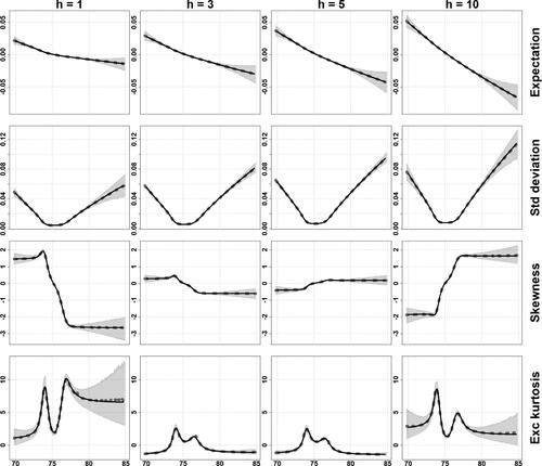
A simulation experiment was conducted to illustrate the results of Proposition 3.1 in the case of a MARMA process. The theoretical conditional moments are compared to model-free non-parametrically estimated counterparts in order to assess the validity of the analytical formulas. Let us consider, for expository purposes, that the price series $(X_t)$ of an asset is modeled by the MARMA process defined as the strictly stationary solution of $(1-0.9F)(1+0.3B)X_t=(1+0.4F)(1-0.3B){\epsilon }_t$, ${\epsilon }_t\stackrel{\text{iid}}{\sim }\mathcal{S}(1.8,0.5,0.2,10)$. We will focus on the conditional moments of the returns at horizon h of $(X_t)$, denoted $R_{t+h}=\frac{X_{t+h}-X_t}{X_t}$. On the one hand, we use the formulas of Proposition 3.1 to compute the theoretical expectation, standard deviation, skewness and excess kurtosis of the returns, conditional on the level X_t = x:(3.8) $$\begin{array}{c}\mu (x,h):=\mathbb{E}\left[R_{t+h}\right|X_t=x],\\ {\sigma }^2(x,h):=\mathbb{E}\left[{(R_{t+h}-\mu (x,h))}^2\right|X_t=x],\\ {\gamma }_1(x,h):=\mathbb{E}\left[{(\frac{R_{t+h}-\mu (x,h)}{\sigma (x,h)})}^3\right|X_t=x],\\ {\gamma }_2(x,h):=\mathbb{E}\left[{(\frac{R_{t+h}-\mu (x,h)}{\sigma (x,h)})}^4\right|X_t=x]-3.\end{array}$$(3.8)

It is just a matter of expanding the powers in the definitions above to express the conditional moments of $R_{t+h}$ in terms of $\mathbb{E}[X_{t+h}^p|X_t],p\in \{1,2,3,4\}$, where $X_t=\sum _{k\in \mathbb{Z}}{a}_k{\epsilon }_{t+k}$ admits an α-stable MA($\infty$) representation whose coefficients are given by Equation (3.7)(3.7) $$\forall k\in \mathbb{Z},\mathrm{}\mathrm{}\hspace{1em}{a}_k=\sum _{\mathcal{l}=-s}^r{\vartheta }_{\mathcal{l}}\mathrm{}\left[\mathrm{}\sum _{i=0}^{q-1}{b}_{1,i} c_{1,k+p+i-\mathcal{l}}+\mathrm{}\sum _{j=0}^{p-1}{b}_{2,j}{c}_{2,k+j-\mathcal{l}}\mathrm{}\right]\mathrm{}\mathrm{},$$(3.7) . On the other hand, we simulate M = 2000 trajectories $x_1^{(m)},x_2^{(m)},\dots ,x_N^{(m)},m=1,\dots ,M$, with $N={10}^7$ observations of the aforementioned MARMA process and obtain model-free estimates of the conditional power moments $\mathbb{E}[X_{t+h}^p|X_t=x]$ using Nadaraya–Watson estimator$${\widehat{E}}^{(m)}(X_{t+h}^p|X_t=x):=\frac{\sum _{i=1}^{N-h}{K}_w(x-x_i^{(m)}){(x_{i+h}^{(m)})}^p}{\sum _{j=1}^{N-h}{K}_w(x-x_j^{(m)})},$$where K_w is the Gaussian kernel with bandwidth w. Empirical counterparts ${\widehat{\mu }}^{(m)}(x,h)$, ${\widehat{\sigma }}^{(m)}(x,h),{\widehat{\gamma }}_1^{(m)}(x,h)$, ${\widehat{\gamma }}_2^{(m)}(x,h),m=1,\dots ,M$, of $\mu (x,h)$, $\sigma (x,h),{\gamma }_1(x,h)$, and ${\gamma }_2(x,h)$ are obtained by substituting the nonparametric estimates ${\widehat{E}}^{(m)}(X_{t+h}^p|X_t=x)$ in Equation (3.8)(3.8) $$\begin{array}{c}\mu (x,h):=\mathbb{E}\left[R_{t+h}\right|X_t=x],\\ {\sigma }^2(x,h):=\mathbb{E}\left[{(R_{t+h}-\mu (x,h))}^2\right|X_t=x],\\ {\gamma }_1(x,h):=\mathbb{E}\left[{(\frac{R_{t+h}-\mu (x,h)}{\sigma (x,h)})}^3\right|X_t=x],\\ {\gamma }_2(x,h):=\mathbb{E}\left[{(\frac{R_{t+h}-\mu (x,h)}{\sigma (x,h)})}^4\right|X_t=x]-3.\end{array}$$(3.8) in place of $\mathbb{E}[X_{t+h}^p|X_t=x]$. We considered prediction horizons $h=1,3,5,10$, conditioning values x in the interval (70, 85)—corresponding to the 0.0005 and 0.9995 quantiles of the marginal distribution of X_t : 99.9% of the probability mass of X_t is supported on (70, 85)—and used a bandwidth of w = 0.1. Letting $N{W}^{(m)}$ denote generically any of ${\widehat{\mu }}^{(m)}$, ${\widehat{\sigma }}^{(m)},{\widehat{\gamma }}_1^{(m)},{\gamma }_2^{(m)}$, we compute for each quantity the point-wise average of Nadarya–Watson estimators as $\overline{NW}(x,h):=\frac{1}{M}{\sum }_{m=1}^{M}N{W}^{(m)}(x,h)$ as well as the point-wise 0.05 and 0.95 quantiles across simulations. Figure 2 compares the theoretical conditional moments obtained using Proposition 3.1 and Equation (3.7)(3.7) $$\forall k\in \mathbb{Z},\mathrm{}\mathrm{}\hspace{1em}{a}_k=\sum _{\mathcal{l}=-s}^r{\vartheta }_{\mathcal{l}}\mathrm{}\left[\mathrm{}\sum _{i=0}^{q-1}{b}_{1,i} c_{1,k+p+i-\mathcal{l}}+\mathrm{}\sum _{j=0}^{p-1}{b}_{2,j}{c}_{2,k+j-\mathcal{l}}\mathrm{}\right]\mathrm{}\mathrm{},$$(3.7) with their empirical nonparametric counterparts. We notice that the average $\overline{NW}$ is very closely matching the theoretical moments curves, and that the theoretical moments lie everywhere within the empirical 0.05–0.95 interquantile. This provides evidence for the sanity of Theorem 2.2 and Proposition 3.1. In addition, we notice that the dispersion of the model-free nonparametric estimators is rather important for X_t = x far from central values, despite the length of the simulated trajectories ($N={10}^7$ observations). This suggests that the analytical formulas can hardly be traded for purely data-driven methods when it comes to estimating the dynamics during extreme events, even with massive amounts of data.

Fig. 2 Conditional expectation, standard deviation, skewness and excess kurtosis (in rows) of the returns $R_{t+h}=(X_{t+h}-X_t)/X_t$ at horizons $h=1,3,5,10$ (in columns) of the ARMA process $(1-0.9F)(1+0.3B)X_t=(1+0.4F)(1-0.3B){\epsilon }_t,{\epsilon }_t\stackrel{\text{iid}}{\sim }\mathcal{S}(1.8,0.5,0.2,10)$ for conditioning values $X_t=x\in (70,85)$ (x-axis of each plot, 99.9% of the probability mass of the marginal distribution of X_t is supported on (70,85)). Black solid lines: theoretical moments (3.8) given by Proposition 3.1 and (3.7); Gray dotted lines: average of Nadaraya–Watson estimators (bandwidth = 0.1) across 2000 simulated trajectories of 10⁷ observations each; Grey shaded areas: empirical 0.05–0.95 interquantile interval across simulations.

To compute the conditional moments in practice, one can now overlook the model-free nonparametric approach and resort to a parametric plug-in strategy: for example, estimate the MARMA and stable parameters by maximum likelihood and plug the parameter estimates in the formulas of Proposition 3.1. An additional experiment reported in Section A.2 of the supplementary file illustrates the reliability of the latter parametric plug-in strategy, and its ability to accurately recover the conditional moments curves for practically relevant sample sizes.

Remark 3.3.

The asymptotic properties of the Nadaraya–Watson for strongly mixing sequences with bounded second order marginal moment have been established by Hansen (2008). In our context, where higher-order conditional moments may be bounded in spite of infinite marginal variance, the validity of the Nadarya–Watson estimator is an open issue. The agreement between the theoretical moment curves and the empirical ones obtained with the Nadaraya–Watson estimator also suggests that the latter’s validity may extend. This is left for further research.

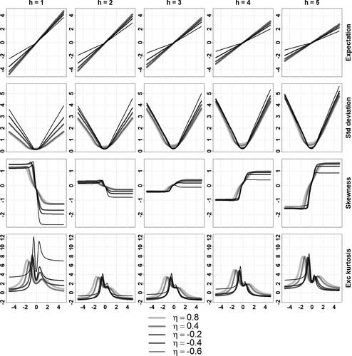
3.3.2 Illustrating the Effects of Parameters on the Conditional Moments

Relying on the analytical formulas of the conditional moments given in Section 2 and Proposition 3.1, we provide some graphical illustration of the conditional moments of α-stable processes. These conditional moments depend on many parameters: the parameters of the errors distributions and the parameters of the time dependence structure, for an arbitrary MA($\infty$), there are infinitely many coefficients involved. To restrict the parameter space, we focus on two types of MARMA processes: MARMA($1,1,1,1$) processes solution of$$(1-\psi F)(1-\varphi B)X_t=(1+\theta F)(1+\eta B){\epsilon }_t,$$and MARMA($2,0,0,1$) processes solution of$$(1-{\psi }_{1}F)(1-{\psi }_{2}F)X_t=(1+\eta B){\epsilon }_t.$$

For the errors, we assume as in the previous sections that ${\epsilon }_t\stackrel{\text{iid}}{\sim }\mathcal{S}(\alpha ,\beta ,\sigma ,\mu )$. These MARMA processes, which are not Markov and for which Proposition 3.1 is, to the best of the author’s knowledge, the only analytical result characterizing their conditional moments, allow to assess the impact of the various AR/MA components on the conditional moments. Figures A1-A6 in the appendix depict these effects on the shape of the conditional expectation, standard deviation, skewness, and excess kurtosis of $X_{t+h}|X_t=x$, at horizons $h=1,2,3,4,5$ and as a function of the conditioning value x for the two types of MARMA processes above.

The revealed patterns feature some characteristic aspects across horizons, processes, and parameters. The conditional expectation curves are either linear or piecewise linear with a non-linearity in the vicinity of central values, while the standard deviation curves are V-shaped, possibly asymmetric. The skewness curves are generally S-shaped, excess kurtosis curves feature two spikes on each flank of the central values, and both the skewness and excess kurtosis flatten out to constant levels for x away from central values. This is expected from Proposition 2.1 for these standardized moments. The general level of the standard deviation curves appears to increase with the forecasting horizon; while the general magnitudes of the skewness and kurtosis curves seem to initially decrease with the horizon before rising again. For large forecasting horizon, we expect the conditional moments of order 2, 3, and 4 to diverge since the marginal moments are infinite.

3.3.3 Cauchy MA($\infty$) Processes

MAR processes with Cauchy errors (stable with α = 1 and β = 0) are a popular benchmark for speculative bubble modeling in the noncausal literature (e.g., Hencic and Gouriéroux 2015; Hecq, Lieb, and Telg 2016; Fries and Zakoian 2019; Gouriéroux, Hencic, and Jasiak 2019; Cavaliere, Nielsen, and Rahbek 2020; Hecq and Voisin 2020). An attractive feature of this class of models is that the Cauchy distribution is one of the special cases in the stable family for which a closed-form density is available. For Cauchy MAR processes with a single noncausal root, that is, as in Equation (3.3)(3.3) $$\psi (F)\varphi (B)X_t=\Theta (F)H(B){\epsilon }_t,$$(3.3) with $\Theta =H=1$, p = 1 and $q\ge 0$, the decomposition into causal and noncausal components (3.6) allows to obtain the conditional moments and density in closed-form. The techniques based on decomposition (3.6) do not extend however, and no result is available for more general (e.g., MARMA, MA($\infty$)) Cauchy noncausal processes.

Let us apply Proposition 3.1 to $X_t=\sum _{k\in \mathbb{Z}}{a}_k{\epsilon }_{t+k}$ with ${\epsilon }_t\stackrel{\text{iid}}{\sim }\mathcal{S}(1,0,\sigma ,0)$ and $(a_k)$ such that Point $\iota )$ guarantees the existence of the first- and second-order moments (e.g., a Cauchy MARMA process). Then, invoking Point $\iota \iota \iota )$ with ${\beta }_1={\lambda }_1={\mu }_1=q_0=0$ since β = 0, we have for any $x\in \mathbb{R}$ and $h\ge 1$,$$\begin{array}{c}\mathbb{E}\left[X_{t+h}\right|X_t=x]={\kappa }_{1}x,\\ \mathbb{V}(X_{t+h}|X_t=x)=({\kappa }_2-{\kappa }_1^2)(x^2+{\sigma }_1^2).\end{array}$$

In particular, if $a_k\ge 0$ for all k, then ${\kappa }_1=\sum _{k\in \mathbb{Z}}\left|a_k\right|(a_{k-h}/a_k)/$ $\sum _{k\in \mathbb{Z}}\left|a_k\right|=1$ and $\mathbb{E}[X_{t+h}|X_t]=X_t$. Proposition 3.1 thus provides a unifying framework for the existing and new results on the conditional moments of stationary MAR and MARMA processes.

Remark 3.4

(Conditional heteroscedasticity of noncausal processes). Gouriéroux and Zakoian (2017) and Fries and Zakoian (2019) highlighted that the Cauchy noncausal AR(1) and MAR($1,q$) processes exhibit GARCH effects in calendar time, although seemingly defined based on iid errors. The above result shows that this property extends to Cauchy MA($\infty$) processes. Figure 2 further illustrates that this is not a specific feature of the Cauchy distribution, and that modeling prices with noncausal α-stable processes also induces conditional heteroscedasticity in the returns for other values of α. In the Cauchy case, the conditional volatility is quadratic in the past values and Fries and Zakoian (2019) underlined that $(X_t)$ admits a semi-strong double autoregressive representation à la Ling (2007). The conditional first and second moments in Proposition 3.1 suggests that a more complex representation may hold in general for $\alpha \ne 1$. Proposition 2.1 ensures nevertheless that the variance of $X_{t+h}|X_t$ is still asymptotically quadratic in the conditioning value. This can be noticed in the example of the following section.

3.3.4 α-Stable Noncausal AR(1)

Let $(X_t)$ be the α-stable noncausal AR(1) solution of $X_t=\rho X_{t+1}+{\epsilon }_t,{\epsilon }_t\stackrel{\text{iid}}{\sim }\mathcal{S}(\alpha ,\beta ,\sigma ,0)$ with $\alpha \in (0,2),\beta \in [-1,1],\sigma >0$ and $0<\left|\rho \right|<1$. Then $\mathbb{E}[|X_{t+h}{|}^{\gamma }|X_t]<+\infty$ for $0\le \gamma <2\alpha +1$ and $h\ge 1$, and the conditional moments, when they exist, are given by Proposition 3.1 with$$\begin{array}{c}{\sigma }_1^{\alpha }=\frac{{\sigma }^{\alpha }}{1-|\rho {|}^{\alpha }},{\beta }_1=\beta \frac{1-|\rho {|}^{\alpha }}{1-{\rho }^{<\alpha >}},\\ {\kappa }_p=|\rho {|}^{\alpha h}{\rho }^{-hp},{\lambda }_p={\beta }_1{({\rho }^{<\alpha >})}^h{\rho }^{-hp},\\ q_0=-\frac{{\beta }_1}{2}\text{ln}\hspace{0.17em}(1+{\rho }^{-2h}),{\mu }_1=\frac{\sigma \beta }{\pi }\frac{{\rho }^h}{1-\rho }\text{ln}\hspace{0.17em}(1+{\rho }^{-2h}),\end{array}$$for $p\in \{1,2,3,4\}$. For $\rho >0$, a clear interpretation of the distribution $X_{t+h}|X_t=x$ appears during bubble episodes, that is, as x becomes large relative to the central values of process $(X_t)$. Letting $\mu (x,h),{\sigma }^2(x,h),{\gamma }_1(x,h)$ and ${\gamma }_2(x,h)$ denote the conditional expectation, variance, skewness and excess kurtosis of $X_{t+h}$ given X_t = x, respectively (as in Equation (3.8)(3.8) $$\begin{array}{c}\mu (x,h):=\mathbb{E}\left[R_{t+h}\right|X_t=x],\\ {\sigma }^2(x,h):=\mathbb{E}\left[{(R_{t+h}-\mu (x,h))}^2\right|X_t=x],\\ {\gamma }_1(x,h):=\mathbb{E}\left[{(\frac{R_{t+h}-\mu (x,h)}{\sigma (x,h)})}^3\right|X_t=x],\\ {\gamma }_2(x,h):=\mathbb{E}\left[{(\frac{R_{t+h}-\mu (x,h)}{\sigma (x,h)})}^4\right|X_t=x]-3.\end{array}$$(3.8) with $R_{t+h}$ replaced by $X_{t+h}$), when they exist, we have$$\begin{array}{c}\mu (x,h)\sim ({\rho }^{-h}x){\rho }^{\alpha h},\\ {\gamma }_1(x,h)\to s\frac{1-2{\rho }^{\alpha h}}{\sqrt{{\rho }^{\alpha h}(1-{\rho }^{\alpha h})}},\\ {\sigma }^2(x,h)\sim {({\rho }^{-h}x)}^2{\rho }^{\alpha h}(1-{\rho }^{\alpha h}),\\ {\gamma }_2(x,h)\to \frac{1}{{\rho }^{\alpha h}}+\frac{1}{1-{\rho }^{\alpha h}}-6,\end{array}$$ as ${\beta }_{1}x\to +\infty$ if $\left|{\beta }_1\right|=1,x\to \pm \infty$ if $\left|{\beta }_1\right|\ne 1$, and s = 1 (s = – 1) if $x\to +\infty$ ($x\to -\infty$). See Section H in the supplementary file for the proof.

The strikingly simplistic forms of the conditional moments of the α-stable noncausal AR(1) during bubble episodes as given above are characteristic of a weighted Bernoulli distribution assigning probability ${\rho }^{\alpha h}$ to the value ${\rho }^{-h}x$ and probability $1-{\rho }^{\alpha h}$ to 0. In the framework of this model, it is thus natural to interpret ${\rho }^{\alpha h}$ as the probability that the bubble survives at least h more time steps, conditionally on having reached the level X_t = x. Such simplification of the dynamics during extreme events is actually not limited to the α-stable noncausal AR(1) and will now be studied in more detail.

4 Forecasting Noncausal Bubble Crashes

For practical econometric purposes, financial bubbles in stock prices, market indexes, and price–dividend ratios are typically characterized as short-lived explosive episodes followed by abrupt or gradual collapses, and are analyzed using reduced form models (Phillips and Shi 2018). An increasing body of literature documents, models and forecasts bubbles in various financial time series using heavy-tailed noncausal processes (Hecq, Lieb, and Telg 2016; Gouriéroux and Zakoian 2017; Fries and Zakoian 2019; Cavaliere, Nielsen, and Rahbek 2020; Giancaterini and Hecq 2020; Hecq and Voisin 2020). In this section, we focus on the dynamics of noncausal processes during such explosive episodes, that is, when the conditioning level of the trajectory takes on large positive or negative values. Specifically, we will focus on the asymptotic behavior of the conditional distribution of ratios of the form $X_{t+h}/X_t$ and $(X_{t+1},\dots ,X_{t+h})/X_t$.

We derive here closed-form expressions of the ex ante crash odds of bubbles generated by noncausal processes. We first formally establish in the case of the noncausal AR(1) that the intuition described above holds. We then show that this intuition non-trivially extends to processes featuring noncausal AR(1)-type bubbles followed by gradual collapses after the peak. We end this section by obtaining an expression of the crash odds in the case of noncausal MA($\infty$) processes.

As we focus on the extreme events, we do not need to fully specify a parametric distribution for the errors $({\epsilon }_t)$ as in Section 3, but only require that their probability tails are similar to those of an α-stable distribution in that they decay as power laws. Formally, we assume that $({\epsilon }_t)$ is an iid error sequence with regularly varying tails:(4.1) $$\mathbb{P}(|{\epsilon }_0|>x)=x^{-\alpha }L(x),\frac{\mathbb{P}({\epsilon }_0>x)}{\mathbb{P}(|{\epsilon }_0|>x)}\underset{x\to +\infty }{\to }\frac{1+\beta }{2}\in [0,1],$$(4.1) with tail parameter $\alpha >0$, asymmetry $\beta \in [-1,1]$ and L any slowly varying function at infinity, that is, such that $L(tx)/L(x)\to 1$ as $x\to +\infty$ for all t > 0. The α-stable distribution, with $\alpha \in (0,2)$ and asymmetry parameter β, is a typical example of distribution whose tails are power law as in Equation (4.1)(4.1) $$\mathbb{P}(|{\epsilon }_0|>x)=x^{-\alpha }L(x),\frac{\mathbb{P}({\epsilon }_0>x)}{\mathbb{P}(|{\epsilon }_0|>x)}\underset{x\to +\infty }{\to }\frac{1+\beta }{2}\in [0,1],$$(4.1) . However, the more general assumption above and the results in the rest of this section encompass not only noncausal processes with α-stable errors, for which we derived the moments in the previous section, but noncausal processes with any power law tailed errors, including (skewed) t-student errors often invoked in the empirical noncausal literature. Note furthermore that the tail exponent α (or degrees of freedom in the case of the t-student) is not restricted to be below 2 in this section but can take any positive value.

4.1 Crash Odds of Noncausal AR(1)-Type Bubbles

4.1.1 Purely Noncausal AR(1): Exponential Bubbles With Instant Collapses

The following proposition provides the conditional distribution of the noncausal AR(1) during explosive bubble episodes.

Proposition 4.1.

Let $(X_t)$ be the noncausal AR(1) process solution of $X_t=\rho X_{t+1}+{\epsilon }_t$ with $0<\rho <1$, iid errors $({\epsilon }_t)$ satisfying (4.1) for some tail exponent $\alpha >0$ and asymmetry $\beta \in [-1,1]$. Then, for any $h\ge 1$, any $\delta \in (0,{\rho }^{-h})$, we have as $x\to +\infty$ $$\begin{array}{c}\mathbb{P}(\frac{X_{t+h}}{X_t}\in [{\rho }^{-h}-\delta ,{\rho }^{-h}+\delta \left]\right|s{X}_t>x)\to {\rho }^{\alpha h},\\ \mathbb{P}(\frac{X_{t+h}}{X_t}\in [-\delta ,\delta \left]\right|s{X}_t>x)\to 1-{\rho }^{\alpha h},\end{array}$$for any $s\in \{-1,+1\}$ if $\beta \in (-1,1)$, and $s=\beta$ if $\left|\beta \right|=1$.

Proof.

See Section I in the supplementary file.

The conditional distribution of the noncausal AR(1) is thus asymptotically degenerate, so that only two values of $X_{t+h}/X_t$, that is, ${\rho }^{-h}$ and 0, have nonzero probabilities. The proposition formalizes the intuition that bubbles generated by a noncausal AR(1) with regularly varying errors feature a geometric survival distribution with probability parameter ${\rho }^{\alpha }$. This interpretation implies that the survival probability does not depend on the current scale of the bubble. Surprisingly, given that the noncausal AR(1) is a Markov process, it further implies that the survival probability of bubbles does not depend at all on the past history: such bubbles display a memory-less property. Several statistics of interest can be easily computed to describe their survival distribution, for example, crash probability at horizon h, hazard rate, expected lifetime. As the bubbles are memory-less, their survival distribution can be fully characterized by the so-called half-life, or median survival time: the duration $h_{1/2}$ such that the crash probability at horizon $h_{1/2}$ is 1/2. More generally, one can be interested in the q-survival quantile, $q\in [0,1]$, that is, the duration h_q such that the survival probability at horizon h_q is equal to $1-q$. Table 1 summarizes the expressions of these descriptive survival statistics for bubbles generated by a noncausal AR(1) model with regularly varying errors. Computing these statistics only requires the knowledge of the AR coefficient ρ and of the tail exponent α. Typically, bubbles with smaller growth rates (ρ closer to unity) and driven by heavier-tailed shocks (smaller α) are likely to last longer.

Table 1 Descriptive survival statistics of bubbles generated by a heavy-tailed noncausal AR(1) with AR coefficient $\rho \in (0,1)$ and tail exponent $\alpha >0$.

Crash probability at hor. h	Hazard rate	Expected life	q-Survival quantile
$1-{\rho }^{\alpha h}$	$1-{\rho }^{\alpha }$	$\frac{1}{1-{\rho }^{\alpha }}$	$\frac{\hspace{0.17em}\text{ln}\hspace{0.17em}(1-q)}{\alpha \hspace{0.17em}\text{ln}\hspace{0.17em}\rho }$

On the one hand, the memory-less property of these bubbles could be appealing from a financial and economic perspective as it implies that the crash date cannot be known with certainty by traders, hence ensuring a form of no-arbitrage condition. Bubbles with crash dates arising according to a constant hazard rate—another feature of the geometric distribution—appear moreover compatible with the implications of game theoretic settings where arbitrageurs attempt to time exponentially increasing bubbles and induce the crash at a random date when the selling pressure they exert is high enough (Matsushima 2013). On the other hand, the memory-less property also implies that no sophisticated method could allow a forecaster to say anything more regarding the future of AR(1) bubbles than “growth or crash” with the probabilities above. In the case of non-exponentially shaped bubbles or if the extreme errors driving bubbles are assumed to be endogenous rather than iid (as in Blasques, Koopman, and Nientker 2018), past history could however play a more central role for prediction.

Remark 4.1

(Parallel with Blanchard and Watson 1982). The dynamics of the noncausal AR(1) during bubble episodes is reminiscent of the classical model proposed by Blanchard and Watson (1982)(4.2) $$X_{t+1}={\rho }^{\ast }{c}_t{X}_t+{ϵ}_t,X_0=0,$$(4.2) where ${\rho }^{\ast }>1,({ϵ}_t)$ is an iid zero-mean and finite variance error sequence, and $(c_t)$ are iid Bernoulli distributed random variables such that $\mathbb{P}(c_t=1)=1-\mathbb{P}(c_t=0)=p\in (0,1)$. This model recurrently generates exponentially shaped explosive bubbles: the trajectory follows an explosive path while c_t = 1 and ends in a crash when c_t = 0. In view of Proposition 4.1, the bubble episodes generated by a noncausal AR(1) with regularly varying errors follow a dynamics à la Blanchard and Watson with ${\rho }^{\ast }={\rho }^{-1}$ and $p={\rho }^{\alpha }$. Interestingly, while Blanchard and Watson’s model is explicitly designed to feature successive bubble/burst cycles, where the burst probability is a free parameter, the noncausal AR(1) generates trajectories where bubble events intersperse calmer periods. The dynamics (4.2) only emerges during bubble events and the crash probability is rather a function of the other model parameters. The structural constraint on the survival probability $p={\rho }^{\alpha }$ has important statistical implications. In the framework of Blanchard and Watson’s model, statistical information about p can only be gathered from the observed durations of past bubbles that have already collapsed. Assuming m bubbles of durations $T_1,\dots ,T_m$ are observed on a given time series, say, generated by (4.2), one could propose $\widehat{p}=m/{\sum }_{i=1}^m{T}_i$ as an estimator for the parameter p of the Bernoulli variables $(c_t)$. In bubble modeling applications, it is however not uncommon to face very small m situations, or even m = 0 in cases where a single explosive and uncollapsed trend is observed. This renders accurate estimation of p difficult at best, and unfeasible at worst. West (1987) even considered p not to be an identifiable parameter. In contrast, the estimation of ${\rho }^{\alpha }$ can exploit more information present in the data: the sample autocorrelations of the time series and the bubble growth rates provide information about ρ, while the tail heaviness of the time series and of the residuals (obtained after estimation of ρ) provide information about α. A maximum likelihood estimation of the noncausal AR(1) assuming a parametric distribution for the errors, such as α-stable or t-student, would suffice to obtain an estimate of ${\rho }^{\alpha }$. Semiparametric approaches could be operative as well, for example, estimating ρ by least squares and α using the Hill estimator.

4.1.2 Mixed Causal–Noncausal AR(1): Exponential Bubbles With Gradual Collapses

To encompass explosive exponential bubble patterns followed by more complex post-peak dynamics, the noncausal literature considered adding a causal component to the noncausal AR(1), resulting in the much-invoked MAR($1,q$) processes (see, for instance, Hecq and Voisin 2020; Gouriéroux, Hencic, and Jasiak 2019). We show here that whatever the form of the causal component adjoined to the noncausal AR(1), that is, whatever the shape of the collapse after the exponential growth episode, the crash probability—or more accurately, the probability of reaching the end of the exponential growth—still follows from a geometric distribution with parameter ${\rho }^{\alpha }$. We do not restrict to the case of MAR processes but actually consider any process $(X_t)$ satisfying Equation (1.1)(1.1) $$X_t=\sum _{k\in \mathbb{Z}}{a}_k{\epsilon }_{t+k},$$(1.1) with $a_k={\rho }^k$ for all $k\ge 0$, and a_k otherwise almost arbitrary for k < 0. Consequently, such a process satisfies the autoregression $X_t=\rho X_{t+1}+Z_t$, where $Z_t:=\sum _{\mathcal{l}\le 0}{b}_{\mathcal{l}}{\epsilon }_{t+\mathcal{l}}$, with $b_{\mathcal{l}}=a_{\mathcal{l}}-\rho a_{\mathcal{l}-1}$ for all $\mathcal{l}\le 0$. Letting $m\ge 1,h\ge 1$, and $\mathit{\rho }:=({\rho }^m,{\rho }^{m-1},\dots ,\rho ,1)$, we will state our result in the context of a forecaster observing an ongoing explosive exponential episode, that is, observing $(X_{t-m},\dots ,X_{t-1},X_t)$ being close to colinear with $\mathit{\rho }$, and wishing to forecast the future path $(X_{t+1},\dots ,X_{t+h})$. The only restriction that we impose on ${(a_k)}_{k\le -1}$ is the one ruling out “collapses” that would be of similar shapes as the initial exponential growth. This assumption is formalized below and the forecasting result follows.

Assumption 1.

There is $ϵ>0$ such that for all $k\le -1$ and $\lambda \in \mathbb{R},\left|\right|\lambda (a_{k+m},\dots ,a_{k+1},a_k)-\mathit{\rho }\left|\right|>ϵ.$

Proposition 4.2.

Let $m\ge 1,h\ge 1,\rho \in (0,1),\alpha >0$ and $(X_t)$ a two-sided MA($\infty$) process with iid errors satisfying (1.1), (3.1)-(3.2) and (4.1) with $a_k={\rho }^k$ for all $k\ge 0$. Denote ${\underset{\_}{\mathit{X}}}_t:=(X_{t-m},\dots ,X_t),{\overline{\mathit{X}}}_{t+h}:=(X_{t+1},\dots ,X_{t+h}),{\mathit{A}}_k:=(a_{k-1},\dots ,a_{k-h})/\left|a_k\right|=({\rho }^{-1},\dots ,{\rho }^{-k},{\rho }^{-k}{a}_{-1},\dots ,{\rho }^{-k}{a}_{k-h})$ for $k\in \{0,\dots ,h\},\left|\right|·\left|\right|$ any norm and $d:=\underset{\stackrel{k,\mathcal{l}\in \{0,\dots ,h\}}{k\ne \mathcal{l}}}{\min }\left|\right|{\mathit{A}}_k-{\mathit{A}}_{\mathcal{l}}\left|\right|$. If Assumption 1 holds for some $ϵ>0$, then we have that d > 0, and for any $\eta \in (0,ϵ),\delta \in (0,d)$,$$\begin{array}{c}\mathbb{P}\left(\right||\frac{{\overline{\mathit{X}}}_{t+h}}{\left|X_t\right|}-s{\mathit{A}}_k||<\delta |\left|X_t\right|>x,\left|\right|\frac{{\underset{\_}{\mathit{X}}}_t}{\left|X_t\right|}-s\mathit{\rho }\left|\right|<\eta )\\ \mathrm{\hspace{1em}}\mathrm{\hspace{1em}}\underset{x\to +\infty }{\to }\{\begin{array}{cc}{\rho }^{\alpha k}(1-{\rho }^{\alpha }),& \mathrm{ }\text{if}\mathrm{ }k\in \{0,\dots ,h-1\},\\ {\rho }^{\alpha h},& \mathrm{ }\text{if}\mathrm{ }k=h.\end{array}\end{array}$$for any $s\in \{-1,+1\}$ if $\beta \in (-1,1)$, and $s=\beta$ if $\left|\beta \right|=1$.

Proof.

See Section J in the supplementary file.

The above result enjoys a very intuitive pattern interpretation. We illustrate this on the example of the MAR(1,1) below. Let us already highlight that the odds of reaching the end of an observed exponential growth episode at some future horizon are of the same form as the crash odds of a purely noncausal AR(1), that is, geometric governed by ${\rho }^{\alpha }$. This drastically simplifies the peak-date prediction exercise for a forecaster, who only has to estimate two parameters and can even afford to stay agnostic as to whatever form the collapse following the peak will take.

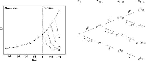
Example 4.1

(Forecasting MAR(1,1) bubbles). Consider the MAR(1,1) process defined as the strictly stationary solution of(4.3) $$(1-\rho F)(1-\varphi B)X_t={\epsilon }_t,$$(4.3) where $\left|\varphi \right|<1$ and $({\epsilon }_t)$ is an iid sequence of regularly varying errors as in (4.1) with tail index $\alpha >0$. The process $(X_t)$ admits the MA($\infty$) representation $X_t=\sum _{k\in \mathbb{Z}}{a}_k{\eta }_{t+k}$, with $a_k={\rho }^k$ for $k\ge 0$; $a_k={\varphi }^{-k}$ for $k\le -1$; and ${\eta }_t:={\epsilon }_t/(1-\rho \varphi )$ for all $t\in \mathbb{Z}$. Note that $({\eta }_t)$ is still an iid regularly varying sequence with index α. Assumption 1 can be shown to hold and Proposition 4.2 applies to $(X_t)$ with the sequence $(a_k)$ as described above and$${\mathit{A}}_k=\{\begin{array}{cc}(\varphi ,{\varphi }^2,\dots ,{\varphi }^h)\hfill & \mathrm{ }\text{for}\mathrm{ }k=0,\hfill \\ (\underset{k}{\underbrace{{\rho }^{-1},{\rho }^{-2},\dots ,{\rho }^{-k}}},\underset{h-k}{\underbrace{{\rho }^{-k}\varphi ,{\rho }^{-k}{\varphi }^2,\dots ,{\rho }^{-k}{\varphi }^{h-k}}})\hfill & \mathrm{ }\text{for}\mathrm{ }k\in \{1,\dots ,h-1\},\hfill \\ ({\rho }^{-1},{\rho }^{-2},\dots ,{\rho }^{-h})\hfill & \mathrm{ }\text{for}\mathrm{ }k=h,\hfill \end{array}$$

If a forecaster observes during an extreme event of process $(X_t)$ that the recent past trajectory has approximately an exponential shape of growth rate ${\rho }^{-1}$, that is, if one observes that $(X_{t-m},\dots ,X_t)$ is approximately colinear to $({\rho }^m,\dots ,\rho ,1)$, then the forecaster may assert that the exponential growth has probability ${\rho }^{\alpha h}$ to continue at least until horizon h, and probability ${\rho }^{\alpha k}(1-{\rho }^{\alpha })$ to stop at an earlier date $k\in \{0,\dots ,h-1\}$. Whenever the exponential growth will reach a peak, the trajectory will then enter a phase of exponential decay, with decay rate $\varphi$. Figure 3 illustrates the forecast interpretation from a trajectorial and probability tree perspectives.

Fig. 3 Illustration of the likely future paths of a bubble generated by a MAR(1,1) process with regularly varying errors as in (4.3). Left panel: trajectorial interpretation with the past observed path in full points, the explosive exponential trend in solid line, and projected likely future paths in dotted lines and circles (graph drawn using $\rho =0.8$ and $\varphi =0.4$. Other positive values of $\varphi$ only change the speed of the decay after the peak. Note however that values $\varphi <0$ are formally allowed by our framework, but would result in differently shaped collapses featuring oscillations). Right panel: probability tree interpretation of the projected future paths with outcomes at the origins and ends of arrows, and probabilities next to the arrows.

Remark 4.2

(Rational bubbles and fat tails). Lux and Sornette (2002) showed that the marginal distribution of rational expectation bubble models à la Blanchard and Watson (1982) necessarily feature regularly varying tails. They further established that a necessary condition for any bubble process $(B_t)$ of the form Equation (4.2)(4.2) $$X_{t+1}={\rho }^{\ast }{c}_t{X}_t+{ϵ}_t,X_0=0,$$(4.2) to abide to the rational expectation condition $B_t=a{\mathbb{E}}_t[B_{t+1}],0<a<1$, is that the tail index of the regular variations be strictly smaller than 1. Invoking evidence gathered by the empirical literature, which does not support such degrees of fat-tailedness, Lux and Sornette conclude that rational bubble models à la Blanchard and Watson are incompatible with the observed statistical properties of financial data.

Interestingly, it appears that MAR processes could reconcile the rational expectations condition with tail indexes greater than 1. In the MAR(1,1) example above, we have that during the inflation phase of a bubble generated by Equation (4.3)(4.3) $$(1-\rho F)(1-\varphi B)X_t={\epsilon }_t,$$(4.3) , the one-step ahead conditional distribution is approximately behaved as$$X_{t+1}=\{\begin{array}{cc}{\rho }^{-1}{X}_t,\hfill & \mathrm{ }\text{with}\mathrm{ }\text{probability}\mathrm{ }{\rho }^{\alpha },\hfill \\ \varphi X_t,\hfill & \mathrm{ }\text{with}\mathrm{ }\text{probability}\mathrm{ }1-{\rho }^{\alpha }.\hfill \end{array}$$

Thus, during the inflation phase of a bubble, ${\mathbb{E}}_t[X_{t+1}]\approx {\rho }^{\alpha }({\rho }^{-1}{X}_t)+(1-{\rho }^{\alpha })\varphi X_t$, and$$X_t\approx {({\rho }^{\alpha -1}+\varphi -{\rho }^{\alpha }\varphi )}^{-1}{\mathbb{E}}_t\left[X_{t+1}\right].$$

The rational expectations condition requires ${({\rho }^{\alpha -1}+\varphi -{\rho }^{\alpha }\varphi )}^{-1}<1$, which can be rewritten as$$\alpha <\hspace{0.17em}\text{ln}\hspace{0.17em}\left(\frac{1-\varphi }{{\rho }^{-1}-\varphi }\right)/\hspace{0.17em}\text{ln}\hspace{0.17em}(\rho ):=f_{\rho }(\varphi ).$$

A straightforward analysis shows that, for any $\rho \in (0,1)$, the function $\varphi \mapsto f_{\rho }(\varphi )$ is strictly increasing on $[0,1)$ and that $f_{\rho }(0)=1,\underset{\varphi \to 1}{\lim }{f}_{\rho }(\varphi )=+\infty$. For $\varphi =0$, one retrieves Lux and Sornette’s result. For $\varphi >0$ however, values of α above 1 are admissible. This suggests that the MAR(1,1), as a process featuring Blanchard/Watson-like bubbles followed by gradual decays, can reconcile the rational expectations condition with regular variation tail indexes above 1. In fact, tail indexes arbitrarily large could be admissible provided the decay after the peak is slow enough ($\varphi$ close enough to 1).

4.2 Crash Odds of Noncausal MA($\infty$) Bubbles

Noncausal MA($\infty$) processes, which encompass in particular higher-order noncausal AR processes and, more generally, arbitrary pre-peak bubble shapes, also feature a simplification of their dynamics during extreme events. The following result generalizes the second convergence in Proposition 4.1 to express the ex ante crash odds of bubbles generated by noncausal MA($\infty$) processes.

Proposition 4.3.

Let $(X_t)$ be a MA($\infty$) process with iid errors as in Equations (1.1)(1.1) $$X_t=\sum _{k\in \mathbb{Z}}{a}_k{\epsilon }_{t+k},$$(1.1) , (3.1)(3.1) $$\sum _{k\in \mathbb{Z}}|a_k{|}^s<+\infty ,\mathrm{ }\text{for}\mathrm{ }\text{some}\mathrm{ }s\in (0,\alpha )\cap [0,1],$$(3.1) , (3.2)(3.2) $$\mathrm{ }\text{and}\mathrm{ }\text{in}\mathrm{ }\text{addition}\mathrm{ }\text{for}\mathrm{ }\alpha =1,\beta \ne 0,\sum _{k\in \mathbb{Z}}\left|a_k\right||\mathrm{}\hspace{0.17em}\text{ln}\hspace{0.17em}|a_k\left|\right|<+\infty .$$(3.2) , and (4.1), with a_k = 0 for all k < 0 and $a_k>0$ for all $k\ge 0$, tail exponent $\alpha >0$ and asymmetry $\beta \in [-1,1]$. Assume also that there is some $ϵ>0$ such $a_k/a_{k+1}>ϵ$ for all $k\ge 0$. Then, for any $h\ge 1$, $\delta \in (0,{ϵ}^h)$,(4.4) $$\mathbb{P}(\frac{X_{t+h}}{X_t}\in [-\delta ,\delta \left]\right|s{X}_t>x)\underset{x\to +\infty }{\to }\sum _{\mathcal{l}=0}^{h-1}{a}_{\mathcal{l}}^{\alpha }/\sum _{k=0}^{+\infty }{a}_k^{\alpha }:=p_{\infty ,h},$$(4.4) for any $s\in \{-1,+1\}$ if $\beta \in (-1,1)$, and $s=\beta$ if $\left|\beta \right|=1$.

Proof.

See Section K in the supplementary file.

Remark 4.3.

The assumptions on the coefficients of the MA($\infty$) representation, namely that $a_k>0$ and $a_k/a_{k+1}>ϵ$ for $k\ge 0$, allow to rule out processes whose extreme events feature oscillations of comparable or larger magnitudes than the crash of the explosive episode itself—for instance due to complex or negative real roots with large moduli in the case of a noncausal AR polynomial. The asymptotics is different in the case of such processes, which are not generating the sought-after bubble patterns.

Similarly to the interpretation of the noncausal AR(1), one can notice that the crash probability of bubbles does not depend on their current scale. Contrary to the noncausal AR(1) however, the survival probabilities could in general be different if the past history of the bubble was accounted for in the conditioning. To investigate this question, one has to characterize the conditional distribution of $X_{t+h}$ given more past information, for example, $X_t,X_{t-1}$… This problem is out of the scope of the current article and is addressed elsewhere (Fries 2018). To evaluate the asymptotic probability (4.4) in practice, only the knowledge of the coefficients $(a_k)$ and of α is needed, whereas asymmetry, scale or location have no role.

We illustrate through simulations that the probability on the left-hand side of Equation (4.4)(4.4) $$\mathbb{P}(\frac{X_{t+h}}{X_t}\in [-\delta ,\delta \left]\right|s{X}_t>x)\underset{x\to +\infty }{\to }\sum _{\mathcal{l}=0}^{h-1}{a}_{\mathcal{l}}^{\alpha }/\sum _{k=0}^{+\infty }{a}_k^{\alpha }:=p_{\infty ,h},$$(4.4) indeed converges to the right-hand side limit as the conditioning value x grows larger. We simulated M = 2000 trajectories of $N={10}^7$ observations of a noncausal AR(3) process. For each simulated trajectory $x_1^{(m)},\dots ,x_N^{(m)},1\le m\le M$, we computed the following estimator of the probability (4.4):(4.5) $${\widehat{p}}_{q,h}^{(m)}:=\left(\sum _{t=1}^{N-h}\mathrm{ }{1}_{\left\{\right|x_{t+h}^{(m)}/x_t^{(m)}|<\delta \}\cap \{x_t^{(m)}>q\}}\right)/\sum _{t=1}^{N-h}\mathrm{ }{1}_{\{x_t^{(m)}>q\}},$$(4.5) for several horizons h and several quantiles q of the marginal distribution of X_t . We perform this exercise twice, first assuming that the AR(3) process is driven by 1.5-stable errors, and then assuming t-student errors with 1.5 degrees of freedom. As our result holds for any heavy-tailed errors in the sense of Equation (4.1)(4.1) $$\mathbb{P}(|{\epsilon }_0|>x)=x^{-\alpha }L(x),\frac{\mathbb{P}({\epsilon }_0>x)}{\mathbb{P}(|{\epsilon }_0|>x)}\underset{x\to +\infty }{\to }\frac{1+\beta }{2}\in [0,1],$$(4.1) and the tail exponents of the error sequences are equal, the estimated crash probabilities should tend to the same limit as q increases. Table 2 gathers the average $\frac{1}{M}{\sum }_{m=1}^M{\widehat{p}}_{q,h}^{(m)}$ of the empirical probabilities across the M simulations along empirical 95% confidence intervals. One notices that the empirical probabilities indeed come very close to the theoretical ones as q increases, both for α-stable and t-student errors. The dispersion of the nonparametric estimators across simulations again indicates that estimating the crash odds of bubble events by purely data-driven methods might be challenging, even with massive amount of data. The expressions given by Propositions 4.1–4.3 thus offer the attractive alternative of computing plug-in estimators of crash odds after having estimated the model parameters.

Table 2 Comparison of theoretical and empirical crash probabilities at horizons h = 1, 5, 10 of bubbles generated by the noncausal AR(3) $X_t=0.9X_{t+1}+0.04X_{t+2}-0.096X_{t+3}+{\epsilon }_t$ with 1.5-stable errors ${\epsilon }_t\stackrel{\text{iid}}{\sim }\mathcal{S}(1.5,1,0.25,0)$ (${\mathcal{S}}_{1.5}$) and t-student errors with 1.5 degrees of freedom ($t_{1.5}$).

			h = 1		h = 5		h = 10
			Mean	95% CI	Mean	95% CI	Mean	95% CI
${\widehat{p}}_{q,h}$	$q_{0.9}$	$t_{1.5}$	8.37	(8.33, 8.41)	33.1	(33.0, 33.2)	42.5	(42.3, 42.7)
		${\mathcal{S}}_{1.5}$	9.12	(9.08, 9.17)	30.7	(30.6, 30.9)	37.6	(37.4, 37.7)
	$q_{0.99}$	$t_{1.5}$	17.7	(17.5, 17.8)	65.9	(65.4, 66.4)	83.4	(83.0, 83.8)
		${\mathcal{S}}_{1.5}$	18.5	(18.3, 18.7)	69.1	(68.7, 69.6)	87.9	(87.5, 88.3)
	$q_{0.999}$	$t_{1.5}$	20.5	(19.9, 21.1)	75.2	(73.7, 76.8)	94.4	(93.3, 95.3)
		${\mathcal{S}}_{1.5}$	20.5	(19.9, 21.1)	75.6	(74.1, 77.1)	94.9	(93.9, 95.8)
	$q_{0.9999}$	$t_{1.5}$	20.7	(18.9, 22.9)	76.2	(71.6, 80.9)	95.4	(92.3, 98.0)
		${\mathcal{S}}_{1.5}$	20.7	(18.9, 22.9)	76.2	(71.4, 81.1)	95.5	(92.4, 98.1)
$p_{\infty ,h}$	$\infty$		20.7	–	76.2	–	95.5	–

NOTES: The theoretical crash probabilities are computed using (4.4). Empirical average (mean) and 95% confidence intervals (95%-CI) of the estimated probabilities are computed using (4.5) on M = 2000 simulated trajectories of $N={10}^7$ observations, with $\delta =0.2$ and for q = q_a several a-quantiles of the marginal distribution of X_t . The quantiles of the marginal distribution of X_t in the case of t-student errors have been estimated by simulations.

Remark 4.4

(Tail dynamics and GARCH effects). We here propose some intuition highlighting the connection between the tail dynamics derived in the previous propositions and the emerging GARCH effects of noncausal processes. Consider for simplicity a purely noncausal process $X_t=\sum _{k\in \mathbb{Z}}{a}_k{\epsilon }_{t+k}$ with $a_k>0$ for $k\ge 0$ and a_k = 0 for k < 0. The ${\epsilon }_t$’s being heavy-tailed and iid, if $X_t=\sum _{s\in \mathbb{Z}}{a}_{s-t}{\epsilon }_s$ at some date t is observed extreme, this likely results from one given ${\epsilon }_{\tau }$ being extreme, for some random date τ in the neighborhood of t such that $a_{\tau -t}\ne 0$, that is, $\tau \ge t$. Because of the independence of the errors, it is likely that the extreme error ${\epsilon }_{\tau }$ is isolated and outweights the other neighboring ${\epsilon }_s$’s contributing to X_t in the sense that ${\epsilon }_s/{\epsilon }_{\tau }\approx 0$ for all $s\ne \tau$ such that $a_{s-t}\ne 0$, that is, $s\ge t$. Thus, we have the approximation$$\begin{array}{c}\frac{X_{t+1}}{X_t}=\frac{a_{\tau -t-1}{\epsilon }_{\tau }+\sum _{s\ne \tau }{a}_{s-t-1}{\epsilon }_s}{a_{\tau -t}{\epsilon }_{\tau }+\sum _{s\ne \tau }{a}_{s-t}{\epsilon }_s}\\ =\frac{a_{\tau -t-1}+\sum _{s\ne \tau }{a}_{s-t-1}{\epsilon }_s/{\epsilon }_{\tau }}{a_{\tau -t}+\sum _{s\ne \tau }{a}_{s-t}{\epsilon }_s/{\epsilon }_{\tau }}\approx \frac{a_{\tau -t-1}}{a_{\tau -t}}.\end{array}$$

In the case of the noncausal AR(1), $a_k={\rho }^k{1}_{k\ge 0}$, and $a_{\tau -t-1}/a_{\tau -t}={\rho }^{-1}\mathrm{ }{1}_{\tau \ge t+1}$ (recall that the random date τ satisfies $1_{\tau \ge t}=1$), which recovers the result of Proposition 4.1: the conditional distribution of $X_{t+1}/X_t$ during extreme events concentrates on the points 0 (crash) and ${\rho }^{-1}$ (growth), and the random date τ has to be interpreted as the peak date of the bubble. Given the information at t, which is assumed to contain at least the value of X_t , the conditional variance of $X_{t+1}$ can now be approximated as$$\mathbb{V}(X_{t+1}|I_t)\approx \mathbb{V}(\frac{a_{\tau -t-1}}{a_{\tau -t}}{X}_t\left|I_t\right)=X_t^2\mathbb{V}\left(\frac{a_{\tau -t-1}}{a_{\tau -t}}\right|I_t).$$

This analysis shows that provided the distribution of τ given I_t is not degenerate, then $\mathbb{V}\left(\frac{a_{\tau -t-1}}{a_{\tau -t}}\right|I_t)>0$ and $(X_t)$ features GARCH effects during extreme events (note that the existence of a nonzero constant such that $a_{k-1}/a_k=\text{const}$ for all $k\ge 0$ is ruled out). Continuing with the example of the noncausal AR(1), the above writes (we recognize the asymptotic variance in Section 3.3.4)$$\begin{array}{c}\mathbb{V}(X_{t+1}|I_t)=X_t^2\mathbb{V}({\rho }^{-1}{1}_{\tau \ge t+1}|I_t)\\ ={({\rho }^{-1}{X}_t)}^2\mathbb{P}(\tau \ge t+1|I_t)\mathbb{P}(\tau <t+1|I_t),\end{array}$$highlighting that the conditional variance of $X_{t+1}$ stems from the uncertainty in the occurrence date of the peak given the available information. Note that this heuristics does not necessarily presume that I_t contains only information about the past values of $(X_t)$. The set I_t could contain information about other variables or noisy proxies of τ (insider information for instance). Section 3.3.4 and Proposition 4.1 lead us to conclude that observing the infinite past of $(X_t)$ (recall that the noncausal AR(1) is Markov) does not induce $\tau |I_t$ to be degenerate and GARCH effects emerge. Only in the case of perfect foresight of τ, that is, $\tau |I_t=\text{const}$, does the GARCH phenomenon seem to vanish.

5 Concluding Remarks

By embedding α-stable two-sided MA($\infty$) processes into the framework of bivariate α-stable random vectors, we described in detail the conditional dependence of $X_{t+h}$ on X_t . We have shown that noncausality plays a crucial role in the existence of conditional moments, and provided expressions for the latter up to the fourth order, when they exist, as well as their asymptotic behaviors when the conditioning variable takes extreme values. We have detailed practical implementation aspects of the conditional moments as well as the contribution of the results to current methodological practices of the empirical noncausal literature. A future empirical investigation could determine whether corresponding patterns in the conditional moments of real data can be identified. These results could serve as a basis to formulate a higher-order moments portfolio allocation problem (e.g., following Jondeau and Rockinger (2006, 2012) where bubble-timing investors optimize over quantities of speculative and safer assets as well as over the holding time through a bubble. Some limitations of the provided conditional moments formulas could be addressed in further research. This includes expanding the conditioning to a set of past values or the entire past, as opposed to conditioning only by the present level of the trajectory. Also, even though Lemma 3.1 allows to extend the formulas of Proposition 3.1 to the conditional moments of, say, $X_{2,t+h}$ given the present level of another process $X_{1,t}$, obtaining a characterization of the moments in the general multivariate case remains an open issue. Furthermore, despite noncausal processes admitting more conditional moments, higher-order conditional moments may nevertheless not exist for smaller values of α -for instance, the conditional skewness and kurtosis when α = 1. Alternative dependence measures capturing, say, conditional asymmetry and heavy-tailedness in such cases could be investigated.

Focusing on explosive bubble episodes generated by heavy-tailed noncausal MA($\infty$) processes, we provided closed-form asymptotic formulas for the predictive distribution, which enjoy very intuitive patterns and probability tree interpretations. This surprisingly revealed that the noncausal AR(1) bubbles are memory-less with a dynamics à la Blanchard and Watson (1982). The survival distribution of such bubbles is geometric and is fully characterized by the AR coefficient ρ and the tail exponent α, both of which can be estimated by classical methods from the data. Even more surprising is the fact that the augmentation of a noncausal AR(1) bubble by an arbitrarily shaped collapse after the peak does not alter the survival distribution of the exponential growth phase of the bubble. From the point of view of a forecaster observing that the past trajectory is approximately exponentially shaped, the likelihood of the peak being reached at some future horizon has the same simple expression in terms of ρ and α whatever is bound to happen after the peak. Of course, the speed of the collapse still impacts how much is at risk in case of downturn. Interestingly, bubbles generated by mixed causal-noncausal processes, and those of a MAR(1,1) in particular, feature an extended Blanchard and Watson dynamics with gradual collapse which appears to reconcile rational expectation bubble models with tail exponents greater than 1, a well-documented statistical property of financial time series (Lux and Sornette 2002). Statistical methods for agnostically estimating the coefficients $(a_k)$ of the MA representation, for example, under low dimensional restrictions, and for robustly estimating the tail index α in locally explosive events could enable more refined evaluation of the crash odds.

Last, the results on bubble crash prediction also raise policy issues. In case a central bank detects the presence of a bubble component in asset prices, estimates its crash probability term structure and concludes that it poses an important threat to macroeconomic stability, it could take the decision to “lean against the wind” (Cecchetti, Genberg, and Wadhwani 2002), that is, to raise interest rates in order to deflate the bubble and bring prices back to warranted levels. To be able to quantify ex ante the influence of such interventions, in view of taking an optimal decision, it would be interesting to extend the nonlinear impulse functions framework proposed by Gouriéroux and Zakoian (2017) (see Section 11 in their online supplementary File) to derive impulse function for the crash probability during bubble events.

Acknowledgments

The author is thankful to the editor, the associate editor and two referees, whose comments have greatly improved the article. The author is extraordinarily indebted to Jean-Michel Zakoïan, and further thanks Denisa-Georgiana Banulescu, Jean-Marc Bardet, Frédérique Bec, Francisco Blasques, Ophélie Couperier, Gilles De Truchis, Elena Dumitrescu, Christian Francq, Christian Gouriéroux, Alain Hecq, Siem Jan Koopman, Jérémy Leymarie, Yang Lu, Andre Lucas, Anders Rahbek, Li Sun, Sean Telg, Arthur Thomas and Elisa Voisin for insightful discussions.

Supplementary Materials

The supplementary materials contains all mathematical proofs, additional examples and simulation experiments referenced in the article, and codes for replicating the main figures and tables.

Additional information

Funding

The author gratefully acknowledges the support of the Groupe des Écoles Nationales d’Économie et Statistique (GENES), the Agence Nationale de la Recherche (via the Project MultiRisk ANR CE26 2016 - CR), and the support of the European Commission (via the Project NONCAUSALBubble H2020-MSCA-IF-2019 896504).

Appendix.

Illustration of the Conditional Moments in Section 3.3.2

Fig. A1 Conditional moments of a stable MARMA(1,1,1,1) for different values of $\mathit{\alpha }$.

Conditional expectation, standard deviation, skewness and excess kurtosis (in rows) of $X_{t+h}$ given X_t = x, for horizons $h=1,2,3,4,5$ (in columns) and conditioning values $X_t=x\in (-5,5)$ (x-axis of each plot), computed using the formulas of Proposition 3.1, where $(X_t)$ is the strictly stationary solution of $(1-0.8F)(1+0.3B)X_t=(1+0.4F)(1-0.3B){\epsilon }_t$, ${\epsilon }_t\stackrel{\text{iid}}{\sim }\mathcal{S}(\alpha ,0.5,0.1,0)$, $\alpha \in \{1.99,1.9,1.8,1.7,1.6\}$.

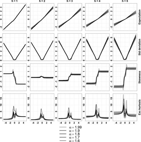
Fig. A2 Conditional moments of a stable MARMA(1,1,1,1) for different values of $\mathit{\beta }$.

Conditional expectation, standard deviation, skewness and excess kurtosis (in rows) of $X_{t+h}$ given X_t = x, for horizons $h=1,2,3,4,5$ (in columns) and conditioning values $X_t=x\in (-5,5)$ (x-axis of each plot), computed using the formulas of Proposition 3.1, where $(X_t)$ is the strictly stationary solution of $(1-0.8F)(1+0.3B)X_t=(1+0.4F)(1-0.3B){\epsilon }_t$, ${\epsilon }_t\stackrel{\text{iid}}{\sim }\mathcal{S}(1.7,\beta ,0.1,0)$, $\beta \in \{0.8,0.4,0,-0.2,-0.6\}$.

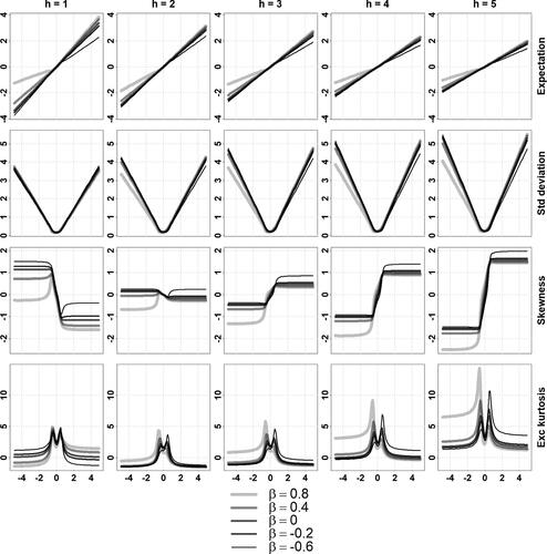
Fig. A3 Conditional moments of a stable MARMA(1,1,1,1) for different values of $\mathit{\psi }$.

Conditional expectation, standard deviation, skewness and excess kurtosis (in rows) of $X_{t+h}$ given X_t = x, for horizons $h=1,2,3,4,5$ (in columns) and conditioning values $X_t=x\in (-5,5)$ (x-axis of each plot), computed using the formulas of Proposition 3.1, where $(X_t)$ is the strictly stationary solution of $(1-\psi F)(1+0.3B)X_t=(1+0.4F)(1-0.3B){\epsilon }_t$, ${\epsilon }_t\stackrel{\text{iid}}{\sim }\mathcal{S}(1.7,0.5,0.1,0)$, $\psi \in \{0.95,0.9,0.85,0.8,0.75\}$.

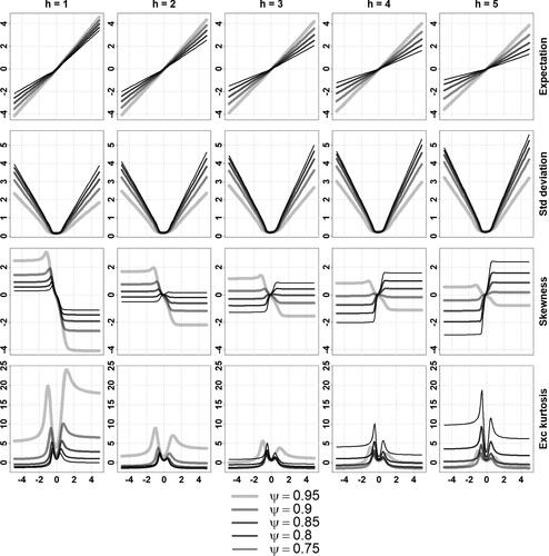
Fig. A4 Conditional moments of a stable MARMA(1,1,1,1) for different values of $\mathit{\varphi }$.

Conditional expectation, standard deviation, skewness and excess kurtosis (in rows) of $X_{t+h}$ given X_t = x, for horizons $h=1,2,3,4,5$ (in columns) and conditioning values $X_t=x\in (-5,5)$ (x-axis of each plot), computed using the formulas of Proposition 3.1, where $(X_t)$ is the strictly stationary solution of $(1-0.8F)(1-\varphi B)X_t=(1+0.4F)(1-0.3B){\epsilon }_t,{\epsilon }_t\stackrel{\text{iid}}{\sim }\mathcal{S}(1.7,0.5,0.1,0)$, $\varphi \in \{0.7,0.4,0,-0.4,-0.7\}$.

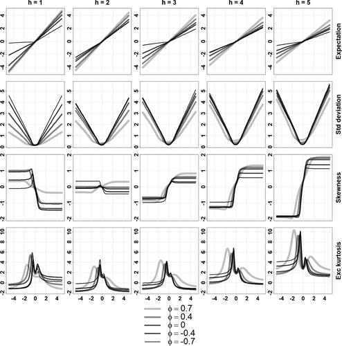
Fig. A5 Conditional moments of a stable MAR(2,0,0,1) for different values of ψ₂.

Conditional expectation, standard deviation, skewness and excess kurtosis (in rows) of $X_{t+h}$ given X_t = x, for horizons $h=1,2,3,4,5$ (in columns) and conditioning values $X_t=x\in (-5,5)$ (x-axis of each plot), computed using the formulas of Proposition 3.1, where $(X_t)$ is the strictly stationary solution of $(1-{\psi }_{1}F)(1-{\psi }_{2}F)X_t=(1+0.9B){\epsilon }_t,{\epsilon }_t\stackrel{\text{iid}}{\sim }\mathcal{S}(1.7,0.5,0.1,0),{\psi }_1=0.8$, ${\psi }_2\in \{0.6,0.3,0,-0.3,-0.6\}$.

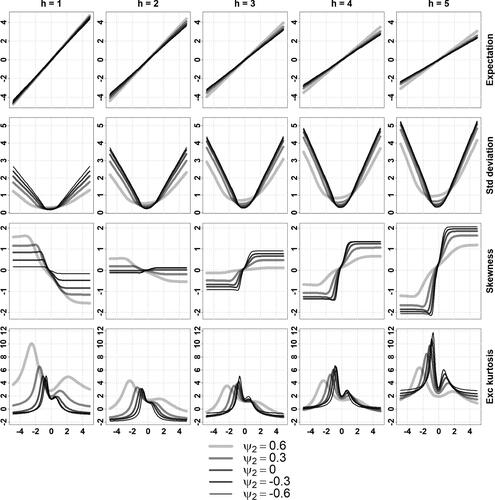
Fig. A6 Conditional moments of a stable MAR(2,0,0,1) for different values of $\mathit{\eta }$.

Conditional expectation, standard deviation, skewness and excess kurtosis (in rows) of $X_{t+h}$ given X_t = x, for horizons $h=1,2,3,4,5$ (in columns) and conditioning values $X_t=x\in (-5,5)$ (x-axis of each plot), computed using the formulas of Proposition 3.1, where $(X_t)$ is the strictly stationary solution of $(1-0.4F)(1-0.8F)X_t=(1+\eta B){\epsilon }_t,{\epsilon }_t\stackrel{\text{iid}}{\sim }\mathcal{S}(1.7,0.5,0.1,0)$, $\eta \in \{0.8,0.4,-0.2,-0.4,-0.6\}$.

References

- Bec, F., Nielsen, H. B., and Saïdi, S. (2020), “Mixed Causal-Noncausal Autoregressions: Bimodality Issues in Estimation and Unit Root Testing,” Oxford Bulletin of Economics and Statistics, 82, 1413–1428. DOI: 10.1111/obes.12372.
- Blanchard, O., and Watson, M. (1982), “Bubbles, Rational Expectations, and Financial Markets,” National Bureau of Economic Research, No. 0945.
- Blasques, F., Koopman, S. J., and Nientker, M. (2018), “A Time-Varying Parameter Model for Local Explosions,” Tinbergen Institute Discussion Paper, No. TI 2018-088/III.
- Cambanis, S., and Miller, G. (1981), “Linear Problems in pth Order and Stable Processes,” SIAM Journal on Applied Mathematics, 41, 43–69. DOI: 10.1137/0141005.
- Cavaliere, G., Nielsen, H. B., and Rahbek, A. (2020), “Bootstrapping Non-Causal Autoregressions: With Applications to Explosive Bubble Modelling,” Journal of Business and Economic Statistics, 38, 55–67. DOI: 10.1080/07350015.2018.1448830.
- Cecchetti, S.G., Genberg, H., and Wadhwani, S. (2002), “Asset Prices in a Flexible Inflation Targeting Framework,” in Asset PriceBubbles: The Implications for Monetary, Regulatory and International Policies, eds. W. C. Hunter, G. G. Kaufman, and M. Pomerleano, Cambridge, MA: MIT Press, 427–4
- Chen, B., Choi, J., and Escanciano, J. C. (2017), “Testing for Fundamental Vector Moving Average Representations,” Quantitative Economics, 8, 149–180. DOI: 10.3982/QE393.
- Cioczek-Georges, R., and Taqqu, M. S. (1995a), “Form of the Conditional Variance for Stable Random Variables,” Statistica Sinica, 351–361.
- Cioczek-Georges, R., and Taqqu, M. S. (1995b), “Necessary Conditions for the Existence of Conditional Moments of Stable Random Variables,” Stochastic Processes and their Applications, 56, 233–246.
- Cioczek-Georges, R., and Taqqu, M. S. (1998), “Sufficient Conditions for the Existence of Conditional Moments of Stable Random Variables,” Stochastic Processes and Related Topics, 35–67.
- Conway, J. B. (1978), Functions of One Complex Variable, New York: Springer-Verlag.
- Diba, B. T., and Grossman, H. I. (1988a), “Explosive Rational Bubbles in Stock Prices?,” The American Economic Review, 78, 520–530.
- Diba, B. T., and Grossman, H. I. (1988b), “The Theory of Rational Bubbles in Stock Prices,” The Economic Journal, 98, 746–754.
- Fries, S. (2018), “Path Prediction of Aggregated α-Stable Moving Averages Using Semi-Norm Representations,” arXiv preprint arXiv:1809.03631.
- Fries, S., and Zakoian, J.-M. (2019), “Mixed Causal-Noncausal AR Processes and the Modelling of Explosive Bubbles,” Econometric Theory, 35, 1234–1270. DOI: 10.1017/S0266466618000452.
- Giancaterini, F., and Hecq, A. (2020), “Inference in Mixed Causal and Noncausal Models With Generalized Student’s t-Distributions,” arXiv: 2012.01888. Maastricht University.
- Gouriéroux, C., Hencic, A., and Jasiak, J. (2019), “Forecast Performance and Bubble Analysis in Noncausal MAR(1,1) Processes,” Toulouse School of Economics.
- Gouriéroux, C., and Jasiak, J. (2016), “Filtering, Prediction and Simulation Methods for Noncausal Processes,” Journal of Time Series Analysis, 37, 405–430. DOI: 10.1111/jtsa.12165.
- Gouriéroux, C., and Jasiak, J. (2018), “Misspecification of Noncausal Order in Autoregressive Processes,” Journal of Econometrics, 205, 226–248.
- Gouriéroux, C., Jasiak, J., and Monfort, A. (2020), “Stationary Bubble Equilibria in Rational Expectation Models,” Journal of Econometrics, 218, 714–735. DOI: 10.1016/j.jeconom.2020.04.035.
- Gouriéroux, C., and Zakoian, J.-M. (2017), “Local Explosion Modelling by Non-Causal Process,” Journal of the Royal Statistical Society, Series B, 79, 737–756. DOI: 10.1111/rssb.12193.
- Hansen, B. E. (2008), “Uniform Convergence Rates for Kernel Estimation With Dependent Data,” Econometric Theory, 24, 726–748. DOI: 10.1017/S0266466608080304.
- Hardin Jr, C. D., Samorodnitsky, G., and Taqqu, M. S. (1991), “Nonlinear Regression of Stable Random Variables,” The Annals of Applied Probability, 582–612. DOI: 10.1214/aoap/1177005840.
- Hecq, A., and Sun, L. (2019), “Identification of Noncausal Models by Quantile Autoregressions,” arXiv: 1904.05952.
- Hecq, A., Lieb, L., and Telg, S. M. (2016), “Identification of Mixed Causal-Noncausal Models in Finite Samples,” Annals of Economics and Statistics, 123/124, 307–331. DOI: 10.15609/annaeconstat2009.123-124.0307.
- Hecq, A., Telg, S., and Lieb, L. (2017a), “Do Seasonal Adjustments Induce Noncausal Dynamics in Inflation Rates?” Econometrics, 5, 48. DOI: 10.3390/econometrics5040048.
- Hecq, A., Telg, S., and Lieb, L. (2017b), “Simulation, Estimation and Selection of Mixed Causal-Noncausal Autoregressive Models: The MARX Package,” Available at SSRN: https://ssrn.com/abstract=3015797.
- Hecq, A., and Voisin, E. (2020), “Forecasting Bubbles With Mixed Causal-Noncausal Autoregressive Models,” Econometrics and Statistics. DOI: 10.1016/j.ecosta.2020.03.007.
- Hencic, A., and Gouriéroux, C. (2015), “Noncausal Autoregressive Model in Application to Bitcoin/USD Exchange Rates,” In Econometrics of Risk, eds. V. N. Huynh, V. Kreinovich, S. Sriboonchitta, and K. Suriya, Cham: Springer International Publishing; pp. 17–40.
- Jondeau, E., and Rockinger, M. (2006), “Optimal Portfolio Allocation Under Higher Moments,” European Financial Management, 12, 29–55. DOI: 10.1111/j.1354-7798.2006.00309.x.
- Jondeau, E., and Rockinger, M. (2012), “On the Importance of Time Variability in Higher Moments for Asset Allocation,” Journal of Financial Econometrics, 10, 84–123.
- Karcher, W., Shmileva, E., and Spodarev, E. (2013), “Extrapolation of Stable Random Fields,” Journal of Multivariate Analysis, 115, 516–536. DOI: 10.1016/j.jmva.2012.11.004.
- Lanne, M., Luoto, J., and Saikkonen, P. (2012), “Optimal Forecasting of Noncausal Autoregressive Time Series,” International Journal of Forecasting, 28, 623–631. DOI: 10.1016/j.ijforecast.2011.08.003.
- Lanne, M., Nyberg, H., and Saarinen, E. (2012), “Does Noncausality Help in Forecasting Economic Time Series?” Economics Bulletin, 32, 2849–2859.
- Lanne, M., and Saikkonen, P. (2011), “Noncausal Autogressions for Economic Time Series,” Journal of Time Series Econometrics, 3, 1–32. DOI: 10.2202/1941-1928.1080.
- Lanne, M., and Saikkonen, P. (2013), “Noncausal Vector Autoregression,” Econometric Theory, 29, 447–481.
- Ling, S. (2007), “A Double AR (p) Model: Structure and Estimation,” Statistica Sinica, 17, 161–175.
- Lux, T., and Sornette, D. (2002), “On Rational Bubbles and Fat Tails,” Journal of Money, Credit and Banking, 34, 589–610. DOI: 10.1353/mcb.2002.0004.
- Matsushima, H. (2003), “Behavioral Aspects of Arbitrageurs in Timing Games Of Bubbles and Crashes,” Journal Of Economic Theory, 148, 858–870. DOI: 10.1016/j.jet.2012.08.002.
- Miller, G. (1978), “Properties of Certain Symmetric Stable Distributions,” Journal of Multivariate Analysis, 8, 346–360. DOI: 10.1016/0047-259X(78)90058-1.
- Phillips, P. C., and Shi, S. P. (2018), “Financial Bubble Implosion and Reverse Regression,” Econometric Theory, 34, 705–753. DOI: 10.1017/S0266466617000202.
- Samorodnitsky, G., and Taqqu, M. S. (1994), Stable Non-Gaussian Random Processes, London: Chapman & Hall, 516–536.
- West, K. D. (1987), “A Specification Test for Speculative Bubbles,” The Quarterly Journal of Economics, 102, 553–580. DOI: 10.2307/1884217.